 Rifai Chai1*
 Sai Ho Ling1
 Phyo Phyo San2
 Ganesh R. Naik1
 Tuan N. Nguyen1
 Yvonne Tran1,3
 Ashley Craig3
 Hung T. Nguyen1
- 1Faculty of Engineering and Information Technology, Centre for Health Technologies, University of Technology, Sydney, NSW, Australia
- 2Data Analytic Department, Institute for Infocomm Research, A*STAR, Singapore, Singapore
- 3Kolling Institute of Medical Research, Sydney Medical School, The University of Sydney, Sydney, NSW, Australia
This paper presents an improvement of classification performance for electroencephalography (EEG)-based driver fatigue classification between fatigue and alert states with the data collected from 43 participants. The system employs autoregressive (AR) modeling as the features extraction algorithm, and sparse-deep belief networks (sparse-DBN) as the classification algorithm. Compared to other classifiers, sparse-DBN is a semi supervised learning method which combines unsupervised learning for modeling features in the pre-training layer and supervised learning for classification in the following layer. The sparsity in sparse-DBN is achieved with a regularization term that penalizes a deviation of the expected activation of hidden units from a fixed low-level prevents the network from overfitting and is able to learn low-level structures as well as high-level structures. For comparison, the artificial neural networks (ANN), Bayesian neural networks (BNN), and original deep belief networks (DBN) classifiers are used. The classification results show that using AR feature extractor and DBN classifiers, the classification performance achieves an improved classification performance with a of sensitivity of 90.8%, a specificity of 90.4%, an accuracy of 90.6%, and an area under the receiver operating curve (AUROC) of 0.94 compared to ANN (sensitivity at 80.8%, specificity at 77.8%, accuracy at 79.3% with AUC-ROC of 0.83) and BNN classifiers (sensitivity at 84.3%, specificity at 83%, accuracy at 83.6% with AUROC of 0.87). Using the sparse-DBN classifier, the classification performance improved further with sensitivity of 93.9%, a specificity of 92.3%, and an accuracy of 93.1% with AUROC of 0.96. Overall, the sparse-DBN classifier improved accuracy by 13.8, 9.5, and 2.5% over ANN, BNN, and DBN classifiers, respectively.
Introduction
Fatigue during driving is a major cause of road accidents in transportation, and therefore poses a significant risk of injury and fatality, not only to the drivers themselves but also to other road users such as passengers, motorbike users, other drivers, and pedestrians (Matthews et al., 2012). Driver fatigue reduces the ability to perform essential driving skills such as vehicle steering control, tracking vehicle speed, visual awareness, and sufficient selective attention during a monotonous driving condition for a long period of time (Lal and Craig, 2001; Wijesuriya et al., 2007; Craig et al., 2012; Jurecki and Stańczyk, 2014). As a result an automated countermeasure for a driver fatigue system with reliable and improved fatigue classification/detection accuracy is needed to overcome the risk of driver fatigue in transportation (Lal et al., 2003; Vanlaar et al., 2008; Touryan et al., 2013, 2014; Chai et al., 2016).
In the digital age, machine learning can be used to provide automated prediction of driver fatigue. Two approaches can be used in machine learning, which are the regression and classification methods. The goal of regression algorithms is the prediction of continuous values to estimate driving performance (Lin et al., 2005; Touryan et al., 2013, 2014). The outcome of classification algorithms is to predict the target class, such as the classification between fatigue and non-fatigue/alert states (Lin et al., 2010; Zhang et al., 2014; Chai et al., 2016; Xiong et al., 2016). The aim of this study is to improve the accuracy of the prediction of fatigue and non-fatigue states. As a result, this study focuses on using an advanced classification method for enhancing the accuracy of a fatigue classification system previously studied (Chai et al., 2016).
As described in a previous paper (Chai et al., 2016), possible driver fatigue assessment includes psychological and physiological measurements (Lal and Craig, 2001; Borghini et al., 2014). For instance, psychological measurement of driver fatigue involves the need for frequent self-report of fatigue status via brief psychometric questionnaires (Lai et al., 2011). Such an approach would be difficult to implement and may well be biased given its subjective nature (Craig et al., 2006). Physiological measurement of the driver fatigue includes video measurement of the face (Lee and Chung, 2012), brain signal measurement using electroencephalography (EEG; Lal et al., 2003; Lin et al., 2005; Craig et al., 2012; Chai et al., 2016), eye movement tracking system using camera and electrooculography (EOG; Hsieh and Tai, 2013), and heart rate measurement using electrocardiography (ECG; Tran et al., 2009; Jung et al., 2014).
Physiological assessment of facial or eye changes using video recording of the driver's face may lead to privacy issues. Physiological measurement strategies like monitoring eye blink rates using EOG and heart rate variability (HRV) using ECG have been shown to reliably detect fatigue (Tran et al., 2009; Hsieh and Tai, 2013). EEG has also been shown to be a reliable method of detecting fatigue, as it directly measures neurophysiological signals that are correlated with mental fatigue (Wijesuriya et al., 2007; Craig et al., 2012; Zhang et al., 2014; Chuang et al., 2015; He et al., 2015; Xiong et al., 2016). Recently, we have shown a classification of EEG-based driver fatigue with the inclusion of new ICA based pre-processing with a promising classification result (Chai et al., 2016), however, it was concluded the classification accuracy needs to be improved. As a result, this paper will extend the work on a potential EEG-based countermeasure driver fatigue system with an improved classification of fatigue vs. alert states.
An EEG-based classification countermeasure system requires several components including EEG signal measurement, signal pre-processing, feature extraction, and classification modules. For feature extraction in EEG analysis, frequency domain data has been widely explored (Lal and Craig, 2001; Craig et al., 2012). Power spectral density (PSD) methods are popular for converting the time domain of EEG signal into the frequency domain (Demandt et al., 2012; Lin et al., 2014). Alternatively, an autoregressive (AR) modeling parametric approach can also be used for feature extraction in an EEG classification system (McFarland and Wolpaw, 2008; Chai et al., 2016; Wang et al., 2016). The advantage of AR modeling is its inherent capacity to model the peak spectra that are characteristic of the EEG signals and it is an all-pole model making it efficient for resolving sharp changes in the spectra. In our previous finding, an AR modeling feature extractor provided superior classification results compared to PSD for EEG-based driver fatigue classification (Chai et al., 2016). Therefore, in this paper, we present the results of applying AR for modeling feature extraction in order to improve the accuracy the classification algorithm. The PSD method is also included for comparison. For the classification, non-linear methods, such as artificial neural networks (ANN), have been used widely in a variety of applications involving EEG (Nguyen, 2008; Casson, 2014). Bayesian neural networks (BNN) have also been used in EEG-based driver fatigue classification (Chai et al., 2016). The Bayesian regularization framework is able to enhance the generalization of neural networks training regardless of finite and/or noisy data.
Recent attention has been focused on improvement of an ANN approach called deep belief networks (DBN; Hinton and Salakhutdinov, 2006; Hinton et al., 2006; Bengio, 2009; LeCun et al., 2015), which involves a fast, unsupervised learning algorithm for the deep generative model, and supervised learning for a discriminative model. The key advantage of this algorithm is the layer-by-layer training for learning a deep hierarchical probabilistic model efficiently as well as a discriminative fine tuning algorithm to optimize performance on the classification problems (Bengio, 2009; LeCun et al., 2015). A DBN classifier is a promising strategy for improving classification of problems including hand-writing character classification (Hinton et al., 2006), speech recognition (Mohamed et al., 2010; Hinton et al., 2012), visual object recognition (Krizhevsky et al., 2012), and other biomedical applications (O'Connor et al., 2013; Stromatias et al., 2015). The training of the DBN is based on the restricted Boltzmann machine (RBM) with layers-wise training of the network per layer at a time from the bottom up (Hinton et al., 2006). Furthermore, the original RBM approach tended to learn a distributed non-sparse representation. A modified version of the RBM using sparse-RBM to form a sparse-deep belief network (sparse-DBN) has shown promising results for modeling low-order features as well as higher-order features for the application of image classification with improved accuracy (Lee et al., 2008; Ji et al., 2014). As a result of this promising advance in classification of complex features, this paper further investigates the classification of EEG signals associated with driver fatigue using the sparse-DBN. For comparison purposes, the results from several different classifiers are included to determine which algorithms are superior with the highest classification performance.
The main contribution of this paper is the combination of the AR modeling feature extractor and sparse-DBN classifier which have not been explored previously for EEG-based driver fatigue classification, with the objective of enhancing the classification performance over past attempts (Chai et al., 2016). The motivation to utilize the sparse-DBN classifier was to investigate its potential superiority for classifying fatigue, in comparison to other classifiers. Sparse-DBN is a semi supervised learning method that combines unsupervised learning for modeling the feature in the pre-training layer and supervised learning for discriminating the feature in the following layer. Incorporating the sparsity in sparse-DBN, achieved with a regularization term that penalizes a deviation of the expected activation of hidden units from a fixed low-level, prevents the network from overfitting, and is able to learn low-level structures as well as high-level structures (Ji et al., 2014).
Background and Methodology
General Structure
The general structure for the EEG-based driver fatigue classification used in this paper is shown in Figure 1 which is divided into four components: (i) the first component involves EEG data collection in a simulated driver fatigue environment; (ii) the second component involves data pre-processing for removing EEG artifact and the moving window segmentation; (iii) the third component involves the features extraction module that converts the signals into useful features; (iv) the fourth component involves the classification module to process the feature and which translates into output via training and classification procedures. The output of the classification comprises two states: fatigue state and alert (non-fatigue) state.
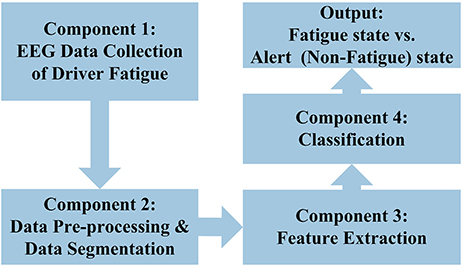
Figure 1. General structure EEG-based driver fatigue classification in this study.
EEG Data Collection
The EEG data collection has been described in a previous paper (Chai et al., 2016). The study was approved by the Human Research Ethics Committee of the University of Technology Sydney (UTS) obtained from previous experiments of driver fatigue study (Craig et al., 2006, 2012; Wijesuriya et al., 2007). The dataset contains electrophysiological data from 43 healthy participants aged between 18 and 55 years who had a current driver's license. The study involved continuous measurement taken during a monotonous simulated driving task followed by post-EEG measures and post-subjective self-report of fatigue. For the simulated driving task, the divided attention steering simulator (DASS) from Stowood scientific instruments was used (Craig et al., 2012). Participants were asked to keep driving at the center of the road in the simulation task. The participants were also required to respond to a target number that appeared in any of the four corners of the computer screen in front of the participants when they were driving in the experiment, so as to record reaction time.
The simulation driving task was terminated if the participant drove off the simulated road for >15 s, or if they showed consistent facial signs of fatigue such as head nodding and extended eyes closure, both determined by analysis of participants' faces that occurred throughout the experiment. Three methods were used to validate fatigue occurrence: (i) using video monitoring for consistent physiological signs of fatigue such as tired eyes, head nodding and extended eye closure, verified further by EOG analysis of blink rate and eye closure; (ii) using performance decrements such as deviation off the road, and (iii) using validated psychometrics such as the Chalder Fatigue Scale and the Stanford Sleepiness Scale. Two participants who did not meet the criterion of becoming fatigued were excluded from the dataset. The validation of fatigue vs. non-fatigue in these participants has been reported in prior studies (Craig et al., 2006, 2012). The EEG signals were recorded using a 32-channel EEG system, the Active-Two system (Biosemi) with electrode positions at: FP1, AF3, F7, F3, FC1, FC5, T7, C3, CP1, CP5, P7, P3, PZ, PO3, O1, OZ, O2, PO4, P4, P8, CP6, CP2, C4, T8, FC6, FC2, F4, F8, AF4, FP2, FZ, and CZ. The recorded EEG data was down sampled from 2,048 to 256 Hz.
Data Pre-processing and Segmentation
For the alert status, the first 5 min of EEG data was selected when the driving simulation task began. For the fatigue status, the data was selected from the last 5 min of EEG data before the task was terminated, after consistent signs of fatigue were identified and verified. Then in each group of data (alert and fatigue), 20 s segments were taken with the segment that was chosen being the first 20 s where EEG signals were preserved. For the sample this was all within the first 1 min of the 5 min selected. Further, artifact removal using an ICA-based method was used to remove blinks, heart, and muscle artifact. As a result, 20 s of the alert state and 20 s of the fatigue state data were available from each participant.
In the pre-processing module before feature extraction, the second-order blind identification (SOBI) and canonical correlation analysis (CCA) were utilized to remove artifacts of the eyes, muscle, and heart signals. The pre-processed data were segmented by applying a moving window of 2 s with overlapping 1.75 s to the 20 s EEG data which provided 73 overlapping segments for each state (fatigue and alert states) as shown in Figure 2. The pre-processing segments were used in the feature extraction module as described in next section.
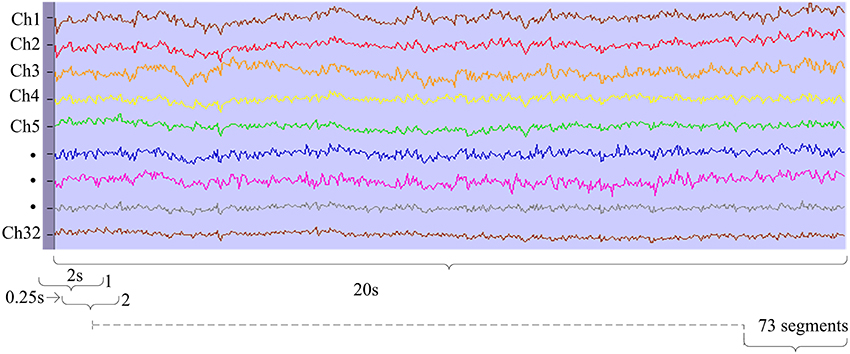
Figure 2. Moving window segmentation for driver fatigue study.
Feature Extraction
For comparison purposes and validity of previous work, a feature extractor using the power spectral density (PSD), a widely used spectral analysis of feature extractor in fatigue studies, is provided in this paper.
An autoregressive (AR) model was also applied as a features extraction algorithm in this study. AR modeling has been used in EEG studies as an alternative to Fourier-based methods, and has been reported to have improved classification accuracy in previous studies compared to spectral analysis of the feature extractor (Brunner et al., 2011; Chai et al., 2016). The advantage of AR modeling is its inherent capacity to model the peak spectra that are characteristic of the EEG signals and it is an all-pole model making it efficient for resolving sharp changes in the spectra. The fast Fourier transform (FFT) is a widely used non-parametric approach that can provide accurate and efficient results, but it does not have acceptable spectral resolution for short data segments (Anderson et al., 2009). AR modeling requires the selection of the model order number. The best AR order number requires consideration of both the signal complexity and the sampling rate. If the AR model order is too low, the whole signal cannot be captured in the model. On the other hand, if the model order is too high, then more noise is captured. In a previous study, the AR order number of five provided the best classification accuracy (Chai et al., 2016). The calculation of the AR modeling was as follows:
where denotes EEG data at time (t), P denotes the AR order number, e(t) denotes the white noise with zero means error and finite variance, and a(k) denotes the AR coefficients.
Classification Algorithm
The key feature of DBN is the greedy layer-by-layer training to learn a deep, hierarchical model (Hinton et al., 2006). The main structure of the DBN learning is the restricted Boltzmann machine (RBM). A RBM is a type of Markov random field (MRF) which is a graphical model that has a two-layer architecture in which the observed data variables as visible neurons are connected to hidden neurons. A RBM is as shown in which m visible neuron [v = (v1, v2, v3,…,vm)] and n hidden neurons [h = (h1, h2,…, hn)] are fully connected via symmetric undirected weights and there is no intra-layer connections within either the visible or the hidden layer.
The connections weights and the biases define a probability over the joint states of visible and hidden neurons through energy function E(v,h), defined as follows:
where wij denotes the weight between vi and hj for all i Î {1,…, m} and j Î {1,…, n}; ai and bj are the bias term associated with the ith and jth visible and hidden neurons; θ = {W,b,a} is the model parameter with symmetric weight parameters Wnm.
For RBM training, the gradient of log probability of a visible vector (v) over the weight wij with the updated rule calculated by constructive divergence (CD) method is as follows:
where η is a learning rate, 〈vihj〉recon is the reconstruction of original visible units which is calculated by setting the visible unit to a random training vector. The updating of the hidden and visible states is considered as follows:
where σ is the logistic sigmoid function.
The original RBM tended to learn a distributed, non-sparse representation of the data, however sparse-RBM is able to play an important role in learning algorithms. In an information-theoretic sense, sparse representations are more efficient than the non-sparse ones, allowing for varying of the effective number of bits per example and able to learn useful low- and high-level feature representations for unlabeled data (i.e., unsupervised learning; Lee et al., 2008; Ji et al., 2014).
This paper uses the sparse-RBM to form the sparse-DBN for EEG-based driver fatigue classification. The sparsity in sparse-DBN is achieved with a regularization term that penalizes a deviation of the expected activation of hidden units from a fixed low-level, which prevents the network from overfitting, as well as allowing it to learn low-level structures as well as high-level structures (Ji et al., 2014). The sparse-RBM is obtained by adding a regularization term to the full data negative log likelihood with the following optimization:
where 𝔼[.] is the conditional expectation given the data, λ is a regularization constant, and p is a constant controlling the sparseness of the hidden neurons hj. The DBN is constructed by stacking a predefined number of RBMs to allow each RBM model in the sequence to receive a different representation of the EEG data. The modeling between visible input (v) and N hidden layer hk is as follows:
where v = h0, P(hk|hk+1) is a conditional distribution for the visible units conditioned on the hidden units of the RBM at level k and P(hl−1,hl) is the visible-hidden joint distribution at the top-level RBM. Two training types of the RBM can be used: generative and discriminative. The generative training of RBM is used as pre-training with un-supervised learning rule. After greedy layer-wise unsupervised learning, the DBN can be used for discriminative ability using the supervised learning. This paper uses a sparse variant of DBN with 2 layers of semi supervised sparse-DBN as shown in Figure 3 with the first layer using the sparse-RBM for generative mode (un-supervised learning) and the second layer using the sparse-RBM in discriminative mode (supervised learning). After layer-by-layer training in DBN, an ANN with back-propagation method is used through the whole classifier to fine-tune the weights for optimal classification.
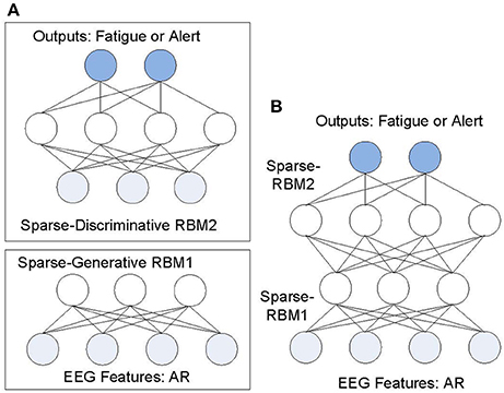
Figure 3. Structure of sparse-DBN for driver fatigue classification: (A) Greedy learning stack of sparse-RBM; (B) the corresponding sparse-DBN.
The performance indicators, including, sensitivity or true positive rate [TPR = TP/(TP+FN)], specificity or true negative rate [TNR = TN/(TN+FP)] and accuracy (TP+TN)/(TP+TN+FP+FN), were used for the performance measurement. TP (true positive) denotes the number of the fatigue data correctly classified as fatigue state. FP (false positive) is the number of alert datasets classified as a fatigue state. TN (true negative) is number of alert datasets correctly classified as an alert state. FN (false negative) is the fatigue datasets classified as an alert state.
For network learning generalization, we presented the results based on two cross-validation techniques: an early stopping technique and k-fold cross-validation. The early stopping technique used the “hold-out cross validation”—one of the widely used cross validations techniques. Basically, it divided the dataset into three subsets (training, validation, and testing sets). The model is trained using the training set while the validation set is periodically used to evaluate the model performance to avoid over-fitting/over-training. The accuracy of the testing set is used as the result of the model's performance. Another cross validation technique is known as k-fold cross-validation (k = 3). In k-fold cross-validation (k = 3), the dataset is divided into three equal (or near equal) sized folds. The training of the network uses 2-folds and the testing the network uses the remaining fold. The process of training and testing is repeated for three possible choices of the subset omitted from the training. The average performance on the three omitted subsets is then used as an estimate of the generalization performance.
Furthermore, a receiver operating characteristic (ROC) graph is used to evaluate further the performance of the proposed method with the compared method for this study. The areas under the curve of the ROC (AUROC) were also computed to evaluate quantitatively the classification performance.
Results
From the 32-EEG channel dataset for the 43 participants (2 participants who did not meet the criterion of becoming fatigued were excluded from original 45 participants), 20 s of alert state and 20 s of fatigue state data were available from each participant. This was fed to the pre-processing module including artifact removal and a 2 s moving window segmentation with overlapping 1.75 s to the 20 s EEG data, providing 73 overlapping segments for each state. As a result, from the 43 participants, a total 6,278 units of datasets were formed for the alert and fatigue states (each state having 3,139 units).
The segmented datasets were fed to the feature extraction module. AR modeling with the order number of 5 was used for the feature extractor as it provided an optimum result from the previous study (Chai et al., 2016). The size of the AR features equaled the AR order number multiplied with 32 units of EEG channels, thus the AR order number of 5 resulted in 160 units of the AR features. For comparison and validity purposes, this paper includes the PSD, a popular feature extractor in the EEG classification for driver fatigue classification. The spectrum of EEG bands consisted of: delta (0.5–3 Hz), theta (3.5–7.5 Hz), alpha (8–13 Hz), and beta activity (13.5–30 Hz). The total power for each EEG activity band was used for the features that were calculated using the numerical integration trapezoidal method, providing 4 units of power values. This resulted in 128 units of total power of PSD for the 32 EEG channels used.
The variant of standard DBN algorithm, sparse-DBN with semi supervised learning used in this paper, comprised of one layer of sparse-RBM with the generative type learning and the second layer of sparse-RBM with discriminative type of learning. The training of the sparse-DBN is done layer-by-layer. The ANN with back-propagation method was used to fine-tune the weights for optimal classification.
For the discriminative learning of sparse-DBN, the total 6,278 datasets were divided into three subsets with similar amounts of number sets: training (2,093 sets) validation (2,093 sets), and testing sets (2,092 sets). The generative learning of sparse-DBN uses unlabeled data from the training sets. For the training of the sparse-DBN using the learning rate (η) of 0.01, the maximum epoch is set to 200, with a regularization constant (λ) of 1, and the constant controlling the sparseness (p) of 0.02. The selection of these training parameters was chosen by trial-and-error, with the chosen values achieving the best training result. Table 1 shows the selection of the regularization constant (λ), with the chosen value of 1 and the constant controlling the sparseness (p) with the chosen value of 0.02, providing lowest the mean square error (MSE) values of 0.00119 (training set) and 0.0521 (validation set) with the iteration number of 69. The average of the MSE values was 0.0046 ± 0.0018 (training set), and 0.0760 ± 0.0124.
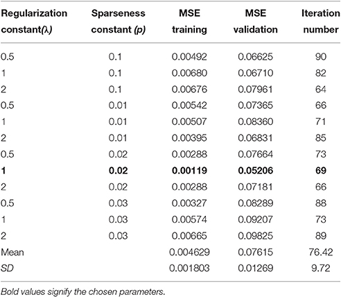
Table 1. Testing several values of regularization constant (λ) and the constant controlling the sparseness (p) in order to select values with the lowest MSE (trial-and-error method).
In order to prevent over-fitting/over-training in the network, a validation-based early stopping method was used for the proposed classifier of sparse-DBN. The plot of the mean square error (MSE) training set and validation set are shown in Figure 4 for classification using AR and sparse-DBN. Table 2 shows the best performance of the training in term of the MSE values and iteration numbers. For comparison, the results for ANN, BNN, and DBN classifier are also included.
Figure 4. Plot of the training and validation MSE for early stopping of classifiers: (A) MSE training and validation of ANN. (B) MSE training of BNN. (C) MSE training of DBN in hidden layer 1 (Generative mode). (D) MSE training of sparse-DBN in hidden layer 1 (Generative mode). (E) MSE training and validation of DBN in hidden layer 2 (Discriminative mode). (F) MSE training and validation of DBN in hidden layer 2 (Discriminative mode).
Table 2. The best MSE and iteration numbers from the training of the classifiers (ANN, BNN, DBN, and Sparse-DBN).
ANN, DBN and sparse-DBN classifiers utilized the early stopping framework (with the dataset divided into training validation and test sets) to prevent the overfitting problem, except for BNN (where the dataset was divided into training and testing). The BNN used a different framework for preventing the overfitting problem utilizing adaptive hyper-parameters in the cost function to prevent the neural network weight from being too large, which would have resulted in poor generalization. As a result, the validation set is not required for the BNN. A detailed analysis of BNN for EEG based driver fatigue classification has been addressed in our previous study (Chai et al., 2016). The core parameters for the training classifiers (ANN, BNN, DBN, and sparse-DBN) are the ANN-based classifier which includes the number of hidden nodes, an activation function, and learning rate. In the BNN classifier, an additional hyper-parameter is introduced to fine tune the optimal structure of the ANN. Further, in the sparse-DBN classifier, the regulation constant and constant controlling of sparseness were introduced for the training the DBN classifier. The DBN and sparse-DBN used two hidden layers: the first hidden layer as generative mode (un-supervised learning) and second hidden layer as discriminative mode (supervised learning).
The mean square error (MSE) of the training set decreased smoothly. Using ANN classifier, the training network stopped after 100 iterations as the MSE validation set reached a maximum fail of 10 times the increment value to ensure no over-training happened with the best validation MSE at 0.115. Using a BNN classifier, the training network stopped after 77 iterations as the conditions are met with the BNN parameters with the best validation MSE at 0.0979. Using a DBN classifier in the first hidden layer (generative mode), the training network stopped after 200 iterations with best MSE at 0.434. Using a DBN classifier in the second hidden layer (discriminative mode), the training network stopped after 68 iterations as the MSE validation set reached maximum fail of 10 times increment value to ensure no over-training happened with the best validation MSE at 0.0649. Using the proposed method of sparse-DBN classifier in the first hidden layer (generative mode), the training network stopped after 200 iterations with the best of MSE at 0.388. Using the proposed method of sparse-DBN classifier in the second hidden layer (discriminative mode), the training network stopped after 69 iterations as the MSE validation set reached maximum fail of 10 times increment value to ensure no over-training happened, with the best validation MSE at 0.0520.
Using the classification results from the validation set, the optimal number of hidden neurons of the sparse-DBN is shown in Figure 5. For the PSD feature extraction, using 10 hidden nodes resulted in the best classification performance. For the AR feature extraction, using 15 hidden nodes produced the best classification performance. These optimal hidden nodes were then used for the training of the network to classify the test set. Also, the results using a different number of layers (2, 3, 5, and 10 layers) are also provided in Figure 5, with the 2 layers (generative mode for the first layer and discriminative mode for second layer) providing the optimal number of layers in this study. This figure shows that using a higher number of layers (3, 5, and 10 layers) results in a lower accuracy compared to results of using only two layers. Therefore, the two layers sparse-DBN was the chosen architecture providing the higher accuracy. The optimal size of sparse-DBN to classify the PSD features of the EEG-based driver fatigue is [128-10-10-2] and the optimal size of sparse DBN to classify the AR feature is [160-15-15-2]. Table 3 shows the results for the classification of the fatigue state vs. alert state using AR feature extractor and sparse-DBN classifier. For a feature extractor comparison and validity of previous result, the result of the classification using PSD feature extractor method is included. Also for classifier comparison, the classification results using original DBN, BNN and ANN are given.
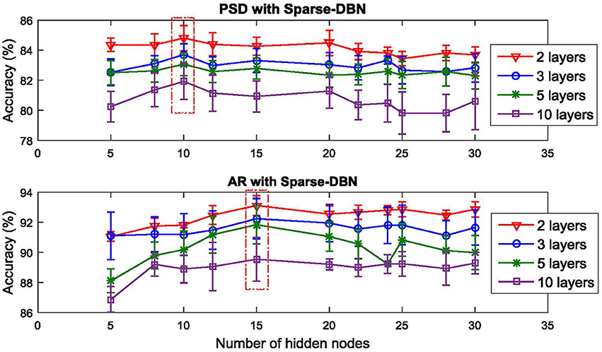
Figure 5. Plot of the optimal number hidden nodes and layers.
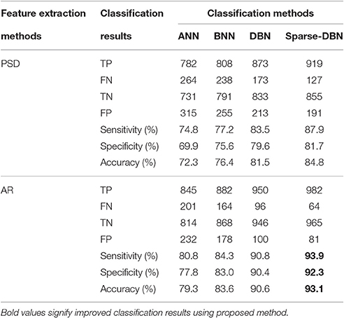
Table 3. Results classification fatigue state vs. alert state for the test set on different feature extractors and classifiers—early stopping approach.
First, for the artificial neural network (ANN) classifier: (i) ANN with PSD, for the fatigue data, of a total with 1,046 units of actual fatigue dataset, 782 units were correctly classified as fatigue states (true positive: TP), resulting in a sensitivity of 74.8%. For the alert group, of a total of 1,046 units of actual alert dataset, 731 units of alert data were correctly classified as alert state (true negative: TN), resulting in a specificity of 69.9%. The combination of ANN and PSD resulted in an accuracy of 72.3%, (ii) ANN with AR, for the fatigue group, of a total of 1,046 units of actual fatigue dataset, 845 units of fatigue data were correctly classified as fatigue states (TP), resulting in a sensitivity of 80.8%. For the alert group, of a total of 1,046 units of actual alert dataset, 814 units of alert data were correctly classified as alert states (TN), resulting in a specificity of 77.8%, while the combination of ANN with AR resulted in an improved accuracy of 79.3% compared to ANN with PSD.
Second, for the Bayesian neural networks (BNN) classifier: (i) BNN with PSD achieved an improvement compared to ANN with PSD, and for the fatigue group, of a total of 1,046 units of actual fatigue dataset, 808 units of fatigue data were correctly classified as fatigue states (TP), resulting in a sensitivity of 77.2%. For the alert state, of a total of 1,046 units of actual alert dataset, 791 units of alert data were correctly classified as alert state (TN), resulting in a specificity of 75.6%. The combination BNN with PSD resulted in an accuracy of 76.4%, (ii) BNN with AR achieved an improvement compared to ANN with AR, and ANN with PSD. BNN with PSD, for the fatigue state, of a total of 1,046 units of actual fatigue data, 882 units were correctly classified as fatigue states (TP), resulting in a sensitivity of 84.3%. For the alert state, of a total of 1,046 units of actual alert data, 868 units of alert data were correctly classified as alert states (TN), resulting in a specificity of 83%. The combination BNN with AR resulted in an accuracy of 83.6%.
Third, when using the deep belief network (DBN) classifier: (i) DBN with PSD achieved a further improvement compared to BNN with PSD, ANN with PSD, and ANN with AR; for the fatigue state, of a total of 1,046 units of actual fatigue data, 873 units of fatigue data were correctly classified as fatigue states (TP), resulting in a sensitivity of 83.5%. For the alert state, of a total of 1,046 units of actual alert data, 833 units of alert data were correctly classified as alert state (TN), resulting in a specificity of 79.6%. The combination DBN with PSD resulted in an accuracy of 81.5%, (ii) DBN with AR achieved further improvement compared to BNN with AR, ANN with AR, DBN with PSD, BNN with PSD, and ANN with PSD, for the fatigue state, of a total of 1,046 units of actual fatigue data, 950 units of fatigue data were correctly classified as fatigue states (TP), resulting in a sensitivity of 90.8%. For the alert state, of a total of 1,046 units of actual alert data, 946 units of alert data were correctly classified as alert states (TN), resulting in a specificity of 90.4%. The combination of DBN with AR resulted in an accuracy of 90.6%.
Fourth, using sparse deep belief networks (sparse-DBN): (i) sparse-DBN with PSD achieved additional improvements compared to DBN with PSD, BNN with PSD, ANN with PSD, BNN with AR, and ANN with AR; for the fatigue state, of a total of 1,046 units of actual fatigue data, 919 units of fatigue data were correctly classified as fatigue states (TP), resulting in a sensitivity of 87.9%. For the alert state, of a total of 1,046 units of actual alert dataset, 855 units of alert data were correctly classified as alert state (TN), resulting in a specificity of 81.7%. The combination sparse-DBN with PSD resulted in an accuracy of 84.8%, (ii) sparse-DBN with AR achieved the most superior result to the other classifier and feature extractor combination with the fatigue state, of a total of 1,046 units of actual fatigue data, 982 units of fatigue data were correctly classified as fatigue states (TP), resulting in a sensitivity of 93.9%. For the alert state, of a total of 1,046 units of actual alert data, 965 units of alert data were correctly classified as alert states (TN), resulting in a specificity of 92.3%. The combination sparse-DBN with AR resulted in best accuracy of 93.1% compared to the other classifier and feature extractor combinations.
Discussion
In summary, using the PSD feature extractor: (i) compared to the ANN classifier, the sparse-DBN classifier improved the classification performance with sensitivity by 13.1% (from 74.8 to 87.9%), specificity by 11.8% (from 69.9 to 81.7%), and accuracy by 12.5% (from 72.3 to 84.8%); (ii) compared to the BNN classifier, the sparse-DBN resulted in improved performance indicators for sensitivity by 10.7% (from 77.2 to 87.9%), specificity by 6.1% (from 75.6 to 81.7%), and accuracy by 8.4% (from 76.4 to 84.8%); (iii) compared to the DBN classifier, the sparse-DBN resulted in improved performance indicators for sensitivity by 4.4% (from 83.5 to 87.9%), specificity by 2.1% (from 79.6 to 81.7%), and accuracy by 3.3% (from 81.5 to 84.8%).
Further, using the AR feature extractor: (i) compared to the ANN classifier, the sparse-DBN classifier improved the classification performance with sensitivity by 13.1% (from 80.8 to 93.9%), specificity by 14.5% (from 77.8 to 92.3%), and accuracy by 13.8% (from 79.3 to 93.1%); (ii) compared to the BNN classifier, the sparse-DBN resulted in improved performance indicators for sensitivity by 9.6% (from 84.3 to 93.9%), specificity by 9.3% (from 83.0 to 92.3%), and accuracy by 9.5% (from 83.6 to 93.1%); (iii) compared to the DBN classifier, the sparse-DBN resulted in improved performance indicators for sensitivity by 3.1% (from 90.8 to 93.9%), specificity by 1.9% (from 90.4 to 92.3%), and accuracy by 2.5% (from 90.6 to 93.1%).
The result of sensitivity (TPR) and specificity (TNR) analyses can also be viewed as the false positive rate (FPR = 1−specificity) and false negative rate (FNR = 1−sensitivity). The FPR is the rate of the non-fatigue (alert) state being incorrectly classified as fatigue state. The FNR is the rate of fatigue state being incorrectly classified as an alert state. As a result, the proposed classifier (sparse-DBN) with the AR feature extractor resulted in a sensitivity (TPR) of 93.9%, FNR of 6.1%, specificity (TNR) of 92.3%, and FPR of 7.7%. For a real-time implementation, an additional debounce algorithm could be implemented. By adding a debounce component, it masks multiple consecutive false positive detection that may decrease the FPR (Bashashati et al., 2006). The real-time implementation with a debounce algorithm will be a future direction in this area of our study.
For the early stopping classifier comparison, a k-fold cross-validation, a popular method for EEG machine learning, is evaluated as well (Billinger et al., 2012). As a result, this study used k-fold cross-validation (k = 3) with the mean value of 10 results of accuracies on each fold. A total of 6,278 datasets were divided into 3-folds (first-fold = 2,093 sets, second-fold = 2,093 sets, and third-fold = 2,092 sets). Overall, the mean value accuracy of 3-folds was reported. Table 4 shows results using k-fold cross validation approach with the chosen AR feature extraction and different classifiers. The result shows that the mean accuracy using the k-fold cross validation approach is comparable to the early stopping approach with the proposed classifier of sparse-DBN as the best classifier (94.8% ± 0.011 of sensitivity, 93.3% ± 0.012 of specificity, and 94.1% ± 0.011 of accuracy) and followed by DBN (90.9% ± 0.005 of sensitivity, 90.5% ± 0.005 of specificity, and 90.7% ± 0.005 of accuracy), BNN (84.8% ± 0.012 of sensitivity, 83.6% ± 0.015 of specificity, and 84.2% ± 0.014 of accuracy), and ANN (81.4% ± 0.010 of sensitivity, 78.4% ± 0.012 of specificity, and 79.9% ± 0.011 of accuracy).
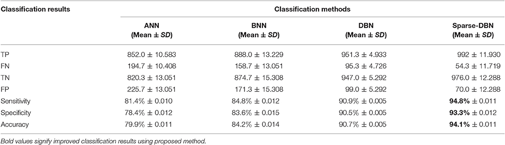
Table 4. Results of classification accuracy fatigue state vs. alert state with chosen AR feature extractors and different classifiers—k-fold cross validation (3-folds) approach.
One-way ANOVA was used to compare the four classifiers (ANN, BNN, DBN, and sparse-DBN) and the resultant p-value was 9.3666e-07. This p-value corresponding to the F-statistic of one-way ANOVA is much lower than 0.05, suggesting that one or more classifiers are significantly different for which Tukey's HSD test (Tukey−Kramer method) was used to detect where the differences were. The critical value of the Tukey−Kramer HSD Q statistic based on the four classifiers and v = 8 degree of freedom for the error term, were significance levels of α = 0.01 and 0.05 (p-value). The critical value for Q, for α of 0.01 (Qα= 0.01) is 6.2044 and the critical value for Q for α of 0.05 (Qα= 0.05) is 4.5293. The Tukey HSD Q-statistic (Qi, j) values were calculated for pairwise comparison of the classifiers. In each pair, the statistical significance is found when Qi, j is more than the critical value of Q. Table 5 presents the Tukey HSD Q-statistic (Qi, j) and Tukey HSD p-value and Tukey HSD inference of the pairwise comparisons. The results in Table 5 show all six pairwise combinations reached statistical significance (*p < 0.05 and **p < 0.01). In addition, to compare the proposed classifier (sparse-DBN) and other classifiers (DBN, BNN, ANN), the sparse-DBN vs. DBN resulted in a p-value of 0.021 (*p < 0.05), while sparse-DBN vs. BNN and sparse-DBN vs. ANN resulted in a p-value of 0.001 (**p < 0.01).
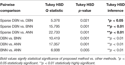
Table 5. Result of Statistical significance of Tukey–Kramer HSD in pairwise comparison.
Overall, the combination of the AR feature extractor and sparse-DBN achieved the best result with improved sensitivity, specificity and accuracy for the classification fatigue vs. alert states in a simulated driving scenario.
Figure 6 shows the results displayed in the receiver operating characteristic (ROC) curve analyses with AR feature extractor and ANN, BNN, DBN, and sparse-DBN classifiers of early stopping (hold-out cross-validation) techniques. The ROC graph is a plot of true positive rate or sensitivity (TPR) on the Y axis and false positive rate (FPR) or 1–specificity on the X-axis by varying different threshold ratios as the sweeping variable. A random performance of a classifier would have a straight line connecting (0, 0) to (1, 1). A ROC curve of the classifier appearing in the lower right triangle suggest it performs worse than random guessing and if the ROC curve appears in the upper left, the classifier is believed to have a superior performance classification (Huang and Ling, 2005; Castanho et al., 2007). All ROC curves in Figure 6 for ANN, BNN, DBN, and sparse-DBN classifier shows the curves plotted in the upper left or above random guess classification. The result also shows that the ROC curve for sparse-DBN classifier achieved the best upper left curve compared to DBN, BNN, and ANN.
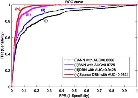
Figure 6. ROC plot with AUC values for AR feature extractor and ANN, BNN, DBN, and sparse-DBN classifiers of early stopping (hold-out cross-validation) technique.
The areas under the curve of ROC (AUROC) were also computed to evaluate quantitatively the classification performance. AUROC represents the probability that the classifier will rank a randomly chosen positive example higher than a randomly chosen negative example, and it exhibits several interesting properties compared to accuracy measurement (Huang and Ling, 2005). The AUROC value lies between 0 and 1 with a higher AUROC value indicating a better classification performance. Figure 6 shows that the classifier using sparse-DBN and AR feature extractor achieved the best performance result with the highest AUROC of 0.9624 compared to original DBN classifier with AUROC of 0.9428, BNN classifier with AUROC 0.8725, and conventional ANN with AUROC of 0.8306.
Figure 7 shows the results displayed in the receiver operating characteristic (ROC) curve analyses with AR feature extractor and ANN, BNN, DBN, and sparse-DBN classifiers of k-fold cross-validation (3-folds) technique with three subplots for each fold. Similar with the ROC plot from the hold-out cross validation technique, all ROC curves in Figure 7 for ANN, BNN, DBN, and sparse-DBN classifier shows the curves plotted in the upper left or above random guess classification, and the ROC curve for the sparse-DBN classifier again had best upper left curve compared to DBN, BNN, and ANN. For the area under the curve analysis, in first-fold (k = 1), sparse-DBN achieved the best AUROC of 0.9643 compared to DBN classifier with AUROC of 0.9484, BNN classifier with AUROC of 0.8879, and ANN classifier with AUROC of 0.8419. For second-fold (k = 2), the sparse-DBN achieved the best AUROC of 0.9673 compared to DBN classifier with AUROC of 0.9520, BNN classifier with AUROC of 0.8968, and ANN classifier with AUROC of 0.8458. For third-fold (k = 3), the sparse-DBN achieved the best AUROC of 0.9627 compared to DBN classifier with AUROC of 0.9434, BNN classifier with AUROC of 0.8858, and ANN classifier with AUROC of 0.8372.
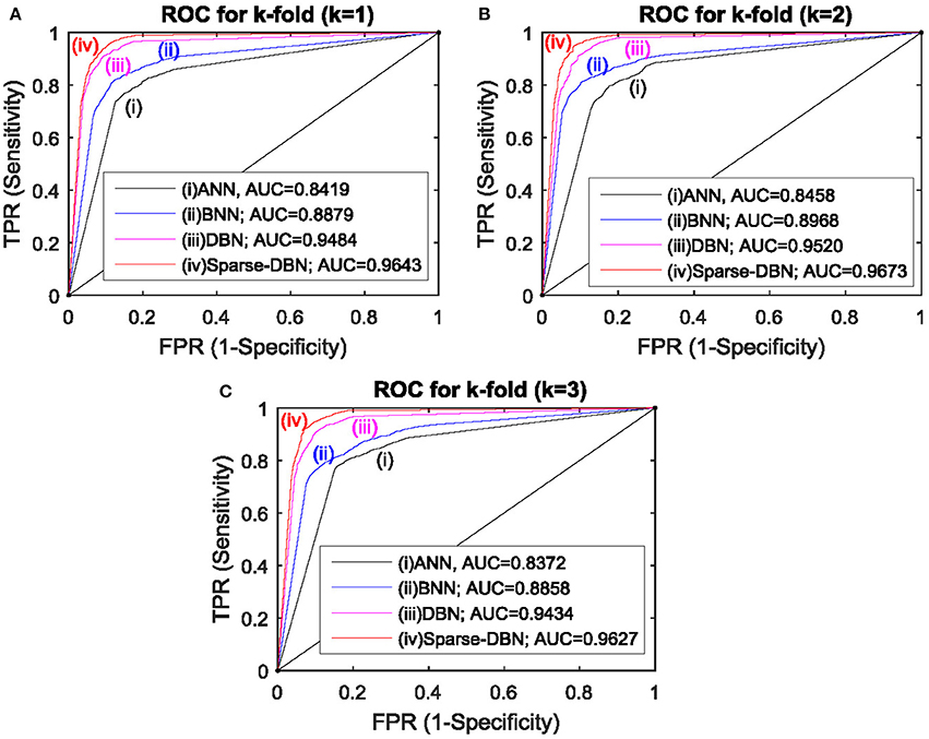
Figure 7. ROC plot with AUC values for AR feature extractor and ANN, BNN, DBN, and sparse-DBN classifiers of k-fold cross validation (k = 3) technique. (A) ROC plot with AUC value for 1st fold. (B) ROC plot with AUC value for 2nd fold. (C) ROC plot with AUC value for 3rd fold.
Our previous work in Chai et al. (2016) showed a promising result with the inclusion of an additional pre-processing component using a recent independent component analysis (ICA) algorithm, AR feature extractor and BNN classifier. However, it was concluded that the performance of the classification needed to be improved. The findings presented in this paper, strongly suggests that the use of an AR feature extractor provides superior results compared to PSD method, and also extends further the study by improving the reliability including the sensitivity, specificity, and accuracy using sparse-DBN classifier in combination with the AR feature extractor, even without the need to include the ICA pre-processing component.
Using chosen classifier parameters, Table 6 shows the comparison of computation times between the proposed classifier (sparse-DBN) and other classifiers (ANN, BNN, and DBN). The computational time is estimated using the MATLAB tic/toc function, where the tic function was called before the program and the toc function afterward on the computer (Intel Core i5−4570 processor 3.20 GHz, 8-GB RAM). The result shows that for the training time, the sparse-DBN required 169.23 ± 0.93 s which was slower compared to other classifiers (86.79 ± 0.24 s for DBN, 55.82 ± 2.77 s for BNN and 24.02 ± 1.04 for ANN). In terms of the testing (classification) time, all classifiers required the same amount of time of 0.03 s or less than a second to complete the task. Although the proposed sparse-DBN required more time to complete the training process, the classifier was able to perform as fast as other classifiers during the testing process. The reason that the testing times of the classifier are comparable to each other was because, after the training process, the final weights were used as constants and in the classification process all classifiers used the same ANN feed-forward classification routine. For the operation of real-time classification, there is no necessity to perform the classifier training again. The classifier just needs to compute the feed forward ANN routine with the saved weight parameters. Thus, sparse-DBN classification time in the runtime mode (execution) is fast, taking less than a second.
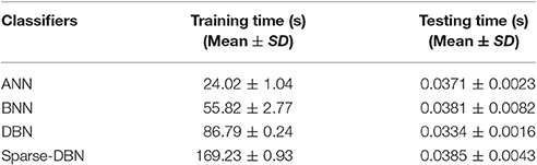
Table 6. Comparison of the training time and testing time for different classifiers.
The potential future direction of this research includes: (i) real-time driver fatigue with the active transfer learning approach for new user adaptation (Wu et al., 2014; Marathe et al., 2016; Wu, 2016), (ii) improvement of the classification result through an intelligent fusion algorithm, and (iii) testing the efficacy of hybrid driver fatigue detection systems using a combination of physiological measurement strategies known to be related to fatigue status, such as brain signal measurement using electroencephalography (EEG), eye movement and facial tracking systems using camera and electrooculography (EOG), and heart rate variability measurement using electrocardiography (ECG).
Conclusions
In this paper, the EEG-based classification of fatigue vs. alert states during a simulated driving task was applied with 43 participants. The AR was used for feature extractor and the sparse-DBN was used as a classifier. For comparison, the PSD feature extractor and ANN, BNN, original DBN were included.
Using the early stopping (hold-out cross validation) evaluation, the results showed that for a PSD feature extractor, the sparse-DBN classifier achieved a superior classification result (sensitivity at 87.9%, specificity at 81.7%, and accuracy at 84.8%) compared to the DBN classifier (sensitivity at 83.5%, specificity at 79.6%, and accuracy at 81.6%), BNN classifier (sensitivity at 77.2%, specificity at 75.6%, and accuracy at 76.4%), and ANN classifier (sensitivity at 74.8%, specificity at 69.9%, and accuracy at 72.3%). Further, using an AR feature extractor and the sparse-DBN achieves a significantly superior classification result (sensitivity at 93.9%, specificity at 92.3%, and accuracy at 93.1% with AUROC at 0.96) compared to DBN classifier (sensitivity at 90.8%, specificity at 90.4%, and accuracy at 90.6% with AUROC at 0.94), BNN classifier (sensitivity at 84.3%, specificity at 83%, and accuracy at 83.6% with AUROC at 0.87) and ANN classifier (sensitivity at 80.8%, specificity at 77.8%, and accuracy at 79.3% with AUROC at 0.83).
Overall the findings strongly suggest that a combination of the AR feature extractor and sparse-DBN provides a superior performance of fatigue classification, especially in terms of overall sensitivity, specificity and accuracy for classifying the fatigue vs. alert states. The k-fold cross-validation (k = 3) also validated that the sparse-DBN with the AR features extractor is the best algorithm compared to the other classifiers (ANN, BNN, and DBN), confirmed by a significance of a p < 0.05.
It is hoped these results provide a foundation for the development of real-time sensitive fatigue countermeasure algorithms that can be applied in on-road settings where fatigue is a major contributor to traffic injury and mortality (Craig et al., 2006; Wijesuriya et al., 2007). The challenge for this type of technology to be implemented will involve valid assessment of EEG and fatigue based on classification strategies discussed in this paper, while using an optimal number of EEG channels (i.e., the minimum number that will result in valid EEG signals from relevant cortical sites) that can be easily applied. These remain the challenges for detecting fatigue using brain signal classification.
Author Contributions
RC performed all data analysis and wrote the manuscript. SL, PS, GN, and TN advised the analysis and edited the manuscript. YT and AC conceptualized the experiment and edited the manuscript. HN supervised the study, advised the analysis, and edited the manuscript.
Funding
This study is funded by “non-invasive prediction of adverse neural events using brain wave activity” from Australian Research Council (DP150102493).
Ethics Statement
Human subjects were given a consent form, which described the experimental procedure and any risks involved (which were minimal). After reading the form, human subjects were asked if they had any questions. Next, human subjects signed the consent form, and then the investigator signed the consent form. The consent forms were stored in a secure filling cabinet in the laboratory.
Conflict of Interest Statement
The authors declare that the research was conducted in the absence of any commercial or financial relationships that could be construed as a potential conflict of interest.
The reviewer SL and handling Editor declared their shared affiliation, and the handling Editor states that the process nevertheless met the standards of a fair and objective review.
Acknowledgments
The authors would like to thank Dr. Nirupama Wijesuriya for her contribution to the work for collecting the data in this study.
References
Anderson, N. R., Wisneski, K., Eisenman, L., Moran, D. W., Leuthardt, E. C., Krusienski, D. J., et al. (2009). An offline evaluation of the autoregressive spectrum for electrocorticography. IEEE Trans. Biomed. Eng. 56, 913–916. doi: 10.1109/TBME.2009.2009767
Bashashati, A., Fatourechi, M., Ward, R. K., and Birch, G. E. (2006). User customization of the feature generator of an asynchronous brain interface. Ann. Biomed. Eng. 34, 1051–1060. doi: 10.1007/s10439-006-9097-5
Bengio, Y. (2009). Learning deep architectures for AI. Found. Trends Mach. Learn. 2, 1–127. doi: 10.1561/2200000006
Billinger, M., Daly, I., Kaiser, V., Jin, J., Allison, B. Z., Müller-Putz, G. R., et al. (2012). “Is it significant? Guidelines for reporting BCI performance,” in Towards Practical Brain-Computer Interfaces, eds B. Z. Allison, S. Dunne, R. Leeb, J. D. R. Millán, and A. Nijholt (Berlin; Heidelberg: Springer Verlag), 333–354.
Borghini, G., Astolfi, L., Vecchiato, G., Mattia, D., and Babiloni, F. (2014). Measuring neurophysiological signals in aircraft pilots and car drivers for the assessment of mental workload, fatigue and drowsiness. Neurosci. Biobehav. Rev. 44, 58–75. doi: 10.1016/j.neubiorev.2012.10.003
Brunner, C., Billinger, M., Vidaurre, C., and Neuper, C. (2011). A comparison of univariate, vector, bilinear autoregressive, and band power features for brain–computer interfaces. Med. Biol. Eng. Comput. 49, 1337–1346. doi: 10.1007/s11517-011-0828-x
Casson, A. J. (2014). Artificial Neural Network classification of operator workload with an assessment of time variation and noise-enhancement to increase performance. Front. Neurosci. 8:372. doi: 10.3389/fnins.2014.00372
Castanho, M. J., Barros, L. C., Yamakami, A., and Vendite, L. L. (2007). Fuzzy receiver operating characteristic curve: an option to evaluate diagnostic tests. IEEE Trans. Inf. Technol. Biomed. 11, 244–250. doi: 10.1109/TITB.2006.879593
Chai, R., Naik, G. R., Nguyen, T. N., Ling, S. H., Tran, Y., Craig, A., et al. (2016). Driver Fatigue Classification with Independent Component by Entropy Rate Bound Minimization Analysis in an EEG-based System. IEEE J. Biomed. Health Informat. PP, 1–1. doi: 10.1109/JBHI.2016.2532354
Chuang, C.-H., Huang, C.-S., Ko, L.-W., and Lin, C.-T. (2015). An EEG-based perceptual function integration network for application to drowsy driving. Knowl. Based Syst. 80, 143–152. doi: 10.1016/j.knosys.2015.01.007
Craig, A., Tran, Y., Wijesuriya, N., and Boord, P. (2006). A controlled investigation into the psychological determinants of fatigue. Biol. Psychol. 72, 78–87. doi: 10.1016/j.biopsycho.2005.07.005
Craig, A., Tran, Y., Wijesuriya, N., and Nguyen, H. (2012). Regional brain wave activity changes associated with fatigue. Psychophysiology 49, 574–582. doi: 10.1111/j.1469-8986.2011.01329.x
Demandt, E., Mehring, C., Vogt, K., Schulze-Bonhage, A., Aertsen, A., and Ball, T. (2012). Reaching movement onset- and end-related characteristics of EEG spectral power modulations. Front. Neurosci. 6:65. doi: 10.3389/fnins.2012.00065
He, Q., Li, W., Fan, X., and Fei, Z. (2015). Driver fatigue evaluation model with integration of multi-indicators based on dynamic Bayesian network. IET Intell. Trans. Syst. 9, 547–554. doi: 10.1049/iet-its.2014.0103
Hinton, G., Deng, L., Yu, D., Dahl, G. E., Mohamed, A. R., Jaitly, N., et al. (2012). Deep neural networks for acoustic modeling in speech recognition: the shared views of four research groups. IEEE Signal Process. Mag. 29, 82–97. doi: 10.1109/MSP.2012.2205597
Hinton, G. E., Osindero, S., and Teh, Y.-W. (2006). A fast learning algorithm for deep belief nets. Neural Comput. 18, 1527–1554. doi: 10.1162/neco.2006.18.7.1527
Hinton, G. E., and Salakhutdinov, R. R. (2006). Reducing the dimensionality of data with neural networks. Science 313, 504–507. doi: 10.1126/science.1127647
Hsieh, C.-S., and Tai, C.-C. (2013). An improved and portable eye-blink duration detection system to warn of driver fatigue. Instrum. Sci. Technol. 41, 429–444. doi: 10.1080/10739149.2013.796560
Huang, J., and Ling, C. X. (2005). Using AUC and accuracy in evaluating learning algorithms. IEEE Trans. Knowl. Data Eng. 17, 299–310. doi: 10.1109/TKDE.2005.50
Ji, N.-N., Zhang, J.-S., and Zhang, C.-X. (2014). A sparse-response deep belief network based on rate distortion theory. Pattern Recognit. 47, 3179–3191. doi: 10.1016/j.patcog.2014.03.025
Jung, S. J., Shin, H. J., and Chung, W. J. (2014). Driver fatigue and drowsiness monitoring system with embedded electrocardiogram sensor on steering wheel. IET Intell. Transp. Syst. 8, 43–50. doi: 10.1049/iet-its.2012.0032
Jurecki, R. S., and Stańczyk, T. L. (2014). Driver reaction time to lateral entering pedestrian in a simulated crash traffic situation. Transp. Res. Part F Traffic Psychol. Behav. 27, 22–36. doi: 10.1016/j.trf.2014.08.006
Krizhevsky, A., Sutskever, I., and Hinton, G. E. (2012). “Imagenet classification with deep convolutional neural networks,” in Advances in Neural Information Processing Systems (Lake Tahoe), 1097–1105.
Lai, J.-S., Cella, D., Choi, S., Junghaenel, D. U., Christodoulou, C., Gershon, R., et al. (2011). How item banks and their application can influence measurement practice in rehabilitation medicine: a PROMIS fatigue item bank example. Arch. Phys. Med. Rehabil. 92, S20–S27. doi: 10.1016/j.apmr.2010.08.033
Lal, S. K., and Craig, A. (2001). A critical review of the psychophysiology of driver fatigue. Biol. Psychol. 55, 173–194. doi: 10.1016/S0301-0511(00)00085-5
Lal, S. K., Craig, A., Boord, P., Kirkup, L., and Nguyen, H. (2003). Development of an algorithm for an EEG-based driver fatigue countermeasure. J. Saf. Res. 34, 321–328. doi: 10.1016/S0022-4375(03)00027-6
LeCun, Y., Bengio, Y., and Hinton, G. (2015). Deep learning. Nature 521, 436–444. doi: 10.1038/nature14539
Lee, B. G., and Chung, W. Y. (2012). Driver alertness monitoring using fusion of facial features and bio-signals. IEEE Sensors J. 12, 2416–2422. doi: 10.1109/JSEN.2012.2190505
Lee, H., Ekanadham, C., and Ng, A. Y. (2008). “Sparse deep belief net model for visual area V2,” in Advances in Neural Information Processing Systems (Vancouver), 873–880.
Lin, C. T., Chang, C. J., Lin, B. S., Hung, S. H., Chao, C. F., and Wang, I. J. (2010). A real-time wireless brain-computer interface system for drowsiness detection. IEEE Trans. Biomed. Circuits Syst. 4, 214–222. doi: 10.1109/TBCAS.2010.2046415
Lin, C. T., Chuang, C. H., Huang, C. S., Tsai, S. F., Lu, S. W., Chen, Y. H., et al. (2014). Wireless and wearable EEG system for evaluating driver vigilance. IEEE Trans. Biomed. Circuits Syst. 8, 165–176. doi: 10.1109/TBCAS.2014.2316224
Lin, C.-T., Wu, R.-C., Jung, T.-P., Liang, S.-F., and Huang, T.-Y. (2005). Estimating driving performance based on EEG spectrum analysis. EURASIP J. Appl. Signal Process. 2005, 3165–3174. doi: 10.1155/ASP.2005.3165
Marathe, A. R., Lawhern, V. J., Wu, D., Slayback, D., and Lance, B. J. (2016). Improved neural signal classification in a rapid serial visual presentation task using active learning. IEEE Trans. Neural Syst. Rehab. Eng. 24, 333–343. doi: 10.1109/TNSRE.2015.2502323
Matthews, G., Desmond, P. A., Neubauer, C., and Hancock, P. A. (2012). The Handbook of Operator Fatigue. Surrey: Ashgate Publishing, Ltd.
McFarland, D. J., and Wolpaw, J. R. (2008). Sensorimotor rhythm-based brain–computer interface (BCI): model order selection for autoregressive spectral analysis. J. Neural Eng. 5, 155. doi: 10.1088/1741-2560/5/2/006
Mohamed, A.-R., Yu, D., and Deng, L. (2010). “Investigation of full-sequence training of deep belief networks for speech recognition,” in INTERSPEECH, 2846–2849.
Nguyen, H. T. (2008). Intelligent technologies for real-time biomedical engineering applications. Int. J. Autom. Control 2, 274–285. doi: 10.1504/IJAAC.2008.022181
O'Connor, P., Neil, D., Liu, S.-C., Delbruck, T., and Pfeiffer, M. (2013). Real-time classification and sensor fusion with a spiking deep belief network. Front. Neurosci. 7:178. doi: 10.3389/fnins.2013.00178
Stromatias, E., Neil, D., Pfeiffer, M., Galluppi, F., Furber, S. B., and Liu, S.-C. (2015). Robustness of spiking Deep Belief Networks to noise and reduced bit precision of neuro-inspired hardware platforms. Front. Neurosci. 9:222. doi: 10.3389/fnins.2015.00222
Touryan, J., Apker, G., Kerick, S., Lance, B., Ries, A. J., and McDowell, K. (2013). “Translation of EEG-based performance prediction models to rapid serial visual presentation tasks,” in International Conference on Augmented Cognition (Las Vegas), 521–530.
Touryan, J., Apker, G., Lance, B. J., Kerick, S. E., Ries, A. J., and McDowell, K. (2014). Estimating endogenous changes in task performance from EEG. Front. Neurosci. 8:155. doi: 10.3389/fnins.2014.00155
Tran, Y., Wijesuriya, N., Tarvainen, M., Karjalainen, P., and Craig, A. (2009). The relationship between spectral changes in heart rate variability and fatigue. J. Psychophysiol. 23, 143–151. doi: 10.1027/0269-8803.23.3.143
Vanlaar, W., Simpson, H., Mayhew, D., and Robertson, R. (2008). Fatigued and drowsy driving: a survey of attitudes, opinions and behaviors. J. Saf. Res. 39, 303–309. doi: 10.1016/j.jsr.2007.12.007
Wang, G., Sun, Z., Tao, R., Li, K., Bao, G., and Yan, X. (2016). Epileptic seizure detection based on partial directed coherence analysis. IEEE J. Biomed. Health Informat. 20, 873–879. doi: 10.1109/JBHI.2015.2424074
Wijesuriya, N., Tran, Y., and Craig, A. (2007). The psychophysiological determinants of fatigue. Int. J. Psychophysiol. 63, 77–86. doi: 10.1016/j.ijpsycho.2006.08.005
Wu, D. (2016). Online and offline domain adaptation for reducing BCI calibration effort. IEEE Trans. Hum. Mach. Syst. PP, 1–14. doi: 10.1109/THMS.2016.2608931
Wu, D., Lance, B., and Lawhern, V. (2014). “Transfer learning and active transfer learning for reducing calibration data in single-trial classification of visually-evoked potentials,” in 2014 IEEE International Conference on Systems, Man, and Cybernetics (San Diego, CA: SMC), 2801–2807. doi: 10.1109/smc.2014.6974353
Xiong, Y., Gao, J., Yang, Y., Yu, X., and Huang, W. (2016). Classifying driving fatigue based on combined entropy measure using EEG signals. Int. J. Control Automat. 9, 329–338. doi: 10.14257/ijca.2016.9.3.30
Keywords: electroencephalography, driver fatigue, autoregressive model, deep belief networks, sparse-deep belief networks
Citation: Chai R, Ling SH, San PP, Naik GR, Nguyen TN, Tran Y, Craig A and Nguyen HT (2017) Improving EEG-Based Driver Fatigue Classification Using Sparse-Deep Belief Networks. Front. Neurosci. 11:103. doi: 10.3389/fnins.2017.00103
Received: 04 October 2016; Accepted: 17 February 2017;
Published: 07 March 2017.
Edited by:
Jianhua Zhang, East China University of Science and Technology, ChinaReviewed by:
Sunan Li, East China University of Science and Technology, ChinaZhong Yin, University of Shanghai for Science and Technology, China
Amar R. Marathe, U.S. Army Research Laboratory, USA
Copyright © 2017 Chai, Ling, San, Naik, Nguyen, Tran, Craig and Nguyen. This is an open-access article distributed under the terms of the Creative Commons Attribution License (CC BY). The use, distribution or reproduction in other forums is permitted, provided the original author(s) or licensor are credited and that the original publication in this journal is cited, in accordance with accepted academic practice. No use, distribution or reproduction is permitted which does not comply with these terms.
*Correspondence: Rifai Chai, cmlmYWkuY2hhaUB1dHMuZWR1LmF1