Motion artifacts removal and evaluation techniques for functional near-infrared spectroscopy signals: A review

With the emergence of an increasing number of functional near-infrared spectroscopy (fNIRS) devices, the significant deterioration in measurement caused by motion artifacts has become an essential research topic for fNIRS applications. However, a high requirement for mathematics and programming limits the number of related researches. Therefore, here we provide the first comprehensive review for motion artifact removal in fNIRS aiming to (i) summarize the latest achievements, (ii) present the significant solutions and evaluation metrics from the perspective of application and reproduction, and (iii) predict future topics in the field. The present review synthesizes information from fifty-one journal articles (screened according to three criteria). Three hardware-based solutions and nine algorithmic solutions are summarized, and their application requirements (compatible signal types, the availability for online applications, and limitations) and extensions are discussed. Five metrics for noise suppression and two metrics for signal distortion were synthesized to evaluate the motion artifact removal methods. Moreover, we highlight three deficiencies in the existing research: (i) The balance between the use of auxiliary hardware and that of an algorithmic solution is not clarified; (ii) few studies mention the filtering delay of the solutions, and (iii) the robustness and stability of the solution under extreme application conditions are not discussed.

Introduction

Functional near-infrared spectroscopy (fNIRS) is a non-invasive brain imaging technique that uses near-infrared light (typically of wavelengths between 650 and 1,000 nm) to monitor hemodynamics changes in the cortical layer. Compared to electroencephalography (EEG), fNIRS enables to measure brain-activity related hemodynamics in terms of cerebral oxygenation and is less susceptible to electric noises (Huppert et al., 2009; Tak and Ye, 2014; Naseer and Hong, 2015; Chiarelli et al., 2017; Afkhami et al., 2019; Ghafoor et al., 2019; Khan et al., 2021). In addition, fNIRS can be integrated into a portable, wearable, and ergonomic device at low costs and operational expenses, making it a superior candidate for a user-friendly brain-computer interface system compared to other modalities, such as functional magnetic resonance imaging (fMRI) and magnetoencephalography (MEG) (Hu et al., 2010; Piper et al., 2014; Scholkmann et al., 2014a; Pinti et al., 2015; Wyser et al., 2017; Zhao and Cooper, 2018; Hong and Zafar, 2018; Zhao H. B. et al., 2020, 2021; Ghafoor et al., 2021; Huang and Hong, 2021).

Fantini et al. (1999) reported that the artifacts caused by subjects’ movements, specifically motion artifacts (MAs), can significantly influence the quality of the recorded optical signals of fNIRS. Some studies claimed that MAs reduce the signal-to-noise ratio (SNR) of fNIRS signals (Izzetoglu et al., 2005; Izzetoglu et al., 2010). Researchers have also verified that using MA removal techniques can ameliorate classification accuracy in cognition experiments (Zhou et al., 2021). Therefore, the issue concerning the causes, characteristics, and rejection methods of MAs in fNIRS signals is a crucial topic in fNIRS studies (Safaie et al., 2013; Piper et al., 2014).

During the early days, researchers skipped the analysis or discarded the data set when the measured signals were significantly corrupted by motion artifacts (Bartocci et al., 2000; Jasdzewski et al., 2003; Akgul et al., 2005; Khan and Hong, 2015; Nguyen and Hong, 2016; Zafar and Hong, 2017). Schroeter et al. (2003) removed the outliers manually. Moosmann et al. (2003) eliminated the disturbances by immobilizing the subjects’ heads with a vacuum pad. Subsequently, a moving average was used (Kameyama et al., 2004; Lee et al., 2007). Channel rejection is another common method in early studies (Wilcox et al., 2005; Blasi et al., 2010). Attempts were made to remove MAs using an improved optical model. Nevertheless, the performances of the aforementioned solutions were not sufficient (Scholkmann et al., 2014b). Nowadays, a correction for motion artifacts has become a common consensus: Some processed the signals in two stages: artifact identifications and artifact corrections in the existing methods (Scholkmann et al., 2010; Virtanen et al., 2011; Yucel et al., 2014a), or minimized a user-defined cost function (Kim et al., 2011), or proposed a new model to compensate the artifacts (Izzetoglu et al., 2010; Yamada et al., 2015).

The existing literature indicates that the movements that cause MAs are diverse. Several studies have reported that the movements of subjects’ heads (including nodding, shaking, tilting, etc.) could result in MAs in fNIRS measurements (Izzetoglu et al., 2005; Radhakrishnan et al., 2009; Robertson et al., 2010; Kim et al., 2011; Cui et al., 2015). Some researchers further discovered that facial muscle movement, including raising eyebrows, can lead to MAs (Izzetoglu et al., 2005; Robertson et al., 2010; Yucel et al., 2014b; Zhou et al., 2021). In addition, body movements, including the movement of the upper and lower limbs, degrade the fNIRS signals by causing head movements or by the inertia of the device (Yucel et al., 2014a; Rea et al., 2014; Abtahi et al., 2017; Vitorio et al., 2017; Khan et al., 2018; Siddiquee et al., 2020; Dybvik and Steinert, 2021). Vinette et al. (2015) monitored five epilepsy patients for a long period. Their data showed that MAs existed when the subjects were talking, eating, or drinking. These behaviors involve jaw movements. Novi et al. (2020) found that jaw movements could lead to two different motion artifacts. The direct cause of MAs is imperfect contact between the optodes and the scalp, including displacement, non-orthogonal contact, and oscillation of the optodes (Yamada et al., 2015; Nishiyori, 2016).

In this study, the authors reviewed journal articles concerning MA removal techniques in the Web of Science database. The keywords and numbers of journal papers are listed in Table 1. To narrow down our review scope, we list all journal articles found in the database. Subsequently, all the overlapping papers and irrelevant articles were removed by examining their context, which yielded 89 papers. Next, we proceeded to select journal papers that satisfied at least one of the following criteria: (i) The paper proposes a novel MA removal technique; (ii) the paper presents a quantitative comparison of several MA removal techniques; and (iii) the paper introduces a toolbox for MA removal. Eventually, 55 papers were selected from the literature. Forty-three papers presented a new solution to suppress MAs, seven papers compared the performance of the existing methods, and one study introduced a toolbox. Figure 1 shows the partitioning of different types of papers in the selection process. Among the 47 new solutions, twelve solutions added auxiliary hardware. A list of selected studies and their categories is presented in Table 2. Since research on MA removal techniques requires a solid foundation in mathematics and programming, it is difficult for new scholars to assimilate the existing solutions in their studies. Moreover, some solutions were described in the text rather than using equations, making it difficult for other researchers to reproduce the reported methodologies. Therefore, this study aims to (i) provide a general view of the latest achievements in MA removal studies, (ii) briefly introduce several significant solutions from the view point of application and reproduction by using equations, and (iii) discuss future topics in the field.

TABLE 1

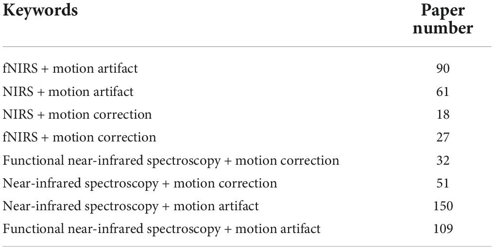
Table 1. The number of journal papers (1990∼2022) obtained from the Web of Science database by combining different keywords.

FIGURE 1

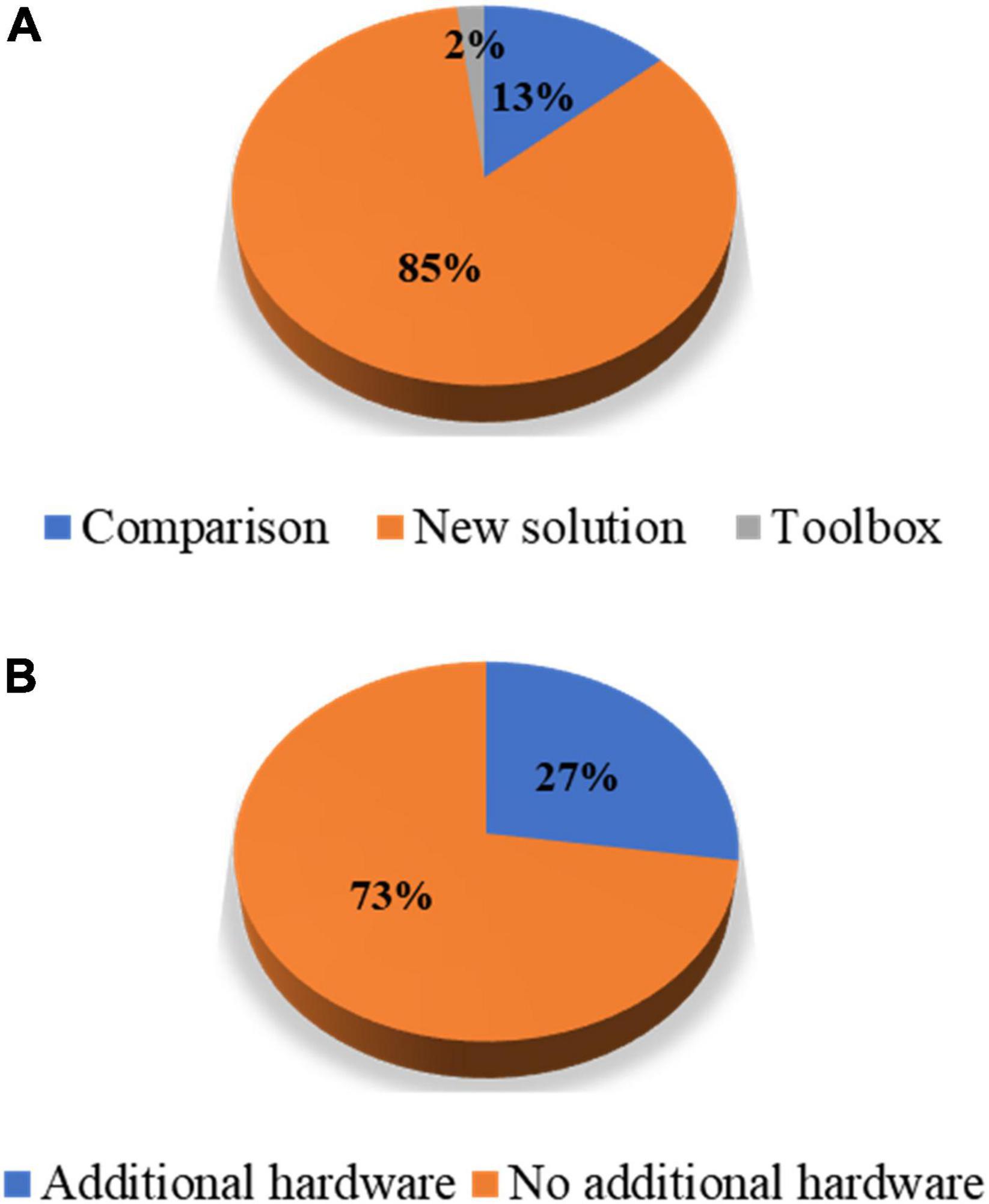
Figure 1. Percentage partitions: (A) Article types of the selected papers and (B) hardware-based solutions against algorithmic solutions among the papers proposing new solutions.

TABLE 2

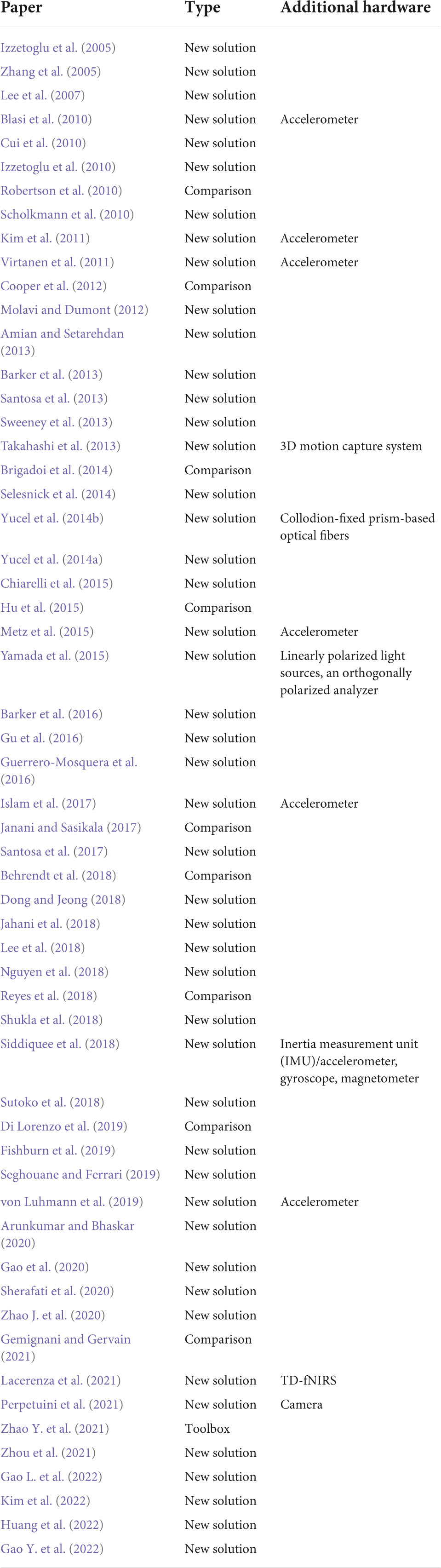
Table 2. List of selected papers, article types, and information on additional hardware.

This study is divided into five sections. The “Introduction” section presents the causes and significance of MA issues in fNIRS. In addition, this section specifies the objectives of this study and provides a quantitative summary of the existing literature on the topics. The section “Additional hardware-based techniques” summarizes the existing hardware-based solutions. The section “Signal processing-based techniques” discusses the algorithmic solutions. The section “Evaluation metrics” briefly introduces the definitions of some metrics to evaluate the performance of MA removal techniques. The final section “Conclusions and outlook” concludes this study and discusses potential issues concerning MA removal. We will use the compact notation provided in Table 3 for the remainder of the paper.

TABLE 3

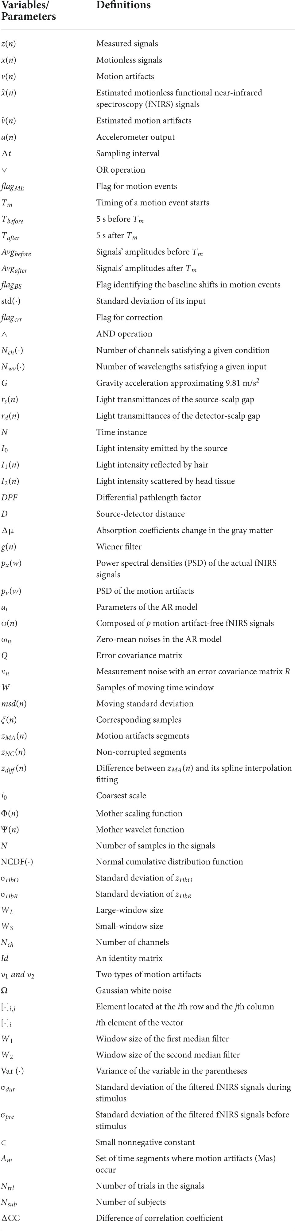
Table 3. Definitions of variables, parameters, and their values.

Additional hardware-based techniques

Among the eight-nine selected papers, 17 discussed solutions using additional hardware, while 11 studies discussed accelerometer-related methods. Other auxiliary hardware includes a headpost cemented to the skull, a three-dimensional (3D) motion capture system, collodion-fixed prism-based optical fibers, an inertia measurement unit (IMU), a gyroscope, a magnetometer, and a camera. This section presents two solutions using accelerometers and one using linearly polarized light.

Accelerometer

Accelerometer-based methods include adaptive filtering, active noise cancelation (ANC) (Kim et al., 2011), accelerometer-based motion artifact removal (ABAMAR) (Virtanen et al., 2011), acceleration-based movement artifact reduction algorithm (ABMARA) (Metz et al., 2015), multi-stage cascaded adaptive filtering (Islam et al., 2017), blind source separation, accelerometer-based artifact rejection, and detection (BLISSA2RD) (von Luhmann et al., 2019). The introduction of the accelerometer improves the feasibility of real-time rejection of MAs.

Active noise cancelation

The method assumes that the measured signals, z(n), are the sum of motionless signals, x(n), and MAs, v(n) (Kim et al., 2011). The objective of the solution is to minimize the power of the recovered signals, that is,

$\min \left(\text{E}\left(\widehat{x}{\left(n\right)}^2\right)\right)=\min \left(\text{E}\left({\left(x\left(n\right)+v\left(n\right)-\widehat{v}\left(n\right)\right)}^2\right)\right)$

$\mathrm{ }=\min (\text{E}\left(x{\left(n\right)}^2\right)+2\text{E}\left(x\left(n\right)v\left(n\right)\right)$

$\mathrm{ }-2\text{E}\left(x\left(n\right)\widehat{v}\left(n\right)\right)+\text{E}\left({(v\left(n\right)-\widehat{v}\left(n\right))}^2\right)).(1)$

where E(⋅) denotes the expectation function, and the hat over x and v denotes the estimation of motionless fNIRS signals and MAs. Ideally, x is uncorrelated to either v or the estimate of v. Therefore, the two cross-terms on the right-hand side are equal to zero implying that the objective is equivalent to minimizing the square difference between the MAs and the estimated MAs. Moreover, because the actual MAs are highly correlated to the accelerometer output, a(n), but unknown to users, v(n) is replaced by a(n) in the application. Subsequently, the final objective of signal processing is to minimize the square difference between a(n) and the estimated MAs, that is,

$\min \left(\text{E}\left({\left(a\left(n\right)-\widehat{v}\left(n\right)\right)}^2\right)\right)(2)$

The estimate of v(n) can be obtained using the difference between z(n) and the estimate of x(n). The estimate of v(n) can then be computed in real time using a recursive least-squares filter. The procedure for the solution is graphically presented in Figure 2. The ANC solution was applied to optical intensities in real time. Whether this method was applied to optical densities or concentration changes is not clear. Another issue in the approach of Kim et al. (2011) is that the performance was visually evaluated. Therefore, a quantitative evaluation of ANC in the sense of both noise suppression and signal distortion is needed.

FIGURE 2

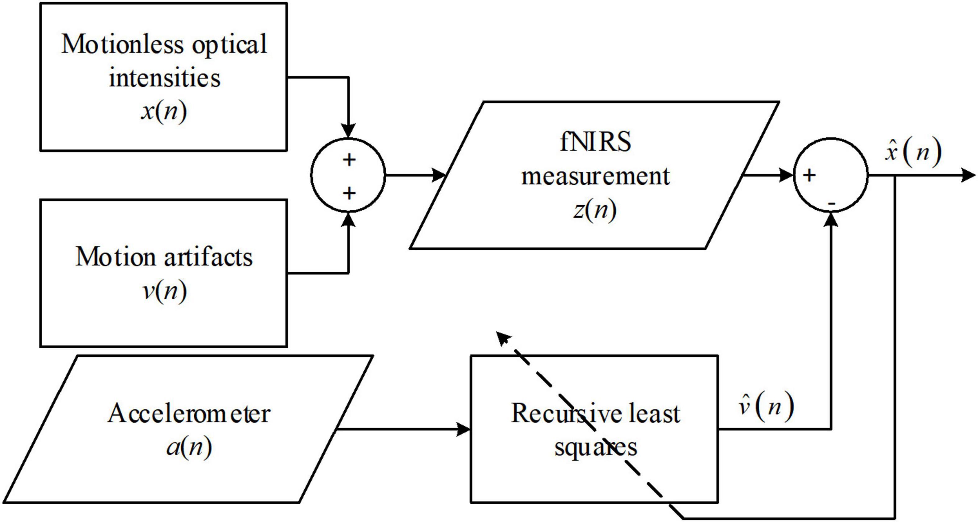
Figure 2. Procedures of active noise cancellation (ANC) algorithm.

Accelerometer-based motion artifact removal algorithm

The ABAMAR method is an offline analysis method for MA removal, where accelerometer outputs are used for MA detection, and the MA removal process is based on the measured fNIRS signals (Virtanen et al., 2011). Accordingly, we first define two Boolean functions as follows.

$f_1\left(x\right)=\{\begin{array}{cc}\hfill 1\hfill & \hfill x\ge 0\hfill \\ \hfill 0\hfill & \hfill x<0\hfill \end{array}(3)$

$f_2\left(x\right)=\{\begin{array}{cc}\hfill 1\hfill & \hfill x>0\hfill \\ \hfill 0\hfill & \hfill x\le 0\hfill \end{array}(4)$

A motion event can then be identified using the acceleration at the x- and y-axes, where Δt is the sampling period. The subscript x or y at a(n) denotes the acceleration at the two axes. The subscript ME denotes the motion event, and operator ∨ denotes the OR operation. The flag for the motion events can be computed as follows.

$fla{g}_{\mathrm{ME}}=f_1\left(\left|a_x\left(n\right)-a_x\left(n-1\right)\right|-1.3\mathrm{\Delta }T\right)\vee f_1\left(\left|a_y\left(n\right)-a_y\left(n-1\right)\right|-1.3\mathrm{\Delta }T\right)(5)$

If flag_ME is one, the signals encounter a motion event; otherwise, zero. Once a first true value of the flag appears, the timing of the motion event starts and is stored/defined as T_m. The motion event is ended when the flag remains false for over 20 s. The ending time is identified as the last sample when flag_ME is true.

Another flag, flag_MA, is introduced to identify the existence of MAs, which is defined as follows.

$fla{g}_{\text{MA}}=f_1\left(T_m-1\right)(6)$

T_m is the starting time of a motion event. The baseline of fNIRS signals, Avg, is defined as the average of the signal amplitudes before and after T_m. To avoid disturbance during the motion event, we marked 5 s before T_m as T_before and 5 s after T_m as T_after. The amplitudes of the signals before T_m, Avg_before, and those after T_m, Avg_after, are calculated as follows.

$Av{g}_{\text{before}}=\text{mean}\left({z\left(n\right)|}_{T_{\text{before}}-15\le n<T_{\text{before}}}\right)(7)$

$Av{g}_{\text{after}}=\text{mean}\left({z\left(n\right)|}_{T_{\text{after}}<n\le T_{\text{after}}+15}\right)(8)$

flag_BS is a flag identifying baseline shifts in motion events. Specifically, one for baseline shifts, and zero for no shift.

$fla{g}_{\text{BS}}=f_2\left(\left|Av{g}_{\text{before}}-Av{g}_{\text{after}}\right|-2.6{\mathrm{\sigma }}_{\text{before}}\right)(9)$

${\mathrm{\sigma }}_{\text{before}}=\text{std}\left({z\left(n\right)|}_{T_{\text{before}}-15\le n<T_{\text{before}}}\right)(10)$

The function std(⋅) computes the standard deviation of its input.

The correction procedure only applies to baseline shift segments. Moreover, a flag for correction, flag_crr, is introduced. If its value is one, a correction of signals will be conducted; otherwise, it is zero. Moreover, operator ∧ denotes the AND operation. The flag_crr can be computed as follows.

$fla{g}_{\text{crr}}=f_1\left(N_{\text{ch}}\left({fla{g}_{\text{BS}}|}_{fla{g}_{\text{BS}}=1}\right)-2\right)\vee f_1\left(N_{\text{wv}}\left({fla{g}_{\text{BS}}|}_{fla{g}_{\text{BS}}=1}-2\right)\right)\mathrm{\wedge }fla{g}_{\text{ME}}(11)$

where N_ch(⋅) denotes the number of channels satisfying the condition specified in the input, and N_wv(⋅) denotes the number of wavelengths satisfying the input. When flag_crr is one, z(n) is corrected as follows.

${\widehat{z}\left(n\right)|}_{n\mathrm{after}{T}_m}=\frac{Av{g}_{\text{before}}}{Av{g}_{\text{after}}}z\left(n\right)(12)$

${\widehat{z}\left(n\right)|}_{n\mathrm{inside}{T}_m}=A_{\text{before}}(13)$

The ABAMAR solution is applied to optical intensities, optical densities, and concentration changes. It can efficiently suppress step-like artifacts. However, the signal details during motion events will be lost owing to the correction method. Moreover, empirical constants, such as 1.3 g/s in Eq. (5) (g denotes the gravitational acceleration of 9.81 m/s²) and 2.6 in Eq. (9), may need to be updated for tasks other than sleeping monitoring. Some researchers have proposed an AMARA, which is an improvement of ABAMAR (Metz et al., 2015), by combining the movement artifact reduction algorithm (MARA; see section “Spline interpolation”) and ABAMAR.

Linearly polarized light-based solution

Multidistance optode arrangement technique

An optical model of light transmission between a source and a detector is developed using light transmittance (Yamada et al., 2015). Here, the light transmittances of the source-scalp gap, detector-scalp gap, and head tissue at time instance n are denoted by r_s(n), r_d(n), and R(n), respectively. Moreover, the light intensity emitted by the source is denoted by I₀, the light intensity reflected by the hair is denoted by I₁(n), and the light intensity scattered by the head tissue is denoted by I₂(n). The optical density can then be computed as follows.

$\mathrm{\Delta }A\mathrm{ }\left(n\right)=-{\displaystyle \frac{I_1\left(n\right)+I_2\left(n\right)}{I_1\left(0\right)+I_2\left(0\right)}}$

$\mathrm{ }=-\log {\displaystyle \frac{I_1\left(n\right)+I_0{r}_s\left(n\right)R\left(0\right)r_d\left(n\right)}{I_1\left(0\right)+I_0{r}_s\left(0\right)R\left(0\right)r_d\left(0\right)}}$

$\mathrm{ }-\log {\displaystyle \frac{I_1\left(n\right)+I_0{r}_s\left(n\right)R\left(n\right)r_d\left(n\right)}{I_1\left(n\right)+I_0{r}_s\left(n\right)R\left(0\right)r_d\left(n\right)}},(14)$

where

$I_0=I_1\left(n\right)+I_2\left(n\right)(15)$

The MA removal solution includes two steps: Step 1 involves suppressing I₁(n), and Step 2 involves attenuating the first term in the model.

Polarized optical films are attached to the source and detector in an orthogonal direction to suppress I₁(n). Light reflection does not change the polarization of light, but scattering will change; therefore, only scattered light can be captured by the detector, that is, I₁(n) = 0. Thus, Eq. (14) can be reduced to the following form:

$\mathrm{\Delta }A\mathrm{ }\left(n\right)=-\log \frac{r_s\left(n\right)r_d\left(n\right)}{r_s\left(0\right)r_d\left(0\right)}-\log \frac{R\left(n\right)}{R\left(0\right)}(16)$

Step 2 is to cancel out the first term because it is independent of the hemodynamic changes. The optode arrangement is depicted in Figure 3. Accordingly, the method assumes that if two unidirectional inline channels have a small distance difference (two sources and one detector), their concentration changes will have similar temporal patterns. The hemodynamic changes contribute to the second term in Eq. (16), so according to the modified Beer–Lambert law, we obtain the following equation:

$-\log \frac{R\left(n\right)}{R\left(0\right)}=DPF\cdot d\mathrm{\Delta }\mu (17)$

FIGURE 3

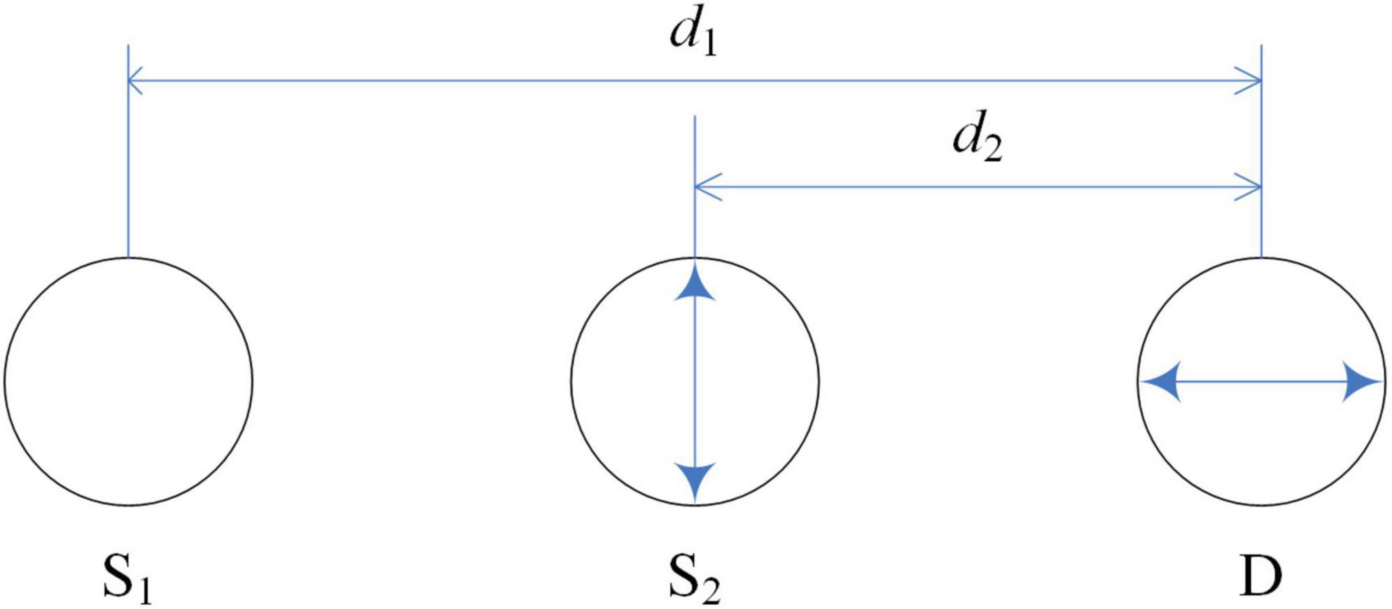
Figure 3. Optode arrangement for multidistance optode arrangement technique.

where DPF denotes the differential pathlength factor, d indicates the source-detector distance, and Δμ corresponds to the absorption coefficient change in the gray matter. Moreover, the light transmittances of the source-scalp gaps for both channels and the detector-scalp gap for the detector are denoted by r_s1(n), r_s2(n), and r_d(n), respectively. R₁(n) and R₂(n) denote the transmittances of the head tissues for the two channels. We can obtain the following equation from Eq. (17) by weighted subtraction of the optical densities of the two channels.

$\mathrm{\Delta }{A}_1\left(n\right)-k\mathrm{\Delta }{A}_2\left(n\right)=-\log {\displaystyle \frac{r_{s1}\left(n\right)r_d\left(n\right)}{{\left(r_{s2}\left(n\right)r_d\left(n\right)\right)}^k}}$

$\mathrm{ }-\log r_{s1}\left(0\right)r_d\left(0\right)+k\log r_{s2}\left(0\right)r_d\left(0\right)$

$\mathrm{ }-\log {\displaystyle \frac{R_1\left(n\right)}{R_1\left(0\right)}}+k\log {\displaystyle \frac{R_2\left(n\right)}{R_2\left(0\right)}}$

$\mathrm{ }=-\log {\displaystyle \frac{r_{s1}\left(n\right)r_d\left(n\right)}{{\left(r_{s2}\left(n\right)r_d\left(n\right)\right)}^k}}$

$\mathrm{ }+C+\left(DP{F}_1{d}_1-kDP{F}_2{d}_2\right)\mathrm{\Delta }\mu \left(n\right).(18)$

The constant k (approximately one) depends on the wavelength, and C is a constant that depends on the initial installation of the device. When the two sources and the detector are fixed relatively well, r_s1(n) and r_s2(n) will be consolidated to a similar value. Thus, the first term tends to be zero.

The solution above was evaluated on a hairy phantom, and its hardware solution in the first step inspired a creative solution to the hair-blocking problem encountered while using fNIRS devices. The validity of the second step is decided by the approximation that k = 1, whereas in actual measurement, k may occasionally become negative (Yamada et al., 2015). Besides, the optical model neglects detection noise and the angular fluctuation of optodes. The multidistance optode arrangement technique is applied to optical density and is available for real-time monitoring. The solution in Step 1 (using polarized optical film) can attenuate hair-reflected light.

Signal Processing-Based Techniques

Wiener filter

The Wiener filter approach is the first to remove motion artifacts without incorporating additional hardware devices (Izzetoglu et al., 2005; Orihuela-Espina et al., 2010; Li L. et al., 2021). The technique assumes that the measured fNIRS signals are a simple addition between the actual fNIRS signals, x(n), and motion artifacts, v(n). Moreover, it is assumed that x(n) and v(n) are stationary and uncorrelated.

$\text{corr}(x\left(n\right),v\left(n\right))=0(19)$

Consequently, the Wiener filter, g(n), minimizes the mean square error between x(n) and $\widehat{x}$(n), that is,

$\min \left(\text{E}\left[e{\left(n\right)}^2\right]\right)=\min \left(\text{E}\left[{\left(x\left(n\right)-\widehat{x}\left(n\right)\right)}^2\right]\right)(20)$

Therefore, the optimum filter can be obtained using the orthogonality principle and simplified using Eq. (19) as follows.

$\text{corr}[e(n),x(n)+v(n)]=\text{corr}[x(n),x(n)]$

$\mathrm{ }-g(n)*\text{corr}[x(n)+v(n),$

$\mathrm{ }x(n)+v(n)]$

$\mathrm{ }=0.(21)$

We obtain the Fourier transform of the Wiener filter by converting Eq. (21) into the frequency domain using the Fourier transform, which is as follows.

$G\left(w\right)=\frac{p_x\left(w\right)}{p_x\left(w\right)+p_v\left(w\right)}(22)$

where p_x(w) and p_v(w) denote the power spectral densities (PSDs) of the actual fNIRS signals and motion artifacts.

In application, a prior experiment is required to determine the PSDs of g(n) by calculating the values of x(n) and v(n). Subsequently, we can determine g(n) on a time scale using the inverse Fourier transform and apply it to new experimental data.

The Wiener filter is the first attempt to remove motion artifacts without a reference signal from additional hardware devices, such as accelerometers. With the g(n) determined, the filter can be implemented for online applications. However, it requires prior knowledge of the PSDs of x(n) and v(n), which makes initial calibration more complex (a particularly designed paradigm is needed). The idea of building the filter model from a prior experiment inspired later research on motion artifact removal techniques.

Kalman filter

The Kalman filter approach was also proposed based on the general idea of the Wiener filter but as a different model (Izzetoglu et al., 2010). The motion artifact-free fNIRS signal, x(n), was modeled using an autoregressive (AR) model. An AR model of order p can be written as

$x(n)=\sum _{i=1}^p{a}_{i}x\left(n-i\right)(23)$

With the motion artifact-free data from the prior experiment, the parameters of the AR model, a_i, i = 1, …, p, can be determined using the Yule-Walker equations. Therefore, the process equation for the Kalman filter has the following form.

$\text{ϕ}\left(n\right)=A\text{ϕ}\left(n-1\right)+{\text{ω}}_n,\text{ϕ}\left(n\right)={\left[\begin{array}{c}\hfill x\left(n\right)\mathrm{ }\text{⋯}\mathrm{ }x\left(n-p+1\right)\hfill \end{array}\right]}^T(24)$

where ϕ(n) is composed of p motion artifact-free fNIRS signals, and ω_n denotes the zero-mean noises in the AR model with an error covariance matrix Q. Matrix A can be obtained using Eq. (23) as follows.

$A=\left[\begin{array}{cccc}\hfill a_1\hfill & \hfill \text{⋯}\hfill & \hfill a_{p-1}\hfill & \hfill a_p\hfill \\ \hfill 1\hfill & \hfill \text{⋯}\hfill & \hfill 0\hfill & \hfill 0\hfill \\ \hfill \mathrm{⋮}\hfill & \hfill \text{⋯}\hfill & \hfill \text{⋯}\hfill & \hfill \mathrm{⋮}\hfill \\ \hfill 0\hfill & \hfill \text{⋯}\hfill & \hfill 1\hfill & \hfill 0\hfill \end{array}\right](25)$

The measurement equation can be written as follows.

$z\left(n\right)=C\text{ϕ}\left(n\right)+{\mathrm{\nu }}_n(26)$

$C=\underset{p\mathrm{elements}}{\underbrace{\left[\begin{array}{cccc}\hfill 1\hfill & \hfill 0\hfill & \hfill \text{⋯}\hfill & \hfill 0\hfill \end{array}\right]}}(27)$

where ν_n denotes the measurement noise (such as the motion artifact) with an error covariance matrix R. z(n) denotes the motion artifact corrupted signal.

Subsequently, Eqs. (24) and (26) form the state-space model for the Kalman filter, see Table 4. The minus sign in the superscript denotes the prior estimate of a variable. Subsequently, the motion-free fNIRS signal can be obtained using the Kalman filter (Wan and Nelson, 2001). The Kalman filter method can be applied to any online application of optical intensities, optical densities, and concentration changes, and in the Kalman filter theory, both ω_n and ν_n are assumed to be zero-mean Gaussian white noise (Huang and Hong, 2021; Haghighi and Pishkenari, 2021; Li B. A. et al., 2021; Sun and Zhao, 2021; Yang et al., 2021; Lv et al., 2021; Tang et al., 2020; Pham et al., 2021). However, it is not the case for ν_n (motion artifacts do not observe the zero-mean Gaussian distribution). It may degrade the filter’s performance (Zhou et al., 2017). Moreover, matrices A and C were fixed once determined by the Yule-Walker method. Therefore, further development of the algorithm focuses on; (i) the compensation of the instrumental noises (Amian and Setarehdan, 2013) and (ii) adaptive adjustment of A and C, or using a more sophisticated and nonlinear model in place of Eqs. (24) and (26) (Dong and Jeong, 2018).

TABLE 4

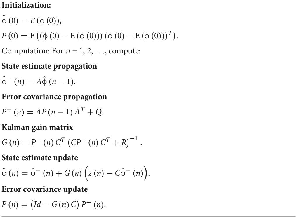
Table 4. Kalman filter algorithm.

Additionally, the state-space model for the Kalman filter method is not unique. A typical example is the incorporation of the autoregressive iterative robust least-squares model (AR-IRLS), the general linear model (GLM), and two linear Kalman filters (Barker et al., 2016). A GLM and an AR-IRLS replaced the state-space model in the Kalman filters. The GLM was introduced to describe the dynamics of hemodynamic responses and physiological noises. The AR-IRLS was introduced as compensation for the MAs in the signals. A difference between the GLM-based method and the AR model-based method is that the GLM-based method requires the information of experimental paradigms, while the AR model-based method does not. Despite the significant adaptation ability of the Kalman filter regarding its state-space model, its applications are limited due to the effort required to set its initial parameters (e.g., the error covariance matrices for the state and the observation).

Spline interpolation

The spline interpolation method was first proposed by Scholkmann’s group and is referred to as the MARA (Scholkmann et al., 2010; Selb et al., 2015; Lee et al., 2021). The method made two fundamental assumptions: (i) The measured fNIRS signal is a linear addition of the motion artifacts and the motion-free fNIRS signal, and (ii) in the motion-corrupted segments in the signal, the motion artifact component dominates the measured fNIRS signal. Therefore, the proposed MARA comprised two parts: (i) Motion artifact detection and segmentation, and (ii) motion artifact removal. A flowchart of MARA is illustrated in Figure 4. The spline interpolation method encompasses six processing steps. First, the moving standard deviation (MSD) is calculated within a moving time window of W samples and stored as msd(n).

$msd\left(n\right)={\displaystyle \frac{1}{W}}\sqrt{{\displaystyle \sum _{i=-k}^k}n+i-{\displaystyle \frac{1}{W}}{\left({\displaystyle \sum _{i=-k}^k}z\left(n+i\right)\right)}^2},W=2k+1,k\in {\mathbb{N}}^{*}(28)$

FIGURE 4

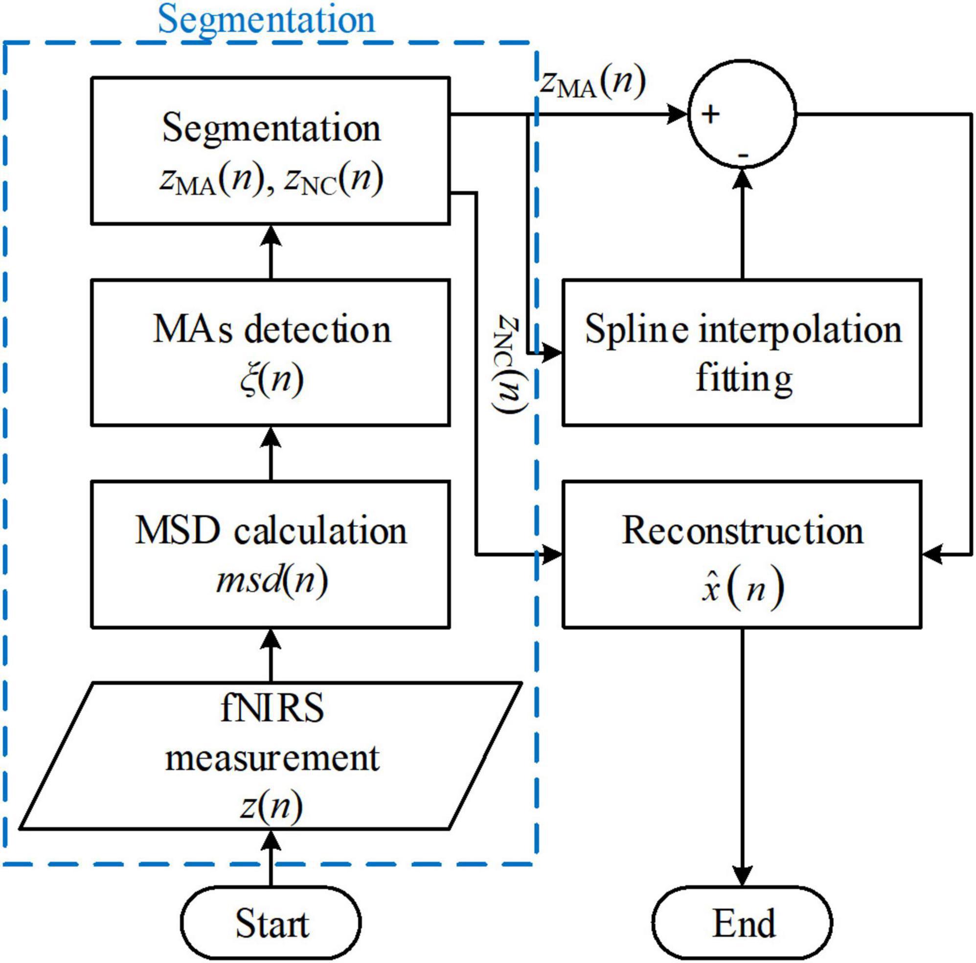
Figure 4. Flowchart of the movement artifact reduction algorithm (MARA) algorithm. The process blocks in the blue box are one of the reasons that limit the solution’s online application.

where N* is the set of natural numbers.

We can determine the start and end points of the motion artifacts and store the indices of the corresponding samples in a vector ξ(n) by comparing with the MSD [i.e., msd(n) in Eq. (28)] with a user-defined threshold value T. If the MSD is smaller than T, the corresponding msd(n) will be assigned as zero. The start points and endpoints of motion artifacts can be extracted by considering the first and last samples of non-zero values in msd(n). Next, let us suppose that there are L segments of motion artifacts and let the motion artifact segments, z_MA(n), and the non-corrupted segments, z_NC(n), be expressed, respectively, as

$z_{\text{MA}}\left(n\right)=\{z_{\text{MA},1}\left(n\right),\text{⋯},z_{\text{MA},L}\left(n\right)\}(29)$

$z_{\text{NC}}\left(n\right)=\{z_{\text{NC},1}\left(n\right),\text{⋯},z_{\text{NC},L}\left(n\right)\}(30)$

Using Eqs. (29) and (30), the measured fNIRS signals can be segmented into non-corrupted segments and motion artifact segments.

In the next part, the spline interpolation method corrects motion artifact segments. Because the motion artifact components dominate the MA segments, the spline interpolation fitting of z_MA(n) can be viewed as the motion artifact component. The difference between z_MA(n) and its spline interpolation fitting is stored as z_diff(n):

$z_{\text{diff}}\left(n\right)=\{z_{\text{diff},1}\left(n\right),\text{⋯},z_{\text{diff},L}\left(n\right)\}(31)$

Because z_NC(n) and z_diff(n) may have different magnitude levels, the final step involves correcting the signal levels for the entire time series. Each segment is parallel-shifted according to the mean of the previous segment and that of the target segment. Two empirical constant thresholds, α = 3^–1 Hz^–1⋅fs and β = 2 Hz^–1⋅fs (where the variable fs denotes the sampling frequency), were chosen for comparison. The detailed shifting rules are listed in Table 1 in Scholkmann et al. (2010).

The spline-interpolation method is used widely for offline analysis in fNIRS studies. It has also been included in some open-source toolboxes, such as HomER2 and NIRSLAB (Balardin et al., 2017). Moreover, the method applies not only to the optical intensities and optical densities but also to concentration changes. However, both the segmentation procedure (the procedures in the blue box in Figure 4) and the parallel-shifting procedure (in the reconstruction process) increase the difficulty for online filtering applications. Moreover, the filter performance depends on artifact detection results (Brigadoi et al., 2014). Some variations of the spline interpolation method have also been proposed (Jahani et al., 2018; Zhou et al., 2021).

Wavelet-based method

The wavelet-based method eradicates motion artifacts by removing the corresponding wavelet coefficients (Molavi and Dumont, 2012; Pinti et al., 2015), without requiring auxiliary devices. The method made the same assumption as the Wiener filter case, that is, z(n) = x(n) + v(n). Based on discrete wavelet transform (DWT), fNIRS signals can be expanded as follows.

$z\left(n\right)=\sum _k{a}_{i_{0}k}{\mathrm{\phi }}_{i_{0}k}\left(n\right)+\sum _{i=i_0}^{\mathrm{\infty }}\sum _k{b}_{ik}\mathrm{\psi }\left(n\right)(32)$

where i denotes the dilation parameter, k indicates the translation parameter, and i₀ denotes the coarsest scale. The scaling function φ_i0k and the wavelet function ψ_ik are as follows.

${\mathrm{\phi }}_{i_{0}k}\left(n\right)=2^{i_0/2}\mathrm{\Phi }\left(2^{i_0}n\text{-}k\right)(33)$

${\mathrm{\psi }}_{ik}\left(n\right)=2^{i/2}\mathrm{\Psi }\left(2^{i}n\text{-}k\right)(34)$

The functions Φ(n) and Ψ(n) correspond to the mother scaling function and mother wavelet function, respectively. With the fast wavelet transform, the coefficients of the DWT of z(n) become

$a_{i_{0}k}=\sum _{l=0}^{N-1}h\left(l-2k\right)z\left(l\right),k=0,\mathrm{\dots }\mathrm{ },2^i-1(35)$

$b_{ik}=\sum _{l=0}^{N-1}g\left(l-2k\right)z\left(l\right),i=i_0,\mathrm{\dots }\mathrm{ },J-1(36)$

where N denotes the number of samples in the signal and N = 2^J. g(n) and h(n) denote the wavelet filter bank high- and low-pass filters, respectively. Therefore, Eqs. (35) and (36) can be written in the matrix form as follows.

$W=\text{Ω}Z,Z={\left[z\left(0\right)\mathrm{ }\text{…}\mathrm{ }z\left(N-1\right)\right]}^T(37)$

where W = [B₁, B₂, …, B_J–1, A_i0]^T, B_i = [b_i0, …, b_i(2∧i–1)], A_i0 = [a_i00, …, a_{i0(2∧i0–1)}]. Ω is an N by N DWT matrix. For any element w_ik in the wavelet coefficient vector W, the probability of observing its value can be written as

$p_{ik}=2\left(1-NCDF\left(\frac{\left|w_{ik}\right|}{\widehat{\mathrm{\sigma }}}\right)\right)(38)$

where NCDF(⋅) is a normal cumulative distribution function. The estimated standard deviation of w_ik can be approximated empirically as

${\widehat{\mathrm{\sigma }}}_i=\frac{\text{Median}\left(\left|W_i\right|\right)}{0.6745}(39)$

where W_i denotes B_i or A_i0 according to the value of i. Given a probability threshold α, if p_ik < α, we consider that the corresponding wavelet coefficient w_ik is dominated by artifacts and set to zero. The filtered signals can be obtained from the updated wavelet coefficient vector as

${\left[\widehat{x}\left(0\right)\mathrm{ }\text{…}\mathrm{ }\widehat{x}\left(N-1\right)\right]}^T={\text{Ω}}^T\widehat{W}(40)$

The hat over x(⋅) denotes the filtered fNIRS signal, and the hat over W denotes the updated wavelet coefficient vector after thresholding.

Similar to the spline interpolation method, the wavelet-based method can be applied to optical intensities, optical densities, and concentration changes. Initially, the wavelet-based method was first introduced as an offline artifact removal algorithm. It may be adjusted to be an online method using the windowing technique; however, its filtering performance will be degraded. Several variations of this method have also appeared in recent years (Chiarelli et al., 2015; Shukla et al., 2018; Perpetuini et al., 2021). Gao Y. et al. (2022) addressed that the tuning of the probability threshold is crucial, and Wei et al. (2018) designed a dual-threshold structure to improve the performance of the wavelet-based method.

Correlation-based signal improvement method

Based on the negative correlation between measured oxyhemoglobin (HbO) and deoxyhemoglobin (HbR) concentrations, the correlation-based signal improvement (CBSI) method was proposed in 2010 (Cui et al., 2010; Haeussinger et al., 2014). The algorithm made three fundamental assumptions: (i) HbO concentrations are strictly negatively correlated with HbR concentrations (close to –1); (ii) motion artifacts have identical effects on HbO and HbR, subject to a constant factor; and (iii) motion artifacts are not correlated to the actual concentration changes. The measured concentration changes were modeled as follows.

$\begin{array}{c}{z}_{\text{HbO}}\left(n\right)=x_{\text{HbO}}\left(n\right)+\mathrm{\chi }v,\hfill \\ z_{\text{HbR}}\left(n\right)=x_{\text{HbR}}\left(n\right)+v,\hfill \end{array}(41)$

where v denotes the motion artifact of the HbR signals, and χ is a constant. Based on the first assumption, we can reasonably obtain

$x_{\text{HbO}}\left(n\right)=-\beta x_{\text{HbR}}\left(n\right)(42)$

β denotes the free ratio accounting for the magnitude difference between HbO and HbR. Equations (41) and (42) can be used to obtain the following:

$\begin{array}{c}v\left(n\right)=\frac{z_{\text{HbO}}\left(n\right)+\beta z_{\text{HbR}}\left(n\right)}{\mathrm{\chi }+\beta },\hfill \\ x_{\text{HbO}}\left(n\right)=\frac{\beta }{\mathrm{\chi }+\beta }\left(z_{\text{HbO}}-\mathrm{\chi }{z}_{\text{HbR}}\right).\hfill \end{array}(43)$

Based on the third assumption, we set the correlation between v and x_HbO to zero, yielding

${\displaystyle \sum _n}{z}_{\text{HbO}}{\left(n\right)}^2+\left(\beta -\mathrm{\chi }\right){\displaystyle \sum _n}{z}_{\text{HbO}}\left(n\right)z_{\text{HbR}}\left(n\right)-\mathrm{\chi }\beta {\displaystyle \sum _n}{z}_{\text{HbR}}{\left(n\right)}^2=0(44)$

We assumed that χ = β. Then, Eq. (44) can be reduced to

$\mathrm{\chi }=\frac{{\mathrm{\sigma }}_{\text{HbO}}}{{\mathrm{\sigma }}_{\text{HbR}}}(45)$

where σ_HbO and σ_HbR denote the standard deviations of z_HbO and z_HbR, respectively. Therefore, the final CBSI filter is

$\begin{array}{c}{x}_{\text{HbO}}\left(n\right)=\frac{1}{2}\left(z_{\text{HbO}}\left(n\right)-\mathrm{\chi }{z}_{\text{HbR}}\left(n\right)\right),\hfill \\ x_{\text{HbR}}\left(n\right)=-\frac{1}{\text{α}}{x}_{\text{HbO}}\left(n\right).\hfill \end{array}(46)$

Once χ is decided based on prior-experimental data, the CBSI filter can be easily implemented for online applications using Eq. (46). As mentioned in (Cui et al., 2010), CBSI can be applied after an exponential moving average (EMA) filter to facilitate real-time analysis. The behavior of an EMA filter is similar to an online version of a band-pass filter. The EMA is described as follows.

$\begin{array}{c}L\left(n\right)=\frac{1}{W_{\text{L}}}z\left(n\right)+\left(1-\frac{1}{W_L}\right)L\left(n-1\right),\hfill \\ S\left(n\right)=\frac{1}{W_{\text{S}}}{\sum }_{k=0}^{W_s}z\left(n-k\right),\hfill \\ x\left(n\right)=S\left(n\right)-L\left(n\right).\hfill \end{array}(47)$

L(n) denotes the signal filtered by a large-window moving average (window size as W_L), and S(n) denotes the signal filtered by a moving average of window size W_S.

Owing to the fundamental assumptions of the filter, the CBSI filter can only be applied to concentration changes. However, the negative correlation assumption between the HbO and HbR concentrations may not always be true for experimental data. Typically, the CBSI method is used for comparison in the literature (Janani and Sasikala, 2017; Reyes et al., 2018; Sherafati et al., 2020).

Principal component analysis

The solution based on principal component analysis (PCA) was developed from a multivariate method to remove physiological noises. The PCA-based method, entitled targeted PCA (tPCA), is similar to spline interpolation, except for using PCA instead of spline interpolation to fit the noisy segments in the signals (Yucel et al., 2014a). In this subsection, we subsequently explain the mechanism of Zhang’s method and tPCA.

In accordance with the regular PCA method, the systemic spatial interference subspace (the actual hemodynamic responses) dominates in the baseline over the measured concentration changes and it spans during the stimulation periods for the first few components. The measured fNIRS signals are first converted to HbO and HbR concentration changes and are band-pass filtered. The filtered data from a chosen channel set are formatted into two N_ch × N matrices, Z_HbO and Z_HbR, where N_ch denotes the number of channels and N is the number of time samples. When segmented into two parts according to the baseline and stimulation periods, the two matrices turn out to be as follows.

$Z_{\text{HbO}}=\left[\begin{array}{cc}\hfill Z_{\text{HbO},\text{base}}\hfill & \hfill Z_{\text{HbO},\text{stim}}\hfill \end{array}\right](48)$

$Z_{\text{HbR}}=\left[\begin{array}{cc}\hfill Z_{\text{HbR},\text{base}}\hfill & \hfill Z_{\text{HbR},\text{stim}}\hfill \end{array}\right](49)$

For simplification, we omit the subscripts HbO and HbR, primarily because the filtering operations are identical for both chromophores. Accordingly, the spatial correlation matrices for the baseline signals are as follows.

$C_{\text{base}}=1/N\cdot Z_{\text{base}}{Z}_{\text{base}}^T(50)$

The eigen-values and the eigenvectors can be obtained by the eigen-decomposition of spatial correlation matrices:

$C_{\text{base}}=U_{\text{base}}{\mathrm{\Sigma }}_{\text{base}}{U}_{\text{base}}^T(51)$

where the rows of U_base contains the eigenvectors, and Σ_base contains the eigenvalues in its diagonal. Based on the dominant interference subspace assumption, we assume that the first r spatial eigenvectors span in the stimulation period as U_base,r, an N_ch by r matrix padding by zeros. Accordingly, the actual hemodynamic responses will be the projection of the measured fNIRS signals onto the orthogonal subspace of the first r eigenvectors. The superscript ^⊥ denotes the orthogonal subspace. Then, the filtered fNIRS signals were

$X_{\text{stim}}=\left(Id-U_{\mathrm{base},r}{U}_{\mathrm{base},r}^T\right)Z_{\text{stim}}=U_{\mathrm{base},r}^{\perp }{U}_{\mathrm{base},r}^{\perp T}{Z}_{\text{stim}}(52)$

where X_stim denotes the filtered fNIRS signal and matrix Id is an N_ch by N_ch identity matrix. Finally, we can block the average X_stim around the stimulus to improve the signal-to-noise ratio (SNR).

To remove MAs, tPCA applies the multivariate PCA method on MA segments. The eigenvectors in U_base are ranked in decreasing order of the percent variance of eigenvalues in Σ_base. The number of spatial eigenvectors span, r, is the minimum integer obtaining not less than 97% percent variance. Then, the filtered fNIRS signals of the segments are stitched back into the original signals after shifting the average of adjacent data segments (identical to MARA). The processing procedures are repeated twice or three times until there is no further improvement in the results.

Targeted PCA applies to optical densities. Due to the iteration in MA identification, the method cannot apply to online filtering. tPCA can remove both spike-like MAs and baseline shifts. It can better suppress high-frequency MAs than MARA (Yucel et al., 2014a). However, during application, the performance of tPCA may degrade if the MAs are not present in multiple channels (Brigadoi et al., 2014). The method requires multiple channels, which is not an appropriate choice when the number of channels is limited.

Multi-channel regression

The idea of the method is to subtract a best-fit linear combination of the noise references from each signal (Robertson et al., 2010). For a k-channel regression, the measured signal is modeled as follows.

$z=aH+x(53)$

where z ϵ ℝ^{1 × N}, a ϵ ℝ1 × k, H ϵ ℝ^{(k + 1) ×N}, x ϵ ℝ^{1 × N}. The row vector, a, is the weight for each reference channel in H. The regressor H is defined as follows.

$H=\left[\begin{array}{ccc}\hfill 1\hfill & \hfill \text{⋯}\hfill & \hfill 1\hfill \\ \hfill z_{r1}\left(1\right)\hfill & \hfill \text{⋯}\hfill & \hfill z_{r1}\left(N\right)\hfill \\ \hfill \mathrm{⋮}\hfill & \hfill \mathrm{⋮}\hfill & \hfill \mathrm{⋮}\hfill \\ \hfill z_{rk}\left(1\right)\hfill & \hfill \text{⋯}\hfill & \hfill z_{rk}\left(N\right)\hfill \end{array}\right](54)$

where z_ri (i = 1, 2, …, k) is the measurement of the ith reference channel. It is recommended to take co-located channels as reference channels in priority. Therefore, a can be estimated using the least-squares method.

$a={\left(H^{T}H\right)}^{-1}{H}^{T}z(55)$

The motionless signal, x, can be obtained by subtracting aH from z.

The multi-channel regression method does not require an auxiliary device and applies to optical intensities, optical densities, and concentration changes. It was first designed as an offline filtering method, but it can apply to online applications simply by replacing the least-square estimation procedure with recursive least-square estimation. When different types of artifacts affect collocated channels differently, the multi-channel regression method may not remove MAs entirely.

Independent component analysis

Independent component analysis (ICA) can decompose a signal to the weighted sum of multiple independent sources statistically (Kohno et al., 2007; Santosa et al., 2013). Therefore, the ICA solutions belong to blind source separation methods (von Luhmann et al., 2019). The key to removing MAs using ICA is how to select the components relevant to motionless signals or MAs. Kohno et al. (2007) suggested identifying the components related to artifacts using the coefficient of spatial uniformity (CSU).

$CS{U}_j=\left|\frac{{\overline{s}}_j}{\text{std}\left(s_j\right)}\right|(56)$

Additionally, Santosa et al. (2013) estimated motionless signals by weighted reconstructing from independent components according to the t-values between each component and the desired hemodynamic response. The desired hemodynamic response is the convolution between the canonical hemodynamic response and the experimental paradigm (a boxcar function).

The ICA applies to optical intensities, optical densities, and concentration changes. The input requirements may vary according to the reconstruction strategy. Some researchers concluded that the performance of ICA was not satisfactory in some applications because fNIRS signals contained both non-instantaneous and non-constant coupling, correlated noise, and source dependencies (von Luhmann et al., 2019).

Temporal derivative distribution repair

The temporal derivative distribution repair (TDDR) is an online filtering method based on the temporal derivative of fNIRS signals. Three basic assumptions were made for this method: Non-motion fluctuations are assumed to be normally distributed; most fluctuations are independent of motion artifacts; and the derivatives of motion artifacts dominate in the derivatives of fNIRS signals when they are present (Fishburn et al., 2019). Therefore, the algorithm can be divided into five steps.

Step 1: For time instance n, the variation in the fNIRS signal can be calculated as follows.

$Dz\left(n\right)=z\left(n\right)-z\left(n-1\right)(57)$

where the D before z(n) denotes the temporal derivative of the measured signal at instance n.

Step 2: The observation weight w(n), corresponding to Dz(n), is initialized as one.

Step 3: The observation weight is adaptively updated using a robust estimator, M-estimator, and Tukey’s biweight function:

$w\left(n\right)=\{\begin{array}{cc}\hfill {\left(1-{\mathrm{\sigma }}_s{\left(n\right)}^2\right)}^2\hfill & \hfill {\mathrm{\sigma }}_s\left(n\right)<1,\hfill \\ \hfill 0\hfill & \hfill \mathrm{otherwise},\hfill \end{array}(58)$

where σ_s(n) denotes the scaled deviation at instance n. An estimate of σ_s(n) can be obtained from the weighted mean of the fluctuations, the absolute residuals of the temporal derivative, and the median absolute residual scale for the normal distribution. Let μ denote the weight mean of fluctuations, res(n) denote the absolute residuals of temporal derivatives, and σ(n) represent the median absolute residuals scale. Subsequently, we can obtain the following:

$\mathrm{\mu }=\frac{1}{{\sum }_{i=1}^{n}w\left(i\right)}\sum _{i=1}^{n}w\left(i\right)Dz\left(i\right)(59)$

$res\left(n\right)=\left|Dz\left(n\right)-\mathrm{\mu }\right|(60)$

$\mathrm{\sigma }=1.4826\cdot \text{median}\left(res\right)(61)$

Repeat (54)–(57) and consider σ_s(n) = σ(n) until μ converges.

Step 4: The filtered temporal derivative can be obtained using μ and w(n) obtained in Step 3.

$Dx\left(n\right)=w\left(n\right)\left(Dz\left(n\right)-\mathrm{\mu }\right)(62)$

Step 5: The final filtered signal is the integration of corrected temporal derivatives.

$x\left(n\right)=\sum _{i=1}^{n}Dx\left(n\right)(63)$

Importantly, the filter can be implemented offline and online. The only difference is that when implemented online, the sum of w(n) and w(n)Dz(n) should be stored in each loop to facilitate the calculation in Eq. (59). The TDDR algorithm can be used for concentration changes, optical intensities, and optical densities. The performance and computation time of the TDDR depend on the convergence criterion in Step 3. In particular, in Eq. (61), the iterative application of the median operator may result in a significant computation time. Furthermore, as the total number of data increases, the computation time increases according to regarding the complexity of the sorting algorithm in the median filter. Fishburn’s group claimed that 130 ms were required to process a dataset of 20 Hz (50 ms in period) (Fishburn et al., 2019). A long computation time may lead to a loss in data transfer or a delay in the data output. In addition, high-frequency noise may degrade the performance of TDDR.

Transient artifact reduction algorithm

The transient artifact reduction algorithm (TARA) is an offline artifact removal method. The algorithm attempts to estimate motion artifacts instead of filtering the original signal directly (Selesnick et al., 2014). Generally, motion artifacts can be divided into two types. The Type 1 artifacts are modeled as spikes, whereas Type 2 artifacts are modeled as additive step shapes. The corrupted fNIRS signals were modeled as a low-pass filter/compound noise denoising problem (LPF/CSD).

$z=x+{\mathrm{\nu }}_1+{\mathrm{\nu }}_2+\text{ω}(64)$

where ν₁ and ν₂ denote the two types of MAs, and ω denotes the Gaussian white noise. Besides, the desired uncorrupted fNIRS signal x is assumed to approximate an all-zero signal when filtered by an appropriately chosen high-pass filter, denoted by HF. Accordingly, when designed as a zero-phase recursive discrete-time filter, H can be factorized into matrices A and B such that

$HF=B{A}^{-1}(65)$

The first-order difference operator matrix D is defined as follows.

$D=\underset{N\mathrm{elements}}{\underbrace{\left[\begin{array}{ccccc}\hfill -1\hfill & \hfill 1\hfill & & & \\ & \hfill -1\hfill & \hfill 1\hfill & & \\ & & \hfill \mathrm{\ddots }\hfill & \hfill \mathrm{\ddots }\hfill & \\ & & & \hfill -1\hfill & \hfill 1\hfill \end{array}\right]}}(66)$

Inversely, the discrete-time integrator S is defined as the matrix satisfying DS = Id_{N × N}, where Id_{N × N} indicates an N by N identity matrix. Then, matrix B can be further factorized as

$B=B_{1}D(67)$

Subsequently, we can change the variables using the following equations.

${\mathrm{\nu }}_1=A{u}_1(68)$

${\mathrm{\nu }}_2=SA{u}_2(69)$

Type 2 MAs are expressed in Eq. (69) because their first-order difference resembles Type 1 artifacts.

The two types of artifacts can be estimated using the following procedures when the factorization matrices A and B for the desired high-pass filter, two weight parameters λ₁ and λ₂, and two penalty functions r₀, r_1, and r₂ are available.

Step 1: Input fNIRS signals z, three regularization parameters λ₀, λ₁, and λ₂, penalty functions r₁ and r₂, and factorization matrices A and B for the desired high-pass filter (they can be calculated from a given degree, cutoff frequency, and length of z).

Step 2: The first additive terms for the estimator for both types of artifacts are as follows.

$z_1=B^{T}B{A}^{-1}z(70)$

$z_2=B_1^{T}B{A}^{-1}z(71)$

The vectors u₁ and u₂ will be initialized as zero vectors.

Step 3: Repeat the following calculation until u₁ and u₂ converge.

${\left[{\mathrm{\Lambda }}_0\right]}_{n,n}={\text{λ}}_0/{\mathrm{\psi }}_0\left({\left[A{u}_1\right]}_n\right)(72)$

${\left[{\mathrm{\Lambda }}_1\right]}_{n,n}={\text{λ}}_1/{\mathrm{\psi }}_1\left({\left[DA{u}_1\right]}_n\right)(73)$

${\left[{\mathrm{\Lambda }}_2\right]}_{n,n}={\text{λ}}_2/{\mathrm{\psi }}_2\left({\left[A{u}_2\right]}_n\right)(74)$

$Q_1=2B^{T}B+A^T\left({\mathrm{\Lambda }}_0+D^T{\mathrm{\Lambda }}_{1}D\right)A(75)$

$Q_2=2B_1^T{B}_1+A^T{\mathrm{\Lambda }}_{2}A(76)$

$g=B{u}_1-B_1{u}_2(77)$

$u_1=Q_1^{-1}\left(z_1+B^{T}g\right)(78)$

$u_2=Q_2^{-1}\left(z_2+B_1^{T}g\right)(79)$

where Λ_i, (i = 0, 1, or 2) is diagonal, ψ_i = u_i/r_i’, [⋅]_i,j denotes the element located at the ith row and jth column of the matrix, and [⋅]_i denotes the ith element of the vector. The superscript prime notation, ′, is the derivative operator.

Step 4: The estimated artifacts can be obtained using Eqs. (68) and (69). Accordingly, the filtered fNIRS signals becomes the following.

$x=z-{\mathrm{\nu }}_1-{\mathrm{\nu }}_2(80)$

The TARA method is applied to optical densities, optical intensities, and concentration changes. TARA exhibits a similar performance to the wavelet-based method but is better at removing Type 2 motion artifacts. TARA is limited to Type 1 and Type 2 artifacts but is not designed for oscillatory transients.

Dual-stage median filter

The dual-stage median filter (DSMF) method resembles an online method for motion artifact removal (Huang et al., 2022). Similar to the TARA, the design of a DSMF is based on Type 1 and Type 2 artifact categories.

The measured fNIRS signal, z, is first filtered using the first median filter with a window size of W₁.

$x_1={\text{median}}_{W_1}\left(z\right)(81)$

Subsequently, the difference between z and x₁ is filtered using the second median filter with a window size of W₂.

$x_2={\text{median}}_{W_2}\left(z-x_1\right)(82)$

The output of the second median filter conserves the variations in the uncorrupted signals; however, it is biased. Therefore, the final step involves compensation of the bias using the initial time point.

$x=x_2+z\left(0\right)(83)$

W₁ can be set as 8 s, while W₂ as 18 s.

The DSMF is applied to optical intensities, optical densities, and concentration changes. Unlike the TDDR method, although two median filters are used in the algorithm, they are called once within fixed window sizes for each estimate. Moreover, registers can store the sorted data sequence during real-time applications, thereby reducing computation time. Therefore, a long computational time problem can be solved relatively quickly. Similar to the TARA, the DSMF is not designed for oscillatory transients.

Convolution neural networks

The convolution neural network (CNN) was adopted for MA removal in 2022 (Gao Y. et al., 2022; Kim et al., 2022). The denoising auto-encoder (DAE) model adopted a serial structure incorporating max-pooling and up-sampling layers (Gao Y. et al., 2022). The model enabled an offline MA removal by minimizing the linear combination of mean square error (L_mse), variance (L_var), standard deviation (L_std), and amplitude loss (L_amp).

$Loss=L_{\text{mse}}+{\theta }_1\times L_{\text{var}}+{\theta }_2\times L_{\text{std}}+{\theta }_3\times L_{\text{amp}}(84)$

where θ₁, θ₂, and θ₃ were set as 1, 1, and 10. The model parameters were estimated using simulated data generated from experimental data in the training process. The CNN structure is shown in Figure 1 of the reference (Gao Y. et al., 2022).

Kim et al. (2022) adopted the CNN in the U-net structure for offline MA removal. Different from the DAE model, the U-net structure accepted an input containing two feature channels.

$u\left(k\right)=\left[z\left(k\right)\mathrm{ }dHR\left(k\right)\right]\in {ℝ}^{N\times 2},k\in \{1,2,\text{…}\mathrm{ },J\}(85)$

where u(k) is the input of U-net of the kth package, J is the total number of packages, and dHR(k) is the desired hemodynamic response of the kth package. dHR(k) is the convolution between a canonical hemodynamic response function and a stimulus function.

$dHR\left(k\right)=cHR*stim\left(k\right)(86)$

The U-net solution adopted the mean square errors between the ground-truth motionless fNIRS signals and the estimated signals as its loss function in the training process. The configurations of the U-net structure are shown in Figure 1 of the reference (Kim et al., 2022).

The DAE model can be applied to optical intensities for offline filtering. It takes measured data in a full-time sequence, outputs the estimated motionless signals, and is trained using simulated data from an AR model. Therefore, the quality of the simulated data has a significant impact on the filtering performance of the model.

In contrast, the U-net structured CNN was applied to concentration changes. The training dataset was obtained through a semi-simulation process, and the size of each package was fixed as 1,024 samples. If the fNIRS data are obtained at a low sampling frequency, the package size is sufficient, but the filtering performance for high-sampling-frequency fNIRS data remains unknown. The matrix structure of the input data enables an easy adaptation to fNIRS measurement with multi-distance configurations. However, similar to the GLM-based method, the information of the stimulation paradigm is a prerequisite in the input. The inclusion of the stimulation paradigm is critical to obtain good performance of the method.

Comparison of diverse solutions

The methods presented above are the fundamental techniques available from the existing MA removal solutions. Among the new techniques under investigation, many solutions were developed from or in stack of one or several basic techniques. Table 5 demonstrates the relationship between other new solutions and these basic techniques. For a fair comparison among these techniques, systematic approaches are required and the results are presented.

TABLE 5

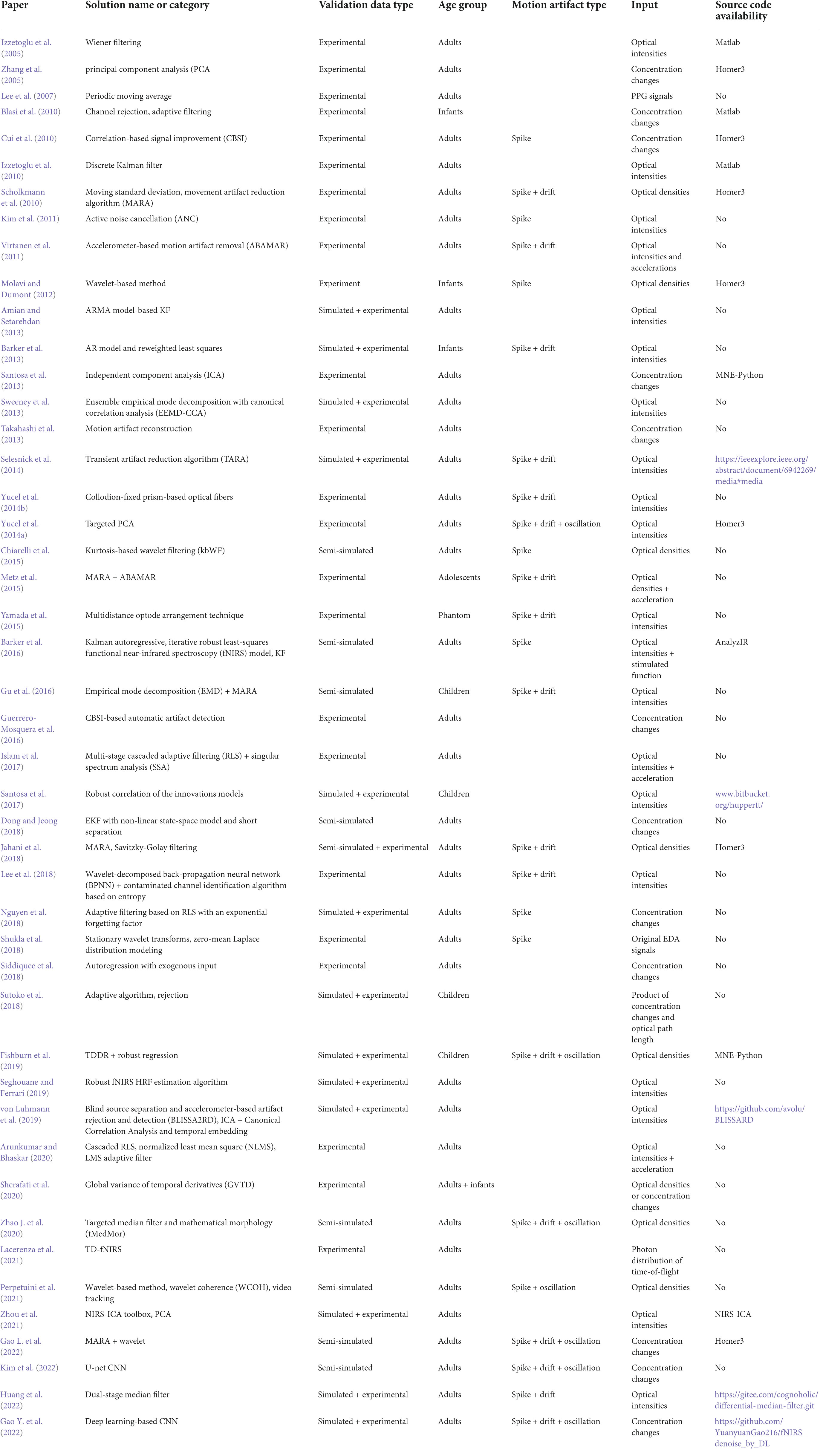
Table 5. List of motion artifact (MA) removal approaches and their relationship.

Comparisons have been made among the trial rejection method, recursive least squares adaptive filtering method (Park et al., 2020), wavelet-based method, ICA, two- or multi-channel regression method, Kalman filter, MARA, PCA, moving average, band-pass filter, median filter, Savitzky–Golay filter, and CBSI for adults’ fNIRS data. Overall, the MA correction approach is better than the trial rejection approach (Brigadoi et al., 2014). MA correction can also help to improve classification accuracy (Janani and Sasikala, 2017). Wavelet-based method, ICA, multiple-channel regression, and MARA had a good performance in noise suppression. When processing children’s fNIRS signals, researchers compared PCA, MARA, wavelet-based method, moving average, CBSI, and tPCA. MARA, tPCA, and CBSI can retain a higher number of trials. The tPCA and MARA are more robust. Moving average, wavelet-based method, and tPCA have a better performance than other methods. Researchers also examined the filtering performance of infants’ fNIRS data. Trial rejection, wavelet-based method, tPCA, MARA, and different processing pipelines were compared in their studies. MA correction can retain many trials, but hemodynamic response functions were also suppressed. The optimal pre-processing pipeline depends on the dataset (Gemignani and Gervain, 2021). Similar to the conclusion for adults’ data, MA correction is better than trial rejection. The wavelet-based method alone or in a stack with MARA and the wavelet-based method (iqr = 0.5) had better performance in noise suppression. MARA in a stack with the wavelet-based method can recover a higher number of trials.

Reportedly, the wavelet-based filter has good performance when MAs are caused by sudden large movements (or spikes). Moreover, ICA and multi-channel regression also perform well in terms of noise suppression (Robertson et al., 2010). Cooper et al. (2012) reported that PCA, MARA, wavelet-based method, Kalman filter, and trial rejection method could reduce the MSE in corrupted fNIRS signals (Cooper et al., 2012). PCA, MARA, and wavelet-based methods exhibited much better performance than the other methods (Piper et al., 2014). In contrast, Brigadoi et al. (2014) claimed that the Kalman filter performed better using the area under the curve (AUC ratio) of the mean hemodynamic responses than PCA, and MARA, followed by the wavelet-based method and CBSI. They also claimed that the wavelet-based method exhibited a better performance in reducing the AUC for the first two seconds after stimulus onset (AUC_0–2).

Therefore, the evaluation of MA removal techniques depends on the evaluation metrics of the researchers. Due to this phenomenon, multiple metrics need to be considered when comparing various methods. Cooper et al. (2012) used MSE to assess how different solutions can suppress MAs and contrast-to-noise ratio (CNR) to evaluate how well the solutions can retain brain activation signals. Janani and Sasikala (2017) reported that a band-pass filter, median filter, and Savitzky-Golay filter could increase the CNR. Additionally, the performance of the MA solutions differs from each other when the MA types are different. Figure 5 showed an example of MA removal using different filters.

FIGURE 5

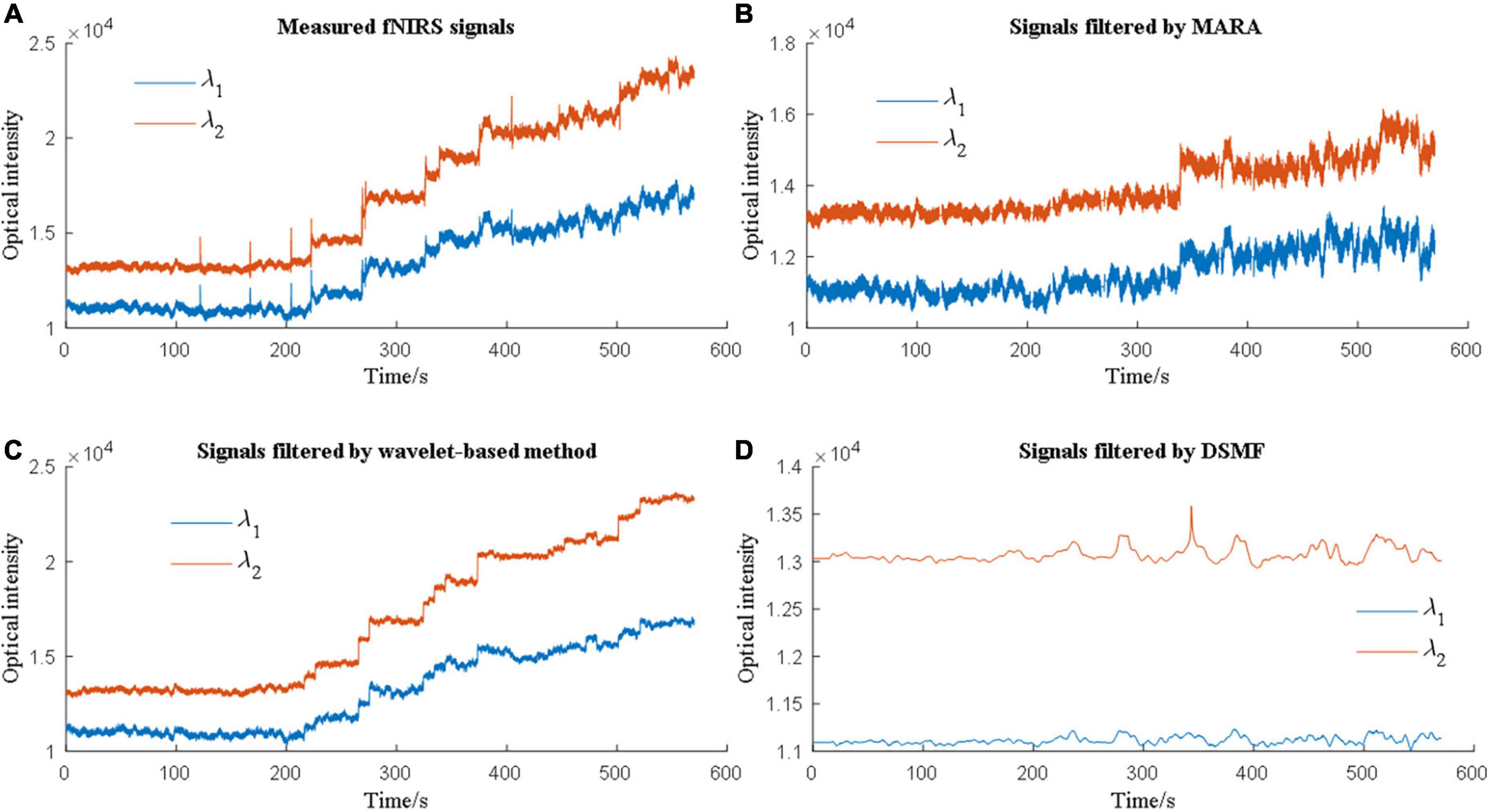
Figure 5. Different motion artifact (MA) removal techniques have different performances when processing experimental data.

The optimal solution for different age groups can be different. Hu et al. (2015) tested the MA removal performance of six solutions using fNIRS data from children: wavelet-based method, PCA, MARA, moving average, CBSI, and the combination of moving average and wavelet-based methods. It was found that MARA successfully suppressed all types of MAs but had an unsatisfactory AUC ratio. Moving average and wavelet-based method turned out to be better solutions for children. Meanwhile, CBSI was efficient in removing spike-like and fast step-like MAs. Besides, Reyes et al. (2018) claimed that tPCA was the best solution for processing children’s fNIRS signals and the authors added that CBSI occasionally produced unstable hemodynamic responses. However, the authors also claimed that MARA was robust and performed well in both AUC and the average standard deviation of each trial-specific hemodynamic response. The contradiction between Reyes and Hu’s findings regarding the MARA originates from improper artifact correction (Hu et al., 2015). Another study by Di Lorenzo et al. (2019) used a combination of MARA and wavelet-based methods and found it to be more effective for infant data than using trial rejection, MARA, or wavelet alone. They further justified that using MA correction could retain many trials. Similar results were obtained by Behrendt et al. (2018). They claimed that trial rejection was not recommended for infants’ data. Table 6 summarizes the data type, age group, techniques in comparison, and main conclusions of all nine comparison papers.

TABLE 6

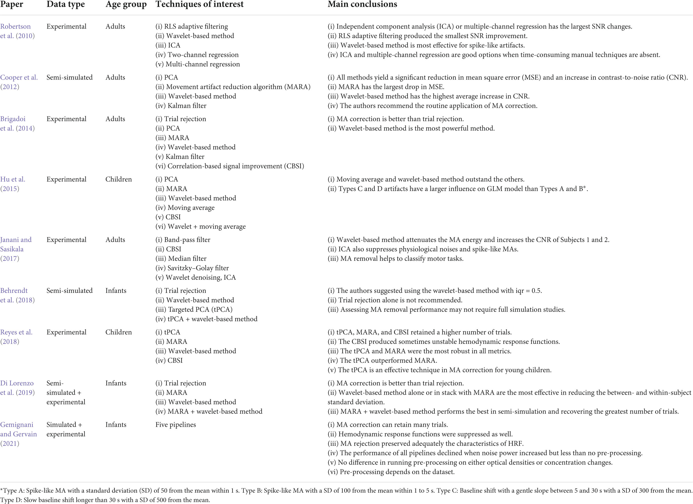
Table 6. Data type, age group, motion artifact (MA) removal techniques and main conclusions in the studies of MA comparison.

Evaluation metrics

Various evaluation metrics have been defined in the literature for noise suppression and signal distortion to quantitatively evaluate the performance of artifact removal solutions. Some metrics have been defined to describe the extent to which the solutions could suppress the artifacts, while others were designed to assess the signal distortion after data processing. In this section, we introduce the details of several metrics for artifact removal except for some commonly used metrics such as root-mean-squared error (to assess the square-root distance between filtered signals and reference signals), the area under the curves (AUC. e.g., researchers can take the initial 1–2 s and the 2–6 s of HbO concentrations) (Reyes et al., 2018), and the t-test (e.g., used together with GLM) (Hu et al., 2015).

Noise suppression

Signal to noise ratio

The signal-to-noise ratio (ΔSNR) in motion artifact removal (Izzetoglu et al., 2005) is different from the more commonly known signal-to-noise ratio (SNR), which is simply the ratio between the power of real signals and the power of noises expressed in decibel. ΔSNR (ΔSNR) is defined as the difference between the estimation SNR (SNR_e) and the input SNR (SNR_i). The two variables are defined as follows.

$SN{R}_e=10{\text{log}}_{10}\left(\frac{\text{Var}\left(x\right)}{\text{Var}\left(\widehat{x}-x\right)}\right)(87)$

$SN{R}_i=10{\text{log}}_{10}\left(\frac{\text{Var}\left(x\right)}{\text{Var}\left(z-x\right)}\right)(88)$

The operator Var(⋅) denotes the variance of the variable in the parentheses. A hat over the motionless fNIRS signal x denotes the estimated motionless fNIRS signal, and z denotes the measured fNIRS signal. Subsequently, ΔSNR is defined as follows.

$\mathrm{\Delta }SNR=SN{R}_e-SN{R}_i(89)$

If the filter of interest can perfectly remove motion artifacts in z, then ΔSNR→ + ∞. If ΔSNR < 0, the filter of interest amplifies the artifacts in the measured signal. Otherwise, the filter can partially remove motion artifacts. In contrast, the larger the ΔSNR, the better the performance of the filter. Physically, the metric describes how well the filter can attenuate motion artifacts in the measured signals.

Since a motionless fNIRS signal is required in the calculation, ΔSNR can be well suited to evaluate the filtering performance of the simulated data. When applied to experimental data, a desired motionless signal is required in place of the motionless fNIRS signal.

Contrast to noise ratio

The contrast to noise ratio (CNR) describes the difference in the fNIRS signal before and during stimulation (Zhang et al., 2005). Here, the subscript “pre” denotes any signal before the stimulus, and the subscript “dur” denotes any signal during the stimulus. The CNR can then be computed as follows.

$CNR=\frac{{\overline{\widehat{x}}}_{\text{dur}}-{\overline{\widehat{x}}}_{\text{pre}}}{\sqrt{{\mathrm{\sigma }}_{\text{dur}}^2+{\mathrm{\sigma }}_{\text{pre}}^2}+ϵ}(90)$

where σ_dur and σ_pre denote the standard deviations of the filtered fNIRS signals during and before the stimulus, and ϵ corresponds to a small non-negative constant compensating for channels with a small stimulus response but relatively low activity. Empirically, ∈= 0.1 μM. In some studies, ∈ was ignored. When MAs exist, the CNR map may appear as all active or negative channels. The active and inactive areas spread throughout the map. Once MAs are properly removed, CNR maps with more concise active zones can be obtained (Kohno et al., 2007).

Percent root difference

The percent root difference (PRD) is a metric that describes how well the two signals match each other (Scholkmann et al., 2010; Dong and Jeong, 2018). When using the motionless signal x as a reference, the PRD is defined as follows.

$PRD=\mathrm{100\%}\times \sqrt{\sum _{i=1}^N\frac{{\left(\widehat{x}\left(i\right)-x\left(i\right)\right)}^2}{{\sum }_{i=1}^N{x}^2\left(i\right)}}(91)$

The smaller the PRD, the better the filtered signals match the motionless signals, that is, fewer artifacts exist in the filtered signals.

Artifact power attenuation

Artifact power attenuation (APA) indicates how much the artifacts in the measured signal can be suppressed in the signal of interest within the corrupted segments (Molavi and Dumont, 2012). Therefore, the metric is expressed in decibels as follows.

$APA=10{\log }_{10}\frac{{\sum }_{i\in A_m}{\left(z^{\text{HP}}\left(i\right)\right)}^2}{{\sum }_{i\in A_m}{\left({\widehat{x}}^{\text{HP}}\left(i\right)\right)}^2}(92)$

where A_m denotes the set of time segments in which the MAs occur. The set constrains the evaluation domain within corrupted segments. The superscript HP denotes a high-pass signal. It is introduced to remove low-frequency physiological variants (Molavi and Dumont, 2012). Since the measured signals are placed in the nominator, the larger the APA, the better the filter of interest that can suppress MAs. Typically, APA is expressed in decibels (Shukla et al., 2018).

APA can directly reveal a filter’s resistance to MAs without disturbance from physiological noise. When using APA, the high-pass filter needs to be chosen carefully to ensure efficient filtering of the physiological noise. Importantly, the filters for both the nominator and denominator should be identical to facilitate a fair comparison.

Within/between-subject standard deviation

Within-subject standard deviation and between-subject standard deviation are two different metrics for evaluating the performance of the MA filter on the experimental data. Within-subject standard deviation refers to the average standard deviation of single-trial hemodynamic responses for a given channel and chromophore. N_trl denotes the number of trials in the signals, k denotes the sample index, i denotes the trial index, and N denotes the number of samples in a trial. Δ$\widehat{c}$_i(k) is the estimated concentration change at instance k in trial i.

${\mathrm{\sigma }}_{\text{within}}=\frac{{\sum }_{k=1}^N{\text{std}}_i\left(\mathrm{\Delta }{\widehat{c}}_i\left(k\right)\right)}{N},i=1,\text{…}\mathrm{ },N_{\text{trl}}(93)$

In practice, there is a within-subject standard deviation for each chromophore in each channel of each subject. The metric is used under the assumption that most of the variability between single-trial hemodynamic responses for each subject is because of the influence of MAs. When comparing the two signals, the within-subject standard deviations can be computed for each chromophore, channel, and subject. Then, the two values were mapped to a point in a scatter plot. We can compare the filtering performance of the two filters by counting the number of points below or above the line y = x.

The between-subject standard deviation refers to the standard deviation of the averaged hemodynamic responses across subjects for each channel (Brigadoi et al., 2014; Di Lorenzo et al., 2019). N_sub denotes the number of subjects, i denotes the subject number, N denotes the number of samples in an experiment, and Δ$\widehat{c}$_i(k) denotes the estimated concentration change at instant k of subject i. The between-subject standard deviation becomes

${\mathrm{\sigma }}_{\text{between}}=\frac{{\sum }_{k=1}^{N_{\text{sub}}}{\text{std}}_i\left(\mathrm{\Delta }{\widehat{c}}_i\left(k\right)\right)}{N},i=1,\text{…}\mathrm{ },N_{\text{sub}}(94)$

It is assumed that the MAs dominate the variability of hemodynamic responses across subjects when using the metric.

Signal distortion

Correlation coefficient

There are two methods for evaluating the motion artifact removal performance using the correlation coefficient. The first method computes the correlation between a reference signal and a block-average signal (Zhang et al., 2005). The reference signal was obtained by shifting the rectangular pulse signal to the right. The desired metric is then calculated as the correlation coefficient between the reference signal and the block-averaged response of the filtered signal.

The second method defines the difference in the correlation coefficient (ΔCC) (Izzetoglu et al., 2005; Jahani et al., 2018) as the difference between the estimated correlation coefficient and the input correlation coefficient, that is,

$\mathrm{\Delta }CC=\text{corr}(x,\widehat{x})-\text{corr}(x,z-x)(95)$

The operator corr(⋅, ⋅) represents the correlation between two variables in brackets. The second term in this definition tends to be zero. If ΔCC < 0, then the filter of interest significantly distorts the motionless signal. As ΔCC is closer to one, the distortion reduces in the filtered signal.

Similar to ΔSNR, ΔCC is well-suited for simulated data. When applied to experimental data, reference motionless signals are required in place of motionless fNIRS signals. In contrast, the first definition of the correlation metric requires an experimental paradigm, primarily because it compares the shifted rectangular pulse signal and the block-averaged response.

Pearson product-moment correlation coefficient

This metric appeared in 2008 and was designed to measure the similarity between two signals (Scholkmann et al., 2010). The coefficient is defined as follows.

$r=\frac{1}{M}\sum _{i=1}^N\left(\frac{\widehat{x}\left(i\right)-\overline{\widehat{x}}\left(i\right)}{{\mathrm{\sigma }}_{\widehat{x}}}\right)\left(\frac{x\left(i\right)-\overline{x}\left(i\right)}{{\mathrm{\sigma }}_x}\right)(96)$

where σ denotes the standard deviation and M = N–1. Moreover, the coefficient can also be used to evaluate the similarity between the motionless signal x and measured signal z. The only difference is the replacement of the estimated motionless signal with z in the equation. It is used to calculate the improvement of the proposed method compared with the measurement. The more significant the absolute difference between r($\widehat{x}$, x) and r(x, z), the better the performance of the proposed method. As r becomes closer to one, there is less distortion in the signal of interest. Occasionally, the difference in the Pearson product-moment correlation coefficient can also be used to evaluate the improvement of the filtered signals. The difference is defined as follows.

$\mathrm{\Delta }r=r(\widehat{x},x)-r(z,x)(97)$

The difference may be expressed as a percentage.

Data type compatibility

According to Table 5, three types of data exist: (i) Simulated data, (ii) semi-simulated data, and (iii) experimental data. A semi-simulated dataset can be generated by adding desired concentration changes to MA-corrupted experimental data at resting state, or by adding uncorrupted experimental data at the resting state to the sum of desired concentration changes and designed artifact sequence. For both simulated and semi-simulated datasets, the ground-truth motionless signals are known. Nevertheless, this is not true for experimental datasets. Therefore, the input requirements of each metric decide the metric’s compatible data types. Table 7 summarizes the data type compatibility of different metrics.

TABLE 7

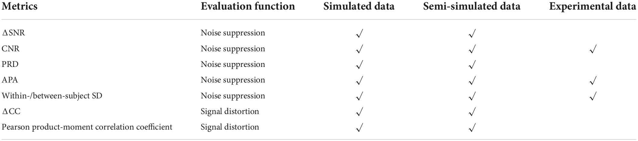
Table 7. Suitability checking of the defined metrics to three types of data.

Conclusion and outlook

This review suggests that removing MAs is unavoidable in developing a more generalized fNIRS device. Literature reported that fNIRS demonstrate a good tolerance to motion artifacts when well-positioned (Pinti et al., 2020). However, a generalized fNIRS apparatus may not guarantee that all users will stick to this rule. The introduction of motion artifact removal techniques will add to the device’s robustness and stability even when the users are involved in significant physical activities. These improvements will add to a positive user experience. The MA issue will become crucial for portable and wearable fNIRS devices. Once the problem is solved, we can envision a more exciting application of fNIRS to connect people or connect the real world with the digital world. Additionally, Tables 5 and 6 show that the filtering performance of one method on different age group can be divers. Hence, for a specific application, a study regarding the optimal solution is still necessary. Our in-depth review can help experienced researchers as well as novices in three ways. First, a brief introduction to some core solutions from a different perspective can help gain a better understanding as to how the solutions can be replicated, whether they are suitable for online or offline applications, and their advantages and disadvantages. Second, the definitions and physical meanings of commonly used metrics were summarized. Researchers can select the best metrics according to their requirements. Third, a sketch of the latest developments in MA removal techniques can help readers familiarize themselves with the field and decide their research focus. This review can be served as a list of different motion artifact removal solutions. When targeting the application of fNIRS, readers can pick the methods or metrics fulfilling their requirements for their specific scenario. When attacking a better noise removal solution, readers can develop their theory from the methods mentioned in this work or take another path.

The research in MA removal has made significant progress since the early 21st century. Different attempts have been made to remove MAs, especially for offline processing. Some researchers have also investigated the role of MA removal techniques in fNIRS data analysis pipelines (Gemignani and Gervain, 2021). Some studies managed to find out the optimal techniques among several candidates when doing experiments on a targeted population (Hu et al., 2015; Behrendt et al., 2018; Reyes et al., 2018; Di Lorenzo et al., 2019). Some attempted to solve the problem by improving the optical models (Scholkmann et al., 2014b; Yamada et al., 2015).

However, this review also revealed several lacunae concerning MA removal. First, no research has explained how to achieve a balance between the use of auxiliary hardware and that of an algorithmic solution. A comparative study compared an adaptive filter (accelerometer is needed) with wavelet-based filtering, ICA, two-channel, and multi-channel regression (Robertson et al., 2010); however, it is far from sufficient. Second, the existing online MA removal solutions are primarily validated for noise suppression and signal distortion, but their filtering delays are not evaluated. An online solution with high noise suppression, low signal distortion, and low delay is significant for portable and wearable fNIRS devices. Third, the robustness and compatibility of the solutions in different application scenarios were not thoroughly studied. A solution’s filtering performance may change when the user’s age, tasks, external disturbance, or user’s physical health are different. This issue is crucial for developing application-oriented fNIRS devices, such as devices that operate in extreme environments or a targeted population.

The research to remove MAs is not a method-oriented topic but an application-oriented topic. Any solution that can help make one step further to either general applications or a specific application would be advantageous to the fNIRS community.

Author Contributions

RH and K-SH designed the structure and scope of the review. RH aggregated reviewed articles and prepared the first draft manuscript. DY and GH verified the equations. K-SH reviewed and revised the manuscript. All authors contributed to the article and approved the submitted version.

Funding

This work was supported in part by the China Scholarship Council (grant no. 201808260086) and in part by the Technology Innovation Program (grant no. 20016846, Development of fNIRS-based multimonitoring healthcare device for sleep state diagnosis) funded by the Ministry of Trade, Industry & Energy, South Korea.

Conflict of interest

The authors declare that the research was conducted in the absence of any commercial or financial relationships that could be construed as a potential conflict of interest.

The reviewer NN declared a past co-authorship with the author K-SH to the handling editor.

Publisher’s note

All claims expressed in this article are solely those of the authors and do not necessarily represent those of their affiliated organizations, or those of the publisher, the editors and the reviewers. Any product that may be evaluated in this article, or claim that may be made by its manufacturer, is not guaranteed or endorsed by the publisher.

References

Abtahi, M., Amiri, A. M., Byrd, D., and Mankodiya, K. (2017). Hand motion detection in fNIRS neuroimaging data. Healthcare 5:5020020. doi: 10.3390/healthcare5020020

PubMed Abstract | CrossRef Full Text | Google Scholar

Afkhami, R. G., Walker, F. R., Ramadan, S., and Johnson, S. J. (2019). A dynamic model of brain hemodynamics in near-infrared spectroscopy. IEEE Transac. Biomed. Eng. 2019, 1–1. doi: 10.1109/TBME.2019.2954829

PubMed Abstract | CrossRef Full Text | Google Scholar

Akgul, C. B., Sankur, B., and Akin, A. (2005). Spectral analysis of event-related hemodynamic responses in functional near infrared spectroscopy. J. Comput. Neurosci. 18, 67–83. doi: 10.1007/s10827-005-5478-2

PubMed Abstract | CrossRef Full Text | Google Scholar

Amian, M., and Setarehdan, S. K. (2013). Motion artifact reduction in functional near infrared spectroscopy signals by autoregressive moving average modeling based Kalman filtering. J. Innov. Opt. Health Sci. 6:1350035. doi: 10.1142/S1793545813500351

CrossRef Full Text | Google Scholar

Arunkumar, K. R., and Bhaskar, M. (2020). Heart rate estimation from wrist-type photoplethysmography signals during physical exercise. Biomed. Sig. Proc. Cont. 57:101790. doi: 10.1016/j.bspc.2019.101790

CrossRef Full Text | Google Scholar

Balardin, J. B., Morais, G. A. Z., Furucho, R. A., Trambaiolli, L., Vanzella, P., Biazoli, C., et al. (2017). Imaging brain function with functional near-infrared spectroscopy in unconstrained environments. Front. Hum. Neurosci. 11:258. doi: 10.3389/fnhum.2017.00258

PubMed Abstract | CrossRef Full Text | Google Scholar

Barker, J. W., Aarabi, A., and Huppert, T. J. (2013). Autoregressive model based algorithm for correcting motion and serially correlated errors in fNIRS. Biomed. Optics Exp. 4, 1366–1379. doi: 10.1364/BOE.4.001366

PubMed Abstract | CrossRef Full Text | Google Scholar

Barker, J. W., Rosso, A. L., Sparto, P. J., and Huppert, T. J. (2016). Correction of motion artifacts and serial correlations for real-time functional near-infrared spectroscopy. Neurophotonics 3:031410. doi: 10.1117/1.NPh.3.3.031410

CrossRef Full Text | Google Scholar

Bartocci, M., Winberg, J., Ruggiero, C., Bergqvist, L. L., Serra, G., and Lagercrantz, H. (2000). Activation of olfactory cortex in newborn infants after odor stimulation: a functional near-infrared spectroscopy study. Pediat. Res. 48, 18–23. doi: 10.1203/00006450-200007000-00006

PubMed Abstract | CrossRef Full Text | Google Scholar

Behrendt, H. F., Firk, C., Nelson, C. A., and Perdue, K. L. (2018). Motion correction for infant functional near-infrared spectroscopy with an application to live interaction data. Neurophotonics 5, 015004. doi: 10.1117/1.NPh.5.1.015004

CrossRef Full Text | Google Scholar

Blasi, A., Phillips, D., Lloyd-Fox, S., Koh, P. H., and Elwell, C. E. (2010). Automatic detection of motion artifacts in infant functional optical topography studies. Oxy. Transport Tissue 662, 279–284. doi: 10.1007/978-1-4419-1241-1_40

CrossRef Full Text | Google Scholar

Brigadoi, S., Ceccherini, L., Cutini, S., Scarpa, F., Scatturin, P., Selb, J., et al. (2014). Motion artifacts in functional near-infrared spectroscopy: a comparison of motion correction techniques applied to real cognitive data. Neuroimage 85, 181–191. doi: 10.1016/j.neuroimage.2013.04.082

PubMed Abstract | CrossRef Full Text | Google Scholar

Chiarelli, A. M., Maclin, E. L., Fabiani, M., and Gratton, G. (2015). A kurtosis-based wavelet algorithm for motion artifact correction of fNIRS data. Neuroimage 112, 128–137. doi: 10.1016/j.neuroimage.2015.02.057

PubMed Abstract | CrossRef Full Text | Google Scholar

Chiarelli, A. M., Zappasodi, F., Di Pompeo, F., and Merla, A. (2017). Simultaneous functional near-infrared spectroscopy and electroencephalography for monitoring of human brain activity and oxygenation: a review. Neurophotonics 4:041411. doi: 10.1117/1.NPh.4.4.041411

CrossRef Full Text | Google Scholar

Cooper, R. J., Seib, J., Gagnon, L., Phillip, D., Schytz, H. W., Iversen, H. K., et al. (2012). A systematic comparison of motion artifact correction techniques for functional near-infrared spectroscopy. Front. Neurosci. 6:147. doi: 10.3389/fnins.2012.00147

PubMed Abstract | CrossRef Full Text | Google Scholar

Cui, X., Baker, J. M., Liu, N., and Reiss, A. L. (2015). Sensitivity of fNIRS measurement to head motion: an applied use of smartphones in the lab. J. Neurosci. Methods 245, 37–43. doi: 10.1016/j.jneumeth.2015.02.006

PubMed Abstract | CrossRef Full Text | Google Scholar

Cui, X., Bray, S., and Reiss, A. L. (2010). Functional near infrared spectroscopy (NIRS) signal improvement based on negative correlation between oxygenated and deoxygenated hemoglobin dynamics. Neuroimage 49, 3039–3046. doi: 10.1016/j.neuroimage.2009.11.050

PubMed Abstract | CrossRef Full Text | Google Scholar

Di Lorenzo, R., Pirazzoli, L., Blasi, A., Bulgarelli, C., Hakuno, Y., Minagawa, Y., et al. (2019). Recommendations for motion correction of infant fNIRS data applicable to multiple data sets and acquisition systems. Neuroimage 200, 511–527. doi: 10.1016/j.neuroimage.2019.06.056

PubMed Abstract | CrossRef Full Text | Google Scholar

Dong, S., and Jeong, J. (2018). Improvement in recovery of hemodynamic responses by extended Kalman filter with non-linear state-space model and short separation measurement. IEEE Transac. Biomed. Eng. 66, 2152–2162. doi: 10.1109/TBME.2018.2884169

PubMed Abstract | CrossRef Full Text | Google Scholar

Dybvik, H., and Steinert, M. (2021). Real-world fNIRS brain activity measurements during Aashtanga Vinyasa yoga. Brain Sci. 11:742. doi: 10.3390/brainsci11060742

PubMed Abstract | CrossRef Full Text | Google Scholar

Fantini, S., Hueber, D., Franceschini, M. A., Gratton, E., Rosenfeld, W., Stubblefield, P. G., et al. (1999). Non-invasive optical monitoring of the newborn piglet brain using continuous-wave and frequency-domain spectroscopy. Phys. Med. Biol. 44, 1543–1563. doi: 10.1088/0031-9155/44/6/308

CrossRef Full Text | Google Scholar

Fishburn, F. A., Ludlum, R. S., Vaidya, C. J., and Medvedev, A. V. (2019). Temporal derivative distribution repair (TDDR): a motion correction method for fNIRS. Neuroimage 184, 171–179. doi: 10.1016/j.neuroimage.2018.09.025

PubMed Abstract | CrossRef Full Text | Google Scholar

Gao, L., Wei, Y. H., Wang, Y. F., Wang, G., Zhang, Q., Zhang, J. B., et al. (2022). Hybrid motion artifact detection and correction approach for functional near-infrared spectroscopy measurements. J. Biomed. Optics 27:025003. doi: 10.1117/1.JBO.27.2.025003

CrossRef Full Text | Google Scholar

Gao, Y., Cavuoto, L., Yan, P., Kruger, U., Schwaitzberg, S., De, S., et al. (2020). A deep learning approach to remove motion artifacts in fNIRS data analysis. Biophotonics Congress: Biomedical Optics 2020 (Translational, Microscopy, OCT, OTS, BRAIN). Washington, DC: Optical Society of America, BM2C, 7.

Google Scholar

Gao, Y., Chao, H., Cavuoto, L., Yan, P., Kruger, U., Norfleet, J., et al. (2022). Deep learning-based motion artifact removal in functional near-infrared spectroscopy. Neurophotonics 9:041406. doi: 10.1117/1.NPh.9.4.041406

CrossRef Full Text | Google Scholar

Gemignani, J., and Gervain, J. (2021). Comparing different pre-processing routines for infant fNIRS data. Dev. Cogn. Neurosci. 48:100943. doi: 10.1016/j.dcn.2021.100943

PubMed Abstract | CrossRef Full Text | Google Scholar

Ghafoor, U., Lee, J. H., Hong, K.-S., Park, S. S., Kim, J., and Yoo, H. R. (2019). Effects of acupuncture therapy on MCI patients using functional near-infrared spectroscopy. Front. Aging Neurosci. 11:237. doi: 10.3389/fnagi.2019.00237

PubMed Abstract | CrossRef Full Text | Google Scholar

Ghafoor, U., Yang, D., and Hong, K.-S. (2021). Neuromodulatory effects of HD-tACS/tDCS on the prefrontal cortex: a resting-state fNIRS-EEG study. IEEE J. Biomed. Health Inform. 2021, 1–12. doi: 10.1109/JBHI.2021.3127080

PubMed Abstract | CrossRef Full Text | Google Scholar

Gu, Y., Han, J. X., Liang, Z. H., Yan, J. Q., Li, Z., and Li, X. L. (2016). Empirical mode decomposition-based motion artifact correction method for functional near-infrared spectroscopy. J. Biomed. Optics 21:15002. doi: 10.1117/1.JBO.21.1.015002

CrossRef Full Text | Google Scholar

Guerrero-Mosquera, C., Borragan, G., and Peigneux, P. (2016). Automatic detection of noisy channels in fNIRS signal based on correlation analysis. J. Neurosci. Methods 271, 128–138. doi: 10.1016/j.jneumeth.2016.07.010

PubMed Abstract | CrossRef Full Text | Google Scholar

Haeussinger, F. B., Dresler, T., Heinzel, S., Schecklmann, M., Fallgatter, A. J., and Ehlis, A. C. (2014). Reconstructing functional near-infrared spectroscopy (fNIRS) signals impaired by extra-cranial confounds: an easy-to-use filter method. Neuroimage 95, 69–79. doi: 10.1016/j.neuroimage.2014.02.035

PubMed Abstract | CrossRef Full Text | Google Scholar

Haghighi, M. S., and Pishkenari, H. N. (2021). Real-time topography and hamaker constant estimation in atomic force microscopy based on adaptive fading extended kalman filter. Internat. J. Cont. Automat. Syst. 19, 2455–2467. doi: 10.1007/s12555-020-0076-7

CrossRef Full Text | Google Scholar

Hong, K.-S., and Zafar, A. (2018). Existence of initial dip for BCI: an illusion or reality. Front. Neurorob. 12:69. doi: 10.3389/fnbot.2018.00069

PubMed Abstract | CrossRef Full Text | Google Scholar

Hu, X. S., Arredondo, M. M., Gomba, M., Confer, N., DaSilva, A. F., Johnson, T. D., et al. (2015). Comparison of motion correction techniques applied to functional near-infrared spectroscopy data from children. J. Biomed. Optics 20:126003. doi: 10.1117/1.Jbo.20.12.126003

CrossRef Full Text | Google Scholar

Hu, X. S., Hong, K.-S., Ge, S. Z. S., and Jeong, M. Y. (2010). Kalman estimator- and general linear model-based on-line brain activation mapping by near-infrared spectroscopy. Biomed. Eng. Online 9:82. doi: 10.1186/1475-925X-9-82

PubMed Abstract | CrossRef Full Text | Google Scholar

Huang, R., and Hong, K.-S. (2021). Multi-channel-based differential pathlength factor estimation for continuous-wave fNIRS. IEEE Access 9, 37386–37396. doi: 10.1109/Access.2021.3063120

CrossRef Full Text | Google Scholar

Huang, R., Qing, K., Yang, D., and Hong, K.-S. (2022). Real-time motion artifact removal using a dual-stage median filter. Biomed. Sig. Proc. Cont. 72:103301. doi: 10.1016/j.bspc.2021.103301

CrossRef Full Text | Google Scholar

Huppert, T. J., Diamond, S. G., Franceschini, M. A., and Boas, D. A. (2009). HomER: a review of time-series analysis methods for near-infrared spectroscopy of the brain. Appl. Optics 48, D280–D298. doi: 10.1364/ao.48.00d280

PubMed Abstract | CrossRef Full Text | Google Scholar

Islam, M. T., Zabir, I., Ahamed, S. T., Yasar, M. T., Shahnaz, C., and Fattah, S. A. (2017). A time-frequency domain approach of heart rate estimation from photoplethysmographic (PPG) signal. Biomed. Sig. Proc. Cont. 36, 146–154. doi: 10.1016/j.bspc.2017.03.020

CrossRef Full Text | Google Scholar

Izzetoglu, M., Chitrapu, P., Bunce, S., and Onaral, B. (2010). Motion artifact cancellation in NIR spectroscopy using discrete Kalman filtering. Biomed. Eng. Online 9:16. doi: 10.1186/1475-925x-9-16

PubMed Abstract | CrossRef Full Text | Google Scholar

Izzetoglu, M., Devaraj, A., Bunce, S., and Onaral, B. (2005). Motion artifact cancellation in NIR spectroscopy using Wiener filtering. IEEE Transac. Biomed. Eng. 52, 934–938. doi: 10.1109/Tbme.2005.845243

PubMed Abstract | CrossRef Full Text | Google Scholar

Jahani, S., Setarehdan, S. K., Boas, D. A., and Yucel, M. A. (2018). Motion artifact detection and correction in functional near-infrared spectroscopy: a new hybrid method based on spline interpolation method and Savitzky-Golay filtering. Neurophotonics 5:015003. doi: 10.1117/1.NPh.5.1.015003

CrossRef Full Text | Google Scholar

Janani, A., and Sasikala, M. (2017). Investigation of different approaches for noise reduction in functional near-infrared spectroscopy signals for brain-computer interface applications. Neur. Comp. Appl. 28, 2889–2903. doi: 10.1007/s00521-017-2961-4

CrossRef Full Text | Google Scholar

Jasdzewski, G., Strangman, G., Wagner, J., Kwong, K. K., Poldrack, R. A., and Boas, D. A. (2003). Differences in the hemodynamic response to event-related motor and visual paradigms as measured by near-infrared spectroscopy. Neuroimage 20, 479–488. doi: 10.1016/S1053-8119(03)00311-2

CrossRef Full Text | Google Scholar

Kameyama, M., Fukuda, M., Uehara, T., and Mikuni, M. (2004). Sex and age dependencies of cerebral blood volume changes during cognitive activation: a multichannel near-infrared spectroscopy study. Neuroimage 22, 1715–1721. doi: 10.1016/j.neuroimage.2004.03.050

PubMed Abstract | CrossRef Full Text | Google Scholar

Khan, H., Naseer, N., Yazidi, A., Eide, P. K., Hassan, H. W., and Mirtaheri, P. (2021). Analysis of human gait using hybrid EEG-fNIRS-based BCI system: a review. Front. Hum. Neurosci. 14:613254. doi: 10.3389/fnhum.2020.613254

PubMed Abstract | CrossRef Full Text | Google Scholar

Khan, M. J., and Hong, K.-S. (2015). Passive BCI based on drowsiness detection: an fNIRS study. Biomed. Optics Exp. 6, 4063–4078. doi: 10.1364/BOE.6.004063

PubMed Abstract | CrossRef Full Text | Google Scholar

Khan, R. A., Naseer, N., Qureshi, N. K., Noori, F. M., Nazeer, H., and Khan, M. U. (2018). fNIRS-based neurorobotic interface for gait rehabilitation. J. Neuroeng. Rehabilit. 15:7. doi: 10.1186/s12984-018-0346-2

PubMed Abstract | CrossRef Full Text | Google Scholar

Kim, C.-K., Lee, S., Koh, D., and Kim, B.-M. (2011). Development of wireless NIRS system with dynamic removal of motion artifacts. Biomed. Eng. Lett. 1, 254–259. doi: 10.1007/s13534-011-0042-7

CrossRef Full Text | Google Scholar

Kim, M., Lee, S., Dan, I., and Tak, S. (2022). A deep convolutional neural network for estimating hemodynamic response function with reduction of motion artifacts in fNIRS. J. Neur. Eng. 19:016017. doi: 10.1088/1741-2552/ac4bfc

PubMed Abstract | CrossRef Full Text | Google Scholar

Kohno, S., Miyai, I., Seiyama, A., Oda, I., Ishikawa, A., Tsuneishi, S., et al. (2007). Removal of the skin blood flow artifact in functional near-infrared spectroscopic imaging data through independent component analysis. J. Biomed. Opt. 12:062111. doi: 10.1117/1.2814249

CrossRef Full Text | Google Scholar

Lacerenza, M., Spinelli, L., Buttafava, M., Dalla Mora, A., Zappa, F., Pifferi, A., et al. (2021). Monitoring the motor cortex hemodynamic response function in freely moving walking subjects: a time-domain fNIRS pilot study. Neurophotonics 8:015006. doi: 10.1117/1.NPh.8.1.015006

CrossRef Full Text | Google Scholar

Lee, G., Jin, S. H., and An, J. (2018). Motion artifact correction of multi-measured functional near-infrared spectroscopy signals based on signal reconstruction using an artificial neural network. Sensors 18:2957. doi: 10.3390/s18092957

PubMed Abstract | CrossRef Full Text | Google Scholar

Lee, H. W., Lee, J. W., Jung, W. G., and Lee, G. K. (2007). The periodic moving average filter for removing motion artifacts from PPG signals. Internat. J. Cont. Automat. Syst. 5, 701–706.

Google Scholar

Lee, S. H., Hur, S. W., Kwak, Y. Y., Nam, Y. H., and Kim, C. J. (2021). Ahead-time approach to carrot-chasing guidance law for an accurate trajectory-tracking control. Internat. J. Cont. Automat. Syst. 19, 2634–2651. doi: 10.1007/s12555-020-0413-x

CrossRef Full Text | Google Scholar

Li, B. A., Tan, Y. H., Zhou, L., and Dong, R. L. (2021). Robust-nonsmooth Kalman filtering for stochastic sandwich systems with dead-zone. Internat. J. Cont. Automat. Syst. 19, 101–111. doi: 10.1007/s12555-019-1027-z

CrossRef Full Text | Google Scholar

Li, L., Zhang, H., Nguyen, Q., and Hong, K.-S. (2021). Adaptive parameter identification for nonlinear sandwich systems with hysteresis nonlinearity based guaranteed performance. Internat. J. Cont. Automat. Syst. 19, 942–952. doi: 10.1007/s12555-019-2020-2

CrossRef Full Text | Google Scholar

Lv, X., Fang, Y., Mao, Z., Jiang, B., and Qi, R. (2021). Fault detection for a class of closed-loop hypersonic vehicle system via hypothesis test method. Internat. J. Cont. Automat. Syst. 19, 350–362. doi: 10.1007/s12555-019-0906-7

CrossRef Full Text | Google Scholar

Metz, A. J., Wolf, M., Achermann, P., and Scholkmann, F. (2015). A new approach for automatic removal of movement artifacts in near-infrared spectroscopy time series by means of acceleration data. Algorithms 8, 1052–1075. doi: 10.3390/a8041052

CrossRef Full Text | Google Scholar

Molavi, B., and Dumont, G. A. (2012). Wavelet-based motion artifact removal for functional near-infrared spectroscopy. Physiolog. Meas. 33, 259–270. doi: 10.1088/0967-3334/33/2/259

CrossRef Full Text | Google Scholar

Moosmann, M., Ritter, P., Krastel, I., Brink, A., Thees, S., Blankenburg, F., et al. (2003). Correlates of alpha rhythm in functional magnetic resonance imaging and near infrared spectroscopy. Neuroimage 20, 145–158. doi: 10.1016/s1053-8119(03)00344-6

CrossRef Full Text | Google Scholar

Naseer, N., and Hong, K.-S. (2015). fNIRS-based brain-computer interfaces: a review. Front. Hum. Neurosci. 9:3. doi: 10.3389/fnhum.2015.00003

PubMed Abstract | CrossRef Full Text | Google Scholar

Nguyen, H. D., and Hong, K.-S. (2016). Bundled-optode implementation for 3D imaging in functional near-infrared spectroscopy. Biomed. Opt. Exp. 7, 3491–3507. doi: 10.1364/BOE.7.003491

PubMed Abstract | CrossRef Full Text | Google Scholar

Nguyen, H. D., Yoo, S. H., Bhutta, M. R., and Hong, K.-S. (2018). Adaptive filtering of physiological noises in fNIRS data. Biomed. Eng. Online 17:180. doi: 10.1186/s12938-018-0613-2

PubMed Abstract | CrossRef Full Text | Google Scholar

Nishiyori, R. (2016). fNIRS: an emergent method to document functional cortical activity during infant movements. Front. Psychol. 7:533. doi: 10.3389/fpsyg.2016.00533

PubMed Abstract | CrossRef Full Text | Google Scholar

Novi, S., Roberts, E., Spagnuolo, D., Spilsbury, B., Price, D. M., Imbalzano, C., et al. (2020). Functional near-infrared spectroscopy for speech protocols: characterization of motion artifacts and guidelines for improving data analysis. Neurophotonics 7:015001. doi: 10.1117/1.NPh.7.1.015001

CrossRef Full Text | Google Scholar

Orihuela-Espina, F., Leff, D. R., James, D. R. C., Darzi, A. W., and Yang, G. Z. (2010). Quality control and assurance in functional near infrared spectroscopy (fNIRS) experimentation. Phys. Med. Biol. 55, 3701–3724. doi: 10.1088/0031-9155/55/13/009

CrossRef Full Text | Google Scholar

Park, B., Pham, P., and Hong, K.-S. (2020). Model reference robust adaptive control of control element drive mechanism in a nuclear power plant. Internat. J. Cont. Automat. Syst. 18, 1651–1661. doi: 10.1007/s12555-019-0987-3

CrossRef Full Text | Google Scholar

Perpetuini, D., Cardone, D., Filippini, C., Chiarelli, A. M., and Merla, A. (2021). A motion artifact correction procedure for fNIRS signals based on wavelet transform and infrared thermography video tracking. Sensors 21, 5117. doi: 10.3390/s21155117

PubMed Abstract | CrossRef Full Text | Google Scholar

Pham, P., Kim, G., Nguyen, Q., and Hong, K.-S. (2021). Control of a non-uniform flexible beam: identification of first two modes. Internat. J. Cont. Automat. Syst. 19, 3698–3707. doi: 10.1007/s12555-020-0913-8

CrossRef Full Text | Google Scholar

Pinti, P., Aichelburg, C., Lind, F., Power, S., Swingler, E., Merla, A., et al. (2015). Using fiberless, wearable fNIRS to monitor brain activity in real-world cognitive tasks. Jove-J. Vis. Exp. 2015:e53336. doi: 10.3791/53336

PubMed Abstract | CrossRef Full Text | Google Scholar

Pinti, P., Tachtsidis, I., Hamilton, A., Hirsch, J., Aichelburg, C., Gilbert, S., et al. (2020). The present and future use of functional near-infrared spectroscopy (fNIRS) for cognitive neuroscience. Ann. N Y Acad. Sci. 1464, 5–29.

Google Scholar

Piper, S. K., Krueger, A., Koch, S. P., Mehnert, J., Habermehl, C., Steinbrink, J., et al. (2014). A wearable multi-channel fNIRS system for brain imaging in freely moving subjects. Neuroimage 85, 64–71. doi: 10.1016/j.neuroimage.2013.06.062

PubMed Abstract | CrossRef Full Text | Google Scholar

Radhakrishnan, H., Vanduffel, W., Deng, H. P., Ekstrom, L., Boas, D. A., and Franceschini, M. A. (2009). Fast optical signal not detected in awake behaving monkeys. NeuroImage 45, 410–419. doi: 10.1016/j.neuroimage.2008.12.014

PubMed Abstract | CrossRef Full Text | Google Scholar

Rea, M., Rana, M., Lugato, N., Terekhin, P., Gizzi, L., Brotz, D., et al. (2014). Lower limb movement preparation in chronic stroke: a pilot study toward an fNIRS-BCI for gait rehabilitation. Neurorehabilit. Neur. Rep. 28, 564–575. doi: 10.1177/1545968313520410

PubMed Abstract | CrossRef Full Text | Google Scholar

Reyes, L. M. D., Bohache, K., Wijeakumar, S., and Spencer, J. P. (2018). Evaluating motion processing algorithms for use with functional near-infrared spectroscopy data from young children. Neurophotonics 5:025008. doi: 10.1117/1.NPh.5.2.025008

CrossRef Full Text | Google Scholar

Robertson, F. C., Douglas, T. S., and Meintjes, E. M. (2010). Motion artifact removal for functional near infrared spectroscopy: a comparison of methods. IEEE Transac. Biomed. Eng. 57, 1377–1387. doi: 10.1109/TBME.2009.2038667

PubMed Abstract | CrossRef Full Text | Google Scholar

Safaie, J., Grebe, R., Moghaddam, H. A., and Wallois, F. (2013). Toward a fully integrated wireless wearable EEG-NIRS bimodal acquisition system. J. Neur. Eng. 10:056001. doi: 10.1088/1741-2560/10/5/056001

CrossRef Full Text | Google Scholar

Santosa, H., Aarabi, A., Perlman, S. B., and Huppert, T. J. (2017). Characterization and correction of the false-discovery rates in resting state connectivity using functional near-infrared spectroscopy. J. Biomed. Opt. 22:055002. doi: 10.1117/1.Jbo.22.5.055002

CrossRef Full Text | Google Scholar

Santosa, H., Hong, M. J., Kim, S. P., and Hong, K.-S. (2013). Noise reduction in functional near-infrared spectroscopy signals by independent component analysis. Rev. Sci. Instrum. 84:073106. doi: 10.1063/1.4812785

CrossRef Full Text | Google Scholar

Scholkmann, F., Kleiser, S., Metz, A. J., Zimmermann, R., Pavia, J. M., Wolf, U., et al. (2014a). A review on continuous wave functional near-infrared spectroscopy and imaging instrumentation and methodology. Neuroimage 85, 6–27. doi: 10.1016/j.neuroimage.2013.05.004

PubMed Abstract | CrossRef Full Text | Google Scholar

Scholkmann, F., Metz, A. J., and Wolf, M. (2014b). Measuring tissue hemodynamics and oxygenation by continuous-wave functional near-infrared spectroscopy-how robust are the different calculation methods against movement artifacts? Physiolog. Meas. 35, 717–734. doi: 10.1088/0967-3334/35/4/717

CrossRef Full Text | Google Scholar

Scholkmann, F., Spichtig, S., Muehlemann, T., and Wolf, M. (2010). How to detect and reduce movement artifacts in near-infrared imaging using moving standard deviation and spline interpolation. Physiol. Meas. 31, 649–662. doi: 10.1088/0967-3334/31/5/004

CrossRef Full Text | Google Scholar

Schroeter, M. L., Zysset, S., Kruggel, F., and von Cramon, D. Y. (2003). Age dependency of the hemodynamic response as measured by functional near-infrared spectroscopy. Neuroimage 19, 555–564. doi: 10.1016/S1053-8119(03)00155-1

CrossRef Full Text | Google Scholar

Seghouane, A., and Ferrari, D. (2019). Robust hemodynamic response function estimation from fNIRS signals. IEEE Transac. Sign. Proc. 67, 1838–1848. doi: 10.1109/Tsp.2019.2899289

CrossRef Full Text | Google Scholar

Selb, J., Yucel, M. A., Phillip, D., Schytz, H. W., Iversen, H. K., Vangel, M., et al. (2015). Effect of motion artifacts and their correction on near-infrared spectroscopy oscillation data: a study in healthy subjects and stroke patients. J. Biomed. Opt. 20:056011. doi: 10.1117/1.Jbo.20.5.056011

CrossRef Full Text | Google Scholar

Selesnick, I. W., Graber, H. L., Ding, Y., Zhang, T., and Barbour, R. L. (2014). Transient artifact reduction algorithm (TARA) based on sparse optimization. IEEE Transac. Sign. Proc. 62, 6596–6611. doi: 10.1109/Tsp.2014.2366716

CrossRef Full Text | Google Scholar

Sherafati, A., Snyder, A. Z., Eggebrecht, A. T., Bergonzi, K. M., Burns-Yocum, T. M., Lugar, H. M., et al. (2020). Global motion detection and censoring in high-density diffuse optical tomography. Hum. Brain Mapp. 41, 4093–4112. doi: 10.1002/hbm.25111

PubMed Abstract | CrossRef Full Text | Google Scholar

Shukla, J., Barreda-Angeles, M., Oliver, J., and Puig, D. (2018). Efficient wavelet-based artifact removal for electrodermal activity in real-world applications. Biomed. Sign. Proc. Contr. 42, 45–52. doi: 10.1016/j.bspc.2018.01.009

CrossRef Full Text | Google Scholar

Siddiquee, M. R., Hasan, S. M. S., Marquez, J. S., Ramon, R. N., and Bai, O. (2020). Accurate vigilance detection during gait by using movement artifact removal. IEEE Access 8, 51179–51188. doi: 10.1109/Access.2020.2980546

CrossRef Full Text | Google Scholar

Siddiquee, M. R., Marquez, J. S., Atri, R., Ramon, R., Mayrand, R. P., and Bai, O. (2018). Movement artefact removal from NIRS signal using multi-channel IMU data. Biomed. Eng. Online 17:120. doi: 10.1186/s12938-018-0554-9

PubMed Abstract | CrossRef Full Text | Google Scholar

Sun, Y. B., and Zhao, Y. G. (2021). Distributed cubature kalman filter with performance comparison for large-scale power systems. Internat. J. Cont. Automat. Syst. 19, 1319–1327. doi: 10.1007/s12555-019-1054-9

CrossRef Full Text | Google Scholar

Sutoko, S., Monden, Y., Funane, T., Tokuda, T., Katura, T., Sato, H., et al. (2018). Adaptive algorithm utilizing acceptance rate for eliminating noisy epochs in block-design functional near-infrared spectroscopy data: application to study in attention deficit/hyperactivity disorder children. Neurophotonics 5:045001. doi: 10.1117/1.NPh.5.4.045001

CrossRef Full Text | Google Scholar

Sweeney, K. T., McLoone, S. F., and Ward, T. E. (2013). The use of ensemble empirical mode decomposition with canonical correlation analysis as a novel artifact removal technique. IEEE Transac. Biomed. Eng. 60, 97–105. doi: 10.1109/Tbme.2012.2225427

PubMed Abstract | CrossRef Full Text | Google Scholar

Tak, S., and Ye, J. C. (2014). Statistical analysis of fNIRS data: A comprehensive review. Neuroimage 85, 72–91. doi: 10.1016/j.neuroimage.2013.06.016

PubMed Abstract | CrossRef Full Text | Google Scholar

Takahashi, K., Tanaka, T., Nara, H., Kaneko, S., Inoue, M., Shimizu, S., et al. (2013). A modeling of cerebral blood flow changes due to head motion for fNIRS. Internat. J. Optomechatr. 7, 83–95. doi: 10.1080/15599612.2013.777493

CrossRef Full Text | Google Scholar

Tang, M., Chen, Z., and Yin, F. (2020). Robot tracking in SLAM with Masreliez-Martin unscented Kalman filter. Internat. J. Contr. Automat. Syst. 18, 2315–2325. doi: 10.1007/s12555-019-0669-1

CrossRef Full Text | Google Scholar

Vinette, S. A., Dunn, J. F., Slone, E., and Federico, P. (2015). Artifact reduction in long-term monitoring of cerebral hemodynamics using near-infrared spectroscopy. Neurophotonics 2:025004. doi: 10.1117/1.NPh.2.2.025004

CrossRef Full Text | Google Scholar

Virtanen, J., Noponen, T., Kotilahti, K., Virtanen, J., and Ilmoniemi, R. J. (2011). Accelerometer-based method for correcting signal baseline changes caused by motion artifacts in medical near-infrared spectroscopy. J. Biomed. Opt. 16:087005. doi: 10.1117/1.3606576

CrossRef Full Text | Google Scholar

Vitorio, R., Stuart, S., Rochester, L., Alcock, L., and Pantall, A. (2017). fNIRS response during walking - artefact or cortical activity? a systematic review. Neurosci. Biobehav. Rev. 83, 160–172. doi: 10.1016/j.neubiorev.2017.10.002

PubMed Abstract | CrossRef Full Text | Google Scholar

von Luhmann, A., Boukouvalas, Z., Muller, K. R., and Adali, T. (2019). A new blind source separation framework for signal analysis and artifact rejection in functional near-infrared spectroscopy. Neuroimage 200, 72–88. doi: 10.1016/j.neuroimage.2019.06.021

PubMed Abstract | CrossRef Full Text | Google Scholar

Wan, E. A., and Nelson, A. T. (2001). “Dual extended Kalman filter methods,” in Kalman Filtering and Neural Networks, ed. S. HAYKIN (Hoboken, NJ: John Wiley & Sons, Inc).

Google Scholar

Wei, Y., Wang, Y., Wang, G., and Yan, X. (2018). “Dual-threshold wavelet filtering based motion artifact removal for near-infrared spectroscopy long-term measurement,” in Proceedings of the BIBE 2018; International Conference on Biological Information and Biomedical Engineering, 6–8 June 2018, Shanghai, 1–5.

Google Scholar

Wilcox, T., Bortfeld, H., Woods, R., Wruck, E., and Boas, D. A. (2005). Using near-infrared spectroscopy to assess neural activation during object processing in infants. J. Biomed. Optics 10:011010. doi: 10.1117/1.1852551

CrossRef Full Text | Google Scholar

Wyser, D., Lambercy, O., Scholkmann, F., Wolf, M., and Gassert, R. (2017). Wearable and modular functional near-infrared spectroscopy instrument with multidistance measurements at four wavelengths. Neurophotonics 4:041413. doi: 10.1117/1.NPh.4.4.041413

CrossRef Full Text | Google Scholar

Yamada, T., Umeyama, S., and Ohashi, M. (2015). Removal of motion artifacts originating from optode fluctuations during functional near-infrared spectroscopy measurements. Biomed. Optics Exp. 6, 4632–4649. doi: 10.1364/BOE.6.004632

PubMed Abstract | CrossRef Full Text | Google Scholar

Yang, B., Jia, X. C., and Yang, F. W. (2021). Variational bayesian adaptive unscented kalman filter for RSSI-based indoor localization. Internat. J. Contr. Automat. Syst. 19, 1183–1193. doi: 10.1007/s12555-019-0973-9

CrossRef Full Text | Google Scholar

Yucel, M. A., Selb, J., Cooper, R. J., and Boas, D. A. (2014a). Targeted principle component analysis: a new motion artifact correction approach for near-infrared spectroscopy. J. Innov. Opt. Health Sci. 7:1350066. doi: 10.1142/S1793545813500661

PubMed Abstract | CrossRef Full Text | Google Scholar

Yucel, M. A., Selb, J., Boas, D. A., Cash, S. S., and Cooper, R. J. (2014b). Reducing motion artifacts for long-term clinical NIRS monitoring using collodion-fixed prism-based optical fibers. Neuroimage 85, 192–201. doi: 10.1016/j.neuroimage.2013.06.054

PubMed Abstract | CrossRef Full Text | Google Scholar

Zafar, A., and Hong, K.-S. (2017). Detection and classification of three-class initial dips from prefrontal cortex. Biomed. Opt. Exp. 8, 367–383. doi: 10.1364/BOE.8.000367

PubMed Abstract | CrossRef Full Text | Google Scholar

Zhang, Y. H., Brooks, D. H., Franceschini, M. A., and Boas, D. A. (2005). Eigenvector-based spatial filtering for reduction of physiological interference in diffuse optical imaging. J. Biomed. Opt. 10:011014. doi: 10.1117/1.1852552

CrossRef Full Text | Google Scholar

Zhao, H. B., Brigadoi, S., Chitnis, D., De Vita, E., Castellaro, M., Powell, S., et al. (2020). A wide field-of-view, modular, high-density diffuse optical tomography system for minimally constrained three-dimensional functional neuroimaging. Biomed. Opt. Exp. 11, 4110–4129. doi: 10.1364/BOE.394914

PubMed Abstract | CrossRef Full Text | Google Scholar

Zhao, J., Qiao, J. R. M. T., Ding, X. T., and Liang, X. M. (2020). fNIRS signal motion correction algorithm based on mathematical morphology and median filter. ACTA Optica Sinica 40:2230002. doi: 10.3788/Aos202040.2230002

CrossRef Full Text | Google Scholar

Zhao, H. B., and Cooper, R. J. (2018). Review of recent progress toward a fiberless, whole-scalp diffuse optical tomography system. Neurophotonics 5:011012. doi: 10.1117/1.NPh.5.1.011012

CrossRef Full Text | Google Scholar

Zhao, H. B., Frijia, E. M., Rosas, E. V., Collins-Jones, L., Smith, G., Nixon-Hill, R., et al. (2021). Design and validation of a mechanically flexible and ultra-lightweight high-density diffuse optical tomography system for functional neuroimaging of newborns. Neurophotonics 8:015011. doi: 10.1117/1.NPh.8.1.015011

CrossRef Full Text | Google Scholar

Zhao, Y., Sun, P. P., Tan, F. L., Hou, X., and Zhu, C. Z. (2021). NIRS-ICA: A Matlab toolbox for independent component analysis applied in fNIRS studies. Front. Neuroinform. 15:683735. doi: 10.3389/fninf.2021.683735

PubMed Abstract | CrossRef Full Text | Google Scholar

Zhou, L. F., Chen, C., Liu, Z. H., Hu, Y. Y., Chen, M. Y., Li, Y. F., et al. (2021). A coarse/fine dual-stage motion artifacts removal algorithm for wearable NIRS systems. IEEE Sens. J. 21, 13574–13583. doi: 10.1109/Jsen.2021.3069553

CrossRef Full Text | Google Scholar

Zhou, Z. B., Wu, J., Li, Y., Fu, C., and Fourati, H. (2017). Critical issues on kalman filter with colored and correlated system noises. Asian J. Cont. 19, 1905–1919. doi: 10.1002/asjc.1545

CrossRef Full Text | Google Scholar