Prior Compensation Algorithm for Cerenkov Luminescence Tomography From Single-View Measurements

Cerenkov luminescence tomography (CLT) has attracted much attention because of the wide clinically-used probes and three-dimensional (3D) quantification ability. However, due to the serious morbidity of 3D optical imaging, the reconstructed images of CLT are not appreciable, especially when single-view measurements are used. Single-view CLT improves the efficiency of data acquisition. It is much consistent with the actual imaging environment of using commercial imaging system, but bringing the problem that the reconstructed results will be closer to the animal surface on the side where the single-view image is collected. To avoid this problem to the greatest extent possible, we proposed a prior compensation algorithm for CLT reconstruction based on depth calibration strategy. This method takes full account of the fact that the attenuation of light in the tissue will depend heavily on the depth of the light source as well as the distance between the light source and the detection plane. Based on this consideration, a depth calibration matrix was designed to calibrate the attenuation between the surface light flux and the density of the internal light source. The feature of the algorithm was that the depth calibration matrix directly acts on the system matrix of CLT reconstruction, rather than modifying the regularization penalty items. The validity and effectiveness of the proposed algorithm were evaluated with a numerical simulation and a mouse-based experiment, whose results illustrated that it located the radiation sources accurately by using single-view measurements.

Introduction

Cerenkov luminescence imaging (CLI) provides a potential solution to the problem of clinical translation of optical imaging, because many radionuclide probes that are widely used in clinic can be used as the light emission source of CLI. Since Robertson used a CCD camera to collect the Cerenkov luminescence (CL) from a small animal in 2009, the CLI has been rapidly developed and widely used in the biomedical fields (1–5). However, CLI is a method of two-dimensional (2D) planar imaging, which cannot provide the three-dimensional (3D) spatial distribution of the radionuclide probes. Thus, it cannot accurately quantify and analyze these probes as well as the molecules they target (6). This problem can be solved by its 3D derivatives, namely the Cerenkov luminescence tomography (CLT). CLT reconstructs the spatial distribution of the internal radionuclide probes by integrating the CL images measured from the body surface with the structural information and other prior information (7–13). Li et al. first proposed the concept of CLT, reconstructing the 3D distribution of ¹⁸FDG in a homogeneous mouse model (8). The homogenous model is relatively simple, and is quite different from the real imaging organisms, resulting in inaccurate results. This can be solved by more complex heterogeneous model (8, 9, 11, 14, 15). However, due to the serious morbidity of CLT reconstruction, the quality of the reconstructed images needs to be further improved. There are several ways to reduce the ill-posedness and improve the quality of the reconstruction results, including combining the strategies of permissible source region, multi-view or multispectral measurements, and regularization terms (16–19). These strategies are designed to improve the ill-posedness by reducing the dimension of the domain to be solved, increasing the dimension and number of measurements, or regulating regularization penalties. Increasing the amount of measured data is one of commonly used methods. However, a large amount of reconstruction data undoubtedly increases the reconstruction time and limit the reconstruction efficiency. Using a small amount of data to obtain accurate reconstruction results is an important problem to be solved at this stage.

In the process of image acquisition of CLI, especially when using a commercial system, small animals usually lie flat on the animal holder. In this case, only the CL light emitted from the top surface of the animal can be collected. This leads to the need of 3D reconstruction based on incomplete or single-view images. Single-view based reconstruction can reduce data acquisition time, and can use less data to reconstruct the targeted probes within live organisms (20). However, the reconstructed results based on the single-view image will be closer to the animal surface on the side where the single-view image is collected. For single-view imaging, the light from the point near the surface of the imaging object contributes more to the collected image, whereas the point far away contributes less. This is due to the lack of other views signals, resulting in the detector’s detection sensitivity to points far away from the detection surface becomes weak. Liu proposed a depth compensation algorithm for diffuse optical tomography (DOT) (21–23), which compensates the detection sensitivity loss by constructing depth compensation matrix. However, in the DOT imaging mode, the light source is known and located outside the organism, which is different from the CLT with unknown light source located inside the organism.

Inspired by the depth compensation algorithm in DOT, and considering that the attenuation of light in tissues depends heavily on the depth of light emission source as well as the distance between the light emission source and the detection plane, here we proposed a prior compensation algorithm for CLT reconstruction based on depth calibration strategy. CL image detected from single-view results in the loss of other views of luminescent signals. The farther away from the detection plane, the greater the loss of the luminescent signals can be. Thus, a depth calibration matrix was designed to calibrate the signal loss between the detected surface light flux and the density of internal light source. The depth calibration matrix has the same dimensions as CLT system matrix, and is composed of different compensation weights. Here, the compensation weights are determined using the detection plane as a benchmark, which is where they differ from those in existing studies (21–23). In the calibration process, the larger weight will be given to the points far away from the detection plane, and the smaller weight will be given to the points near. This calibration can balance the detection sensitivity loss in depth direction due to the increase of depth. With the help of this strategy, the inaccuracy of CLT reconstruction from single-view image can be improved. We evaluate the validity and effectiveness of the proposed method with a numerical simulation and a mouse-based experiment.

Methods

When the fluctuation of CL is neglected, the radiative transfer equation (RTE) can be used to accurately describe the propagation process of CL light in medium. However, in the practical application, it is hard to imagine the calculation cost of solving RTE directly. Several compromised schemes for RTE have been proposed, such as Monte Carlo computational model based on statistics and the approximate models based on numerical simplification. Among these approximate models, the diffusion equation (DE), simplified spherical harmonics approximation (SP_N), and their hybrid equation are usually used in 3D optical imaging (24–26). Due to the high accuracy and high computational efficiency in the high diffusion medium, DE has been widely used in the 3D optical imaging of living animals. The expression of the DE is:

$\begin{array}{ll}\{\begin{array}{ll}-\nabla ·\left(D\left(r\right)\nabla \varphi \left(r\right)\right)+{\mu }_a\left(r\right)\varphi \left(r\right)=Q\left(r\right)\hfill & r\in \Omega \hfill \\ J\left(r\right)=-D\left(r\right)\left(v·\nabla \varphi \left(r\right)\right)\hfill & r\in \partial \Omega \hfill \end{array}& (1)\end{array}$

where Ω is the region of interest to be solved, and ∂Ω is its boundary; ø (r) is the nodal flux density at position r;Q (r) denotes the power density of the radionuclide probes; D (r) is the diffusion coefficient that is related to the absorption coefficient and the reduced scattering coefficient; μ_a (r) represents the absorption coefficient; v is the unit outer normal on ∂Ω; and J (r) is the outgoing light flux density measured on the outer boundary.

Through a series of operations, including transforming Eq (1). into weak form, the tetrahedral mesh discretization, and the finite element calculation, Eq (1). can be converted to the following linear equation (27):

$\begin{array}{ll}M\Phi =FQ& (2)\end{array}$

where Q denotes the source matrix, and F is the source weighted matrix; Φ is a nodal flux density related matrix; and M is a sparse positive definite stiffness matrix describing the relationship between the power density of the light source and the measurable nodal flux density. This relationship is determined by the absorption and scattering of tissue, and is highly dependent on the distance between two nodes.

To calibrate the effect of depth on the detection signal, a depth calibration matrix C was designed in this study. The depth calibration matrix has the same dimensions as CLT stiffness matrix, and is composed of different compensation weights. Different from the existing studies (21–23), the compensation weights used in C were determined using the detection plane as a benchmark. In the calibration process, the larger weights will be given to the points far away from the detection plane, and the smaller weights will be given to the points near. After integrating the depth calibration matrix, the matrix equation of Eq (2). can be rewritten as:

$\begin{array}{ll}(MC)\Phi =FQ& (3)\end{array}$

Here, the depth calibration matrix C is defined as:

$\begin{array}{ll}C={[Arr(C^{\#})]}^{\lambda }& (4)\end{array}$

where γ is an adjustable parameter between 0 and 3, determined empirically for practical applications; Arr (•) denotes an operation that rearranges all the elements of a matrix in an order like the original nodes in the M matrix; and C^# is a diagonal matrix with the same dimension as M, and each element is a weighted value determined by the distance between the observed node and the detection plane. This matrix C^# can be determined as follows. Firstly, the matrix M having a dimension of m×m was divided into N submatrix having a dimension of m/N×m. Secondly, the maximum eigenvalue of each submatrix N_k (k=1, 2, …, N) was calculated, and the maximum eigenvalue of the kth submatrix was defined as S_max,k. Thirdly, the average distance of the nodes in each submatrix to the detection plane was calculated, and the submatrices were then renumbered according to these distance values. The submatrix at the tth distance from the detection plane was noted as N_max,t (t=1, 2, …, N). For example, the farthest submatrix from the detection plane was assigned a new number as N_max,1 and the nearest one was N_max,N. Finally, we sorted the N maximum eigenvalues from largest to smallest, and assigned the larger values to the positions of the submatrices with smaller t values. These sorted eigenvalues formed the C^# matrix as the values of the elements on its diagonal. For example, the largest value was assigned to the position in the C^# matrix where the submatrix N_K furthest from the detection plane was located.

Eq (3). can be further converted into the following linear matrix equation between the internal radionuclide source and the boundary measurement:

$\begin{array}{ll}J=AQ& (5)\end{array}$

where J is the exiting light flux current measured at boundary; and$A={[{(MC)}^{–1}F]}_{\Theta }$ with ${[•]}_{\Theta }$ representing an operation of removing the elements in the specified matrix that corresponds to the light flux density at the internal nodes.

Equation (6) is the system matrix of the proposed algorithm for single-view CLT. Since the radionuclide probes are sparse distributed in the animal body and the single-view measurement is seriously insufficient, the solution to Eq (6). can be converted into solving the following sparse regularization problem:

$\begin{array}{ll}Q=\arg \min \frac{1}{2}{\left|\right|AQ-J\left|\right|}_2^2+\mu {\left|Q\right|}_1& (6)\end{array}$

where μ is the regularization parameter, and can be determined empirically in the experiments. In this work, the primal-dual interior-point algorithm was selected to solve Eq (7) (28). In the reconstruction, the initial position of source node was guessed at the center of the solving domain, which was used to construct the depth calibration matrix C.

Experiments and Results

Two groups of experiments, including a numerical simulation and a mouse-based in vivo experiment were conducted to validate the performance of the proposed method. Two indicators were selected to quantitatively evaluate the reconstructed results. The first indicator is the distance error (Dis_Err) that defines the distance between the central position of reconstructed source and the actual center of the radionuclide probe. The second indicator is the depth error (Dep_Err) which is defined as the depth of the reconstructed source minus the depth of the actual radionuclide probe. This depth is relative to the detection plane of the single-view image, that is, the distance from the source to the detection plane is defined as the depth. Moreover, in order to evaluate the superiority of the proposed method, the DE method without depth calibration is selected as a reference for comparison.

Numerical Simulation

In the numerical simulation, to show the advantages of the proposed method in depth reconstruction intuitively, a cube having a side length of 10 cm was selected as the simulation model. The absorption coefficient of the cube is 0.08 mm^-1, and the reduced scattering coefficient is 10 mm^-1. A sphere having a radius of 5 mm was employed as the light source, acting as the radionuclide probes. In order to investigate the performance of the depth compensation method, we placed the light source at different depths of 1 cm, 3 cm, and 5 cm from the detection surface respectively. Figure 1 shows the diagram of the simulation model (Figure 1A) and the depth definition (Figure 1B). The measured image on the detected surface was obtained by solving the SP₃ equation on the highly dense grid with the finite element method. The cube model was divided into 103,545 tetrahedrons and 18,471 nodes to form the highly dense grid. Single-view image from one of the planes of the cube was used as the measurements for reconstruction. In the process of the inverse reconstruction, the finite element discretization is completely different from that used in the forward simulation. The reconstruction was performed on a coarse mesh that consists of 18,262 tetrahedrons and 3,495 nodes. Finally, the proposed algorithm-based reconstruction method and the traditional DE method without combining the prior compensation algorithm were performed to locate the distribution of the mimic radioactive tracer.

FIGURE 1

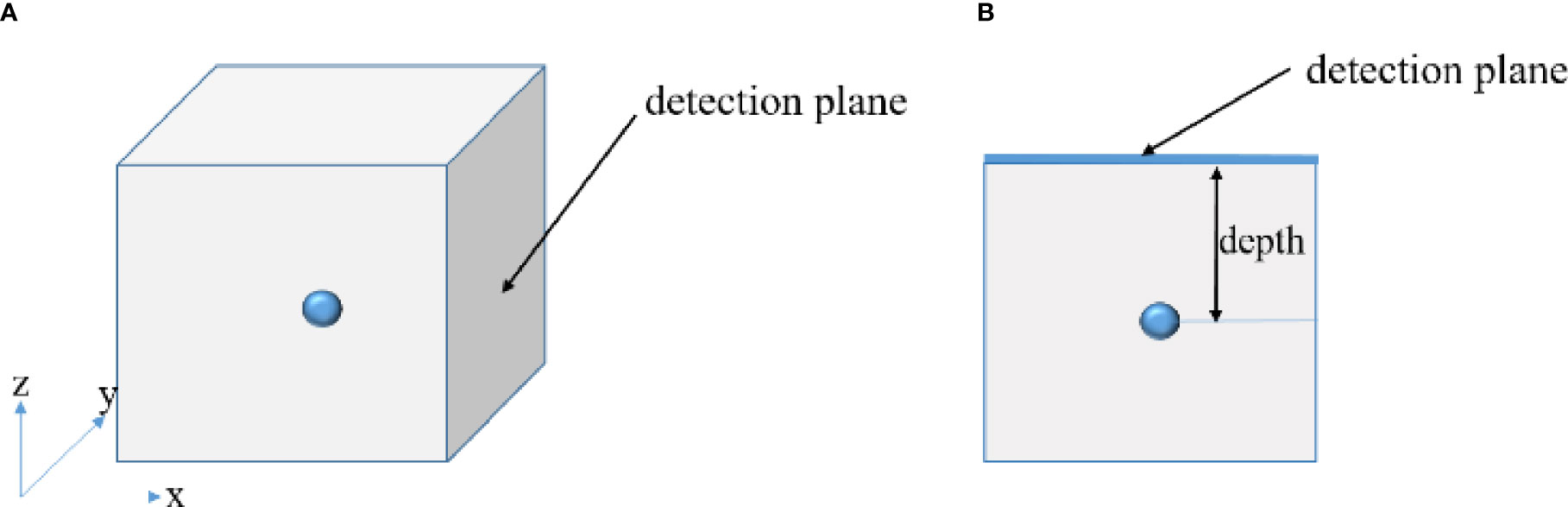
Figure 1 Schematic diagrams of the simulation model indicating where the single-view image was collected (A) and of the definition of the depth (B).

Figure 2 shows the comparison results reconstructed by the proposed and reference methods. Therein, Figures 2A–C show the 3D reconstruction results of the reference method with the light source at depth of 1 cm, 3 cm and 5 cm respectively, and Figures 2D–F present the corresponding results of the prior compensation algorithm-based method. The blue solid spheres mark the actual distribution of the mimic radioactive tracer, and the colored tetrahedrons are the reconstructed source. First of all, we can find that when the depth of the light source was 1 cm, both the prior compensation algorithm-based method and the reference method can locate the distribution of the light source relatively accurately. This means that the attenuation of the signal transmission to the detection plane is not significant when the light source is located at shallow depths. However, as the depth of the light source increases, the attenuation of the signal transmission to the detection plane starts to become significant and can affect the results of the CLT reconstruction. For example, when the depth increased to 3 cm and 5 cm, the reference method cannot locate the light source well, and the reconstructed results tend to the surface on the side of the detection plane. Moreover, almost all the reconstructed tetrahedrons were outside the sphere where the actual light source was. On the contrary, the proposed algorithm can still locate the position of the light source accurately, and all the reconstructed tetrahedrons were concentrated inside the sphere where the light source was. These results confirmed that the a priori compensation algorithm is indeed effective for the reconstruction of deep light source and proved the advantages of the proposed method for the single-view reconstruction of deep light source.

FIGURE 2

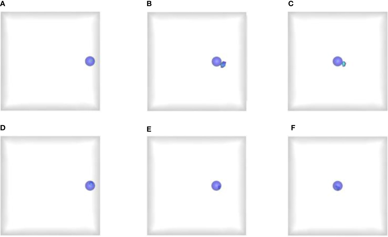
Figure 2 Reconstructed results obtained by the proposed and reference methods. (A–C) The reconstructed results of the reference method at depth of 1 cm, 3 cm and 5 cm respectively; (D–F) The reconstructed results of the proposed method at depth of 1 cm, 3 cm and 5 cm respectively. The blue solid spheres mark the actual distribution of the mimic radioactive tracer, and the colored tetrahedrons are the reconstructed source.

In order to quantitatively evaluate the reconstruction results, we calculated two indicators of Dis_Err and Dep_Err, as presented in Figure 3. Therein, the black bars show the distance or depth errors of the reconstructed results by the reference method, and the red bars represent those obtained by the proposed method. From these quantitative results, almost the same conclusion was addressed that the proposed method greatly improved the accuracy of the reconstruction results and reduced the depth positioning error, especially for the light sources at deeper depth. With the increase of the depth of the light source, the effect of this improvement became more obvious. For example, for the positioning accuracy of the light sources (Figure 3A), when the depth of the light source was 1 cm, the Dis_Err was similar for both methods, and the improvement ratio of the proposed method compared with the reference method was only 1.18. As the depth increased, the improvement ratio increased further, for example to 2.02 at 3 cm depth and 2.63 at 5 cm depth. For the depth resolving accuracy of the light sources (Figure 3B), a similar trend was obtained with the depth of the light source. As the depth increased from 1 cm to 5 cm, the improvement ratio of the proposed method compared with the reference one increased from 1.89 to 6.6. These quantitative results collectively demonstrated that the depth calibration matrix has a good regulatory effect on the depth of the reconstructed results, and the proposed algorithm can well compensate the inaccuracy of the reconstructed results caused by the data loss in the single-view image-based reconstruction.

FIGURE 3

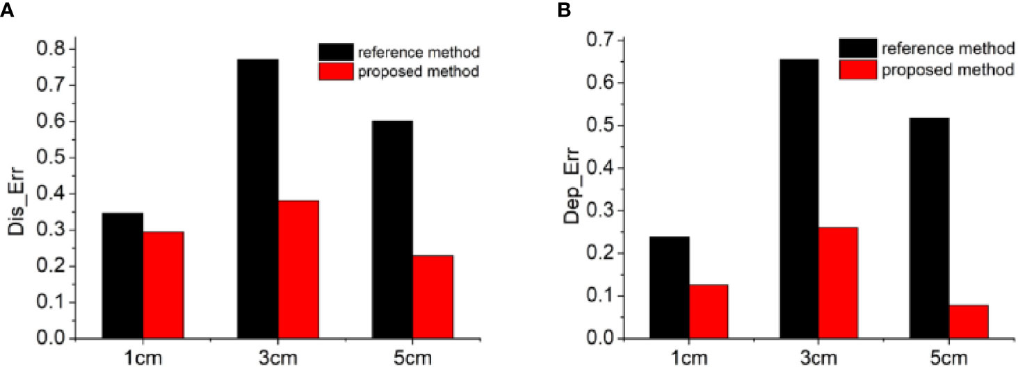
Figure 3 Quantitative analysis of the reconstruction results. The calculated values of the indicators of Dis_err (A) and Dep_err (B). The black bars show the distance or depth errors of the reconstructed results by the reference method, and the red bars represent those obtained by the proposed method.

Mouse Based In Vivo Experiment

After the feasibility and effectiveness of the proposed method were verified with numerical simulation, we carried out a live mouse based in vivo experiment to further prove the application potential. In the experiment, an athymic male nude mouse was used as the imaging model, who is approximately six weeks old. All procedures were performed in accordance with the animal protocol of Xi’an Jiaotong University Animal Care and Use Committee, China (No. XJTULAC2016-412). Firstly, an artificial Cerenkov luminescent source was prepared, which was made of a glass vessel containing about 400 μCi ¹⁸F-FDG. The size of the artificial source was about 1 mm in diameter and 5 mm in length. The artificial source was then implanted into the liver of the living mouse. The mouse was placed on a flat animal platform after anesthesia, and put into the live small animal imaging system (IVIS Kinetic, PerkinElmer) for data collection. By using a filter, a luminescent image at 670 nm was collected on the top surface of the mouse for later reconstruction. The anatomical structural information of the mouse was obtained by our home-made rotating tube μCT system that is comprised of an X-ray tube (Series 5000, Oxford Instruments) and a flat panel detector (C7921CA-02, Hamamatsu). The anatomical structure contained some major organs, such as the lung, liver, heart, kidney, and muscle, their optical properties are listed in Table 1 (29).

TABLE 1

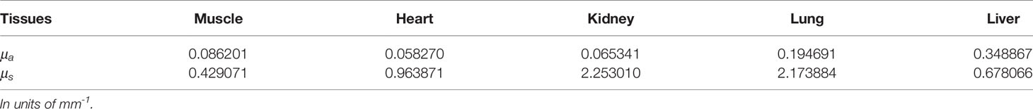
Table 1 Optical parameters of different organs in the mouse model.

Figure 4A shows the anatomical structure of the mouse with the organs highlighted, and these organs were used in the reconstruction. In order to reconstruct the internal light source, the collected single-view image by the CCD camera needs to map onto the mouse surface. Here, the Lambert source theory based energy mapping method was used (30), and the obtained light flux distribution on the mouse surface was shown in Figure 4B. In the reconstruction, the mouse model was discretized into a mesh consisting of 18,235 tetrahedrons and 3,731 nodes. Based on the light flux distribution on the mouse surface and the discretized nodal information, the internal artificial source was reconstructed by the reference and proposed methods respectively, with the results presented in Figures 4C–F. Figures 4C, D show a 3D view of the reconstructed results, which visualises the accurate positioning of the light source. Figures 4E, F give a cross-sectional view of the reconstructed result, such that the reconstructed information on the depth of the light source can be seen in this view. We found that the energy distribution of the light source reconstructed by the proposed method was more concentrated near the actual artificial source (Figure 4D), while the results obtained by the reference method had high energy regions far from the artificial source and close to the body surface towards the detection plane (Figure 4C). Furthermore, quantitative analysis in localization error and depth resolving error were plotted in Figure 4G. From the results presented in Figure 4, we can obtain almost the same conclusion as the numerical simulation. The reconstructed result obtained by the proposed method is greatly improved in both localization and depth resolving ability compared with the traditional DE-based method. In terms of the localization accuracy, the localization error was reduced by 1.9 times by using the proposed method. For the depth resolving ability, the proposed method can improve the depth resolving accuracy by 2.51 times. In particular, the proposed method reconstructed the center of the light source closer to the actual one and overcame the problem that the reconstruction results of the reference method tend to the surface of the object on the side of the detection plane. The reason for the good results was that the proposed method compensated for the loss of the signal emitted from the deep light source to the detection plane. In addition to the advantages in localization and depth resolving accuracy, we also found that the intersection volume between the reconstructed light source and the actual one was larger than that of the reference method. These results are completely consistent with the simulation results, and strongly proved the applicable potential of the proposed method in in vivo living animal imaging.

FIGURE 4

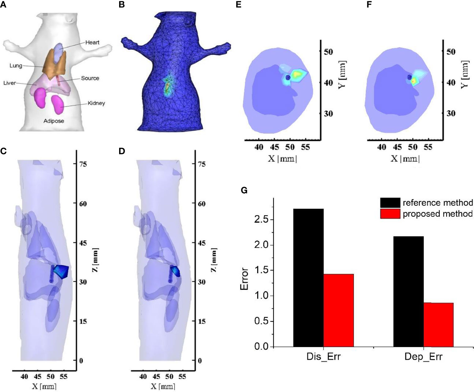
Figure 4 The reconstructed results and related quantitative analysis for the mouse based in vivo experiment. (A) Physical model of the mouse; (B) Light flux distribution on the mouse surface. (C, D) The 3D view of reconstructed images obtained by the reference method and the proposed method respectively; The long blue cylinder is the actual light source obtained by μCT, and the colored tetrahedrons are the reconstructed source; (E, F) The cross-sectional view of reconstructed images obtained by the reference method and the proposed method respectively. (G) The quantitative analysis of these reconstructed results. The black bars represent the quantitative indicators of the reference method, and the red bars are those of the proposed method.

Conclusion

In summary, a prior compensation algorithm was proposed for CLT reconstruction based on depth calibration strategy. This method is more suitable for data acquisition of commercial imaging system, in which a single-view image is often acquired for the reconstruction. Single-view image-based reconstruction will result in the loss of other views of signals. The farther away from the detection plane, the greater the loss of the luminescent signals can be. Thus, the proposed method designed a depth calibration matrix to calibrate the deviation of the depth reconstruction caused by the lack of information. With the help of this strategy, the inaccuracy of CLT reconstruction from single-view image can be improved. The validity and superiority of the prior compensation algorithm were verified using the numerical simulation with the light source at different depths. We also proved the potential of the proposed method in the in vivo applications with the artificial radioactive source based in vivo mouse experiment. There are some shortcomings for current algorithm. For example, in the proposed method, DE is used as the forward model for Cerenkov luminescence transmission, and DE has a limited range of applicability. The next step should incorporate higher order approximation equations or hybrid light propagation models as the forward model. For the construction of the compensation matrix, the center of the light source can be used as the exact starting point for compensation. However, how to determine the light source center also happens to be a problem that needs to be solved for CLT reconstruction, so the exact light source center location is unknown. In the following improvement, the determination of the starting point for compensation can be updated by integrating it into the iterative process of reconstruction. All in all, we believe that the proposed method will further promote the preclinical applications of CLT, especially in large-scale organisms. Our future prospective studies will focus on the biomedical applications of the prior compensation algorithm.

Data Availability Statement

The original contributions presented in the study are included in the article/supplementary material. Further inquiries can be directed to the corresponding author.

Ethics Statement

The animal study was reviewed and approved by Xi’an Jiaotong University Animal Care and Use Committee, China (No. XJTULAC2016-412).

Author Contributions

LW designed the structure and prepared the manuscript. XH and JY modified the manuscript. All authors contributed to the article and approved the submitted version.

Funding

This study was funded by the National Natural Science Foundation of China under Grants 61971350, 62101439, 61901374, 61906154, and 11871321, Natural Science Foundation of Shaanxi under Grants 2019JQ-724, Postdoctoral Innovative Talents Support Program under Grants BX20180254, Scientific and Technological projects of Xi’an under Grant 201805060ZD11CG44, and Education Department Served Local Special Projects under Grant 16JF026.

Conflict of Interest

The authors declare that the research was conducted in the absence of any commercial or financial relationships that could be construed as a potential conflict of interest.

Publisher’s Note

All claims expressed in this article are solely those of the authors and do not necessarily represent those of their affiliated organizations, or those of the publisher, the editors and the reviewers. Any product that may be evaluated in this article, or claim that may be made by its manufacturer, is not guaranteed or endorsed by the publisher.

References

1. Robertson R, Germanos MS, Li C, Mitchell GS, Cherry SR, Silva MD. Optical Imaging of Cerenkov Light Generation From Positron-Emitting Radiotracers. Phys Med Biol (2009) 54(16):N355–65. doi: 10.1088/0031-9155/54/16/N0

PubMed Abstract | CrossRef Full Text | Google Scholar

2. Pogue BW, Feng J, LaRochelle EP, Bruza P, Lin H, Zhang R, et al. Maps of In Vivo Oxygen Pressure With Submillimeter Resolution and Nanomolar Sensitivity Enabled by Cherenkov-Excited Luminescence Scanned Imaging. Nat BioMed Eng (2018) 2:254–64. doi: 10.1038/s41551-018-0220-3

PubMed Abstract | CrossRef Full Text | Google Scholar

3. Cao X, Allu SR, Jiang S, Jia M, Gunn JR, Yao C, et al. Tissue Po2 Distributions in Xenograft Tumors Dynamically Imaged by Cherenkov-Excited Phosphorescence During Fractionated Radiation Therapy. Nat Commun (2020) 11:573. doi: 10.1038/s41467-020-14415-9

PubMed Abstract | CrossRef Full Text | Google Scholar

4. Hu H, Cao X, Kang F, Wang M, Lin Y, Liu M, et al. Feasibility Study of Novel Endoscopic Cerenkov Luminescence Imaging System in Detecting and Quantifying Gastrointestinal Disease: First Human Results. Eur Radiol (2015) 25(6):1814–22. doi: 10.1007/s00330-014-3574-2

PubMed Abstract | CrossRef Full Text | Google Scholar

5. Das S, Haedicke K, Grimm J. Cerenkov-Activated Sticky Tag for In Vivo Fluorescence Imaging. J Nucl Med (2018) 59(1):58–65. doi: 10.2967/jnumed.117.198549

PubMed Abstract | CrossRef Full Text | Google Scholar

6. Dehghani H, Davis SC, Pogue BW. Spectrally Resolved Bioluminescence Tomography Using the Reciprocity Approach. Med Phys (2008) 35(11):4863–71. doi: 10.1118/1.2982138

PubMed Abstract | CrossRef Full Text | Google Scholar

7. Hu Z, Liang J, Yang W, Fan W, Li C, Ma X, et al. Experimental Cerenkov Luminescence Tomography of the Mouse Model With SPECT Imaging Validation. Opt Express (2010) 18(24):24441–50. doi: 10.1364/OE.18.024441

PubMed Abstract | CrossRef Full Text | Google Scholar

8. Li C, Mitchell GS, Cherry SR. Cerenkov Luminescence Tomography for Small-Animal Imaging. Opt Lett (2010) 35(7):1109–11. doi: 10.1364/OL.35.001109

PubMed Abstract | CrossRef Full Text | Google Scholar

9. Zhong J, Tian J, Yang X, Qin C. Whole-Body Cerenkov Luminescence Tomography With the Finite Element SP₃ Method. Ann BioMed Eng (2011) 39(6):1728–35. doi: 10.1007/s10439-011-0261-1

PubMed Abstract | CrossRef Full Text | Google Scholar

10. Gao Y, Ma X, Kang F, Yang W, Liu Y, Wang Z, et al. Enhanced Cerenkov Luminescence Tomography Analysis Based on Y2O3:Eu3+: Rare Earth Oxide Nanoparticles. BioMed Opt Express (2018) 9(12):6091–102. doi: 10.1364/BOE.9.006091

PubMed Abstract | CrossRef Full Text | Google Scholar

11. Wang L, Cao H, Cao X, Ren S, Li K, Zhan Y, et al. Adaptively Hybrid 3rd Simplified Spherical Harmonics With Diffusion Equation-Based Multispectral Cerenkov Luminescence Tomography. IEEE Access (2019) 7(1):160779–85. doi: 10.1109/ACCESS.2019.2950265

CrossRef Full Text | Google Scholar

12. Zhang Z, Cai M, Gao Y, Shi X, Zhang X, Hu Z, et al. A Novel Cerenkov Luminescence Tomography Approach Using Multilayer Fully Connected Neural Network. Phys Med Biol (2019) 64(24):245010. doi: 10.1088/1361-6560/ab5bb4

PubMed Abstract | CrossRef Full Text | Google Scholar

13. Cai MS, Zhang ZY, Shi XJ, Yang JY, Hu ZH, Tian J. Non-Negative Iterative Conves Refinement Approach for Accurate and Robust Reconstruction in Cerenkov Luminescence Tomography. IEEE Trans Med Imaging (2020) 30(10):3207–17. doi: 10.1109/TMI.2020.2987640

CrossRef Full Text | Google Scholar

14. Liu H, Yang X, Song T, Bao C, Shi L, Hu Z, et al. Multispectral Hybrid Cerenkov Luminescence Tomography Based on the Finite Element SP_N Method. J BioMed Opt (2015) 20(8):86007. doi: 10.1117/1.JBO.20.8.086007

PubMed Abstract | CrossRef Full Text | Google Scholar

15. Guo H, He X, Liu M, Zhang Z, Hu Z, Tian J. Weight Multispectral Reconstruction Strategy for Enhanced Reconstruction Accuracy and Stability With Cerenkov Luminescence Tomography. IEEE Trans Med Imaging (2017) 36(6):1337–46. doi: 10.1109/TMI.2017.2658661

PubMed Abstract | CrossRef Full Text | Google Scholar

16. Zhong J, Qin C, Yang X, Chen Z, Yang X, Tian J. Fast-Specific Tomography Imaging via Cerenkov Emission. Mol Imaging Biol (2012) 14(3):286–92. doi: 10.1007/s11307-011-0510-6

PubMed Abstract | CrossRef Full Text | Google Scholar

17. Spinelli AE, Kuo C, Rice BW, Calandrino R, Marzola P, Sbarbati A, et al. Multispectral Cerenkov Luminescence Tomography for Small Animal Optical Imaging. Opt Express (2011) 19(13):12605–18. doi: 10.1364/OE.19.012605

PubMed Abstract | CrossRef Full Text | Google Scholar

18. He X, Liang J, Wang X, Yu J, Qu X, Wang X, et al. Sparse Reconstruction for Quantitative Bioluminescence Tomography Based on the Incomplete Variables Truncated Conjugate Gradient Method. Opt Express (2010) 18(24):24825–41. doi: 10.1364/OE.18.024825

PubMed Abstract | CrossRef Full Text | Google Scholar

19. He X, Yu J, Wang X, Yi H, Chen Y, Song X, et al. Half Thresholding Pursuit Algorithm for Fluorescence Molecular Tomography. IEEE Trans BioMed Eng (2019) 66(5):1468–76. doi: 10.1109/TBME.2018.2874699

PubMed Abstract | CrossRef Full Text | Google Scholar

20. Liu X, Tang X, Shu Y, Zhao L, Liu Y, Zhou T. Single-View Cone-Beam X-Ray Luminescence Optical Tomography Based on Group_YALL1 Method. Phys Med Biol (2019) 64(10):105004. doi: 10.1088/1361-6560/ab1819

PubMed Abstract | CrossRef Full Text | Google Scholar

21. Tian F, Niu H, Khadka S, Lin Z, Liu H. Algorithmic Depth Compensation Improves Quantification and Noise Suppression in Functional Diffuse Optical Tomography. BioMed Opt Express (2010) 1(2):441–52. doi: 10.1364/BOE.1.000441

PubMed Abstract | CrossRef Full Text | Google Scholar

22. Niu H, Tian F, Lin Z, Liu H. Development of a Compensation Algorithm for Accurate Depth Localization in Diffuse Optical Tomography. Opt Lett (2010) 35(3):429–31. doi: 10.1364/OL.35.000429

PubMed Abstract | CrossRef Full Text | Google Scholar

23. Niu H, Lin Z, Tian F, Dhamne S, Liu H. Comprehensive Investigation of Three-Dimensional Diffuse Optical Tomography With Depth Compensation Algorithm. J BioMed Opt (2010) 15(4):046005. doi: 10.1117/1.3462986

PubMed Abstract | CrossRef Full Text | Google Scholar

24. Hu Z, Chen X, Liang J, Qu X, Chen D, Yang W, et al. Single Photon Emission Computed Tomography-Guided Cerenkov Luminescence Tomography. J Appl Phys (2012) 112(2):024703. doi: 10.1063/1.4739266

CrossRef Full Text | Google Scholar

25. Chen Z, Jin X, Li L, Wang G. A Limited-Angle CT Reconstruction Method Based on Anisotropic TV Minimization. Phys Med Biol (2013) 58(7):2119–41. doi: 10.1088/0031-9155/58/7/2119

PubMed Abstract | CrossRef Full Text | Google Scholar

26. Chen X, Sun F, Yang D, Liang J. Coupled Third-Order Simplified Spherical Harmonics and Diffusion Equation-Based Fluorescence Tomographic Imaging of Liver Cancer. J BioMed Opt (2015) 20(9):90502. doi: 10.1117/1.JBO.20.9.090502

CrossRef Full Text | Google Scholar

27. Cong W, Wang G, Kumar D, Liu Y, Jiang M, Wang LV, et al. Practical Reconstruction Method for Bioluminescence Tomography. Opt Express (2005) 13(18):6756–71. doi: 10.1364/opex.13.006756

PubMed Abstract | CrossRef Full Text | Google Scholar

28. Chen X, Yang D, Zhang Q, Liang J. L_1/2 Regularization Based Numerical Method for Effective Reconstruction of Bioluminescence Tomography. J Appl Phys (2014) 115(18):184702. doi: 10.1063/1.4876675

CrossRef Full Text | Google Scholar

29. Alexandrakis G, Rannou FR, Chatziioannou AF. Tomographic Bioluminescence Imaging by Use of a Combined Optical-PET (OPET) System: A Computer Simulation Feasibility Study. Phys Med Biol (2005) 50(17):4225–41. doi: 10.1088/0031-9155/50/17/021

PubMed Abstract | CrossRef Full Text | Google Scholar

30. Chen X, Gao X, Chen D, Ma X, Zhao X, Shen M, et al. 3D Reconstruction of Light Flux Distribution on Arbitrary Surfaces From 2D Multi-Photographic Images. Opt Express (2010) 18(19):19876–93. doi: 10.1364/OE.18.019876

PubMed Abstract | CrossRef Full Text | Google Scholar