Single energy CT-based mass density and relative stopping power estimation for proton therapy using deep learning method

Background: The number of patients undergoing proton therapy has increased in recent years. Current treatment planning systems (TPS) calculate dose maps using three-dimensional (3D) maps of relative stopping power (RSP) and mass density. The patient-specific maps of RSP and mass density were obtained by translating the CT number (HU) acquired using single-energy computed tomography (SECT) with appropriate conversions and coefficients. The proton dose calculation uncertainty of this approach is 2.5%-3.5% plus 1 mm margin. SECT is the major clinical modality for proton therapy treatment planning. It would be intriguing to enhance proton dose calculation accuracy using a deep learning (DL) approach centered on SECT.

Objectives: The purpose of this work is to develop a deep learning method to generate mass density and relative stopping power (RSP) maps based on clinical single-energy CT (SECT) data for proton dose calculation in proton therapy treatment.

Methods: Artificial neural networks (ANN), fully convolutional neural networks (FCNN), and residual neural networks (ResNet) were used to learn the correlation between voxel-specific mass density, RSP, and SECT CT number (HU). A stoichiometric calibration method based on SECT data and an empirical model based on dual-energy CT (DECT) images were chosen as reference models to evaluate the performance of deep learning neural networks. SECT images of a CIRS 062M electron density phantom were used as the training dataset for deep learning models. CIRS anthropomorphic M701 and M702 phantoms were used to test the performance of deep learning models.

Results: For M701, the mean absolute percentage errors (MAPE) of the mass density map by FCNN are 0.39%, 0.92%, 0.68%, 0.92%, and 1.57% on the brain, spinal cord, soft tissue, bone, and lung, respectively, whereas with the SECT stoichiometric method, they are 0.99%, 2.34%, 1.87%, 2.90%, and 12.96%. For RSP maps, the MAPE of FCNN on M701 are 0.85%, 2.32%, 0.75%, 1.22%, and 1.25%, whereas with the SECT reference model, they are 0.95%, 2.61%, 2.08%, 7.74%, and 8.62%.

Conclusion: The results show that deep learning neural networks have the potential to generate accurate voxel-specific material property information, which can be used to improve the accuracy of proton dose calculation.

Advances in knowledge: Deep learning-based frameworks are proposed to estimate material mass density and RSP from SECT with improved accuracy compared with conventional methods.

1 Introduction

The number of patients receiving proton therapy treatment is rising each year. Current proton treatment planning systems (TPS) incorporate relevant proton energy deposition physics into the process, determining the patient irradiation pattern. All patients treated with radiotherapy (including protons) are simulated using computed tomography (CT) typically acquired using a single energy scanning protocol. This data is utilized for geometrical implementation of the therapy and also to characterize the patient from the point of view of the probability of charged particle interactions. Therefore, proton dose calculation accuracy is dependent on the capability of TPS to characterize patient tissues based on CT imaging (1). This is done by correlating the CT number of tissue substitute phantoms with known material composition with mass density or relative stopping power (RSP) via the stoichiometric calibration method (2). The accuracy of this approach relies on the difference between patient tissue chemical composition and the tissue substitute database used in the calibration (3–5). Since single-energy computed tomography (SECT) can’t differentiate changes in CT number as a result of differences in either mass density or material chemical composition (6), the error in RSP calculation can become significant. The accuracy of mass density estimation dominates the uncertainty of RSP (7). Furthermore, tissue heterogeneity, CT image noise, and artifacts can also contribute to the RSP calculation error. The direct consequence of uncertainties associated with material characterization (mass density) from SECT data is a loss of accuracy in the prediction of energy deposition relative to the depth of proton interaction, also called proton range uncertainty. To mitigate range uncertainty, TPS have options to allow for the addition of margins in the proton beam range, the standard being 2.5%-3.5% of the energy-dependent range plus an additional 1mm-1.5mm (8).

To further increase the proton therapy therapeutic ratio advantage, many efforts have been made to decrease the proton range uncertainty. One approach is introducing Monte-Carlo dose calculation algorithms to proton TPS (8–12), which can reduce the margin down to 2.4% plus 1.2 mm (8, 13). Another proposed avenue was to use dual-energy CT (DECT) to build calibration curves between CT number and mass density (14). The methodology allows for the acquisition of CT scans with different X-ray spectra, which in turn can be used to determine relative electron density and mean excitation energy (15). Furthermore, DECT virtual monochromatic image reconstruction techniques can reduce beam hardening artifacts and noise. Numerous algorithms for DECT-based RSP estimation have been developed, and the reported results indicate that the errors in RSP estimates can be reduced to 1% (15–17).

As a robust implementation platform for DECT applications in the area of RSP mapping, machine learning (ML) algorithms have also been applied. Su et al. reported their approach for generating parametric maps using ML, which produced accurate effective atomic numbers, relative electron density, mean excitation energy, and RSP from DECT data (18), and they concluded that artificial neural network (ANN) outperformed other reported ML methods. Building on the potential advantage of increased network depth and compositionality (19, 20), deep learning (DL) is an extension of machine learning, which consists of massive multilayered networks or artificial neurons that can discover useful features in CT images (21). DL methods were successfully applied to improve mass density and RSP mapping from DECT datasets (22).

Despite all DECT-based ML and DL applications for improving proton dose calculation, SECT is still the current standard in clinical CT simulators for proton therapy. Therefore, an accurate and efficient method to reduce range uncertainty based on SECT images would benefit existing proton radiotherapy clinics and workflows. DL networks have high degrees of freedom of modeling, therefore offering the opportunity to improve the accuracy of SECT-based RSP and mass density modeling, as has been shown in DECT-based studies. In this study, we investigate the feasibility of using DL models to correlate SECT-based CT numbers to voxel-specific mass density and RSP using two types of electron density phantoms.

2 Materials and methods

2.1 Phantom SECT data sets

A CIRS 062M electron density phantom (Computerized Imaging Reference Systems, Inc., Norfolk, VA, USA) was used to generate the DL training dataset, while Gammex 467-1009 electron density phantom, CIRS ATOM M701 (male) and M702 (female) anthropomorphic phantoms were chosen to generate the DL networks prediction datasets (Figure 1). Table 1 details the mass density and RSP value for the phantoms used. All mass density information was provided by the manufacturer except the bone insert, for which measurements were utilized to produce a reference value (11). All RSP values were calculated using a previously reported method (22). Phantoms were imaged using a Siemens SOMATOM Definition Edge CT scanner and clinical 120 kVp single energy beam acquisition protocols. The electron density phantom was scanned using a standard head-and-neck protocol. A pelvis protocol was used for the Gammex electron density phantom, while the M701 and M702 phantoms were scanned using three different protocols: head-and-neck (HN), thorax, and pelvis protocols. The manufacturer-reported CTDI_vol is reported in Table 2, as well as the reconstructed image resolution. All the reconstructed SECT images have a reconstructed field-of-view diameter of 500 mm and a slice thickness of 0.5 mm.

FIGURE 1

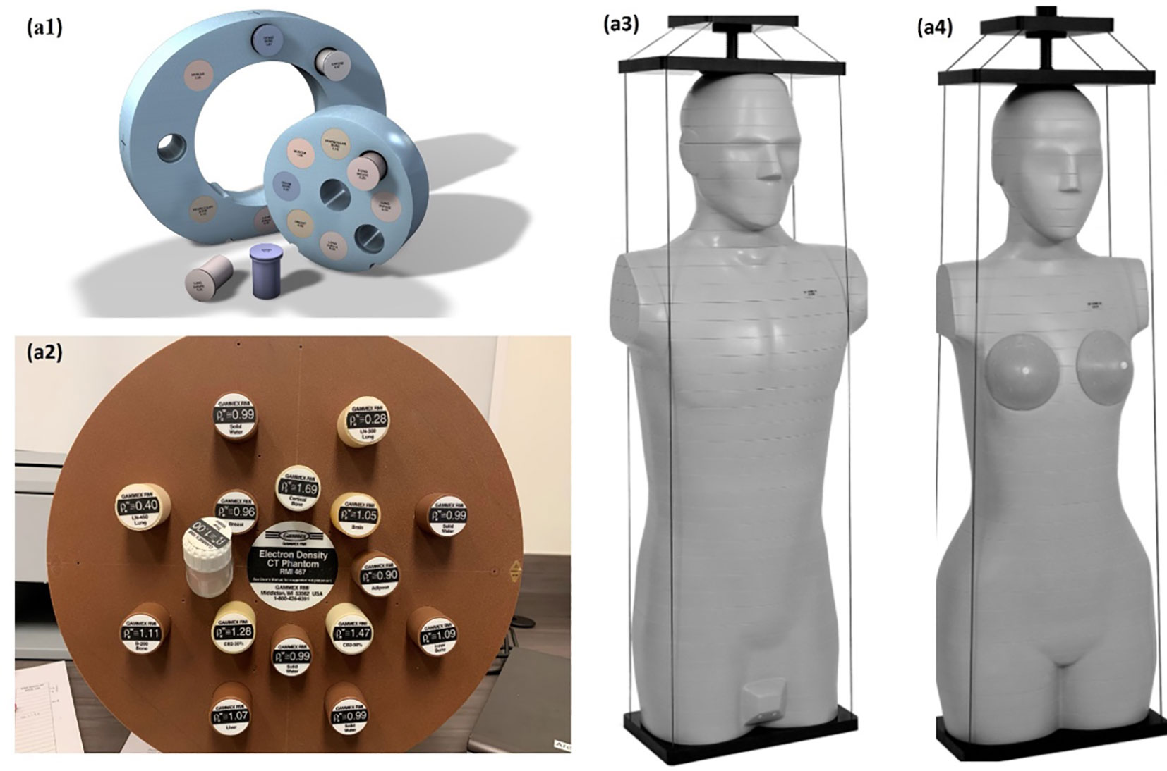
Figure 1 Experiment set up, CIRS 062M electron density phantom (Computerized Imaging Reference Systems) (A1), Gammex 468 electron density phantom (A2) CIRS M701 (A3), and CIRS M702 (Computerized Imaging Reference Systems) (A4) were scanning with Siemens SOMATOM Definition Edge scanner.

TABLE 1

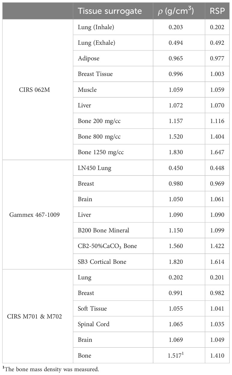
Table 1 Phantom insert data: mass densities and RSP.

TABLE 2

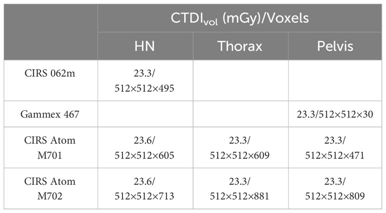
Table 2 CTDI_vol and voxel grid spacing information at each site with specified standard acquisition protocol.

2.2 Deep learning models

Three supervised DL models were implemented to demonstrate the capability of artificial intelligence (AI) to improve proton range calculation using SECT (21, 23–25). Figure 2A shows the artificial neural network (ANN) workflow, and Figures 2B, C show the fully convolutional neural network (FCNN) and residual neural network (ResNet). 120 kVp spectra SECT images are used as DL input. The same DL models are utilized to estimate both the mass density and RSP relative to the input SECT CT number values. The DL models were supervised by a loss function, defined as the difference between the true value and predicted value at each voxel. All the DL models were implemented in PyTorch (26). Su et al. reported that ANN with 30 hidden units outperforms traditional ML models in generating quantitative parametric maps based on DECT images (18). Their ANN design was adopted for SECT parametric mapping in this study, with 30 hidden hyperbolic-tangent (tanh) layers and error backpropagation (see Figure 2A). Convolutional neural networks (CNNs) have gained widespread adoption in both regression and classification tasks over the past decade. This popularity is primarily due to their capability to autonomously learn deep, intricate features, a significant advancement over the traditional machine learning models that relied on manually extracted, handcrafted features (27). A fully connected neural network (FCNN) is a type of CNN that has fully connected hidden layers. A 1D FCNN model was previously implemented to correlate the mass density and RSP map based on DECT parametric maps (22). This 1D FCNN model was adapted to the SECT images dataset input in this study, including seven hidden layers (Figure 2B).

FIGURE 2

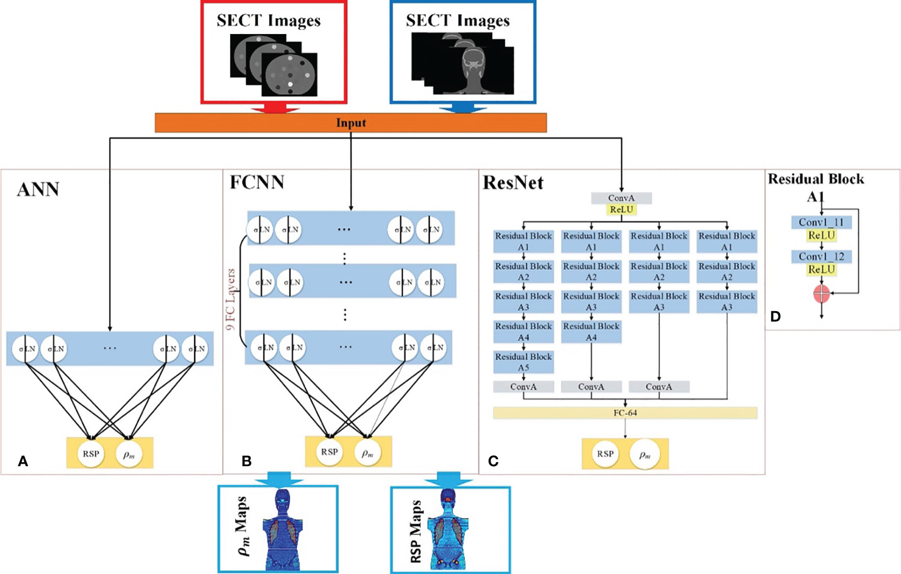
Figure 2 Deep learning framework for mass density and RSP map prediction based on SECT images. The red arrows illustrate the training workflows, while the blue arrows depict the prediction workflow. The framework includes (A) ANN, (B) FCNN, (C) ResNet, and (D) the residual block of ResNet. During the training phase (indicated by red arrows), the phantom SECT images are input into the three deep learning networks: ANN, FCNN, and ResNet. For the prediction phase, the M701 and M702 phantoms are fed into the trained deep learning networks to predict mass density and RSP.

Due to the small size of the training set used in this study, overfitting issues could be associated with trained DL model outputs, which were also considered as vanishing gradient problems for our CNN models. A solution for the latter was proposed: ResNet (25). The ResNet implementation in this study includes a shortcut connection added between input and output after a few weight layers: the residual block. Figure 2C shows the ResNet workflow and Figure 2D shows the detail of the residual block in the ResNet. In Figure 2C, the input is linked to a convolutional layer, which is subsequently connected to four distinct sequences of residual blocks. Each type of residual block varies in terms of channel, kernel, stride, and padding. These details are illustrated in Table 3.

TABLE 3

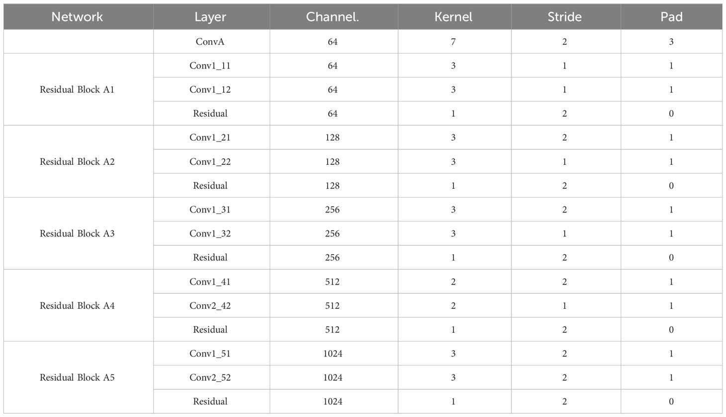
Table 3 Architecture of the 1D convolution components of ResNet (RN).

All the networks were trained using an NVIDIA GeForce 3090 GPU with 24 GB of memory, utilizing a batch size of 100. We set the learning rate for the Adam optimizer to 1e-5. During training, each batch optimization consumed 0.5 GB of CPU memory and 2 GB of GPU memory. All networks were implemented in PyTorch 2.1.

2.3 SECT stoichiometric method

A conventional physics-based SECT stoichiometric calibration method was utilized (2) to provide a standard set of reference values when comparing the DL models output for mass density and RSP. The X-ray linear attenuation coefficient µ of a material can be calculated using Equation (1):

$\begin{array}{ll}\mu =\rho \frac{N_A}{A}[Z{K}^{KN}(E)+Z^n{K}^{SCA}(E)+Z^m{K}^{PE}(E)]& (1)\end{array}$

where $\rho$ is mass density, $N_A$ is Avogadro’s number, A is the atomic weight, Z is the atomic number, $K^{KN}$, $K^{SCA}$, and $K^{PE}$ are weighting constants for incoherent scattering, coherent scattering, and photoelectric effect, respectively, as a function of the SECT scanner X-ray spectrum (1). m and n are constants and were assigned 4.62 and 2.86 (28) for the energies encountered in kV X-ray imaging and the elements present in human tissue. Taking the ratio of the attenuation coefficient of material of interest to the attenuation coefficient of water, equation (2) can be derived:

$\begin{array}{ll}\frac{HU}{1000}+1={\widehat{\rho }}_{e,w}\frac{[1+{\widehat{Z}}^{1.86}{k}_1(E)+{\widehat{Z}}^{3.62}{k}_2(E)]}{[1+{\widehat{Z}}_w{}^{1.86}{k}_1(E)+{\widehat{Z}}_w{}^{3.62}{k}_2(E)]}& (2)\end{array}$

where ${\widehat{\rho }}_{e,w}$ is the electron density relative to water, ${\widehat{Z}}_w$ is the effective atomic number of waters, $k_1=\frac{K^{SCA}}{K^{KN}}$,$k_2=\frac{K^{PE}}{K^{KN}}$. $k_1$ and $k_2$ were calculated by nonlinear regression, while the CT number values were taken as the mean value of each electron density insert from the SECT scan. Finally, the RSP of each material of interest was calculated using the Bethe equation (29):

$\begin{array}{ll}RSP={\widehat{\rho }}_{e,w}\ln [\frac{2m_e{c}^2{\beta }^2}{I_m(1-{\beta }^2)}-{\beta }^2]/\ln [\frac{2m_e{c}^2{\beta }^2}{I_{water}(1-{\beta }^2)}-{\beta }^2]& (3)\end{array}$

where $m_e$ is the electron rest mass, c is the speed of light in vacuum, and β is the proton speed relative to the speed of light. $I_m$ and $I_{water}$ are the mean excitation energies of the material of interest and water. As recommended by ICRU49, $I_{water}$ was set to 75 eV (30). $I_m$ can be calculated from the atomic components using the Bragg additivity rule. Therefore, the stoichiometric calibration method can establish a functional relationship between CT numbers from the SECT datasets and RSP by Equation (2) and (3) (11).

2.4 Empirical model based on DECT parametric mapping

In addition to the stoichiometric calibration standard, a second set of reference values was obtained to compare the DL models output in terms of mass density and RSP prediction based on SECT images against the manufacturer-defined ground truth. These were based on an empirical model for mass density and RSP based on DECT parametric mapping (22), and corresponding definitions are shown in Equation (4) and (5) (7, 31). Therein, $\rho$ denotes the mass density, and ${\rho }_e$ and $Z_{eff}$ are relative electron density and effective atomic number and were obtained from the DECT scanner console (Siemens Healthineers, syngo.via, Malvern, PA, USA). As used, the mass density model has a correction for the inflated lung. The RSP model includes corrections for different human tissues classified by various effective atomic numbers. The same phantoms were used in both DECT and SECT scans, and all tissue surrogate-defined contours were kept the same for reference comparison. Detailed information on DECT scans is listed in a previous publication (22).

$\begin{array}{ll}\rho =\{\begin{array}{c}-0.1746+1.176{\rho }_e \\ 0.26 \end{array}\begin{array}{c}material \ne inflated lung \\ material = inflated lung \end{array}& (4)\end{array}$

$\begin{array}{ll}RSP=\{\begin{array}{c}\begin{array}{c}{\rho }_{e,} \\ (1.1114-0.0148Z_{eff}){\rho }_e\\ 0.9905{\rho }_{e,} \end{array}\\ (1.1117-0.0116Z_{eff}){\rho }_{e,}\end{array}\begin{array}{c} 0\le Z_{eff}<0.5\\ \begin{array}{c}0.5\le Z_{eff}<8.5\\ \begin{array}{c}8.5\le Z_{eff}<10\\ Z_{eff}\ge 10 \end{array}\end{array}\end{array}& (5)\end{array}$

2.5 Evaluation metrics

The ground truth dataset included the reference mass density and RSP values as shown in Table 1. The CIRS M701 and M702 phantom images were manually contoured in RayStation 9B (RaySearch Laboratories, Stockholm, Sweden) for each of the tissue surrogate inserts, and reference values were assigned to each contour. Absolute percentage error (APE) and mean absolute percentage error (MAPE) were calculated as defined in Equation (6) and (7), where i denotes the i^th voxel, x is the mass density or RSP at specific voxel, and N is the total number of voxels. The spatial distribution of error was also generated for the computed APE and displayed in error visualization maps of the whole phantom datasets.

$\begin{array}{ll}AP{E}_i=\left|\frac{x_i-x_{i,REF}}{x_{i,REF}}\right|\times 100\%& (6)\end{array}$

$\begin{array}{ll}MAPE=\frac{1}{N}{\displaystyle {\sum }_{i=1}^{N}AP{E}_i}& (7)\end{array}$

3 Results

3.1 Gammex electron density phantom analysis using pelvis protocol

Table 4 presents results comparing MAPE of mass densities between DL models and the SECT stoichiometric method over seven Gammex electron density phantom tissue surrogates. As emphasized by the bold values, the DL models perform better on all tissue surrogates. For the lung tissue surrogates (LN300 & LN450), the DL models outperform conventional methods, while for higher density inserts, the FCNN and ResNet perform better than the traditional method in select cases. As seen in Table 5, a similar trend can be observed for the DL RSP predictions.

TABLE 4

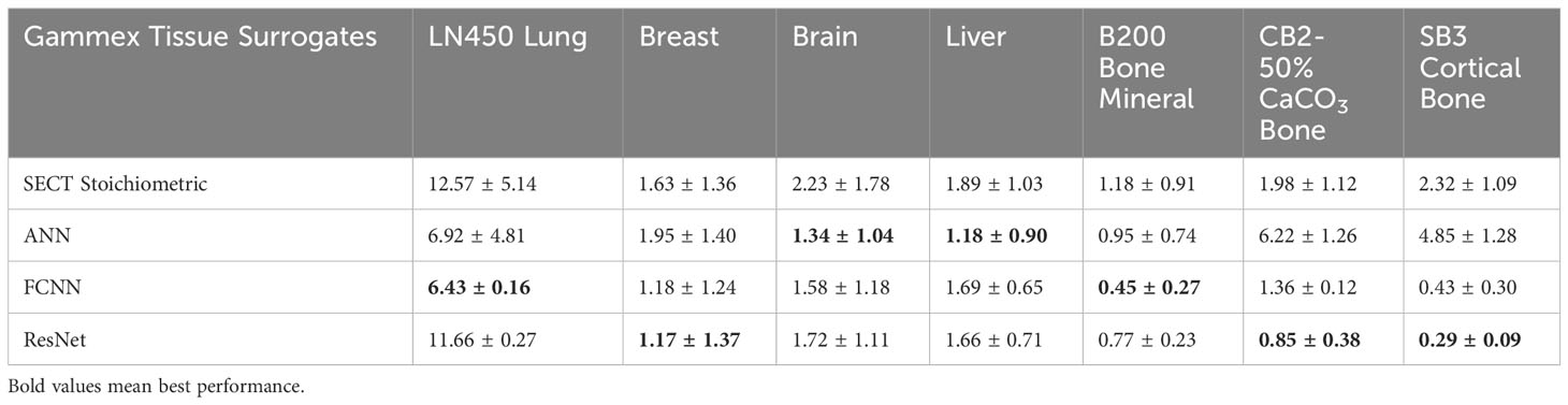
Table 4 Mass Density – MAPE [SECT DL vs. SECT stoichiometry].

TABLE 5

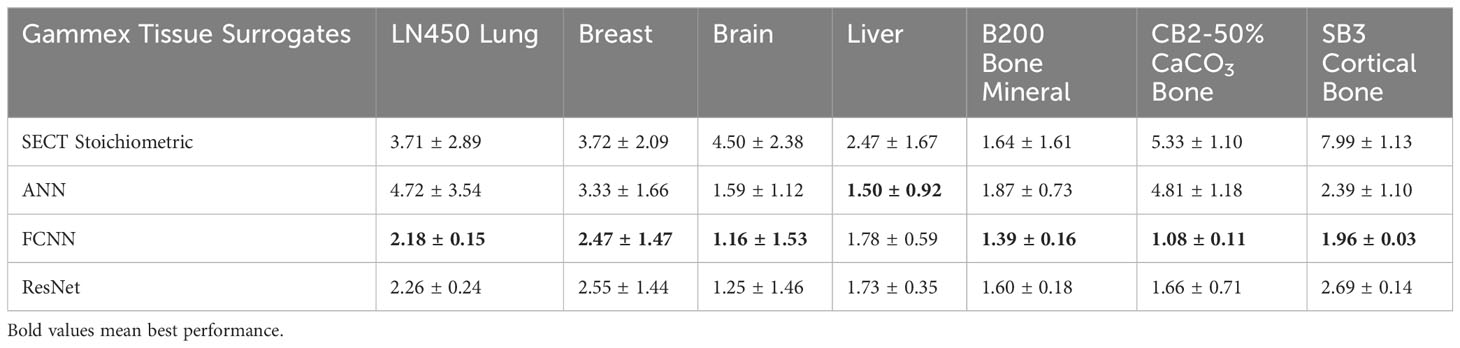
Table 5 RSP – MAPE [SECT DL vs. SECT stoichiometry].

3.2 HN site analysis using HN protocol

The mass densities and RSP predictions from the empirical model based on DECT parametric mapping, the SECT stoichiometric method, and the DL model results analysis are shown in Tables 6, 7. For all four tissues in M701, the DL methods are more accurate than the DECT empirical and SECT stoichiometric methods. The performance of FCNN and ResNet was comparable because of the similarity in the network fundamentals. For M702, the DECT empirical model outperforms the DL models in bone tissue prediction, which proves the advantage of DECT in bone tissue mass density estimation over SECT methods (ResNet has a comparable performance). However, this is not true for M701, the DL models based on SECT can achieve better results with the DECT empirical method in bone and other tissues. Table 7 summarizes the RSP MAPE comparison between the DECT empirical model, the stoichiometric method, and the DL models. For M701, DL methods outperform the traditional methods, while for M702, the DECT empirical method outperforms the DL methods in the spinal cord.

TABLE 6

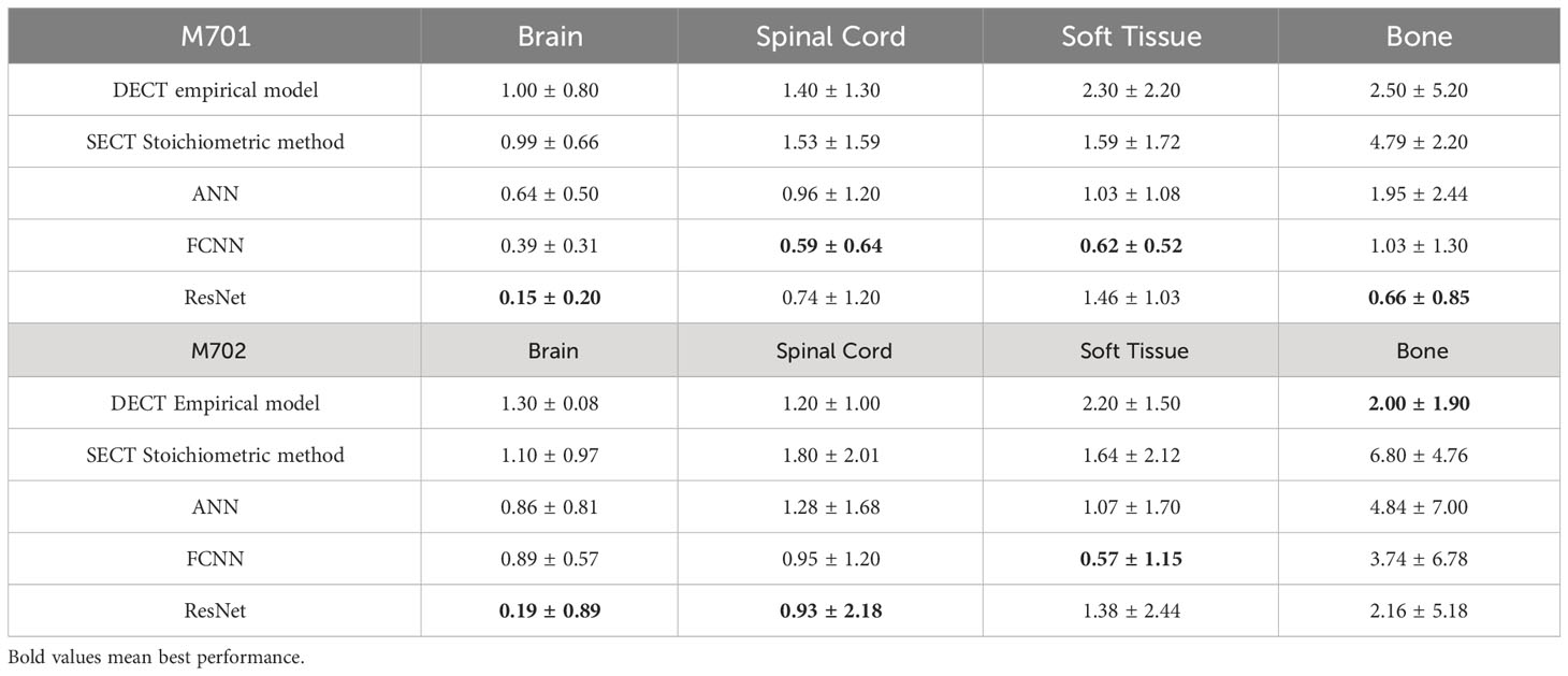
Table 6 Mass Density – MAPE [SECT DL vs. SECT stoichiometry vs. DECT model].

TABLE 7

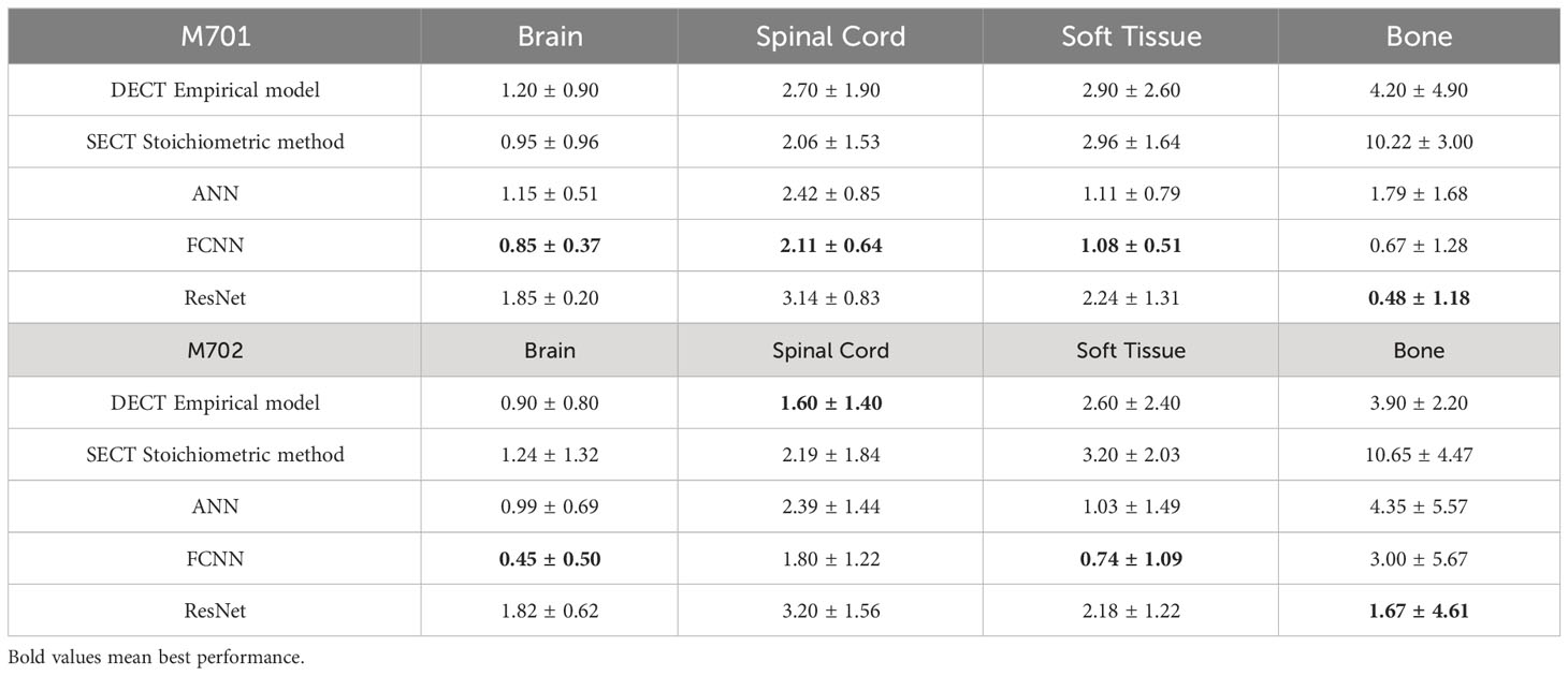
Table 7 RSP – MAPE [SECT DL vs. SECT stoichiometry vs. DECT model].

3.3 Chest site analysis using thorax protocol

Table 8 summarizes the MAPE comparison of mass density estimated by empirical and DL models on the chest site using 120 kVp thorax protocol. For the lung site, the DECT empirical model doesn’t apply to the normal lung tissue (the empirical model assigns the inflated lung as constant mass density), so the lung tissue mass density prediction is not reported. Table 9 shows the MAPE comparisons of RSP between the reference and DL models. All three DL models outperform the two reference models. The DECT empirical model and the stoichiometric method show better performance than ANN on lung tissue RSP prediction.

TABLE 8

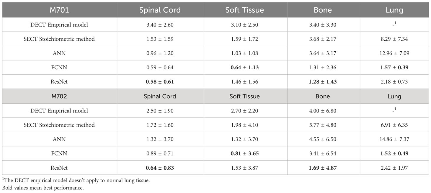
Table 8 Mass density – MAPE [SECT DL vs. SECT stoichiometry vs. DECT model].

TABLE 9

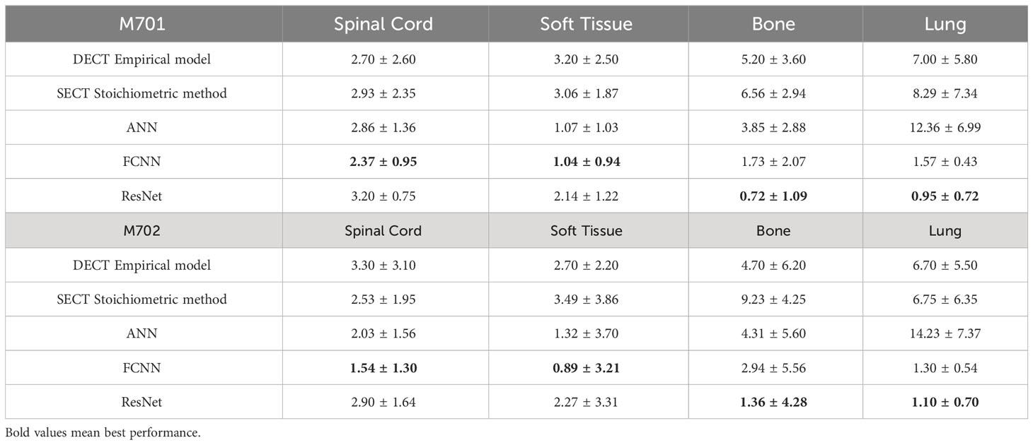
Table 9 RSP – MAPE [SECT DL vs. SECT stoichiometry vs. DECT model].

3.4 Pelvis site analysis using pelvis protocol

Table 10 shows the MAPE values of five models’ mass density predictions at the CIRS M701 and M702 phantom pelvis sites. DL methods show better performance in all three tissues and can reduce the error to<1% in the spinal cord and soft tissue. Table 11 shows the MAPE values of three DL models and the two reference models’ RSP estimations at the CIRS M701 and M702 phantom pelvis sites. The DL methods have better performance in soft tissue and bone, and all models have comparable results in the spinal cord.

TABLE 10

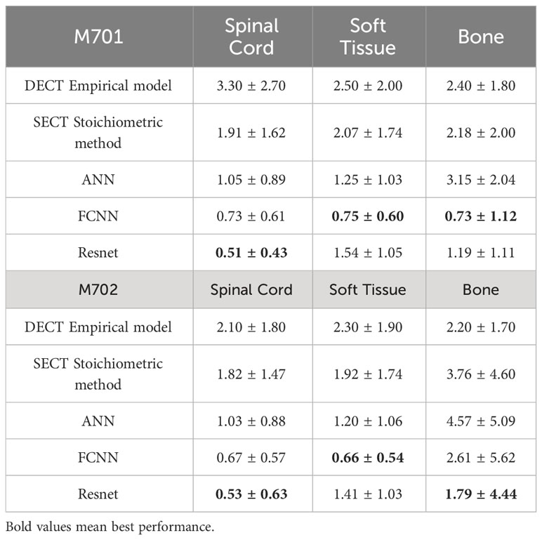
Table 10 Mass density – MAPE [SECT DL vs. SECT stoichiometry vs. DECT model].

TABLE 11

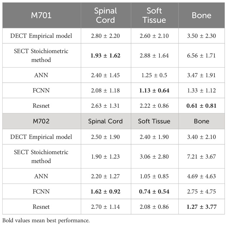
Table 11 RSP – MAPE [SECT DL vs. SECT stoichiometry vs. DECT model].

3.5 Whole phantom site analysis using HN, thorax, and pelvis protocols

Table 12 shows the MAPE comparisons of mass densities between DL models and the SECT stoichiometric method over the entire phantom site. Table 13 summarizes the MAPE comparisons of RSP between DL models and the SECT stoichiometric method over the entire phantom site.

TABLE 12

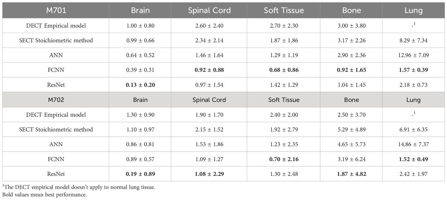
Table 12 Mass density – MAPE [SECT DL vs. SECT stoichiometry vs. DECT model].

TABLE 13

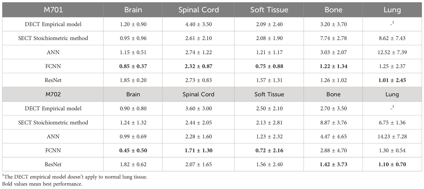
Table 13 RSP – MAPE [SECT DL vs. SECT stoichiometry vs. DECT model].

Figure 3 illustrates the APE maps of the mass density estimation error. Figures 3A17–C1 shows the SECT images of CIRS M701 phantom at three sites, HN, thorax, and pelvis, using 120 kVp corresponding scanning protocols. As presented using the APE color maps, the SECT stoichiometric model results in considerable uncertainty at lung and bone sites. Overall, the analysis for FCNN indicates the lowest error in the mass density estimation compared with other DL models. Figure 4 illustrates the APE maps for RSP error estimation. As with mass density, the SECT stoichiometric method shows considerable error in RSP estimation, especially in bone and lung tissue. ANN improves the estimation accuracy for bone and soft tissue, while FCNN predictions indicate improvements overall. ResNet shows smaller APE for bone, specifically for the pelvis scan, even when compared with FCNN.

FIGURE 3

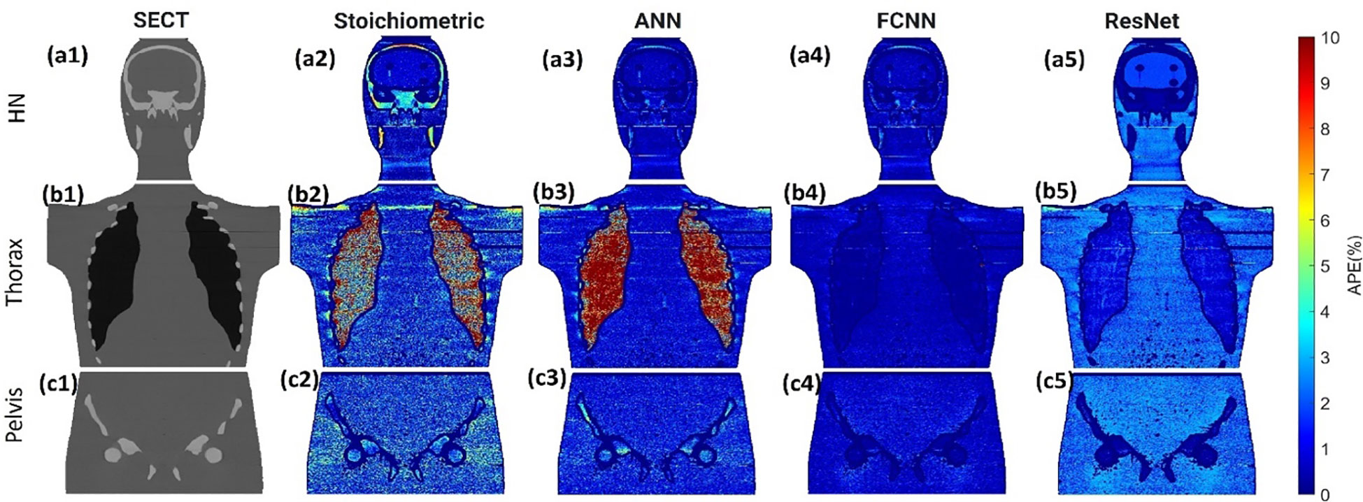
Figure 3 (A1, B1, C1) SECT images scan using different 120 kVp protocols. APE maps of mass densities between the reference and SECT parametric models at (A2–A5) HN, (B2–B5) thoracic, and (C2–C5) pelvic sites using CIRS M701 phantom.

FIGURE 4

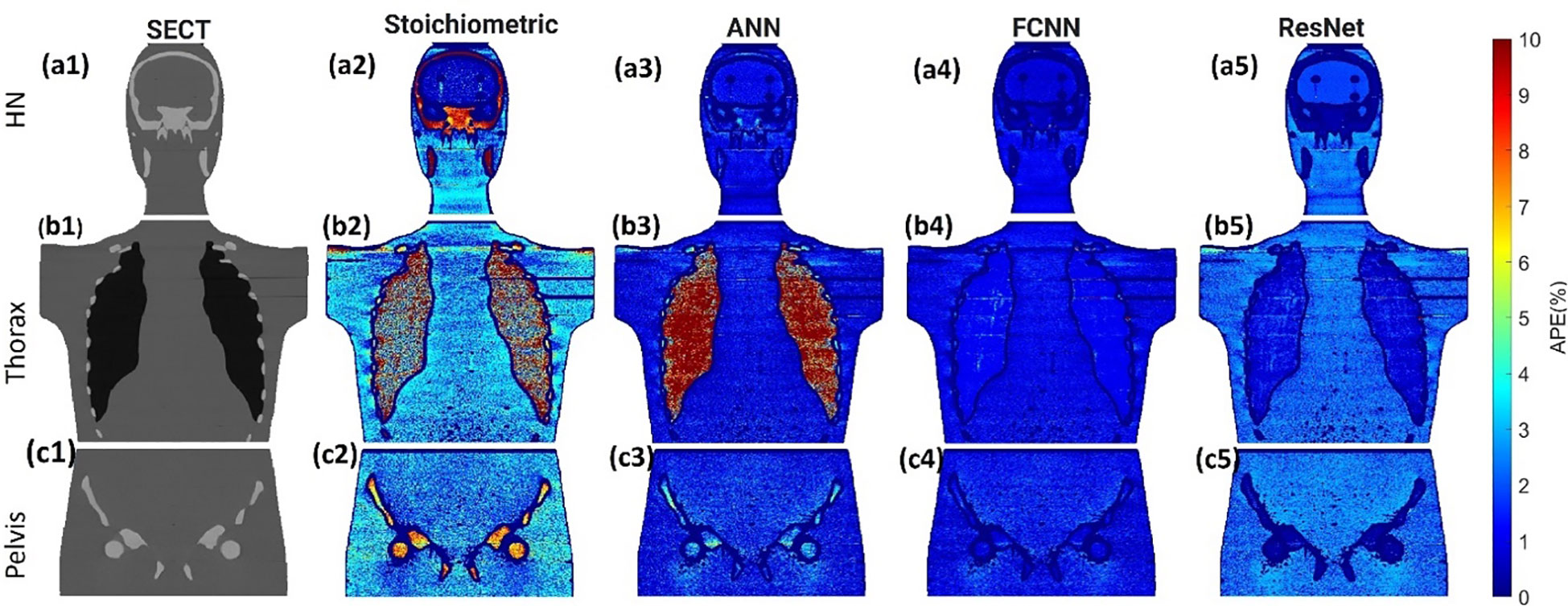
Figure 4 (A1, B1–C1) SECT images scan using different 120 kVp protocols. APE maps of RSP between the reference and SECT parametric models at (A2–A5) HN, (B2–B5) thoracic, and (C2–C5) pelvic sites using CIRS M701 phantom.

4 Discussions

External beam radiotherapy requires an accurate CT characterization of the patient geometry and heterogeneities to deliver accurate therapeutic patient doses. SECT imaging is the current clinical paradigm for generating the necessary information for clinical diagnosis and treatment planning in radiotherapy, including protons. Su et al. demonstrated the capability of machine learning methods to improve the prediction accuracy for mass density and RSP based on DECT imaging (18). In order to approach this methodology while using the more commonly available SECT imaging, we proposed a framework that can accurately predict mass density and RSP parametric maps for proton dose calculation while using SECT imaging as input. All SECT DL methods for mass density and RSP estimation were compared against the ground truth values defined in Table 1 and compared to current standards for mass density and RSP parametrization (DECT and stoichiometry). All parametrization was done on phantom data since the DL network training requires accurate ground truth definition, which excludes patient data. The DECT model MAPE was consistently larger than that of the SECT stoichiometric method for some of the tissues (specifically for the spinal cord). This could be attributed to the fact that the DECT empirical model depends on the relative electron density for mass density prediction and effective atomic number for RSP, and it has not been calibrated for the specific CT scanner used in this work. The SECT DL models demonstrated good or better performance for parametrization based on three different clinical scanning protocols (HN, Chest, Pelvic). Note that DL models were trained with phantom data, while the SECT stoichiometric method and DECT empirical data were optimized for clinical use with both phantom and human tissue, which might lead to worse performance on anthropomorphic phantom mass density and RSP estimation.

Gomà et al. concluded that the Gammex phantom utilized in this study contains tissue substitutes better representative of the human body than the CIRS electron density phantom (17). As shown in Tables 4, 5, we tested our DL models with Gammex 467 electron density phantom tissue surrogates, and the results indicate that the DL models can improve the mass density and RSP estimation relative to the stoichiometric method. Note that we tested our DL models on Gammex 467-1009 electron density phantom to evaluate the performance using different materials; then, we tested our DL models with CIRS M701&M702 phantoms for different materials and patient body sizes.

As shown in Figures 3, 4, the SECT stoichiometric method yields larger error in the lung, skull, pelvic bone, and soft tissue than DL networks. Also, the mass density and RSP maps generated with the SECT stoichiometric method have more noise than those generated by DL models, which indicates that DL models can handle noise and artifact suppression superiorly. It was reported that the uncertainty associated with mass density estimation dominates the proton range calculation uncertainty (7, 15, 32). In this work, DL models were trained with SECT images of electron density phantom, and Table 12 shows that the mass density MAPE can be improved significantly relative to the SECT stoichiometric method. The FCNN and ResNet outperform the ANN and reference models, and their MAPE values are close. A possible reason is that they share the same core network feature, the convolutional layer. Considering the training cost, the FCNN is recommended as the DL model for future dose calculation study. The RSP uncertainty is considerably larger than that of mass density, as demonstrated in Table 13, the DL models still exhibit the potential to enhance the accuracy of RSP estimation. FCNN could reduce the MAPE down to less than 2%, except in the spinal cord of CIRS M701.

Figure 5 illustrates the mass density prediction map generated by FCNN, ResNet, and the SECT stoichiometric method for two patients using HN and pelvis scans. As shown in Figures 5A3, A4, B3, B4, the DL models can reflect the patient’s anatomy qualitatively, compared with the SECT images in Figure 5A1. Figures 6A–C shows the comparison of CT number profile and density profile at the position marked in Figures 5A1, B1. Figures 6A–C demonstrates that the mass density profile generated by FCNN and ResNet has a strong agreement with the SECT number profile trend. As shown in Figures 5A2–A4, B2–B4, the mass density maps predicted by DL models have less noise than that predicted by the stoichiometric method, especially in the scan of the soft tissue of the pelvis. This implies that the DL models can suppress CT noises and artifacts, and it is also shown in the mass density profile comparison in Figure 6 that the DL models’ mass density lines are smoother than that of the stoichiometric method. The empirical model can provide better contrast information between adipose and bone tissue than the DL models; this might be because the DL models predict a higher density (~0.96 g/cm³) for adipose compared to the stoichiometric method (~0.88 g/cm³). The accurate density of the patient’s adipose tissue is not known; DL models estimated it at 8% higher than the stoichiometric method because the training dataset of the DL models doesn’t cover the mass density range from 0.5 to 0.95 g/cm³, while the clinically used SECT stoichiometric method CT curve has been calibrated with over 30 materials on various mass densities. If more tissue surrogates can be adapted into the training set of this framework, the robustness of DL models will be significantly improved. As shown in Figures 6A, C, FCNN has better performance in reproducing minor structure information from SECT images, such as the mass density difference in pelvic bone and bone marrow. Because ResNet has a complex model structure, including deep CNN layers, for example, when the dimension of data is insufficient (only SECT image as input), the complex model does not necessarily lead to a robust result (33).

FIGURE 5

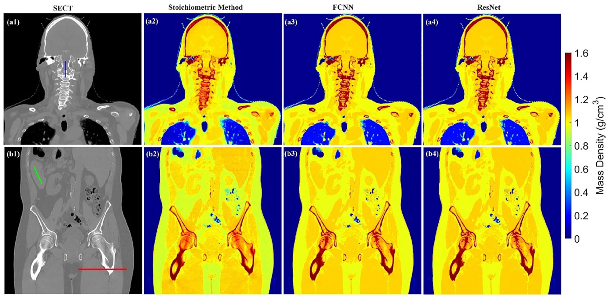
Figure 5 Mass density maps of two patients generated by different SECT FCNN and ResNet models at A1–A4 and B1–B4 using HN and pelvis scan.

FIGURE 6

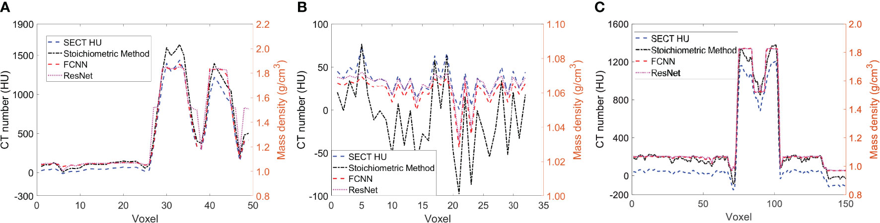
Figure 6 (A) the line profile from the blue line in Figure 5A1, (B) the line profile from green line in Figure 5B1, and (C) the line profile from the red line in Figure 5B1.

In supervised machine learning, a prevalent challenge is that DL models do not consistently generalize effectively from the training input data to new, unseen data (34). This overfitting phenomenon allows DL models to perform exemplarily in controlled conditions (similar or identical to the training conditions) while performing poorly on the application set. Many reasons can lead to this phenomenon, a lack of training dataset diversity being the predominant one. Only SECT phantom images were adapted into the training set; therefore, the DL networks’ infrastructure needed to be designed carefully to avoid overfitting. As shown in Figures 5, 6, the mass density profile estimated by DL models can basically follow the trend of SECT CT number and overlap with the profile of the SECT stoichiometric method. As shown in Table 14, DL models predicted a patient tissue mass density similar to that predicted using traditional methods. Integrating these findings, the design of the DL network successfully addresses and mitigates the overfitting issue.

TABLE 14

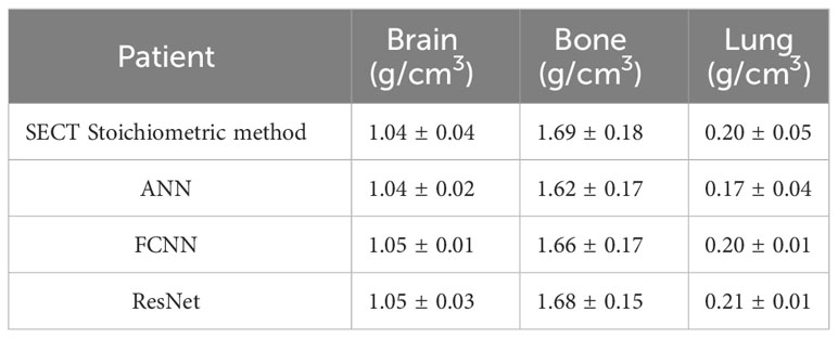
Table 14 Average mass density of three tissues comparison among DL models and the Stoichiometric model based on one patient SECT scan.

5 Conclusion

A DL framework was proposed to improve the mass density and RSP parametrization for proton dose calculation based on the SECT images. All three DL models outperform the SECT stoichiometric method in tissue substitute except the lung surrogate. FCNN and ResNet improved the mass density and RSP estimation accuracy based on SECT images, outperforming the SECT stoichiometric method over the entire phantom, and outperforming the DECT empirical model. DL models also demonstrate the ability to suppress CT image noise. The proposed DL frameworks have the potential to improve the clinical proton dose calculation based on SECT scans.

Data availability statement

The data analyzed in this study is subject to the following licenses/restrictions: The dataset can be available by contact the corresponding author. Requests to access these datasets should be directed to xyang43@emory.edu.

Ethics statement

The studies involving humans were approved by Emory University review board (IRB#114349). The studies were conducted in accordance with the local legislation and institutional requirements. The ethics committee/institutional review board waived the requirement of written informed consent for participation from the participants or the participants’ legal guardians/next of kin because this is a retrospective study, and the patient’s information was anonymized.

Author contributions

YG: Data curation, Investigation, Methodology, Writing – original draft, Writing – review & editing. C-WC: Investigation, Software, Validation, Writing – review & editing. JR: Writing – review & editing. MA: Writing – review & editing. YL: Methodology, Software, Writing – review & editing. SP: Methodology, Writing – review & editing. JB: Supervision, Writing – review & editing. JZ: Investigation, Methodology, Writing – review & editing. TL: Writing – review & editing. XY: Conceptualization, Funding acquisition, Investigation, Supervision, Writing – review & editing.

Funding

The author(s) declare financial support was received for the research, authorship, and/or publication of this article. This research is supported in part by the National Institutes of Health under Award Number R01CA215718, R56EB033332, and R01EB032680.

Conflict of interest

The authors declare that the research was conducted in the absence of any commercial or financial relationships that could be construed as a potential conflict of interest.

Publisher’s note

All claims expressed in this article are solely those of the authors and do not necessarily represent those of their affiliated organizations, or those of the publisher, the editors and the reviewers. Any product that may be evaluated in this article, or claim that may be made by its manufacturer, is not guaranteed or endorsed by the publisher.

References

1. Zhu J, Penfold SN. Dosimetric comparison of stopping power calibration with dual-energy CT and single-energy CT in proton therapy treatment planning. Med Phys (2016) 43:2845–54. doi: 10.1118/1.4948683

PubMed Abstract | CrossRef Full Text | Google Scholar

2. Schneider U, Pedroni E, Lomax A. The calibration of CT Hounsfield units for radiotherapy treatment planning. Phys Med Biol (1996) 41:111–24. doi: 10.1088/0031-9155/41/1/009

PubMed Abstract | CrossRef Full Text | Google Scholar

3. Woodard HQ, White DR. The composition of body tissues. Br J Radiol (1986) 59:1209–18. doi: 10.1259/0007-1285-59-708-1209

PubMed Abstract | CrossRef Full Text | Google Scholar

4. International Commission On Radiation, U. & Measurements B. M. D. Tissue substitutes in radiation dosimetry and measurement. (Bethesda, MD (United States): International Commission on Radiation Units and Measurements) (1989). Available at: https://www.osti.gov/biblio/10102048.

Google Scholar

5. Scott JA. Photon, electron, proton and neutron interaction data for body tissues ICRU report 46. International commission on radiation units and measurements, Bethesda 1992, $40.00. J Nucl Med (1993) 34:171–1.

Google Scholar

6. McCollough CH, Boedeker K, Cody D, Duan X, Flohr T, Halliburton SS, et al. Principles and applications of multienergy CT: Report of AAPM Task Group 291. Med Phys (2020) 47:4. doi: 10.1002/mp.14157

CrossRef Full Text | Google Scholar

7. Hunemohr N, Krauss B, Tremmel C, Ackermann B, Jakel O, Greilich S. Experimental verification of ion stopping power prediction from dual energy CT data in tissue surrogates. Phys Med Biol (2014) 59:83–96. doi: 10.1088/0031-9155/59/1/83

PubMed Abstract | CrossRef Full Text | Google Scholar

8. Paganetti H. Range uncertainties in proton therapy and the role of Monte Carlo simulations. Phys Med Biol (2012) 57:R99–117. doi: 10.1088/0031-9155/57/11/R99

PubMed Abstract | CrossRef Full Text | Google Scholar

9. Paganetti H, Jiang H, Parodi K, Slopsema R, Engelsman M. Clinical implementation of full Monte Carlo dose calculation in proton beam therapy. Phys Med Biol (2008) 53:4825–53. doi: 10.1088/0031-9155/53/17/023

PubMed Abstract | CrossRef Full Text | Google Scholar

10. Taasti VT, Bäumer C, Dahlgren CV, Deisher AJ, Ellerbrock M, Free J, et al. Inter-centre variability of CT-based stopping-power prediction in particle therapy: Survey-based evaluation. Phys Imaging Radiat Oncol (2018) 6:25–30. doi: 10.1016/j.phro.2018.04.006

PubMed Abstract | CrossRef Full Text | Google Scholar

11. Chang CW, Huang S, Harms J, Zhou J, Zhang R, Dhabaan A, et al. A standardized commissioning framework of Monte Carlo dose calculation algorithms for proton pencil beam scanning treatment planning systems. Med Phys (2020) 47:1545–57. doi: 10.1002/mp.14021

PubMed Abstract | CrossRef Full Text | Google Scholar

12. Peters N, Wohlfahrt P, Dahlgren CV, De Marzi L, Ellerbrock M, Fracchiolla F, et al. Experimental assessment of inter-centre variation in stopping-power and range prediction in particle therapy. Radiother Oncol (2021) 163:7–13. doi: 10.1016/j.radonc.2021.07.019

PubMed Abstract | CrossRef Full Text | Google Scholar

13. Paganetti H. Monte Carlo simulations will change the way we treat patients with proton beams today. Br J Radiol (2014) 87:20140293. doi: 10.1259/bjr.20140293

PubMed Abstract | CrossRef Full Text | Google Scholar

14. Bourque AE, Carrier J-F, Bouchard H. A stoichiometric calibration method for dual energy computed tomography. Phys Med Biol (2014) 59:2059–88. doi: 10.1088/0031-9155/59/8/2059

PubMed Abstract | CrossRef Full Text | Google Scholar

15. Yang M, Virshup G, Clayton J, Zhu XR, Mohan R, Dong L. Theoretical variance analysis of single- and dual-energy computed tomography methods for calculating proton stopping power ratios of biological tissues. Phys Med Biol (2010) 55:1343–62. doi: 10.1088/0031-9155/55/5/006

PubMed Abstract | CrossRef Full Text | Google Scholar

16. Wohlfahrt P, Mohler C, Hietschold V, Menkel S, Greilich S, Krause M, et al. Clinical implementation of dual-energy CT for proton treatment planning on pseudo-monoenergetic CT scans. Int J Radiat Oncol Biol Phys (2017) 97:427–34. doi: 10.1016/j.ijrobp.2016.10.022

PubMed Abstract | CrossRef Full Text | Google Scholar

17. Gomà C, Almeida IP, Verhaegen F. Revisiting the single-energy CT calibration for proton therapy treatment planning: a critical look at the stoichiometric method. Phys Med Biol (2018) 63:235011. doi: 10.1088/1361-6560/aaede5

PubMed Abstract | CrossRef Full Text | Google Scholar

18. Su KH, Kuo JW, Jordan DW, Van Hedent S, Klahr P, Wei Z, et al. Machine learning-based dual-energy CT parametric mapping. Phys Med Biol (2018) 63:125001. doi: 10.1088/1361-6560/aac711

PubMed Abstract | CrossRef Full Text | Google Scholar

19. Schmidhuber J. Deep learning in neural networks: An overview. Neural Networks (2015) 61:85–117. doi: 10.1016/j.neunet.2014.09.003

PubMed Abstract | CrossRef Full Text | Google Scholar

20. Sahiner B, Pezeshk A, Hadjiiski LM, Wang X, Drukker K, Cha KH, et al. Deep learning in medical imaging and radiation therapy. Med Phys (2019) 46:e1–e36. doi: 10.1002/mp.13264

PubMed Abstract | CrossRef Full Text | Google Scholar

21. Lecun Y, Bengio Y, Hinton G. Deep learning. Nature (2015) 521:436–44. doi: 10.1038/nature14539

PubMed Abstract | CrossRef Full Text | Google Scholar

22. Chang C-W, Gao Y, Wang T, Lei Y, Wang Q, Pan S, et al. Dual-energy CT based mass density and relative stopping power estimation for proton therapy using physics-informed deep learning. Phys Med Biol (2022) 67(11):115010. doi: 10.1088/1361-6560/ac6ebc

CrossRef Full Text | Google Scholar

23. Hassoun MH. Fundamentals of artificial neural networks. Cambridge, Massachusetts, United States: MIT press (1995).

Google Scholar

24. Krizhevsky A, Sutskever I, Hinton GE. Imagenet classification with deep convolutional neural networks. Adv Neural Inf Process Syst (2012) 25.

PubMed Abstract | Google Scholar

25. He K, Zhang X, Ren S, Sun J. Identity mappings in deep residual networks. In Computer Vision–ECCV 2016: 14th European Conference, Amsterdam, The Netherlands, October 11–14, 2016, Proceedings, Part IV 14. (Springer International Publishing) (2016), 630–45.

Google Scholar

26. Paszke A, Gross S, Massa F, Lerer A, Bradbury J, Chanan G, et al. Pytorch: An imperative style, high-performance deep learning library. Adv Neural Inf Process Syst (2019) 32.

Google Scholar

27. Kiranyaz S, Avci O, Abdeljaber O, Ince T, Gabbouj M, Inman DJ. 1D convolutional neural networks and applications: A survey. Mechanical Syst Signal Process (2021) 151:107398. doi: 10.1016/j.ymssp.2020.107398

CrossRef Full Text | Google Scholar

28. Rutherford RA, Pullan BR, Isherwood I. Measurement of effective atomic number and electron density using an EMI scanner. Neuroradiology (1976) 11:15–21. doi: 10.1007/BF00327253

PubMed Abstract | CrossRef Full Text | Google Scholar

29. Bichsel H. Passage of charged particles through matter. California Univ., Berkeley (USA), Dept. of Physics: Office of Scientific and Technical Information (OSTI) (1969).

Google Scholar

30. Deasy J. ICRU report 49, stopping powers and ranges for protons and alph particles. Med Phys (1994) 21:709–10. doi: 10.1118/1.597176

CrossRef Full Text | Google Scholar

31. Beaulieu L, Tedgren Å.C, Carrier J-F, Davis SD, Mourtada F, Rivard MJ, et al. Report of the Task Group 186 on model-based dose calculation methods in brachytherapy beyond the TG-43 formalism: Current status and recommendations for clinical implementation. Med Phys (2012) 39:6208–36. doi: 10.1118/1.4747264

PubMed Abstract | CrossRef Full Text | Google Scholar

32. Yang M, Zhu XR, Park PC, Titt U, Mohan R, Virshup G, et al. Comprehensive analysis of proton range uncertainties related to patient stopping-power-ratio estimation using the stoichiometric calibration. Phys Med Biol (2012) 57:4095–115. doi: 10.1088/0031-9155/57/13/4095

PubMed Abstract | CrossRef Full Text | Google Scholar

33. Chang C-W, Dinh NT. Classification of machine learning frameworks for data-driven thermal fluid models. Int J Thermal Sci (2019) 135:559–79. doi: 10.1016/j.ijthermalsci.2018.09.002

CrossRef Full Text | Google Scholar

34. Ying X. An overview of overfitting and its solutions. J Physics: Conf Ser (2019) 1168:022022. doi: 10.1088/1742-6596/1168/2/022022

CrossRef Full Text | Google Scholar