Encoding-independent optimization problem formulation for quantum computing

1 Introduction

Discrete optimization problems are ubiquitous in almost any enterprise and many of these are known to be NP-hard (Lenstra and Rinnooy Kan, 1979). The objective of such problems is to find the minimum of a real-valued function f(v₀, …, v_N−1) (the cost function) over a set of discrete variables v_k. The search space is restricted by hard constraints, which are commonly presented as equalities such as g(v₀, …, v_N−1) = 0 or inequalities as h(v₀, …, v_N−1) > 0. Besides using classical heuristics (Dorigo and Di Caro, 1999; Melnikov, 2005) and machine learning methods (Mazyavkina et al., 2021) to solve these problems, there is a growing interest in applying quantum computation (Au-Yeung et al., 2023). A common approach for realizing this consists of first encoding the cost function f in a Hamiltonian H such that a subset of eigenvectors of H represents elements in the domain of f and the eigenvalues are the respective values of f:

$H\left|\psi \right.⟩=f\left(v_0,\dots ,v_{N-1}\right)\left|\psi \right.⟩.(1)$

In such an encoding, the ground state of H is the solution to the optimization problem. Having obtained a Hamiltonian formulation, one can use a variety of quantum algorithms to find the ground state including adiabatic quantum computing (Farhi et al., 2000) and variational approaches, for instance, the quantum/classical hybrid quantum approximate optimization algorithm (QAOA) (Farhi et al., 2014) or generalizations thereof such as the quantum alternating operator ansatz (Hadfield et al., 2019). On the hardware side, these algorithms can run on gate-based quantum computers, quantum annealers, or specialized Ising machines (Mohseni et al., 2022).

In the current literature, almost all Hamiltonians for optimization are formulated as Quadratic Unconstrained Binary Optimization (QUBO) problems (Kochenberger et al., 2014). The success of QUBO reflects the strong hardware limitations of current devices, where multiqubit interactions are not available and must be decomposed into two-qubit interactions using ancilla qubits. Moreover, quantum algorithms with the dynamical implementation of hard constraints (Hen and Sarandy, 2016; Hen and Spedalieri, 2016) require driver terms that can be difficult to design and implement on quantum computers. Hence, hard constraints are usually included as energy penalizations of QUBO Hamiltonians. The prevalence of QUBO has also increased the popularity of one-hot encoding, a particular way of mapping (discrete) variables to eigenvalues of spin operators (Lucas, 2014), since this encoding allows for Hamiltonians with low-order interactions which is especially appropriate for QUBO problems.

However, compelling alternatives to QUBO and one-hot encoding have been proposed in recent years. A growing number of platforms are exploring high-order interactions (Chancellor et al., 2017; Lu et al., 2019; Schöndorf and Wilhelm, 2019; Wilkinson and Hartmann, 2020; Menke et al., 2021; 2022; Dlaska et al., 2022; Pelegrí et al., 2022; Glaser et al., 2023), while the Parity architecture (Lechner, 2020; Fellner et al., 2022; Ender et al., 2023) (a generalization of the LHZ architecture (Lechner et al., 2015)) allows the mapping of arbitrary-order interactions to qubits that require only local connectivity. The dynamical implementation of constraints has also been investigated (Hadfield et al., 2019; 2017; Fuchs et al., 2022; Zhu et al., 2023), including the design of approximate drivers (Wang et al., 2020; Sawaya et al., 2022) and compilation of constrained problems within the Parity architecture (Drieb-Schön et al., 2023). Moreover, simulated and experimental results have shown that alternative encodings outperform the traditional one-hot approach (Chancellor, 2019; Sawaya et al., 2020; Chen et al., 2021; Plewa et al., 2021; Tamura et al., 2021; Glos et al., 2022; Stein et al., 2023). Clearly, alternative formulations for Hamiltonians need to be explored but when the Hamiltonian has been expressed in QUBO using one-hot encoding, it is not trivial to switch to other formulations. Automatic tools to explore different formulations would therefore be highly beneficial.

We present a library of more than 20 problems which is intended to facilitate the Hamiltonian formulation beyond QUBO and one-hot encoding. We build upon the recent work of Sawaya et al. (2022) by making use of the encoding-independent approach to revisit common problems in the literature. With this approach, the problems can be encoded trivially using any spin encoding. We also provide a summary of the most popular encodings. Possible constraints of the problems are identified and presented separately from the cost function so that dynamic implementation of the constraints can also be easily explored. Two additional subgoals that are addressed in this library are:

• Meta parameters/choices: We present and review the most important choices made in the process of mapping optimization problems in a mathematical formulation to spin Hamiltonians. These mainly include the encodings, which can greatly influence the computational cost and performance of the optimization, but also free meta parameters or the use of auxiliary variables. These degrees of freedom are a consequence of the fact that the optimal solution is typically encoded only in the ground state. Other low-energy eigenstates encode good approximations to the optimal solution and it can be convenient to make approximations so that the solution corresponds to these states (Montanez-Barrera et al., 2022).

• (Partial) automation: Usually, each problem needs to be evaluated individually. The resulting cost functions are not necessarily unique and there is no known trivial way of automatically creating H. By providing a collection of building blocks of cost functions and heuristics for selecting parameters, the creation of the cost function and constraints is assisted. This enables a general representation of problems in an encoding-independent way and parts of the parameter selection and performance analysis can be conducted at this intermediate stage. This goal has also been discussed by Sawaya et al. (2022).

In practice, many optimization problems are not purely discrete but involve real-valued parameters and variables. Thus, the encoding of real-valued problems to discrete optimization problems (discretization) as an intermediate step is discussed in Section 7.4.

The focus of this review is on optimization problems which can be formulated as diagonal Hamiltonians written as sums and products of Pauli-z-matrices. This subset of Hamiltonians is usually not applicable to quantum systems or quantum simulations. For an introduction to these more general Hamiltonians, we refer to the reviews of Georgescu et al. (2014) for physics problems and McArdle et al. (2020); Cao et al. (2019) for quantum chemistry simulations.

After introducing the notation used throughout the text in Section 2, we present a list of encodings in Section 3. Section 4 reviews the Parity architecture and Section 5 discusses encoding constraints. Section 6 functions as a manual on how to bring optimization problems into a form that can be solved with a quantum computer. Section 7 contains a library of optimization problems which are classified into several categories and Section 8 lists the building blocks used in the formulation of these (and many other) problems. Section 9 offers conclusions.

2 Definitions and notation

A discrete set of real numbers is a countable subset $U\subset \mathbb{R}$ without an accumulation point. Discrete sets are denoted by uppercase Latin letters, except the letter G, which we reserve for graphs. A discrete variable is a variable ranging over a discrete set R and will be represented by lowercase Latin letters, mostly v or w. Elements of R are denoted by lowercase Greek letters.

If a discrete variable has range $\left\{\mathrm{0,1}\right\}$ we call it binary or boolean. Binary variables will be denoted by the letter x. Similarly, a variable with range $\left\{-\mathrm{1,1}\right\}$ will be called a spin variable and the letter s will be reserved for these. There is an invertible mapping from a binary variable x to a spin variable s:

$x\mapsto s:=2x-1.(2)$

For a variable v with range R we follow Chancellor (2019) and Sawaya et al. (2022) and define the value indicator function to be

${\delta }_v^{\alpha }=\left\{\begin{array}{c}1\mathrm{i}\mathrm{f}v=\alpha \hfill \\ 0\mathrm{i}\mathrm{f}v\ne \alpha ,\hfill \end{array}\right.(3)$

where α ∈ R.

We also consider optimization problems for continuous variables. A variable v will be called continuous, if its range is given by ${\mathbb{R}}^d$ for some $d\in {\mathbb{Z}}_{>0}$.

An optimization problem O is a triple (V, f, C), where.

1. $V:={\left\{v_i\right\}}_{i=0,\dots ,N-1}$ is a finite set of variables.

2. f := f(v₀, …, v_N−1) is a real-valued function, called objective or cost function.

3. $C={\left\{C_i\right\}}_{i=0,\dots ,l}$ is a finite set of constraints C_i. A constraint C is either an equation

$c\left(v_0,\dots ,v_{N-1}\right)=k(4)$

for some $k\in \mathbb{R}$ and a real-valued function c(v₀, …, v_N−1), or it is an inequality

$c\left(v_0,\dots ,v_{N-1}\right)\le k.(5)$

The goal for an optimization problem O = (V, f, C) is to find an extreme value y_ex of f, such that all of the constraints are satisfied at y_ex.

Discrete optimization problems can often be stated in terms of graphs or hypergraphs (Berge, 1987). A graph is a pair (V, E), where V is a finite set of vertices or nodes and $E\subset \left\{\left\{v_i,v_j\right\}|v_i\ne v_j\in V\right\}$ is the set of edges. An element $\left\{v_i,v_j\right\}\in E$ is called an edge between vertex v_i and vertex v_j. Note that a graph defined like this can neither have loops, i.e., edges beginning and ending at the same vertex, nor can there be multiple edges between the same pair of vertices. Given a graph G = (V, E), its adjacency matrix is the symmetric binary |V|×|V| matrix A with entries

$A_{ij}=\left\{\begin{array}{cc}1,\hfill & \text{if}\left\{v_i,v_j\right\}\in E,\hfill \\ 0,\hfill & \text{else}.\hfill \end{array}\right.(6)$

A hypergraph is a generalization of a graph in which we allow edges to be adjacent to more than two vertices. That is, a hypergraph is a pair H = (V, E), where V is a finite set of vertices and

$\begin{array}{cc}\hfill E\subseteq \bigcup _{i=1}^{|V|}\left\{\{v_{j_1},\dots ,v_{j_i}\}\right.|v_{j_k}\in V& \mathrm{a}\mathrm{n}\mathrm{d}{v}_{j_k}\ne v_{j_{\ell }}\hfill \\ \hfill & \left.\forall k,\ell =1,\cdots i\right\}\hfill \end{array}(7)$

is the set of hyperedges.

We reserve the word qubit for physical qubits. To go from an encoding-independent Hamiltonian to a quantum program, binary or spin variables become Pauli-z-matrices which act on the corresponding qubits.

3 Encodings library

For many problems, the cost function and the problem constraints can be represented in terms of two fundamental building blocks: the value of the integer variable v and the value indicator ${\delta }_v^{\alpha }$ defined in Eq. 3. When expressed in terms of these building blocks, Hamiltonians are more compact, and recurring terms can be identified across many different problems. Moreover, quantum operators are not present at this stage: an encoding-independent Hamiltonian is just a cost function in terms of discrete variables, which eases access to quantum optimization to a wider audience. Encoding variables and the choice of quantum algorithms can come later.

Representation of the building blocks in terms of Ising operators depends on the chosen encoding. An encoding is a function that associates eigenvectors of the σ_z operator with specific values of a discrete variable v:

$|s_0,\dots ,s_{N-1}\rangle \to v,s_i=\pm 1,(8)$

where the spin variables s_i are the eigenvalues of ${\sigma }_z^{(i)}$ operators. The encodings are also usually defined in terms of binary variables x_i which are related to Ising variables according to Eq. 2.

A summary of the encodings is presented in Figure 1. Some encodings are dense, in the sense that every quantum state |s₀, …, s_N−1⟩ encodes some value of the variable v. Other encodings are sparse because only a subset of the possible quantum states are valid states. The valid subset is generated by adding a core term¹, i.e., a penalty term for constraints that need to be enforced in order to decode the variable uniquely in the Hamiltonian for every sparsely encoded variable. In general, dense encodings require fewer qubits, but sparse encodings have simpler expressions for the value indicator ${\delta }_v^{\alpha }$, and are therefore favorable for avoiding higher-order interactions. This is because ${\delta }_v^{\alpha }$ needs to check a smaller number of qubit states to know whether the variable v has value α or not, whereas dense encodings require the state of every qubit in the register (Sawaya et al., 2020; 2022).

FIGURE 1

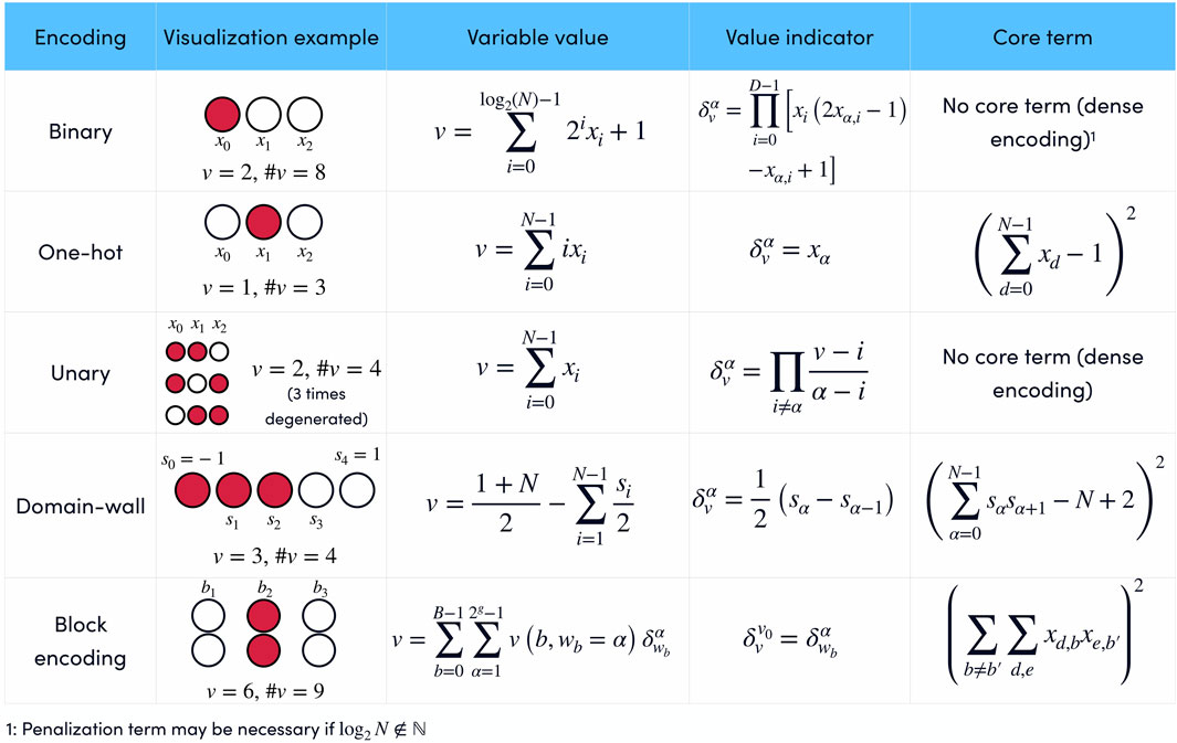
FIGURE 1. Summary of popular encodings of discrete variables in terms of binary x_i or Ising s_i variables. Each encoding has a particular representation of the value of the variable v and the value indicator ${\delta }_v^{\alpha }$. We also include a visualization example for each encoding, where the red circles represent excited qubits and #v is the range of variable v for the given number of qubits. If every quantum state in the register represents a valid value of v, the encoding is called dense. On the contrary, sparse encodings must include a core term in the Hamiltonian in order to represent a value of v. Sparse encodings have simpler representations of the value indicators than dense encodings, but the core term implementation demands extra interaction terms between the qubits. The cost of a Hamiltonian in terms of the number of qubits and interaction terms strongly depends on the chosen encoding and should be evaluated for every specific problem.

3.1 Binary encoding

Binary encoding uses the binary representation for encoding integer variables. Given an integer variable $v\in \left[1,2^D\right]$, we can use D binary variables x_i ∈ {0, 1} to represent v:

$v={\displaystyle \sum _{i=0}^{D-1}}{2}^i{x}_i+1.(9)$

The value indicator ${\delta }_v^{\alpha }$ can be written using the generic expression

${\delta }_v^{\alpha }={\displaystyle \prod _{i\ne \alpha }}\frac{v-i}{\alpha -i},(10)$

which is valid for every encoding. The expression for ${\delta }_v^{\alpha }$ in terms of boolean variables x_i can be written using that the value of α is codified in the bitstring (x_α,0…, x_α,D−1). The value indicator ${\delta }_v^{\alpha }$ checks if the D binary variables x_i are equal to x_α,i to know if the variable v has the value α or not. We note that

$x_1\left(2x_2-1\right)-x_2+1=\left\{\begin{array}{c}1\mathrm{i}\mathrm{f}{x}_1=x_2\hfill \\ 0\mathrm{i}\mathrm{f}{x}_1\ne x_2\hfill \end{array}\right.(11)$

and so we write

$\begin{array}{cc}\hfill {\delta }_v^{\alpha }& ={\displaystyle \prod _{i=0}^{D-1}}\left[x_i\left(2x_{\alpha ,i}-1\right)-x_{\alpha ,i}+1\right]\hfill \\ \hfill & ={\displaystyle \prod _{i=0}^{D-1}}{s}_i\left(x_{\alpha ,i}-\frac{1}{2}\right)+\frac{1}{2},\hfill \end{array}(12)$

where

$s_i=2x_i-1(13)$

are the corresponding Ising variables. Thus, the maximum order of the interaction terms in ${\delta }_v^{\alpha }$ scales linearly with D and there are $\left(\genfrac{}{}{0.0pt}{}{D}{k}\right)$ terms of order k. The total number of terms is ${\sum }_k\left(\genfrac{}{}{0.0pt}{}{D}{k}\right)=2^D$ and the number of interaction terms needed for a value indicator in binary encoding scales linearly with the maximum value of the variable N = 2^D.

If v ∈ {1, …, K} with $2^D<K<2^{D+1},D\in \mathbb{N}$, then we require D + 1 binary variables to represent v and we will have 2^D+1 − K invalid quantum states that do not represent any value of the variable v. The set of invalid states is

$R=\left\{|\mathbf{x}\rangle \left|{\displaystyle \sum _{i=0}^D}{2}^i{x}_i+1>K\right.\right\}.(14)$

for rejecting quantum states in R, we can force v ≤ K, which can be accomplished by adding a core term H_core in the Hamiltonian

$H_{\text{core}}={\displaystyle \sum _{\alpha =K+1}^{2^{D+1}}}{\delta }_v^{\alpha },(15)$

or imposing the sum constraint

$c_{\text{core}}={\displaystyle \sum _{\alpha =K+1}^{2^{D+1}}}{\delta }_v^{\alpha }=0(16)$

The core term penalizes any state that represents an invalid value for variable v. Because core terms impose an additional energy scale, the performance can reduce when $K\ne 2^D,D\in \mathbb{N}$. In some cases, such as the Knapsack problem, penalties for invalid states can be included in the cost function, so there is no need to add a core term or constraints (Tamura et al., 2021) (Section 8.2.3).

When encoding variables that can also take on negative values, e.g., v ∈ {− K, − K + 1, …, K′ − 1, K′}, in classical computing one often uses an extra bit that encodes the sign of the value. However, this might not be the best option because one spin flip could then change the value substantially and we do not assume full fault tolerance. For binary encoding there is a more suitable treatment of negative values: we can simply shift the values

$v={\displaystyle \sum _{i=0}^{D-1}}{2}^i{x}_i+1-K,(17)$

where 2^D−1 < K + K′ ≤ 2^D. The expression for the value indicator functions stays the same, only the encoding of the value α has to be adjusted. An additional advantage over using the sign bit is that ranges that are not symmetrical around zero (K ≠ K′) can be encoded more efficiently. The same approach of shifting the variable by −K can also be used for the other encodings.

3.2 Gray encoding

In binary representation, a single spin flip can lead to a sharp change in the value of v, for example, |1000⟩ codifies v = 9 while |0000⟩ codifies v = 1. To avoid this, Gray encoding reorders the binary representation in a way that two consecutive values of v always differ in a single spin flip. If we line up the potential values v ∈ [1, 2^D] of an integer variable in a vertical sequence, this encoding in D boolean variables can be described as follows: on the ith boolean variable (which is the ith column from the right) the sequence starts with 2ⁱ⁻¹ zeros and continues with an alternating sequence of 2ⁱ 1s and 2ⁱ 0s. As an example, consider

$\begin{array}{ll}\hfill 1:& 0000\hfill \\ \hfill 2:& 0001\hfill \\ \hfill 3:& 0011\hfill \\ \hfill 4:& 0010\hfill \\ \hfill 5:& 0110\hfill \\ \hfill 6:& 0111\hfill \\ \dots \hfill \end{array}$

where D = 4. On the left-hand side of each row of boolean variables, we have the value v. If we, for example, track the right-most boolean variable, we indeed find that it starts with 2^1–1 = 1 zero for the first value, 2¹ ones for the second and third values, 2¹ zeros for the third and fourth values, and so on.

The value indicator function and the core term remain unchanged except that the representation of, for example, α in the analog of Eq. 12 also has to be in Gray encoding.

An advantage of this encoding with regard to quantum algorithms is that single spin flips do not cause large changes in the cost function and thus smaller coefficients may be chosen (see discussion in Section 8). The advantage of using Gray over one-hot encoding was recently demonstrated for quantum simulations of a deuteron (Di Matteo et al., 2021).

3.3 One-hot encoding

One-hot encoding is a sparse encoding that uses N binary variables x_α to encode an N-valued variable v. The encoding is defined by its variable indicator:

${\delta }_v^{\alpha }=x_{\alpha },(18)$

which means that v = α if x_α = 1. The value of v is given by

$v={\displaystyle \sum _{\alpha =0}^{N-1}}\alpha x_{\alpha }.(19)$

The physically meaningful quantum states are those with a single qubit in state 1 and so the dynamics must be restricted to the subspace defined by

$c_{\text{core}}={\displaystyle \sum _{\alpha =0}^{N-1}}{x}_{\alpha }-1=0.(20)$

One option to impose this sum constraint is to encode it as an energy penalization with a core term in the Hamiltonian:

$H_{\text{core}}={\left(1-{\displaystyle \sum _{\alpha =0}^{N-1}}{x}_{\alpha }\right)}^2,(21)$

which has minimum energy if only one x_α is different from zero.

3.4 Domain-wall encoding

This encoding uses the position of a domain wall in an Ising chain to codify values of a variable v (Chancellor, 2019; Berwald et al., 2023). If the endpoints of an N + 1 spin chain are fixed in opposite states, there must be at least one domain wall in the chain. Since the energy of a ferromagnetic Ising chain depends only on the number of domain walls it has and not on where they are located, an N + 1 spin chain with fixed opposite endpoints has N possible ground states, depending on the position of the single domain wall.

The codification of a variable v = 1, …, N using domain wall encoding requires the core Hamiltonian Chancellor (2019):

$H_{\text{core}}=-\left[-s_1+{\displaystyle \sum _{\alpha =1}^{N-2}}{s}_{\alpha }{s}_{\alpha +1}+s_{N-1}\right].(22)$

Since the fixed endpoints of the chain do not need a spin representation (s₀ = −1 and s_N = 1), N − 1 Ising variables ${\{s_i\}}_{i=1}^{N-1}$ are sufficient for encoding a variable of N values. The minimum energy of H_core is 2 − N, so the core term can be alternatively encoded as a sum constraint:

$c_{\text{core}}=-\left[-s_1+{\displaystyle \sum _{\alpha =1}^{N-2}}{s}_{\alpha }{s}_{\alpha +1}+s_{N-1}\right]=2-N.(23)$

The variable indicator corroborates if there is a domain wall in the position α:

${\delta }_v^{\alpha }=\frac{1}{2}\left(s_{\alpha }-s_{\alpha -1}\right),(24)$

where s₀ ≡ − 1 and s_N ≡ 1, and the variable v can be written as

$\begin{array}{cc}\hfill v& ={\displaystyle \sum _{\alpha =1}^N}\alpha {\delta }_v^{\alpha }\hfill \\ \hfill & =\frac{1}{2}\left[\left(1+N\right)-{\displaystyle \sum _{i=1}^{N-1}}{s}_i\right].\hfill \end{array}(25)$

Quantum annealing experiments using domain wall encoding have shown significant improvements in performance compared to one-hot encoding (Chen et al., 2021). This is partly because the required search space is smaller but also because domain-wall encoding generates a smoother energy landscape: in one-hot encoding, the minimum Hamming distance between two valid states is two, whereas in domain-wall, this distance is one. This implies that every valid quantum state in one-hot is a local minimum, surrounded by energy barriers generated by the core energy of Eq. 21. As a consequence, the dynamics in domain-wall encoded problems freeze later in the annealing process because only one spin-flip is required to pass from one state to the other (Berwald et al., 2023).

3.5 Unary encoding

In unary encodings, a numerical value is represented by the number of repetitions of a symbol. In the context of quantum optimization, we can use the number of qubits in excited states to represent a discrete variable (Rosenberg et al., 2015; Tamura et al., 2021)². In terms of binary variables x_i, we get:

$v={\displaystyle \sum _{i=0}^{N-1}}{x}_i,(26)$

so N − 1 binary variables x_i are needed for encoding an N-value variable. Unary encoding does not require a core term because every quantum state is a valid state. However, this encoding is not unique in the sense that each value of v has multiple representations.

A drawback of unary encoding (and every dense encoding) is that it requires information from all binary variables to determine the value of v. The value indicator ${\delta }_v^{\alpha }$ is

${\delta }_v^{\alpha }={\displaystyle \prod _{i\ne \alpha }}\frac{v-i}{\alpha -i},(27)$

which involves 2^N interaction terms. This exponential scaling in the number of terms is unfavorable, so unary encoding may be only convenient for variables that do not require value indicators ${\delta }_v^{\alpha }$ in the problem formulation, but only the variable value v. An example of this type of variable can be found in the clustering problem, as explained in Section 6.

A performance comparison for the Knapsack problem using digital annealers showed that unary encoding can outperform binary and one-hot encoding and requires smaller energy scales (Tamura et al., 2021). The reasons for the high performance of unary encoding are still under investigation, but redundancy is believed to play an important role because it facilitates the annealer to find the ground state. As for domain-wall encoding (Berwald et al., 2023), the minimum Hamming distance between two valid states (i.e., the number of spin flips needed to pass from one valid state to another) could also explain the better performance of the unary encoding. Redundancy has also been pointed out as a potential problem with unary encodings since not all possible values have the same degeneracy and therefore results may be biased towards the most degenerate values (Rosenberg et al., 2015).

3.6 Block encodings

It is also possible to combine different approaches to obtain a balance between sparse and dense encodings (Sawaya et al., 2020). Block encodings are based on B blocks, each consisting of g binary variables. Similar to one-hot encoding, the valid states for block encodings are those states where only a single block contains non-zero binary variables. The binary variables in block b, ${\{x_{b,i}\}}_{i=0}^{g-1}$ define a block value w_b, using a dense encoding such as binary, Gray, or unary. For example, if w_b is encoded using binary, we have

$w_b={\displaystyle \sum _{i=0}^{g-1}}{2}^i{x}_{b,i}+1.(28)$

The discrete variable v is defined by the active block b and its corresponding block value w_b,

$v={\displaystyle \sum _{b=0}^{B-1}}{\displaystyle \sum _{\alpha =1}^{2^g-1}}v\left(b,w_b=\alpha \right){\delta }_{w_b}^{\alpha },(29)$

where $v\left(b,w_b=\alpha \right)$ is the discrete value associated with the quantum state with active block b and block value α, and ${\delta }_{w_b}^{\alpha }$ is a value indicator that only needs to check the value of binary variables in block b. For each block, there are 2^g−1 possible values (assuming Gray or binary encoding for the block), because the all-zero state is not allowed (otherwise block b is not active). If the block value w_b is encoded using unary, then g values are possible. The expression of ${\delta }_{w_b}^{\alpha }$ depends on the encoding and is presented in the respective encoding section.

The value indicator for the variable v is the corresponding block value indicator. Suppose the discrete value v₀ is encoded in the block b with a block variable w_b = α:

$v_0=v\left(b,w_b=\alpha \right).(30)$

then the value indicator ${\delta }_v^{v_0}$ is

${\delta }_v^{v_0}={\delta }_{w_b}^{\alpha }.(31)$

A core term is necessary so that only qubits in a single block can be in the excited state. Defining t_b = ∑_ix_i,b, the core terms results in

$H_{\text{core}}={\displaystyle \sum _{b\ne b^{\prime }}}{t}_b{t}_{b^{\prime }},(32)$

or, as a sum constraint,

$c_{\text{core}}={\displaystyle \sum _{b\ne b^{\prime }}}{t}_b{t}_{b^{\prime }}=0.(33)$

The minimum value of H_core is zero. If the two blocks, b and b′, have binary variables with values one, then t_bt_b′ ≠ 0 and the corresponding eigenstate of H_core is no longer the ground state.

4 Parity architecture

The strong hardware limitations of noisy intermediate-scale quantum (NISQ) (Preskill, 2018) devices have made sparse encodings (especially one-hot) the standard approach to problem formulation. This is mainly because the basic building blocks (value and value indicator) are of linear or quadratic order in the spin variables in these encodings. The low connectivity of qubit platforms requires Hamiltonians in the QUBO formulation and high-order interactions are expensive when translated to QUBO Kochenberger et al. (2014). However, different choices of encodings can significantly improve the performance of quantum algorithms (Chancellor, 2019; Sawaya et al., 2020; Chen et al., 2021; Di Matteo et al., 2021; Tamura et al., 2021), by reducing the search space or generating a smoother energy landscape.

One way this difference between encodings manifests itself is in the number of spin flips of physical qubits needed to change a variable into another valid value (Berwald et al., 2023). If this number is larger than one, there are local minima separated by invalid states penalized with a high cost which can impede the performance of the optimization. On the other hand, such an energy-landscape might offer some protection against errors (Pastawski and Preskill, 2016; Fellner et al., 2022). Furthermore, other fundamental aspects of the algorithms, such as circuit depth and energy scales can be greatly improved outside QUBO (Ender et al., 2022; Drieb-Schön et al., 2023; Fellner et al., 2023; Messinger et al., 2023), prompting us to look for alternative formulations. The Parity Architecture is a paradigm for solving quantum optimization problems (Lechner et al., 2015; Ender et al., 2023) that does not rely on the QUBO formulation, allowing a wide number of options for formulating Hamiltonians. The architecture is based on the Parity transformation, which remaps Hamiltonians onto a 2D grid requiring only local connectivity of the qubits. The absence of long-range interactions enables high parallelizability of quantum algorithms and eliminates the need for costly and time-consuming SWAP gates, which helps to overcome two of the main obstacles of quantum computing: limited coherence time and the poor connectivity of qubits within a quantum register.

The Parity transformation creates a single Parity qubit for each interaction term in the (original) logical Hamiltonian:

$J_{i,j,\dots }{\sigma }_z^{\left(i\right)}{\sigma }_z^{\left(j\right)}\cdots \to J_{i,j,\dots }{\sigma }_z^{\left(i,j,\dots \right)},(34)$

where the interaction strength J_i,j,… is now the local field of the Parity qubit ${\sigma }_z^{(i,j,\dots )}$. This facilitates addressing high-order interactions and frees the problem formulation from the QUBO approach. The equivalence between the original logical problem and the Parity-transformed problem is ensured by adding three- and four-body constraints and placing them on a 2D grid such that only neighboring qubits are involved in the constraints. The mapping of a logical problem into the regular grid of a Parity chip can be realized by the Parity compiler (Ender et al., 2023). Although the Parity compilation of the problem may require a larger number of physical qubits, the locality of interactions on the grid allows for higher parallelizability of quantum algorithms. This allows constant depth algorithms (Lechner, 2020; Unger et al., 2022) to be implemented with a smaller number of gates (Fellner et al., 2023).

The following toy example, summarized in Figure 2, shows how a Parity-transformed Hamiltonian can be solved using a smaller number of qubits when the original Hamiltonian has high-order interactions. Given the logical Hamiltonian

$\begin{array}{cc}\hfill H=& {\sigma }_z^{\left(1\right)}{\sigma }_z^{\left(2\right)}+{\sigma }_z^{\left(2\right)}{\sigma }_z^{\left(4\right)}\hfill \\ \hfill & +{\sigma }_z^{\left(1\right)}{\sigma }_z^{\left(5\right)}+{\sigma }_z^{\left(1\right)}{\sigma }_z^{\left(2\right)}{\sigma }_z^{\left(3\right)}+{\sigma }_z^{\left(3\right)}{\sigma }_z^{\left(4\right)}{\sigma }_z^{\left(5\right)},\hfill \end{array}(35)$

the corresponding QUBO formulation requires seven qubits, including two ancillas for decomposing the three-body interactions, and the total number of two-body interactions is 14. The embedding of the QUBO problem on quantum hardware may require additional qubits and interactions depending on the chosen architecture. Instead, the Parity-transformed Hamiltonian only consists of six Parity qubits with local fields and two four-body interactions between close neighbors.

FIGURE 2

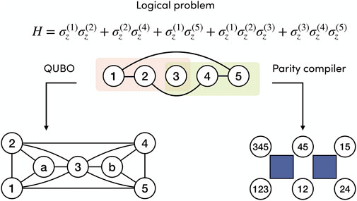
FIGURE 2. Example toy problem H involving high-order interactions that shows how the Parity architecture straightforwardly handles Hamiltonians beyond the QUBO formulation. The problem is represented by the hypergraph at the top of the figure. When decomposed into QUBO form, it requires 7 qubits and 14 two-body interactions, plus additional qubit overhead depending on the embedding. In contrast, the Parity compiler can remap this problem into a 2D grid that requires six qubits with local fields and four-body interactions, represented by the blue squares. No additional embedding is necessary if the hardware is designed for the Parity Architecture.

It is not yet clear what the best Hamiltonian representation is for an optimization problem. The answer will probably depend strongly on the particular use case and will take into account not only the number of qubits needed but also the smoothness of the energy landscape, which has a direct impact on the performance of quantum algorithms (King et al., 2019).

5 Encoding constraints

In this section, we review how to implement the hard constraints associated with the problem, assuming that the encodings of the variables have already been chosen. Hard constraints c(v₁, …, v_N) = K often appear in optimization problems, limiting the search space and making problems even more difficult to solve. We consider polynomial constraints of the form

$\begin{array}{cc}\hfill c\left(v_1,\dots ,v_N\right)=& \sum g_i{v}_i\hfill \\ \hfill & +\sum g_{i,j}{v}_i{v}_j+\sum g_{i,j,k}{v}_i{v}_j{v}_k+\dots ,\hfill \end{array}(36)$

which remain polynomial after replacing the discrete variables v_i with any encoding. The coefficients g_i, g_i,j, … depend on the problem and its constraints. Even if the original problem is unconstrained, the use of sparse encodings such as one-hot or domain wall imposes hard constraints on the quantum variables.

In general, constraints can be implemented dynamically (Hen and Sarandy, 2016; Hen and Spedalieri, 2016) (exploring only quantum states that satisfy the constraints) or as extra terms H_c in the Hamiltonian, such that eigenvectors of H are also eigenvectors of H_c and the ground states of H_c correspond to elements in the domain of f that satisfy the constraint. These can be incorporated as a penalty term H_c into the Hamiltonian that penalizes any state outside the desired subspace:

$H_{\mathrm{c}}=A{\left[c\left(v_1,\dots ,v_N\right)-K\right]}^2,(37)$

or

$H_{\mathrm{c}}=A\left[c\left(v_1,\dots ,v_N\right)-K\right],(38)$

in the special case that c(x₁, …, x_N) ≥ K is satisfied. The constant A must be large enough to ensure that the ground state of the total Hamiltonian satisfies the constraint, but the implementation of large energy scales lowers the efficiency of quantum algorithms (Lanthaler and Lechner, 2021) and additionally imposes a technical challenge. Moreover, extra terms in the Hamiltonian imply additional overhead of computational resources, especially for squared terms such as in Eq. 37. The determination of the optimal energy scale is an important open problem. For some of the problems in the library, we provide an estimation of the energy scales (cf. also Section 8.4.2).

Quantum algorithms for finding the ground state of Hamiltonians, such as QAOA or quantum annealing, require driver terms U_drive = exp(−itH_drive) that spread the initial quantum state to the entire Hilbert space. Dynamical implementation of constraints employs a driver term that only explores the subspace of the Hilbert space that satisfies the constraints. Given an encoded constraint in terms of Ising operators ${\sigma }_z^{(i)}$:

$\begin{array}{cc}\hfill c\left({\sigma }_z^{\left(1\right)},\dots ,{\sigma }_z^{\left(N\right)}\right)=& \sum g_i{\sigma }_z^{\left(i\right)}\hfill \\ \hfill & +\sum g_{i,j}{\sigma }_z^{\left(i\right)}{\sigma }_z^{\left(j\right)}+\cdots =K,\hfill \end{array}(39)$

a driver Hamiltonian H_drive that commutes with $c({\sigma }_z^{(1)},\dots ,{\sigma }_z^{(N)})$ will be restricted to the valid subspace provided the initial quantum state satisfies the constraint:

$\begin{array}{cc}\hfill c|{\psi }_0\rangle & =K|{\psi }_0\rangle \hfill \\ \hfill U_{\text{drive}}c|{\psi }_0\rangle & =U_{\text{drive}}K|{\psi }_0\rangle \hfill \\ \hfill c\left[U_{\text{drive}}|{\psi }_0\rangle \right]& =K\left[U_{\text{drive}}|{\psi }_0\rangle \right].\hfill \end{array}(40)$

In general, the construction of constraint-preserving drivers depends on the problem (Hen and Sarandy, 2016; Hen and Spedalieri, 2016; Hadfield et al., 2017; Chancellor, 2019; Bärtschi and Eidenbenz, 2020; Wang et al., 2020; Fuchs et al., 2021; Bakó et al., 2022). Approximate driver terms have been proposed that admit some degree of leakage and may be easier to construct (Sawaya et al., 2022). Within the Parity Architecture, each term of a polynomial constraint is a single Parity qubit (Lechner et al., 2015; Ender et al., 2023). This implies that for the Parity Architecture the polynomial constraints are simply the conservation of magnetization between the qubits involved:

$\begin{array}{cc}\hfill {\displaystyle \sum _i}{g}_i{\sigma }_z^{\left(i\right)}& +{\displaystyle \sum _{i,j}}{g}_{i,j}{\sigma }_z^{\left(i\right)}{\sigma }_z^{\left(j\right)}+\cdots =K\hfill \\ \hfill & \to \sum _{\mathbf{u}\in c}{g}_{\mathbf{u}}{\sigma }_z^{\left(\mathbf{u}\right)}=K,\hfill \end{array}(41)$

where the Parity qubit ${\sigma }_z^{(\mathbf{u})}$ represents the logical qubits product ${\sigma }_z^{(u_1)}{\sigma }_z^{(u_2)}\dots {\sigma }_z^{(u_n)}$ and we can sum over all these products that appear in the constraint c. A driver Hamiltonian based on exchange (or flip-flop) terms ${\sigma }_{+}^{(\mathbf{u})}{\sigma }_{-}^{(\mathbf{w})}+h.c$., summed over all pairs of products u, w ∈ c, preserves the total magnetization and explores the complete subspace where the constraint is satisfied (Drieb-Schön et al., 2023). The decision tree for encoding constraints is presented in Figure 3.

FIGURE 3

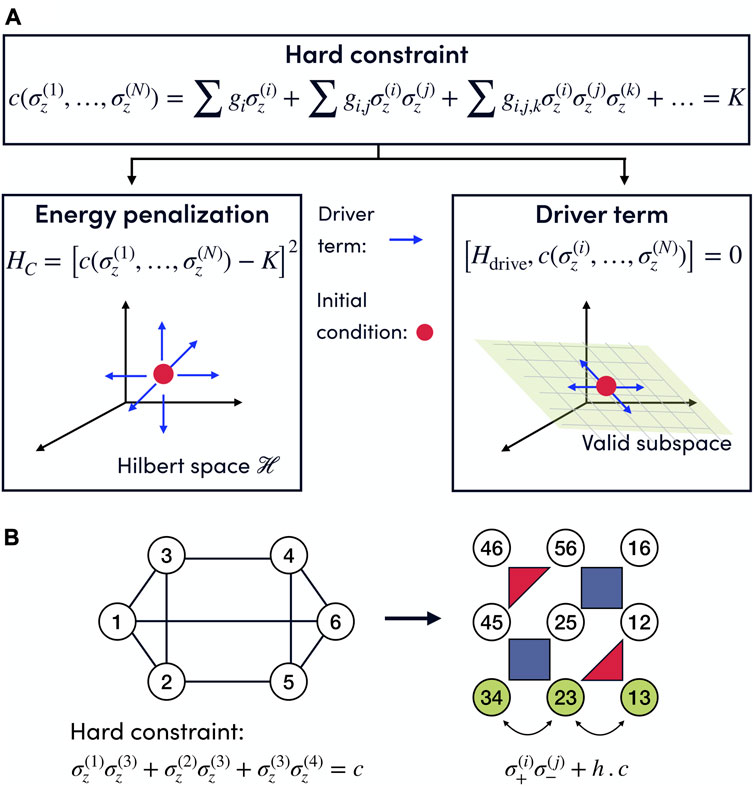
FIGURE 3. (A) Decision tree to encode constraints, which can be implemented as energy penalizations in the problem Hamiltonian or dynamically by selecting a driver Hamiltonian that preserves the desired condition. For energy penalties (left figure), the driver term needs to explore the entire Hilbert space. In contrast, the dynamic implementation of the constraints (right figure) reduces the search space to the subspace satisfying the hard constraint, thus improving the performance of the algorithms. (B) Constrained logical problem (left) and its Parity representation where each term of the polynomial constraint is represented by a single Parity qubit (green qubits), so the polynomial constraints define a subspace in which the total magnetization of the involved qubits is preserved and which can be explored with an exchange driver σ₊σ₋ + h.c. that preserves the total magnetization. Figure originally published in Ref. Drieb-Schön et al. (2023).

6 Use case example

In this section, we present an example of the complete procedure to go from the encoding-independent formulation to the spin Hamiltonian that has to be implemented in the quantum computer, using an instance of the Clustering problem (Section 7.1.1).

Every problem in this library includes a Problem description, indicating the required inputs for defining a problem instance. In the case of the clustering problem, a problem instance is defined from the number of clusters K we want to create, N objects with weights w_i, and distances d_i,j between the objects. Two different types of discrete variables are required, variables v_i = 1, …, K (i = 1, …, N) indicate to which of the K possible clusters the node i is assigned, and variables y_j = 1, …, W_max track the weight in cluster j.

The cost function of the problem only depends on ${\delta }_{v_i}^k$, the value indicators of variables v_i. In this case, ${\delta }_{v_i}^k$ indicates whether the node associated with the discrete variable v_i belongs to the cluster k or not. If two nodes i, j belong to the same cluster k, then the cost function increases by d_i,j, giving the total cost function:

$f={\displaystyle \sum _{k=1}^K}{\displaystyle \sum _{i<j}}{d}_{i,j}{\delta }_{v_i}^k{\delta }_{v_j}^k.(42)$

We can choose any encoding for the variables v_i. For example, if we decide to use binary or Gray encoding, a variable v_i requires D = log₂(K) qubits ${\{x_u^{(i)}\}}_{u=1}^D$(we assume K = 2^D for simplicity, but the resource estimate will not change significantly if this is not the case). From Eq. 12 we see that ${\delta }_{v_i}^k$ is a polynomial of order D in variables $x_u^{(i)}$ with $\left(\genfrac{}{}{0.0pt}{}{D}{j}\right)$ terms of order j and 2^D = K terms in total, so the product ${\delta }_{v_i}^k{\delta }_{v_j}^k$ in the cost function will have 2^D × 2^D = 2^2D = K² terms, with orders between zero and 2D. This product is summed over all the $\frac{N(N-1)}{2}$ pairs i, j, so we can say that $\mathcal{O}(N^2{K}^2)$ terms are required for the cost function. High-order interactions may be prohibitive for some hardware platforms, but if multiqubit gates are available, binary encoding offers an important reduction in the number of qubits.

Alternatively, we can choose a sparse encoding for the variables v_i. Using one-hot encoding, we need K qubits per node, so NK qubits are required for the cost function. The product ${\delta }_{v_i}^k{\delta }_{v_j}^k$ is just a two-qubit interaction $x_k^{(i)}{x}_k^{(j)}$, so the cost function requires $\mathcal{O}(K{N}^2)$ terms. The K qubits associated with a variable v_i must satisfy the core constraint:

$c_i={\displaystyle \sum _{u=1}^K}{x}_u^{\left(i\right)}=1.(43)$

if this constraint is implemented as an energy penalization ${(c_i-1)}^2$, then $\mathcal{O}(K^2)$ terms are added to the spin Hamiltonian for each variable, so $\mathcal{O}(N{K}^2)$ terms in total are associated with the constraint. The advantage of sparse encodings is that low-order interactions are needed for the value indicator functions (in this case, the maximum order is two).

Besides the core constraints associated with the encodings, the clustering problem includes K additional constraints (one per each cluster). The total weight of nodes in any cluster cannot exceed a problem instance specific maximal value W_max:

${\displaystyle \sum _i}{w}_i{\delta }_i^k\le W_{\text{max}},\forall k\in \{1,\dots ,K\}.(44)$

For the kth cluster, this constraint can be expressed in terms of auxiliary variables y_k:

$y_k={\displaystyle \sum _i}{w}_i{\delta }_{v_i}^k.(45)$

Variables y_k are discrete variables in the range 0, …, W_max. Because the value indicators of y_k are not necessary for the constraints, we can use a dense encoding such as binary without dealing with the high-order interactions associated with value indicators of dense encodings. The variables y_k require K log₂(W_max) qubits if we use binary encoding, or KW_max if we use one-hot. These constraints can also be implemented as energy penalizations in the Hamiltonian or can be encoded in the driver term.

The complete procedure for obtaining the spin Hamiltonian is outlined in Figure 4. We emphasize that the optimal encodings and constraint implementations depend on the details of the hardware, such as native gates, connectivity, and the number of qubits. Moreover, the efficiency of quantum algorithms is also related to the smoothness of the energy landscape, and some encodings can provide better results even though they require more qubits (see, for example, Tamura et al., 2021).

FIGURE 4

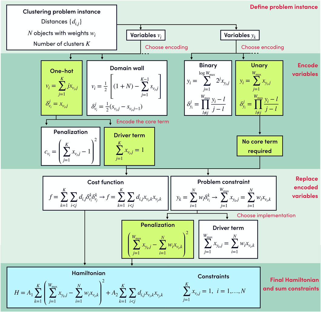
FIGURE 4. Example decision tree for the clustering problem. The entire process is presented in four different blocks and the decisions taken are highlighted in green. The formulation of a problem instance requires the discrete variables v_i and y_k to be encoded in terms of qubit operators. In this example, the v_i variables are encoded using the one-hot encoding while for the y_k variables we use the binary encoding. The Hamiltonian is obtained by substituting in the encoding-independent expressions of Eqs 48, 50 the discrete variables v_i, y_k and the value indicators ${\delta }_v^{\alpha }$ according to the chosen encoding. Core terms associated with sparse encodings (one-hot in this case) and the problem constraints can be added to the Hamiltonian as energy penalizations or implemented dynamically in the driver term of the quantum algorithm as sum constraints.

7 Problem library

The problems included in the library are classified into four categories: subsets, partitions, permutations, and continuous variables. These categories are defined by the role of the discrete variable and are intended to organize the library and make it easier to find problems but also to serve as a basis for the formulation of similar use cases. An additional category in Section 7.5 contains problems that do not fit into the previous categories but may also be important use cases for quantum algorithms. In Section 8 we include a summary of recurrent encoding-independent building blocks that are used throughout the library and could be useful in formulating new problems.

7.1 Partitioning problems

The goal of partitioning problems is to look for partitions of a set U, minimizing a cost function f. A partition P of U is a set $P:={\left\{U_k\right\}}_{k\in K}$ of subsets U_k ⊂ U, such that $U={\bigcup }_{k=1}^K{U}_k$ and U_k ∩ U_k′ = 0 if k ≠ k′. Partitioning problems require a discrete variable v_i for each element u_i ∈ U. The value of v_i indicates to which subset the element belongs, so v_i can take K different values. Values assigned to the subsets are arbitrary, therefore the value of v_i is usually not important in these cases, but only the value indicator ${\delta }_{v_i}^{\alpha }$ is needed, so sparse encodings may be convenient for these variables.

7.1.1 Clustering problem

a. Description Let $U={\left\{u_i\right\}}_{i=1}^N$ be a set of N elements, characterized by weights w_i ∈ {1, …, w_max} and distances d_i,j between them. The clustering problem looks for a partition of the set U into K non-empty subsets U_k that minimizes the distance between vertices in each subset. Partitions are subject to a weight restriction: for every subset U_k, the sum of the weights of the vertices in the subset must not exceed a given maximum weight W_max.

b. Variables We can define a variable v_i = 1, …, K for each element in U. We also require an auxiliary variable y_j = 0, 1, …, W_max per subset U_k, that indicates the total weight of the elements in U_k:

$y_k={\displaystyle \sum _{\left\{i:u_i\in U_k\right\}}}{w}_i.(46)$

c. Constraints The weight restriction is an inequality constraint:

$y_k\le W_{\text{max}},(47)$

which can be expressed as:

$y_k={\displaystyle \sum _i}{w}_i{\delta }_{v_i}^k.(48)$

if the encoding for the auxiliary variables makes it necessary (e.g., a binary encoding and W_max not a power of 2), this constraint must be shifted as is described in Section 8.2.3.

d. Cost function The sum of the distances of the elements of a subset is:

$f_k={\displaystyle \sum _{\left\{i<j:u_i,u_j\in U_k\right\}}}{d}_{i,j}={\displaystyle \sum _{i<j}}{d}_{i,j}{\delta }_{v_i}^k{\delta }_{v_j}^k,(49)$

and the cost function results:

$f={\displaystyle \sum _k}{f}_k.(50)$

e. References Studied by Feld et al. (2019) as part of the Capacitated Vehicle Routing problem.

7.1.2 Number partitioning

a. Description Given a set U of N real numbers u_i, we can look for a partition of size K such that the sum of the numbers in each subset is as homogeneous as possible.

b. Variables The problem requires N variables v_i ∈ [1, K], one per element u_i. The value of v_i indicates to which subset u_i belongs.

c. Cost function The partial sums can be represented using the value indicators associated with the variables v_j:

$p_j={\displaystyle \sum _{u_i\in U_j}}{u}_i={\displaystyle \sum _{i=1}^N}{u}_i{\delta }_{v_i}^j.(51)$

there are three common approaches for finding the optimal partition: maximizing the minimum partial sum, minimizing the largest partial sum, or minimizing the difference between the maximum and the minimum partitions. The latter option can be formulated as

$f={\displaystyle \sum _{i<j}}{\left(p_i-p_j\right)}^2.(52)$

In order to minimize the maximum partial sum (maximizing the minimum partial sum is done analogously) we can introduce an auxiliary variable l that can take values 1, …, ∑_iu_i ≡ l_max. Depending on the problem instance the range of l can be restricted further. The first term in the cost function

$f=l_{\text{max}}\left(1-{\displaystyle \prod _i}\mathrm{\Theta }\left(l-p_i\right)\right)+l(53)$

then enforces that l is as least as large as the maximum p_i (Section 8.1.3) and the second term minimizes l. The theta step function can be expressed in terms of the value indicator functions according to the building block Eq. 144 by either introducing auxiliary variables or expressing the value indicators directly according to the discussion in Section 8.4.1.

d. Special cases For K = 2, the cost function that minimizes the difference between the partial sums is

$\begin{array}{cc}\hfill f& ={\left(p_2-p_1\right)}^2\hfill \\ \hfill & ={\left[{\displaystyle \sum _{i=1}^N}\left({\delta }_{v_i}^1-{\delta }_{v_i}^2\right)u_i\right]}^2.\hfill \end{array}(54)$

The only two possible outcomes for ${\delta }_{v_i}^1-{\delta }_{v_i}^2$ are ±1, so these factors can be trivially encoded using spin variables s_i = ±1, leading to

$f={\displaystyle \sum _{i=1}^N}{s}_i{u}_i.(55)$

e. References The Hamiltonian formulation for K = 2 can be found in Lucas (2014).

7.1.3 Graph coloring

a. Description The nodes of the graph G = (V, E) are divided into K different subsets, each one representing a different color. We can look for a partition in which two adjacent nodes are painted with different colors and which minimizes the number of colors used.

b. Variables We define a variable v_i = 1…K for each node i = 1, …, N in the graph.

c. Constraints We must penalize solutions for which two adjacent nodes are painted with the same color. The cost function of the graph partitioning problem presented in Eq. 61 can be used for the constraint of graph coloring. In that case, $\left[1-\delta (v_i-v_j)\right]A_{i,j}$ was used to count the number of adjacent nodes belonging to different subsets, now we can use δ(v_i − v_j)A_i,j to indicate if nodes i and j are painted with the same color. Therefore the constraint is (see building block Section 8.2.1)

$c={\displaystyle \sum _{i<j}}\delta \left(v_i-v_j\right)A_{i,j}=0.(56)$

d. Cost function The decision problem (“Is there a coloring that uses K colors?”) can be answered by implementing the constraint as a Hamiltonian H = c (note that c ≥ 0). The existence of a solution with zero energy implies that a coloring with K colors exists.

Alternatively we can look for the coloring that uses the minimum number of colors. To check if a color α is used, we can use the following term (see building block Section 8.2.2):

$u_{\alpha }=1-{\displaystyle \prod _{i=1}^N}\left(1-{\delta }_{v_i}^{\alpha }\right),(57)$

which is one if and only if color α is not used in the coloring, and 0 if at least one node is painted with color α. The number of colors used in the coloring is the cost function of the problem:

$f={\displaystyle \sum _{\alpha =1}^K}{u}_{\alpha }.(58)$

This objective function can be very expensive to implement since u_α includes products of ${\delta }_{v_i}^{\alpha }$ of order N, so a good estimation of the minimum number K_min would be useful to avoid using an unnecessarily large K.

e. References The one-hot encoded version of this problem can be found in Lucas (2014).

7.1.4 Graph partitioning

a. Description Graph partitioning divides the nodes of a graph G = (V, E) into K different subsets, so that the number of edges connecting nodes in different subsets (cut edges) is minimized or maximized.

b. Variables We can use one discrete variable v_k = 1, …, K per node in the graph, which indicates to which partition the node belongs.

c. Cost function An edge connecting two nodes i and j is cut when v_i ≠ v_j. It is convenient to use the symbol (see building block Section 8.1.4):

$\delta \left(v_i-v_j\right)={\displaystyle \sum _{\alpha =1}^K}{\delta }_{v_i}^{\alpha }{\delta }_{v_j}^{\alpha }=\left\{\begin{array}{c}1\mathrm{i}\mathrm{f}{v}_i=v_j\hfill \\ 0\mathrm{i}\mathrm{f}{v}_i\ne v_j\hfill \end{array}\right.,(59)$

which is equal to 1 when nodes i and j belong to the same partition (v_i = v_j) and zero when not (v_i ≠ v_j). In this way, the term:

$\left(1-\delta \left(v_i-v_j\right)\right)A_{i,j}(60)$

is equal to 1 if there is a cut edge connecting nodes i and j, being A_i,j the adjacency matrix of the graph. The cost function for minimizing the number of cut edges is obtained by summing over all the nodes:

$f={\displaystyle \sum _{i<j}}\left[1-\delta \left(v_i-v_j\right)\right]A_{i,j},(61)$

or alternatively −f to maximize the number of cut edges.

d. Constraints A common constraint imposes that partitions have a specific size. The element counting building block Section 8.1.1 is defined as

$t_{\alpha }={\displaystyle \sum _{i=1}^{|V|}}{\delta }_{v_i}^{\alpha }.(62)$

If we want the partition α to have L elements, then

$t_{\alpha }=L(63)$

must hold. If we want the two partitions, α and β, to have the same size, then the constraint is

$t_{\alpha }=t_{\beta },(64)$

and all the partitions will have the same size, imposing

${\displaystyle \sum _{a<b}}{\left(t_a-t_b\right)}^2=0(65)$

which is only possible if |V|/K is a natural number.

e. References The Hamiltonian for K = 2 can be found in Lucas (2014).

f. Hypergraph partitioning The problem formulation can be extended to hypergraphs. A hyperedge is cut when it contains vertices from at least two different subsets. Given a hyperedge e of G, the function

$\mathrm{c}\mathrm{u}\mathrm{t}\left(e\right)={\displaystyle \prod _{i,j\in e}}\delta \left(v_i-v_j\right)(66)$

is only equal to 1 if all the vertices included in e belong to the same partition, and zero in any other case. The product over the vertices i, j of the edge e only needs to involve pairs such that every vertex appears at least once. The optimization objective of minimizing the cut hyperedges is implemented by the sum of penalties

$\begin{array}{cc}\hfill f& ={\displaystyle \sum _{e\in E}}\left(1-\mathrm{c}\mathrm{u}\mathrm{t}\left(e\right)\right)\hfill \\ \hfill & ={\displaystyle \sum _{e\in E}}\left(1-{\displaystyle \prod _{i,j\in e}}{\displaystyle \sum _{a=1}^K}{\delta }_i^a{\delta }_j^a\right).\hfill \end{array}(67)$

This objective function penalizes all possible cuts in the same way, regardless of the number of vertices cut or the number of partitions to which an edge belongs.

7.1.5 Clique cover

a. Description Given a graph G = (V, E), we seek the minimum number of colors K for coloring all vertices such that the subsets W_α of vertices with the color α together with the edge set E_α restricted to edges between vertices in W_α form complete graphs. A subproblem is to decide if there is a clique cover using K colors.

b. Variables For each vertex i = 1, …, N we define variables v_i = 1, …, K indicating the color that vertex is assigned to. If the number of colors is not given, one has to start with an initial guess or a minimal value for K.

c. Constraints In this problem, G_α = (W_α, E_α) has to be a complete graph, so the maximum number of edges in E_α must be present. Using the element counting building block, we can calculate the number of vertices with color α (see bulding block Section 8.1.1):

$t_{\alpha }={\displaystyle \sum _{i=1}^N}{\delta }_i^{\alpha }.(68)$

if G_α is a complete graph, then the number of edges in E_α is t_α(t_α − 1)/2 and thus the constraint reads

$c={\displaystyle \sum _{\alpha =1}^K}\left(\frac{t_{\alpha }\left(t_{\alpha }-1\right)}{2}-{\displaystyle \sum _{\left(i,j\right)\in E}}{\delta }_i^{\alpha }{\delta }_j^{\alpha }\right)=0.(69)$

Note that we do not have to square the term as it can never be negative.

d. Cost function The decision problem (“Is there a clique cover using K colors?”) can be answered using the constraint c as the Hamiltonian of the problem. For finding the minimum number of colors K_min for which a clique cover exists (the clique cover number), we can add a cost function for minimizing K. As in the graph coloring problem, we can minimize the number of colors using

$f={\displaystyle \sum _{\alpha }}\left(1-u_{\alpha }\right),(70)$

where

$u_{\alpha }={\displaystyle \prod _{i=1}^N}\left(1-{\delta }_{v_i}^{\alpha }\right)(71)$

indicates if the color α is used or not (see building block Section 8.2.2).

e. References The one-hot encoded Hamiltonian of the decision problem can be found in Lucas (2014).

7.2 Constrained subset problems

Given a set U, we look for a non-empty subset U₀ ⊆ U that minimizes a cost function f while satisfying a set of constraints c_i. In general, these problems require a binary variable x_i per element in U which indicates if the element i is included or not in the subset U₀. Although binary variables are trivially encoded in single qubits, non-binary auxiliary variables may be necessary to formulate constraints, so the encoding-independent formulation of these problems is still useful.

7.2.1 Cliques

a. Description A clique on a given graph G = (V, E) is a subset of vertices W ⊆ V such that W and the subset E_W of edges between vertices in W is a complete graph, i.e., the maximal possible number of edges in E_W is present. The goal is to find a clique with cardinality K. Additionally, one could ask what the largest clique of the graph is.

b. Variables We can define |V| binary variables x_i that indicate whether vertex i is in the clique or not.

c. Constraints This problem has two constraints, namely, that the cardinality of the clique is K and that the clique indeed has the maximum number of edges. The former is enforced by

$c_1={\displaystyle \sum _{i=1}^{|V|}}{x}_i=K(72)$

and the latter by

$c_2={\displaystyle \sum _{\left(i,j\right)\in E}}{x}_i{x}_j=\frac{K\left(K-1\right)}{2}.(73)$

If constraints are implemented as energy penalization, one has to ensure that the first constraint is not violated to decrease the penalty for the second constraint. Using the cost/gain analysis (Section 8.4.2) of a single spin flip this is prevented as long as a₁⪆a₂Δ, where Δ is the maximal degree of G and a_1,2 are the energy scales of the first and second constraints.

d. Cost function The decision problem (“Is there a clique of size K?”) can be solved using the constraints as the Hamiltonian of the problem. If we want to find the largest clique of the graph G, we must encode K as a discrete variable, K = 1, …, K_max, where K_max = Δ is the maximum degree of G and the largest possible size of a clique. The cost function for this case is simply the value of K:

$f=-K(74)$

e. Resources Implementing constraints as energy penalizations, the total cost function for the decision problem (fixed K),

$f={\left(c_1-K\right)}^2+{\left(c_2-\frac{K\left(K-1\right)}{2}\right)}^2,(75)$

has interaction terms with maximum order of two and the number of terms scales with |E| + |V|². If K is encoded as a discrete variable, the resources depend on the chosen encoding.

f. References This Hamiltonian was formulated in Lucas (2014) using one-hot encoding.

7.2.2 Maximal independent set

a. Description Given a hypergraph G = (V, E) we look for a subset of vertices S ⊂ V such that there are no edges in E connecting any two vertices of S. Finding the largest possible S is an NP-hard problem.

b. Variables We use a binary variable x_i for each vertex in V.

c. Cost function For maximizing the number of vertices in S, the cost function is

$f=-{\displaystyle \sum _{i=1}^{|V|}}{x}_i.(76)$

d. Constraints Given two elements in S, there must not be any edge of hyperedge in E connecting them. The constraint

$c={\displaystyle \sum _{i,j\in V}}{A}_{i,j}{x}_i{x}_j(77)$

counts the number of adjacent vertices in S, with A as the adjacency matrix. By setting c = 0, the vertices in S form an independent set.

e. References   See Lucas (2014) and Choi (2010) for graphs.

7.2.3 Set packing

a. Description Given a set U and a family $S={\{V_i\}}_{i=1}^N$ of subsets V_i of U, we want to find set packings, i.e., subsets of S such that all subsets are pairwise disjoint, V_i ∩ V_j = ∅. Finding the maximum packing (the maximum number of subsets V_i) is the NP-hard optimization problem called set packing.

b. Variables We define N binary variables x_i that indicate whether subset V_i belongs to the packing.

c. Cost function Maximizing the number of subsets in the packing is achieved with the element counting building block

$f=-{\displaystyle \sum _{i=1}^N}{x}_i.(78)$

d. Constraints In order to ensure that any two subsets of the packings are disjoint we can impose a cost on overlapping sets with

$c={\displaystyle \sum _{i,j:V_i\cap V_j\ne \varnothing }}{x}_i{x}_j=0.(79)$

e. Resources The total cost function H = H_A + H_B has interaction terms with maximum order of two (so it is a QUBO problem) and the number of terms scales up to N².

f. References This problem can be found in Lucas (2014).

7.2.4 Vertex cover

a. Description Given a hypergraph G = (V, E) we want to find the smallest subset C ⊆ V such that all edges contain at least one vertex in C.

b. Variables We define |V| binary variables x_i that indicate whether vertex i belongs to the cover C.

c. Cost function Minimizing the number of vertices in C is achieved with the element counting building block

$f={\displaystyle \sum _{i=1}^{|V|}}{x}_i.(80)$

d. Constraints With

$c={\displaystyle \sum _{e=\left(u_1,\dots ,u_k\right)\in E}}{\displaystyle \prod _{a=1}^k}\left(1-x_{u_a}\right)=0(81)$

one can penalize all edges that do not contain vertices belonging to C. Encoding the constraint as an energy penalization, the Hamiltonian results in

$H=Af+Bc.(82)$

by setting B > A we can avoid the constraint being traded off against the minimization of C.

e. Resources The maximum order of the interaction terms is the maximum rank of the hyperedges k and the number of terms scales with |E|2^k + |V|.

f. References The special case that only considers graphs can be found in Lucas (2014).

7.2.5 Minimal maximal matching

a. Description Given a hypergraph G = (V, E) with edges of maximal rank k we want to find a minimal (i.e., fewest edges) matching C ⊆ E which is maximal in the sense that all edges with vertices that are not incident to edges in C have to be included in the matching.

b. Variables We define |E| binary variables x_i that indicate whether an edge belongs to the matching C.

c. Cost function Minimizing the number of edges in the matching is simply done by the cost function

$f_A=A{\displaystyle \sum _{i=1}^{|E|}}{x}_i.(83)$

d. Constraints We have to enforce that C is indeed a matching, i.e., that no two edges which share a vertex belong to C. Using an energy penalty, this is achieved by:

$f_B=B{\displaystyle \sum _{v\in V}}{\displaystyle \sum _{\left(i,j\right)\in \partial v}}{x}_i{x}_j=0,(84)$

where ∂v is the set of edges connected to vertex v. Additionally, the matching should be maximal. For each vertex u, we define a variable y_u = ∑_i∈∂ux_i which is only zero if the vertex does not belong to an edge of C. If the first constraint is satisfied, this variable can only be 0 or 1. In this case, the constraint can be enforced by

$f_C=C{\displaystyle \sum _{e=\left(u_1,\dots ,u_k\right)\in E}}{\displaystyle \prod _{a=1}^k}\left(1-y_{u_a}\right)=0.(85)$

However, one has to make sure that the constraint implemented by f_B is not violated in favor of f_C which could happen if for some v, y_v > 1 and for m neighboring vertices y_u = 0. Then the contributions from v are given by

$f_v=B{y}_v\left(y_v-1\right)\frac{1}{2}+C\left(1-y_v\right)m(86)$

and since m + y_v is bounded by the maximum degree Δ of G times the maximum rank of the hyperedges k, we need to set B > (Δk − 2)C to ensure that the ground state of f_B + f_C does not violate the first constraint. Finally, one has to prevent f_C being violated in favor of f_A which entails C > A.

e. Resources The maximum order of the interaction terms is k and the number of terms scales roughly with (|V| + |E|2^k)Δ(Δ − 1).

f. References This problem can be found in Lucas (2014).

7.2.6 Set cover

a. Description Given a set $U={\{u_{\alpha }\}}_{\alpha =1}^n$ and N subsets V_i ⊆ U, we look for the minimum number of V_i such that U = ⋃V_i.

b. Variables We define a binary variable x_i = 0, 1 for each subset V_i that indicates if the subset V_i is selected or not. We also define auxiliary variables y_α = 1, 2, …, N that indicate how many active subsets (V_i such that x_i = 1) contain the element u_α.

c. Cost function The cost function is simply

$f={\displaystyle \sum _{i=1}^N}{x}_i,(87)$

which counts the number of selected subsets V_i.

d. Constraints The constraint $U={\bigcup }_{i:x_i=1}{V}_i$ can be expressed as

$y_{\alpha }>0,\forall \alpha =1,\dots ,n,(88)$

which implies that every element u_α ∈ U is included at least once. These inequalities are satisfied if y_α are restricted to the valid values (y_α = 1, 2, …, N, y_α ≠ 0) (Section 8.2.3). The values of y_α should be consistent with those of x_i, so the constraint is

$c_{\alpha }=y_{\alpha }-{\displaystyle \sum _{i:u_{\alpha \in V_i}}}{x}_i=0.(89)$

e. Special case: exact cover If we want each element of U to appear once and only once on the cover, then y_α = 1, for all α and the constraint of the problem reduces to

$c_{\alpha }={\displaystyle \sum _{i:\alpha \in V_i}}{x}_i=1.(90)$

f. References The one-hot encoded Hamiltonian can be found in Lucas (2014).

7.2.7 Knapsack

a. Description A set U contains N objects, each of them with a value d_i and a weight w_i. We look for a subset of U with the maximum value ∑d_i such that the total weight of the selected objects does not exceed the upper limit W.

b. Variables We define a binary variable x_i = 0, 1 for each element in U that indicates if the element i is selected or not. We also define an auxiliary variable y that indicates the total weight of the selected objects:

$y={\displaystyle \sum _{i:x_i=1}}{w}_i.(91)$

if the weights are natural numbers $w_i\in \mathbb{N}$ then y is also natural, and the encoding of this auxiliary variable is greatly simplified.

c. Cost function The cost function is given by

$f=-{\displaystyle \sum _{i=1}^N}{d}_i{x}_i,(92)$

which counts the value of the selected elements.

d. Constraints The constraint y < W is implemented by forcing y to take one of the possible values y = 1, …W − 1 (see Section 8.2.3). The value of y must be consistent with the selected items from U:

$c=y-{\displaystyle \sum _i^N}{w}_i{x}_i=0.(93)$

e. References The one-hot encoded Hamiltonian can be found in Lucas (2014).

7.3 Permutation problems

In permutation problems, we need to find a permutation of N elements that minimizes a cost function while satisfying a given set of constraints. In general, we will use a discrete variable v_i ∈ [1, N] that indicates the position of the element i in the permutation.

7.3.1 Hamiltonian cycles

a. Description For a graph G = (V, E), we ask if a Hamiltonian cycle, i.e., a closed path that connects all nodes in the graph through the existing edges without visiting the same node twice, exists.

b. Variables We define a variable v_i = 1, …, |V| for each node in the graph, that indicates the position of the node in the permutation.

c. Cost function For this problem, there is no cost function, so every permutation that satisfies the constraints is a solution to the problem.

d. Constraints This problem requires two constraints. The first constraint is inherent to all permutation problems and imposes the |V| variables {v_i} to be a permutation of [1, …, |V|]. This is equivalent to requiring v_i ≠ v_j if i ≠ j, which can be encoded with the following constraint (Section 8.2.1):

$c_1={\displaystyle \sum _{\alpha =1}^N}{\displaystyle \sum _{i\ne k}}{\delta }_{v_i}^{\alpha }{\delta }_{v_k}^{\alpha }=0.(94)$

The second constraint ensures that the path only goes through the edges of the graph. Let A be the adjacency matrix of the graph, such that A_i,j = 1 if there is an edge connecting nodes i and j and zero otherwise. To penalize invalid solutions, we use the constraint

$c_2={\displaystyle \sum _{i,j}}{\displaystyle \sum _{\alpha =1}^{|V|}}\left(1-A_{i,j}\right)\left({\delta }_{v_i}^{\alpha }{\delta }_{v_j}^{\alpha +1}+{\delta }_{v_i}^{\alpha +1}{\delta }_{v_j}^{\alpha }\right)=0,(95)$

which counts how many adjacent nodes in the solution are not connected by an edge in the graph. α = |V| + 1 represents α = 1 since we are looking for a closed path.

e. References The one-hot encoded Hamiltonian can be found in Lucas (2014).

7.3.2 Traveling salesperson problem (TSP)

a. Description The TSP is a trivial extension of the Hamiltonian cycles problem. In this case, the nodes represent cities and the edges are the possible roads connecting the cities, although in general it is assumed that all cities are connected (the graph is complete). For each edge connecting cities i and j there is a cost w_i,j. The solution of the TSP is the Hamiltonian cycle that minimizes the total cost ∑w_i,j.

b. Variables We define a variable v_i = 1, …, |V| for each node in the graph, indicating the position of the node in the permutation.

c. Cost function If the traveler goes from city i at position α to city j in the next step, then

${\delta }_{v_i}^{\alpha }{\delta }_{v_j}^{\alpha +1}=1,(96)$

otherwise, that expression would be zero. Therefore the total cost of the travel is codified in the function:

$f={\displaystyle \sum _{\alpha }}{\displaystyle \sum _{i<j}}{w}_{i,j}\left({\delta }_{v_i}^{\alpha }{\delta }_{v_j}^{\alpha +1}+{\delta }_{v_j}^{\alpha }{\delta }_{v_i}^{\alpha +1}\right).(97)$

as for Hamiltonian cycles, α = |V| + 1 represents α = 1 since we are looking for a closed path.

d. Constraints The constraints are the same as those used in the Hamiltonian cycles problem (see paragraph 7.3.1). If the graph is complete (all the cities are connected) then constraint c₂ is not necessary.

e. References The one-hot encoded Hamiltonian can be found in Lucas (2014).

7.3.3 Machine scheduling

a. Description Machine scheduling problems seek the best way to distribute a number of jobs over a finite number of machines. These problems explore permutations of the job list, where the position of a job in the permutation indicates on which machine and at what time the job is executed. Many variants of the problem exist, including formulations in terms of spin Hamiltonians (Venturelli et al., 2015; Kurowski et al., 2020; Amaro et al., 2022). Here we consider the problem of M machines and N jobs, where all jobs take the same amount of time to complete, so the time can be divided into time slots of equal duration t. It is possible to include jobs of duration nt $(n\in \mathbb{N})$ by using appropriate constraints that force some jobs to run in consecutive time slots on the same machine. In this way, problems with jobs of different duration can be solved by choosing a sufficiently short time t.

b. Variables We define variables v_m,t = 0, …N, where the subindex m = 1, …M indicates the machine and t = 1, …T the time slot. When v_m,t = 0, the machine m is unoccupied in time slot t, and if v_m,t = j ≠ 0 then the job j is done in the machine m, in the time slot t.

c. Constraints There are many possible constraints depending on the use case we want to run. As in every permutation problem, we require that no pair of variables have the same value, v_m,t ≠ v_m′,t′, otherwise, some jobs would be performed twice. We also require each job to be complete so there must be exactly one v_m,t = j for each job j. This constraint is explained in Section 8.2.1 and holds for every job j ≠ 0:

$c_1={\displaystyle \sum _{j\ne 0}}{\left[{\displaystyle \sum _{m,t}}{\delta }_{v_{m,t}}^j-1\right]}^2=0.(98)$

Note that if job j is not assigned (i.e., there are no m, t such that v_m,t = j) then c₁ > 0. Also, if there is more than one variable v_m,t = j, then again c₁ > 0. The constraint will be satisfied (c₁ = 0) if and only if every job is assigned to a single time slot on a single machine.

Suppose job k can only be started if another job, j, has been done previously. This constraint can be implemented as

$c_{2,k>j}={\displaystyle \sum _{m,m^{\prime },t\ge t^{\prime }}}{\delta }_{v_{m,t}}^j{\delta }_{v_{m^{\prime },t^{\prime }}}^k=0,(99)$

which precludes any solution in which job j is done after job k. Alternatively, it can be codified as

$c_{2,k>j}^{\prime }={\displaystyle \sum _{m,m^{\prime },t<t^{\prime }}}{\delta }_{v_{m,t}}^j{\delta }_{v_{m^{\prime },t^{\prime }}}^k=1.(100)$

These constraints can be used to encode problems that consider jobs with different operations O₁, …O_q that must be performed in sequential order. Note that constraints $c_2,c_2^{\prime }$ allow the use of different machines for different operations. If we want job k to be done immediately after work j, we can substitute t′ by t + 1 in $c_2^{\prime }$.

If we want two jobs j₁ and j₂ to run on the same machine in consecutive time slots, the constraint can be encoded as

$c_3={\displaystyle \sum _{m,t}}{\delta }_{v_{m,t}}^{j_1}{\delta }_{v_{m,t+1}}^{j_2}=1,(101)$

or as a reward term in the Hamiltonian,

$c_3^{\prime }=-{\displaystyle \sum _{m,t}}{\delta }_{v_{m,t}}^{j_1}{\delta }_{v_{m,t+1}}^{j_2},(102)$

that reduces the energy of any solution in which job j₂ is performed immediately after job j₁ on the same machine m. This constraint allows the encoding of problems with different job durations since j₁ and j₂ can be considered part of the same job of duration 2t.

d. Cost function Different objective functions can be chosen for this problem, such as minimizing machine idle time or early and late deliveries. A common option is to minimize the makespan, i.e., the time slot of the last scheduled job. To do this, we first introduce an auxiliary function $\tau \left(v_{m,t}\right)$ that indicates the time slots in which a job has been scheduled:

$\tau \left(v_{m,t}\right)=\left\{\begin{array}{cc}t\hfill & \mathrm{i}\mathrm{f}{v}_{m,t}\ne 0\hfill \\ 0\hfill & \mathrm{i}\mathrm{f}{v}_{m,t}=0.\hfill \end{array}\right.(103)$

These functions can be generated from v_m,t:

$\tau \left(v_{m,t}\right)=\left(1-{\delta }_{v_{m,t}}^0\right).(104)$

Note that the maximum value of τ corresponds to the makespan of the problem, which is to be minimized. To do this, we introduce the extra variable τ_max and penalize configurations where τ_max < τ(v_m,t) for all m, t:

$f_{{\tau }_{\text{max}}}={\displaystyle \prod _{m,t}}\mathrm{\Theta }\left[\tau \left(v_{m,t}\right)-{\tau }_{\text{max}}\right],(105)$

with

$\mathrm{\Theta }\left(x\right)=\left\{\begin{array}{c}1\mathrm{i}\mathrm{f}x\ge 0\hfill \\ 0\mathrm{i}\mathrm{f}x<0.\hfill \end{array}\right.(106)$

For details on how Θ(x) can be expressed see Section 8.1.2. By minimizing $f_{{\tau }_{\text{max}}}$, we ensure that τ_max ≥ τ(v_m,t). Then, the cost function is used to simply minimize τ_max, the latest time a job can be scheduled, via

$f={\tau }_{\text{max}}.(107)$

An alternative cost function for this problem is

$f^{\prime }={\displaystyle \sum _{m,t}}\tau \left(v_{m,t}\right),(108)$

which forces all jobs to be scheduled as early as possible.

e. References Quantum formulations of this and related problems can be found in Refs. Venturelli et al. (2015); Kurowski et al. (2020); Amaro et al. (2022) and Carugno et al. (2022).

7.3.4 Nurse scheduling problem

a. Description In this problem we have N nurses and D working shifts. Nurses must be scheduled with minimal workload following hard and soft constraints, such as minimum workload n_min,t of nurses i (where nurse i contributes workload p_i) in a given shift t, and balancing the number of shifts to be as equal as possible. Furthermore, no nurse should have to work on more than d_max consecutive days.

b. Variables We define ND binary variables v_i,t indicating whether nurse i is scheduled for shift t.

c. Cost function The cost function, whose minimum corresponds to the minimal number of overall shifts, is given by

$f={\displaystyle \sum _{t=1}^D}{\displaystyle \sum _{i=1}^N}{v}_{i,t}(109)$

d. Constraints Balancing of the shifts is expressed by the constraint

$c={\displaystyle \sum _{i<j}}{\left({\displaystyle \sum _t}{v}_{i,t}-{\displaystyle \sum _{t^{\prime }}}{v}_{j,t^{\prime }}\right)}^2.(110)$

In order to get a minimal workload per shift we introduce the auxiliary variables y_t which we bind to the values

$y_t={\displaystyle \sum _{i=1}^N}{p}_i{v}_{i,t}(111)$

with the penalty terms

${\left(y_t-{\displaystyle \sum _{i=1}^N}{p}_i{v}_{i,t}\right)}^2.(112)$

Now the constraint takes the form

$c={\displaystyle \sum _{t=1}^D}{\displaystyle \sum _{\alpha <n_{\text{min},t}}}{\delta }_{y_t}^{\alpha }=0.(113)$

Note that we can also combine the cost function for minimizing the number of shifts and this constraint by using the cost function

$f={\displaystyle \sum _{t=1}^D}{\left({\displaystyle \sum _{i=1}^N}{p}_i{v}_{i,t}-n_{\text{min},t}\right)}^2.(114)$

Finally, the constraint that a nurse i should work in maximally d_max consecutive shifts reads

$c\left(i\right)={\displaystyle \sum _{t_1-t_2>d_{\text{max}}}}{\displaystyle \prod _{t^{\prime }=t_1}^{t_2}}{v}_{i,t^{\prime }}=0.(115)$

e. References This problem can be found in Ikeda et al. (2019).

7.4 Real variables problems

Some problems are defined by a set of real variables $\{v_i\in \mathbb{R},i=1,\dots ,d\},$ and a cost function f(v_i) that has to be minimized. We again want to express these problems as Hamiltonians whose ground state represents an optimal solution. This involves three steps. First, encode the continuous variables into discrete ones. Second, choose an encoding of these discrete variables to spin variables exactly as before, and third, a decoding step is necessary that maps the solution to our discrete problem back to the continuous domain. In the following, we investigate two possible methods one could use for the first step.

a. Standard discretization Given a vector $v\in {\mathbb{R}}^d$ one could simply discretize it by partitioning the axis into intervals with the length of the aspired precision q, i.e., the components of v = (v_i), i = 1, …, d are mapped to $v_i\to {\tilde{v}}_i\in \mathbb{N}$ such that $({\tilde{v}}_i-1)q\le v_i<{\tilde{v}}_{i}q$.

Depending on the problem it might also be useful to have different resolutions for different axes or a non-uniform discretization, e.g., logarithmic scaling of the interval length.

For the discrete variables ${\tilde{v}}_i$ one can use the encodings in Section 3. In the final step after an intermediate solution,${\tilde{v}}^{*}$, is found, one has to map it back to ${\mathbb{R}}^d$ by uniformly sampling the components of v* from the hypercuboids corresponding to ${\tilde{v}}^{*}$. Any intermediate solution that is valid for the discrete encoding can also be decoded and thus there are no core terms in the cost function besides those from the discrete encoding.

b. Random subspace coding A further possibility to encode a vector $v\in {\mathbb{R}}^d$ into discrete variables is random subspace coding (Rachkovskii et al., 2005). One starts by randomly choosing a set of coordinates $D_n:=\left\{\mathrm{1,2},\dots ,d_n\right\}\subset \left\{\mathrm{1,2},\dots ,d\right\}$. For each i ∈ D_n, a Dirichlet process is used to pick an interval [a_i, b_i] in the i-coordinate direction in ${\mathbb{R}}^d$ (Devroye et al., 1993). We denote

$\begin{array}{cc}\hfill {\pi }_i:{\mathbb{R}}^d& \to \mathbb{R}\hfill \\ \hfill x=\left(x_1,\dots ,x_d\right)& \mapsto {\pi }_i\left(x\right):=x_i\hfill \end{array}(116)$

for the projection to the ith coordinate. A hyperrectangle $R\subset {\mathbb{R}}^d$ is defined as

$R:=\left\{x\in {\mathbb{R}}^d|{\pi }_i\left(x\right)\in \left[a_i,b_i\right],\forall i\in D_n\right\}.(117)$

For the fixed set of chosen coordinates D_n, the Dirichlet processes are run m times to get m hyperrectangles $\left\{R_1,\dots ,R_m\right\}$. For k = 1, …, m, we define binary projection maps as

$\begin{array}{cc}\hfill z_k:{\mathbb{R}}^d& \to {\mathbb{Z}}_2\hfill \\ \hfill x& \mapsto z_k\left(x\right):=\left\{\begin{array}{cc}1,\hfill & \text{if}x\in R_k\hfill \\ 0,\hfill & \text{else}.\hfill \end{array}\right.\hfill \end{array}(118)$

then Random subspace coding is defined as a map

$\begin{array}{cc}\hfill z:{\mathbb{R}}^d& \to {\mathbb{Z}}_2^m\hfill \\ \hfill x& \mapsto z\left(x\right):=\left(z_1\left(x\right),\dots ,z_m\left(x\right)\right).\hfill \end{array}(119)$

Depending on the set of hyperrectangles $\left\{R_1,\dots ,R_n\right\}$, random subspace coding can be a sparse encoding. Let $M:=\left\{1,\dots ,m\right\}$ and K ⊂ M. We define sets

$U\left(K\right):=\bigcap _{k\in K}{R}_k-\bigcup _{i\in M-K}{R}_i\ne \varnothing .(120)$

For $z\in {\mathbb{Z}}_2^m$, let $K(z)=\left\{k\in \left\{1,\dots ,m\right\}|z_k=1\right\}$. The binary vector z is in the image of the random subspace encoding if and only if

$U\left(K\left(z\right)\right)\ne \varnothing (121)$

holds. From here one can simply use the discrete encodings discussed in Section 3 to map the components z_i(x) of z(x) to spin variables. Due to the potential sparse encoding, a core term has to be added to the cost function. Let $N=\left\{L\subset M|U(L)=\varnothing \right\}$, then the core term reads

$c={\displaystyle \sum _{L\in N}}{\displaystyle \prod _{\ell \in L}}{\delta }_{z_{\ell }}^1{\displaystyle \prod _{p\in M-L}}{\delta }_{z_p}^0.(122)$

Despite this drawback, random subspace coding might be preferable due to its simplicity and high resolution with relatively few hyperrectangles compared to the hypercubes of the standard discretization.

7.4.1 Financial crash problem

a. Description We calculate the financial equilibrium of market values v_i, i = 1, …, n of n institutions according to a simple model following Elliott et al. (2014) and Orús et al. (2019). In this model, the prices of m assets are labeled by p_k, k = 1, …, m. Furthermore we define the ownership matrix D, where D_ij denotes the percentage of asset j owned by i; the cross-holdings C, where C_ij denotes the percentage of institution j owned by i (except for self-holdings); and the self-ownership matrix $\tilde{C}$. The model postulates that without crashes the equity values V (such that $v=\tilde{C}V$) in equilibrium satisfy

$V=Dp+CV\to v=\tilde{C}{\left(1-C\right)}^{-1}Dp.(123)$

Crashes are then modeled as abrupt changes in the prices of assets held by an institution, i.e., via

$v=\tilde{C}{\left(1-C\right)}^{-1}\left(Dp-b\left(v,p\right)\right),(124)$

where $b_i(v,p)={\beta }_i(p)(1-\mathrm{\Theta }(v_i-v_i^c))$ results in the problem being highly non-linear.

b. Variables It is useful to shift the market values and we find a variable $v-v^c=v^{\prime }\in {\mathbb{R}}^n$. Since the crash functions b_i(v, p) explicitly depend on the components of v′ it is not convenient to use the random subspace coding (or only for the components individually) and so we use the standard discretization, i.e., each component of v′ takes discrete values 0, …, K such that with desired resolution r, a cut-off value rK is reached.

c. Cost function In order to enforce that the system is in financial equilibrium we simply square Eq. 124

$f={\left(v^{\prime }+v^c-\tilde{C}{\left(1-C\right)}^{-1}\left(Dp-b\left(v,p\right)\right)\right)}^2,(125)$

where for the theta functions in b(v, p) we use

$\mathrm{\Theta }\left(v_i^{\prime }\right)={\displaystyle \sum _{\alpha \ge 0}}{\delta }_{v_i^{\prime }}^{\alpha },(126)$

as suggested in Section 8.1.2.

7.4.2 Continuous black box optimization

a. Description Given a function $f:{[\mathrm{0,1}]}^d\to \mathbb{R}$, which can be evaluated at individual points a finite number of times but where no closed form is available, we want to find the global minimum. In classical optimization, the general strategy is to use machine learning to learn an analytical acquisition function g(x) in closed form from some sample evaluations, optimize it to generate the next point on which to evaluate f, and repeat as long as resources are available.

b. Variables The number and range of variables depends on the continuous to discrete encoding. In the case of the standard discretization, we have d variables v_a taking values in {0, …, ⌈1/q⌉}, where q is the precision.

With the random subspace encoding, we have Δ variables v_a taking values in {0, …, d_s}, where Δ is the maximal overlap of the rectangles and d_s is the number of rectangles.

c. Cost function Similar to the classical strategy, we first fit/learn an acquisition function with an ansatz. Such an ansatz could take the form

$y\left(v,w\right)={\displaystyle \sum _{r=1}^k}{\displaystyle \sum _{i_1,\dots ,i_r=0,\dots ,\mathrm{\Delta }}}{w}_{i_1,\dots ,i_r}{v}_{i_1}\dots v_{i_r},(127)$

where k is the highest order of the ansatz and the variables v_i depend on the continuous to discrete encoding. In terms of the indicator functions, they are expressed as

$v_i={\displaystyle \sum _{\alpha }}\alpha {\delta }_{v_i}^{\alpha }.(128)$

alternatively, one could write the ansatz as a function of the indicator functions alone instead of the variables

$y^{\prime }\left(v,w\right)={\displaystyle \sum _{r=1}^k}{\displaystyle \sum _{i_1,\dots ,i_r=0,\dots ,\mathrm{\Delta }}}{w}_{i_1,\dots ,i_r}^{\prime }{\delta }_{v_{i_1}}^{{\alpha }_{i_1}}\dots {\delta }_{v_{i_r}}^{{\alpha }_{i_r}}.(129)$

While the number of terms is roughly the same as before, this has the advantage that the energy scales in the cost function can be much lower. A downside is that one has to consider that usually for an optimization to be better than random sampling one needs the assumption that the function f is well-behaved in some way (e.g., analytic). The formulation of the ansatz in Eq. 129 might not take advantage of this assumption in the same way as the first.

Let $w^{*}\equiv \{w_{i_1,\dots ,i_r}^{*}\}$ denote the fitted parameters of the ansatz. Then the cost function is simply y(v, w*) or y′(v, w*).

d. Constraints In this problem, the only constraints that can appear are core terms. For the standard discretization, no such term is necessary and for the random subspace coding, we add Eq. 122.

e. References This problem can be found in Izawa et al. (2022).

7.5 Other problems

In this final category, we include problems that do not fit into the previous classifications but constitute important use cases for quantum optimization.

7.5.1 Syndrome decoding problem

a. Description For an [n, k] classical linear code (a code where k logical bits are encoded in n physical bits) the parity check matrix H indicates whether a state y of physical bits is a code word or has a non-vanishing error syndrome η = yH ^T . Given such a syndrome, we want to decode it, i.e., find the most likely error with that syndrome, which is equivalent to solving

$\underset{e\in {\left\{\mathrm{0,1}\right\}}^n,e{H}^T=\eta }{\mathrm{argmin}}wt\left(e\right),(130)$

where wt denotes the Hamming weight and all arithmetic is mod 2.

b. Cost function There are two distinct ways to formulate the problem: check-based and generator-based. In the generator-based approach, we note that the generator matrix G of the code satisfies GH ^T = 0 and thus any logical word u yields a solution to eH ^T = η via e = uG + v where v is any state such that vH ^T = 0 can be found efficiently. Minimizing the weight of uG + v leads to the cost function

$f_G={\displaystyle \sum _{j=1}^n}\left(1-2v_j\right)\left(1-2{\displaystyle \sum _{l=1}^k}{\delta }_{u_l}^1{G}_{jl}\right).(131)$

note that the summation over l is mod 2 but the rest of the equation is over $\mathbb{N}$ . We can rewrite this as

$f_G={\displaystyle \sum _{j=1}^n}\left(1-2v_j\right){\displaystyle \prod _{l=1}^k}{s}_l^{G_{jl}}(132)$

according to Section 8.3.1.

In the check-based approach, we can directly minimize deviations from eH ^T = η with the cost function

$f_1={\displaystyle \sum _{j=1}^n}\left(1-2{\eta }_j\right){\displaystyle \prod _{l=1}^k}{s}_l^{H_{jl}}(133)$

but we additionally have to penalize higher weight errors with the term

$f_2={\displaystyle \sum _{j=1}^n}{\delta }_{e_j}^1(134)$

so we have

$f_H\equiv c_1{f}_1+c_2{f}_2(135)$

with positive parameters c ₁/c ₂.

c. Variables The variables in the check-based formulation are the n bits e _i of the error e. In the generator-based formulation, k bits u _i of the logical word u are defined. If we use the reformulation Eq. 132, these are replaced by the k spin variables s _l . Note that the state v is assumed to be given by an efficient classical calculation.

d. Constraints There are no hard constraints, any logical word u and any physical state e are valid.

e. Resources A number of interesting tradeoffs can be found by analyzing the resources needed by both approaches. The check-based approach features a cost function with up to (n − k) + n terms (for a non-degenerate check matrix with n − k rows, there are (n − k) terms from f ₁ and n terms from f ₂), whereas in f _G , there are at most n terms (the number of rows of G). The highest order of the variables that appear in these terms is for the generator-based formulation bounded by the number of rows of G which is k. In general, this order can be up to n (number of columns of H) for f _H but for an important class of linear codes (low-density parity check codes), the order would be bounded by the constant weight of the parity checks. This weight can be quite low but there is again a tradeoff because higher weights of the checks result in better encoding rates (i.e., for good low-density parity check codes, they increase the constant encoding rate n/k ∼ α).

f. References This problem was originally presented in Lai et al. (2022).

7.5.2 k-SAT

a. Description A k-SAT problem instance consists of a boolean formula

$f\left(x_1,\dots ,x_n\right)={\sigma }_1\left(x_{1_1},\dots ,x_{1_k}\right)\dots \wedge {\sigma }_m\left(x_{m_1},\dots ,x_{m_k}\right)(136)$

in the conjunctive normal form (CNF), that is, σ _i are disjunction clauses over k literals l:

${\sigma }_i\left(x_{i_1},\dots ,x_{i_k}\right)=l_{i,1}\vee \cdots \vee l_{i,k},(137)$

where a literal l _i,k is a variable x _i,k or its negation ¬x _i,k . We want to find out if there exists an assignment of the variables that satisfies the formula.

b. Variables There are two strategies to express a k-SAT problem in a Hamiltonian formulation. First, one can use a Hamiltonian cost function based on violated clauses. In this case, the variables are the assignments x ∈ {0,1} ⁿ . For the second method, a graph is constructed from a k-SAT instance in CNF as follows. Each clause σ _j will be a fully connected graph of k variables $x_{i_1},\dots ,x_{i_k}$ . Connect two vertices from different clauses if they are negations of each other, i.e., $y_{i_l}=\neg y_{j_p}$ and solve the maximum independent set (MIS) problem for this graph (Choi, 2010). If, and only if, this set has cardinality m is the SAT instance satisfiable. The variables in this formulation are the m × k boolean variables x _i which are 1 if the vertex is part of the independent set and 0 otherwise.

c. Cost function A clause-violation-based cost function for a problem in CNF can be written as

$f_C={\displaystyle \sum _j}\left(1-{\sigma }_j\left(x\right)\right)(138)$

with (Section 8.3.2)

$\begin{array}{cc}\hfill {\sigma }_j& =l_{j_1}\vee l_{j_2}\dots \vee l_{j_k}\hfill \\ \hfill & =1-{\displaystyle \prod _{n=1}^k}\left(1-l_{j_n}\right).\hfill \end{array}(139)$

A cost function for the MIS problem can be constructed from a term encouraging a higher cardinality of the independent set:

$f_B=-b{\displaystyle \sum _{j=1}^{m\times k}}{x}_j.(140)$

d. Constraints In the MIS formulation, one has to enforce that there are no connections between members of the maximally independent set:

$c={\displaystyle \sum _{\left(i,j\right)\in E}}{x}_i{x}_j=0.(141)$

If this constraint is implemented as an energy penalty f _A = ac, it should have a higher priority. The minimal cost of a spin flip (cf. Section 8.4.2) from f _A is a(m − 1) and in f _B , a spin flip could result in a maximal gain of b. Thus, a/b ≳ 1/(m − 1).

e. Resources The cost function f _C consists of up to $\mathcal{O}(2^{k}mk)$ terms with a maximal order of k in the spin variables. In the alternative approach, the order is only quadratic so it would naturally be in a QUBO formulation. However, the number of terms in f _MIS can be as high as $\mathcal{O}(m^2{k}^2)$ and thus scales worse in the number of clauses.

f. References This problem can be found in Choi (2010) which specifically focuses on the 3-SAT implementation.

8 Summary of building blocks

Here we summarize the parts of the cost functions and techniques that are used as reoccurring building blocks for the problems in this library. Similar building blocks are also discussed by Sawaya et al. (2022).

8.1 Auxiliary functions

The simplest class of building blocks are auxiliary scalar functions of multiple variables that can be used directly in cost functions or constraints via penalties.

8.1.1 Element counting

One of the most common building blocks is the function t _a that simply counts the number of variables v _i with a given value a. In terms of the value indicator functions, we have

$t_a={\displaystyle \sum _i}{\delta }_{v_i}^a.(142)$

It might be useful to introduce t _a as additional variables. In that case, one has to bind it to its desired value with the constraints

$c={\left(t_a-{\displaystyle \sum _i}{\delta }_{v_i}^a\right)}^2.(143)$

8.1.2 Step function

Step functions Θ(v − w) can be constructed as

$\mathrm{\Theta }\left(v-w\right)={\displaystyle \sum _{\beta \ge \alpha }^K}{\delta }_v^{\beta }{\delta }_w^{\alpha }=\left\{\begin{array}{cc}1\hfill & \text{if}v\ge w\hfill \\ 0\hfill & \text{if}v<w\hfill \end{array}\right.,(144)$

with K being the maximum value that the v, w can take on. Step functions can be used to penalize configurations where v ≥ w.

8.1.3 Minimizing the maximum element of a set

Step functions are particularly useful for minimizing the maximum value of a set {v _i }. Given an auxiliary variable l, we can guarantee that l ≥ v _i , for all i with the penalization

$f=1-{\displaystyle \prod _{i=1}^n}\mathrm{\Theta }\left(l-v_i\right)=\left\{\begin{array}{cc}1\hfill & \text{if}l\ge v_i\forall i\hfill \\ 0\hfill & \text{if}\exists i:v_i>l,\hfill \end{array}\right.(145)$

which increases the energy if l is smaller than any v _i . The maximum value of {v _i } can be minimized by adding to the cost function of the problem the value of l. In that case, we also have to multiply the term from Eq. 145 by the maximum value that l can take in order to avoid trading off the penalty.

8.1.4 Compare variables

Given two variables v, w ∈ [1, K], the following term indicates if v and w are equal:

$\delta \left(v-w\right)={\displaystyle \sum _{\alpha =1}^K}{\delta }_v^{\alpha }{\delta }_w^{\alpha }=\left\{\begin{array}{c}1\mathrm{i}\mathrm{f}v=w\hfill \\ 0\mathrm{i}\mathrm{f}v\ne w.\hfill \end{array}\right.(146)$

If we want to check if v > w, then we can use the step function Eq. 144.

8.2 Constraints

Here we present the special case of functions of variables where the groundstate fulfills useful constraints. These naturally serve as building blocks for enforcing constraints via penalties.

8.2.1 All (connected) variables are different

If we have a set of variables ${\{v_i\in [1,K]\}}_{i=1}^N$ and two variables v _i , v _j are connected when the entry A _ij of the adjacency matrix A is 1, the following term has a minimum when v _i ≠ v _j for all connected i ≠ j:

$\begin{array}{cc}\hfill c& ={\displaystyle \sum _{i\ne j}}\delta \left(v_i-v_j\right)A_{ij}\hfill \\ \hfill & ={\displaystyle \sum _{i\ne j}}{\displaystyle \sum _{\alpha =1}^K}{\delta }_{v_i}^{\alpha }{\delta }_{v_j}^{\alpha }{A}_{ij}\hfill \end{array}(147)$

The minimum value of c is zero, and it is only possible if and only if there is no connected pair i, j such that v _i = v _j . For all-to-all connectivity, one can use this building block to enforce that all variables are different. If K = N, the condition v _i ≠ v _j for all i ≠ j is then equivalent to asking that each of the K possible values is reached by a variable.

8.2.2 Value α is used

Given a set of N variables v _i , we want to know if at least one variable is taking the value α. This is done by the term

$u_{\alpha }={\displaystyle \prod _{i=1}^N}\left(1-{\delta }_{v_i}^{\alpha }\right)=\left\{\begin{array}{c}0\mathrm{i}\mathrm{f}\exists v_i=\alpha \hfill \\ 1\mathrm{i}\mathrm{f}\nexists v_i=\alpha .\hfill \end{array}\right.(148)$

8.2.3 Inequalities

a. Inequalities of a single variable If a discrete variable v _i , which can take values in 1, …, K, is subject to an inequality v _i ≤ a′ one can enforce this with a energy penalization for all values that do not satisfy the inequality

$c={\displaystyle \sum _{K>a>a^{\prime }}}{\delta }_{v_i}^a.(149)$

it is also possible to have a weighted penalty, e.g.,

$c={\displaystyle \sum _{K\ge a>a^{\prime }}}a{\delta }_{v_i}^a,(150)$

which might be useful if the inequality is not a hard constraint and more severe violations should be penalized more. That option comes with the drawback of introducing in general higher energy scales in the system, especially if K is large, which might decrease the relative energy gap.

b. Inequality constraints If the problem is restricted by an inequality constraint:

$c\left(v_1,\dots ,v_N\right)<K,(151)$

it is convenient to define an auxiliary variable y < K and impose the constraint:

${\left(y-c\left(v_1,\dots ,v_N\right)\right)}^2=0,(152)$

so c is bound to be equal to some value of y, and the only possible values for y are those that satisfy the inequality.

If the auxiliary variable y is expressed in binary or Gray encoding, then Eq. 152 must be modified when 2 ⁿ < K < 2 ⁿ⁺¹ for some $n\in \mathbb{N}$ ,

${\left(y-c\left(v_1,\dots ,v_N\right)-2^{n+1}+K\right)}^2=0,(153)$

which ensures c(v ₁, …, v _N ) < K if y = 0, …, 2 ⁿ⁺¹ − 1.

8.2.4 Constraint preserving driver

As explained in Section 5, the driver Hamiltonian must commute with the operator generating the constraints so that it reaches the entire valid search space. Arbitrary polynomial constraints c can for example, be handled by using the Parity mapping. It brings constraints to the form ${\sum }_{\mathbf{u}\in c}{g}_{\mathbf{u}}{\sigma }_z^{(\mathbf{u})}$ . Starting in a constraint-fulfilling state and employing constraint depended flip-flop terms constructed from σ ₊, σ ₋ operators as driver terms on the mapped spins (Drieb-Schön et al., 2023) automatically enforces the constraints.

8.3 Problem specific representations

For selected problems that are widely applicable, we demonstrate useful techniques for mapping them to cost functions.

8.3.1 Modulo 2 linear programming

For the set of linear equations

$xA=y,(154)$

where $A\in {\mathbb{F}}_2^{l\times n},y\in {\mathbb{F}}_2^n$ are given, we want to solve for $x\in {\mathbb{F}}_2^l$ . The cost function

$f={\displaystyle \sum _{i=1}^n}\left(1-2y_i\right)\left(1-{\displaystyle \sum _{j=1}^l}2x_j{A}_{ji}\right)(155)$

minimizes the Hamming distance between xA and y and thus the ground state represents a solution. If we consider the second factor for fixed i, we notice that it counts the number of 1s in x (mod 2) where A _ji does not vanish at the corresponding index. When acting with

$H_i={\displaystyle \prod _{j=1}^l}{\sigma }_{z,j}^{A_{ji}}(156)$

on |x⟩ we find the same result and thus the cost function

$f={\displaystyle \sum _{i=1}^n}\left(1-2y_i\right){\displaystyle \prod _{j=1}^l}{s}_j^{A_{ji}},(157)$

with spin variables s _j has the solution to Eq. 154 as its ground state.

8.3.2 Representation of boolean functions

Given a boolean function f: {0,1} ⁿ → {0, 1} we want to express it as a cost function in terms of the n boolean variables. This is hard in general (Hadfield, 2021), but for (combinations of) local boolean functions there are simple expressions. In particular, we have, e.g.,

$\neg x_1=1-x_1(158)$

$x_1\wedge x_2\wedge \dots \wedge x_n={\displaystyle \prod _{i=1}^n}{x}_i(159)$

$x_1\vee x_2\vee \dots \vee x_n=1-{\displaystyle \prod _{i=1}^n}\left(1-x_i\right)(160)$

$\left(x_1\to x_2\right)=1-x_1+x_1{x}_2(161)$

$\mathrm{X}\mathrm{O}\mathrm{R}\left(x_1,x_2\right)\equiv x_1+x_2\mathrm{mod}2=x_1+x_2-2x_1{x}_2.(162)$

It is always possible to convert a k-SAT instance to 3-SAT and, more generally, any boolean formula to a 3-SAT in conjunctive normal form with the Tseytin transformation (Tseitin, 1983) with only a linear overhead in the size of the formula.

Note that for the purpose of encoding optimization problems, one might use different expressions that only need to coincide (up to a constant shift) with those shown here for the ground state/solution to the problem at hand. For example, if we are interested in a satisfying assignment for x ₁ ∧…∧x _n we might formulate the cost function in two different ways that both have x ₁ = … = x _n = 1 as their unique ground state; namely, $f=-{\prod }_{i=1}^n{x}_i$ and $f={\sum }_{i=1}^n(1-x_i)$ . The two corresponding spin Hamiltonians will have vastly different properties, as the first one will have, when expressed in spin variables, 2 ⁿ terms with up to nth order interactions, whereas the second one has n linear terms. Additionally, configurations that are closer to a fulfilling assignment, i.e., that have more of the x _i equal to one, have a lower cost in the second option which is not the case for the first option. Note that for x ₁ ∨…∨x _n there is no similar trick as we want to penalize exactly one configuration.

8.4 Meta optimization

There are several options for choices that arise in the construction of cost functions. These include meta parameters such as coefficients of building blocks but also reoccurring methods and techniques in dealing with optimization problems.

8.4.1 Auxiliary variables

It is often useful to combine information about a set of variables v _i into one auxiliary variable y that is then used in other parts of the cost function. Examples include the element counting building block or the maximal value of a set of variables where we showed a way to bind the value of an auxiliary variable to this function of the set of variables. If the function f can be expressed algebraically in terms of the variable values/indicator functions (as a finite polynomial), the natural way to do this is via adding the constraint term

$c{\left(y-f\left(v_i\right)\right)}^2(163)$

with an appropriate coefficient c. To avoid the downsides of introducing constraints, there is an alternative route that might be preferred in certain cases. This alternative consists of simply using the variable indicator ${\delta }_{y(v_i,{\delta }_{v_i}^{\beta })}^{\alpha }$ and expressing the variable indicator function in terms of spin/binary variables according to a chosen encoding (one does not even have to use the same encoding for y and the v _i ). As an example, let us consider the auxiliary variable τ _m,t in the machine scheduling problem 7.3.3 for which we need to express ${\delta }_{{\tau }_{m,t}}^{\alpha }$ . For simplicity, we can choose the one-hot encoding for v _m,t and τ _m,t , leading to

${\delta }_{{\tau }_{m,t}}^{\alpha }=x_{{\tau }_{m,t},\alpha }=\left\{\begin{array}{cc}\left(1-x_{v_{m,t},0}\right)\hfill & \mathrm{i}\mathrm{f}\alpha =t\ne 0\hfill \\ x_{v_{m,t},0}\hfill & \mathrm{i}\mathrm{f}t=0\hfill \\ 0\hfill & \mathrm{e}\mathrm{l}\mathrm{s}\mathrm{e},\hfill \end{array}\right.(164)$

where the $x_{v_{m,t},\beta }$ are the binary variables of the one-hot encoding of v _m,t .

8.4.2 Prioritization of cost function terms

If a cost function is constructed out of multiple terms,

$f=a_1{f}_1+a_2{f}_2,(165)$

one often wants to prioritize one term over another, e.g., if the first term encodes a hard constraint. One strategy to ensure that f ₁ is not “traded off” against f ₂ is to evaluate the minimal cost Δ₁ in f ₁ and the maximal gain Δ₂ in f ₂ from flipping one spin. It can be more efficient to do this independently for both terms and assume a state close to an optimum. The coefficients can then be set according to c ₁Δ₁ ≳ c ₂Δ₂. In general, this will depend on the encoding for two reasons. First, for some encodings, one has to add core terms to the cost function which have to be taken into account for the prioritization (they usually have the highest priority). Furthermore, in some encodings, a single spin flip can cause the value of a variable to change by more than one ³ . Nonetheless, it can be an efficient heuristic to compare the “costs” and “gains” introduced above for pairs of cost function terms already in the encoding independent formulation by evaluating them for single variable changes by one and thereby fixing their relative coefficients. Then one only has to fix the coefficient for the core term after the encoding is chosen.

8.4.3 Problem conversion

Many decision problems associated with discrete optimization problems are NP-complete: one can always map them to any other NP-complete problem with only the polynomial overhead of classical runtime in the system size. Therefore, a new problem without a cost function formulation could be classically mapped to another problem where such a formulation is at hand. However, since quantum algorithms are hoped to deliver at most a polynomial advantage in the run time for general NP-hard problems, it is advisable to carefully analyze the overhead. This hope is based mainly on heuristic arguments related to the usefulness of quantum tunneling (Mandra et al., 2016) or empiric scaling studies (Guerreschi and Matsuura, 2019; Boulebnane and Montanaro, 2022). It is possible that there are trade-offs (as for k-SAT in Section 7.5.2), where in the original formulation the order of terms in the cost function is k while in the MIS formulation, we naturally have a QUBO problem where the number of terms scales worse in the number of clauses.

9 Conclusion and outlook

In this review, we have collected and elaborated on a wide variety of optimization problems that are formulated in terms of discrete variables. By selecting an appropriate qubit encoding for these variables, we can obtain a spin Hamiltonian suitable for quantum algorithms such as quantum annealing or QAOA. The choice of the qubits encoding leads to distinct Hamiltonians, influencing important factors such as the required number of qubits, the order of interactions, and the smoothness of the energy landscape. Consequently, the encoding decisions directly impact the performance of quantum algorithms.

The encoding-independent formulation (Sawaya et al., 2022) employed in this review offers a significant advantage by enabling the utilization of automated tools to explore diverse encodings, ultimately optimizing the problem formulation. This approach allows for a comprehensive examination and comparison of various encoding strategies, facilitating the identification of the most efficient configuration for a given optimization problem. In addition, the identification of recurring blocks facilitates the formulation of new optimization problems, also constituting a valuable automation tool. By leveraging these automatic tools, we can enhance the efficiency of quantum algorithms in solving optimization problems.

Finding the optimal spin Hamiltonian for a given quantum computer hardware platform is an important problem in itself. As pointed out by Sawaya et al. (2022), optimal spin Hamiltonians are likely to vary across different hardware platforms, underscoring the need for a procedure capable of tailoring a problem to a specific platform. The hardware-agnostic approach made use of in this review represents a further step in that direction.

Author contributions

All authors listed have made a substantial, direct, and intellectual contribution to the work and approved it for publication.

Funding

Work was supported by the Austrian Science Fund (FWF) through a START grant under Project No. Y1067-N27, the SFB BeyondC Project No. F7108-N38, QuantERA II Programme under Grant Agreement No. 101017733, the Federal Ministry for Economic Affairs and Climate Action through project QuaST, and the Federal Ministry of Education and Research on the basis of a decision by the German Bundestag.

Acknowledgments

The authors thank Dr. Kaonan Micadei for fruitful discussions.

Conflict of interest

Authors FD, MT, CE, and WL were employed by Parity Quantum Computing Germany GmbH. Authors JU, BM, and WL were employed by Parity Quantum Computing GmbH.

The author BM declared that they were an editorial board member of Frontiers, at the time of submission. This had no impact on the peer review process and the final decision.

Publisher’s note

All claims expressed in this article are solely those of the authors and do not necessarily represent those of their affiliated organizations, or those of the publisher, the editors and the reviewers. Any product that may be evaluated in this article, or claim that may be made by its manufacturer, is not guaranteed or endorsed by the publisher.

Footnotes

¹ This terminology is adapted from Chancellor (2019).

² Note that Ramos-Calderer et al. (2021) and Sawaya et al. (2020) use the term “unary” for one-hot encoding.

³ E.g., in the binary encoding a spin flip can cause a variable shift of up to K/2 if the variables take values 1, …, K. This is the main motivation to use modifications like the Gray encoding.

References

Amaro, D., Rosenkranz, M., Fitzpatrick, N., Hirano, K., and Fiorentini, M. (2022). A case study of variational quantum algorithms for a job shop scheduling problem. EPJ Quantum Technol. 9, 5. doi:10.1140/epjqt/s40507-022-00123-4

CrossRef Full Text | Google Scholar

Au-Yeung, R., Chancellor, N., and Halffmann, P. (2023). NP-Hard but no longer hard to solve? Using quantum computing to tackle optimization problems. Front. Quantum Sci. Technol. 2, 1128576. doi:10.3389/frqst.2023.1128576

CrossRef Full Text | Google Scholar

Bakó, B., Glos, O., Salehi, A., and Zimborás, Z. (2022). Near-optimal circuit design for variational quantum optimization. arXiv:2209.03386. doi:10.48550/arXiv.2209.03386

CrossRef Full Text | Google Scholar

Bärtschi, A., and Eidenbenz, S. (2020). “Grover mixers for QAOA: shifting complexity from mixer design to state preparation,” in 2020 IEEE international conference on quantum computing and engineering (QCE), 72–82. doi:10.1109/QCE49297.2020.00020

CrossRef Full Text | Google Scholar

Berge, C. (1987). Hypergraphs. Amersterdam: Elsevier.

Google Scholar

Berwald, J., Chancellor, N., and Dridi, R. (2023). Understanding domain-wall encoding theoretically and experimentally. Phil. Trans. R. Soc. A 381, 20210410. doi:10.1098/rsta.2021.0410

PubMed Abstract | CrossRef Full Text | Google Scholar

Boulebnane, S., and Montanaro, A. (2022). Solving boolean satisfiability problems with the quantum approximate optimization algorithm. arXiv preprint arXiv:2208.06909. doi:10.48550/arXiv.2208.06909

CrossRef Full Text | Google Scholar

Cao, Y., Romero, J., Olson, J. P., Degroote, M., Johnson, P. D., Kieferová, M., et al. (2019). Quantum chemistry in the age of quantum computing. Chem. Rev. 119, 10856–10915. doi:10.1021/acs.chemrev.8b00803

PubMed Abstract | CrossRef Full Text | Google Scholar

Carugno, C., Ferrari Dacrema, M., and Cremonesi, P. (2022). Evaluating the job shop scheduling problem on a D-wave quantum annealer. Sci. Rep. 12, 6539. doi:10.1038/s41598-022-10169-0

PubMed Abstract | CrossRef Full Text | Google Scholar

Chancellor, N. (2019). Domain wall encoding of discrete variables for quantum annealing and QAOA. Quantum Sci. Technol. 4, 045004. doi:10.1088/2058-9565/ab33c2

CrossRef Full Text | Google Scholar

Chancellor, N., Zohren, S., and Warburton, P. A. (2017). Circuit design for multi-body interactions in superconducting quantum annealing systems with applications to a scalable architecture. npj Quantum Inf. 3, 21. doi:10.1038/s41534-017-0022-6

CrossRef Full Text | Google Scholar

Chen, J., Stollenwerk, T., and Chancellor, N. (2021). Performance of domain-wall encoding for quantum annealing. IEEE Trans. Quantum Eng. 2, 1–14. doi:10.1109/TQE.2021.3094280

CrossRef Full Text | Google Scholar

Choi, V. (2010). Adiabatic quantum algorithms for the NP-complete maximum-weight independent set, exact cover and 3SAT problems. arXiv:1004.2226. doi:10.48550/ARXIV.1004.2226

CrossRef Full Text | Google Scholar

Devroye, L., Epstein, P., and Sack, J.-R. (1993). On generating random intervals and hyperrectangles. J. Comput. Graph. Stat. 2, 291–307. doi:10.2307/1390647

CrossRef Full Text | Google Scholar

Di Matteo, O., McCoy, A., Gysbers, P., Miyagi, T., Woloshyn, R. M., and Navrátil, P. (2021). Improving Hamiltonian encodings with the Gray code. Phys. Rev. A 103, 042405. doi:10.1103/PhysRevA.103.042405

CrossRef Full Text | Google Scholar

Dlaska, C., Ender, K., Mbeng, G. B., Kruckenhauser, A., Lechner, W., and van Bijnen, R. (2022). Quantum optimization via four-body rydberg gates. Phys. Rev. Lett. 128, 120503. doi:10.1103/PhysRevLett.128.120503

PubMed Abstract | CrossRef Full Text | Google Scholar

Dorigo, M., and Di Caro, G. (1999). “Ant colony optimization: a new meta-heuristic,” in Proceedings of the 1999 congress on evolutionary computation-CEC99 (Cat. No. 99TH8406) (IEEE), 2, 1470–1477. doi:10.1109/CEC.1999.782657

CrossRef Full Text | Google Scholar

Drieb-Schön, M., Javanmard, Y., Ender, K., and Lechner, W. (2023). Parity quantum optimization: encoding constraints. Quantum 7, 951. doi:10.22331/q-2023-03-17-951

CrossRef Full Text | Google Scholar

Elliott, M., Golub, B., and Jackson, M. O. (2014). Financial networks and contagion. Am. Econ. Rev. 104, 3115–3153. doi:10.1257/aer.104.10.3115

CrossRef Full Text | Google Scholar

Ender, K., Messinger, A., Fellner, M., Dlaska, C., and Lechner, W. (2022). Modular parity quantum approximate optimization. PRX Quantum 3, 030304. doi:10.1103/prxquantum.3.030304

CrossRef Full Text | Google Scholar

Ender, K., ter Hoeven, R., Niehoff, B. E., Drieb-Schön, M., and Lechner, W. (2023). Parity quantum optimization: compiler. Quantum 7, 950. doi:10.22331/q-2023-03-17-950

CrossRef Full Text | Google Scholar

Farhi, E., Goldstone, J., and Gutmann, S. (2014). A quantum approximate optimization algorithm, 4028. arXiv:1411. doi:10.48550/ARXIV.1411.4028

CrossRef Full Text | Google Scholar

Farhi, E., Goldstone, J., Gutmann, S., and Sipser, M. (2000). Quantum computation by adiabatic evolution. arXiv:quant-ph/0001106. doi:10.48550/ARXIV.QUANT-PH/0001106

CrossRef Full Text | Google Scholar

Feld, S., Roch, C., Gabor, T., Seidel, C., Neukart, F., Galter, I., et al. (2019). A hybrid solution method for the capacitated Vehicle routing problem using a quantum annealer. Front. ICT 6. doi:10.3389/fict.2019.00013

CrossRef Full Text | Google Scholar

Fellner, M., Ender, K., ter Hoeven, R., and Lechner, W. (2023). Parity quantum optimization: benchmarks. Quantum 7, 952. doi:10.22331/q-2023-03-17-952

CrossRef Full Text | Google Scholar

Fellner, M., Messinger, A., Ender, K., and Lechner, W. (2022). Universal parity quantum computing. Phys. Rev. Lett. 129, 180503. doi:10.1103/PhysRevLett.129.180503

PubMed Abstract | CrossRef Full Text | Google Scholar

Fuchs, F. G., Kolden, H. O., Aase, N. H., and Sartor, G. (2021). Efficient encoding of the weighted MAX k-CUT on a quantum computer using QAOA. SN Comput. Sci. 2, 89. doi:10.1007/s42979-020-00437-z

CrossRef Full Text | Google Scholar

Fuchs, F. G., Lye, K. O., Nilsen, H. M., Stasik, A. J., and Sartor, G. (2022). Constraint preserving mixers for the quantum approximate optimization algorithm. Algorithms 15, 202. doi:10.3390/a15060202

CrossRef Full Text | Google Scholar

Georgescu, I. M., Ashhab, S., and Nori, F. (2014). Quantum simulation. Rev. Mod. Phys. 86, 153–185. doi:10.1103/RevModPhys.86.153

CrossRef Full Text | Google Scholar

Glaser, N. J., Roy, F., and Filipp, S. (2023). Controlled-controlled-phase gates for superconducting qubits mediated by a shared tunable coupler. Phys. Rev. Appl. 19, 044001. doi:10.1103/PhysRevApplied.19.044001

CrossRef Full Text | Google Scholar

Glos, A., Krawiec, A., and Zimborás, Z. (2022). Space-efficient binary optimization for variational quantum computing. npj Quantum Inf. 8, 39. doi:10.1038/s41534-022-00546-y

CrossRef Full Text | Google Scholar

Guerreschi, G. G., and Matsuura, A. Y. (2019). Qaoa for max-cut requires hundreds of qubits for quantum speed-up. Sci. Rep. 9, 6903. doi:10.1038/s41598-019-43176-9

PubMed Abstract | CrossRef Full Text | Google Scholar

Hadfield, S. (2021). On the representation of Boolean and real functions as Hamiltonians for quantum computing. ACM Trans. Quant. Comput. 2, 1–21. doi:10.1145/3478519

CrossRef Full Text | Google Scholar

Hadfield, S., Wang, Z., O’Gorman, B., Rieffel, E. G., Venturelli, D., and Biswas, R. (2019). From the quantum approximate optimization algorithm to a quantum alternating operator ansatz. Algorithms 12, 34. doi:10.3390/a12020034

CrossRef Full Text | Google Scholar

Hadfield, S., Wang, Z., Rieffel, E. G., O’Gorman, B., Venturelli, D., and Biswas, R. (2017). Quantum approximate optimization with hard and soft constraints. PMES’17. New York, NY, USA: Association for Computing Machinery. doi:10.1145/3149526.3149530

CrossRef Full Text | Google Scholar

Hen, I., and Sarandy, M. S. (2016). Driver Hamiltonians for constrained optimization in quantum annealing. Phys. Rev. A 93, 062312. doi:10.1103/PhysRevA.93.062312

CrossRef Full Text | Google Scholar

Hen, I., and Spedalieri, F. M. (2016). Quantum annealing for constrained optimization. Phys. Rev. Appl. 5, 034007. doi:10.1103/PhysRevApplied.5.034007

CrossRef Full Text | Google Scholar

Ikeda, K., Nakamura, Y., and Humble, T. S. (2019). Application of quantum annealing to nurse scheduling problem. Sci. Rep. 9, 12837. doi:10.1038/s41598-019-49172-3

PubMed Abstract | CrossRef Full Text | Google Scholar

Izawa, S., Kitai, K., Tanaka, S., Tamura, R., and Tsuda, K. (2022). Continuous black-box optimization with an ising machine and random subspace coding. Phys. Rev. Res. 4, 023062. doi:10.1103/PhysRevResearch.4.023062

CrossRef Full Text | Google Scholar

King, J., Yarkoni, S., Raymond, J., Ozfidan, I., King, A. D., Nevisi, M. M., et al. (2019). Quantum annealing amid local ruggedness and global frustration. J. Phys. Soc. Jpn. 88, 061007. doi:10.7566/JPSJ.88.061007

CrossRef Full Text | Google Scholar

Kochenberger, G., Hao, J.-K., Glover, F., Lewis, M., Lü, Z., Wang, H., et al. (2014). The unconstrained binary quadratic programming problem: a survey. J. Comb. Optim. 28, 58–81. doi:10.1007/s10878-014-9734-0

CrossRef Full Text | Google Scholar

Kurowski, K., Weglarz, J., Subocz, M., Różycki, R., and Waligóra, G. (2020). “Hybrid quantum annealing heuristic method for solving job shop scheduling problem,” in Computational science – ICCS 2020. Editors V. V. Krzhizhanovskaya, G. Závodszky, M. H. Lees, J. J. Dongarra, P. M. A. Sloot, S. Brissoset al. (Springer International Publishing), 502–515.

CrossRef Full Text | Google Scholar

Lai, C.-Y., Kuo, K.-Y., and Liao, B.-J. (2022). Syndrome decoding by quantum approximate optimization. arXiv:2207.05942. doi:10.48550/ARXIV.2207.05942

CrossRef Full Text | Google Scholar

Lanthaler, M., and Lechner, W. (2021). Minimal constraints in the parity formulation of optimization problems. New J. Phys. 23, 083039. doi:10.1088/1367-2630/ac1897

CrossRef Full Text | Google Scholar

Lechner, W., Hauke, P., and Zoller, P. (2015). A quantum annealing architecture with all-to-all connectivity from local interactions. Sci. Adv. 1, e1500838. doi:10.1126/sciadv.1500838

PubMed Abstract | CrossRef Full Text | Google Scholar

Lechner, W. (2020). Quantum approximate optimization with parallelizable gates. IEEE Trans. Quantum Eng. 1, 1–6. doi:10.1109/TQE.2020.3034798

CrossRef Full Text | Google Scholar

Lenstra, J. K., and Rinnooy Kan, A. H. G. (1979). Computational complexity of discrete optimization problems. AODM 4, 121–140. doi:10.1016/S0167-5060(08)70821-5

CrossRef Full Text | Google Scholar

Lu, Y., Zhang, S., Zhang, K., Chen, W., Shen, Y., Zhang, J., et al. (2019). Global entangling gates on arbitrary ion qubits. Nature 572, 363–367. doi:10.1038/s41586-019-1428-4

PubMed Abstract | CrossRef Full Text | Google Scholar

Lucas, A. (2014). Ising formulations of many NP problems. Front. Phys. 2, 5. doi:10.3389/fphy.2014.00005

CrossRef Full Text | Google Scholar

Mandra, S., Zhu, Z., Wang, W., Perdomo-Ortiz, A., and Katzgraber, H. G. (2016). Strengths and weaknesses of weak-strong cluster problems: a detailed overview of state-of-the-art classical heuristics versus quantum approaches. Phys. Rev. A 94, 022337. doi:10.1103/physreva.94.022337

CrossRef Full Text | Google Scholar

Mazyavkina, N., Sviridov, S., Ivanov, S., and Burnaev, E. (2021). Reinforcement learning for combinatorial optimization: a survey. Comput. Oper. Res. 134, 105400. doi:10.1016/j.cor.2021.105400

CrossRef Full Text | Google Scholar

McArdle, S., Endo, S., Aspuru-Guzik, A., Benjamin, S. C., and Yuan, X. (2020). Quantum computational chemistry. Rev. Mod. Phys. 92, 015003. doi:10.1103/RevModPhys.92.015003

CrossRef Full Text | Google Scholar

Melnikov, B. (2005). “Discrete optimization problems-some new heuristic approaches,” in Eighth international conference on high-performance computing in asia-pacific region (HPCASIA’05) (IEEE), 73–82. doi:10.1109/HPCASIA.2005.34

CrossRef Full Text | Google Scholar

Menke, T., Banner, W. P., Bergamaschi, T. R., Di Paolo, A., Vepsäläinen, A., Weber, S. J., et al. (2022). Demonstration of tunable three-body interactions between superconducting qubits. Phys. Rev. Lett. 129, 220501. doi:10.1103/PhysRevLett.129.220501

PubMed Abstract | CrossRef Full Text | Google Scholar

Menke, T., Häse, F., Gustavsson, S., Kerman, A. J., Oliver, W. D., and Aspuru-Guzik, A. (2021). Automated design of superconducting circuits and its application to 4-local couplers. npj Quantum Inf. 7, 49. doi:10.1038/s41534-021-00382-6

CrossRef Full Text | Google Scholar

Messinger, A., Fellner, M., and Lechner, W. (2023). Constant depth code deformations in the parity architecture. arXiv:2303.08602. doi:10.48550/arXiv.2303.08602

CrossRef Full Text | Google Scholar

Mohseni, N., McMahon, P. L., and Byrnes, T. (2022). Ising machines as hardware solvers of combinatorial optimization problems. Nat. Rev. Phys. 4, 363–379. doi:10.1038/s42254-022-00440-8

CrossRef Full Text | Google Scholar

Montanez-Barrera, A., Maldonado-Romo, A., Willsch, D., and Michielsen, K. (2022). Unbalanced penalization: a new approach to encode inequality constraints of combinatorial problems for quantum optimization algorithms. arXiv:2211.13914. doi:10.48550/arXiv.2211.13914

CrossRef Full Text | Google Scholar

Orús, R., Mugel, S., and Lizaso, E. (2019). Forecasting financial crashes with quantum computing. Phys. Rev. A 99, 060301. doi:10.1103/PhysRevA.99.060301

CrossRef Full Text | Google Scholar

Pastawski, F., and Preskill, J. (2016). Error correction for encoded quantum annealing. Phys. Rev. A 93, 052325. doi:10.1103/PhysRevA.93.052325

CrossRef Full Text | Google Scholar

Pelegrí, G., Daley, A. J., and Pritchard, J. D. (2022). High-fidelity multiqubit Rydberg gates via two-photon adiabatic rapid passage. Quantum Sci. Technol. 7, 045020. doi:10.1088/2058-9565/ac823a

CrossRef Full Text | Google Scholar

Plewa, J., Sieńko, J., and Rycerz, K. (2021). Variational algorithms for workflow scheduling problem in gate-based quantum devices. Comput. Inf. 40, 897–929. doi:10.31577/cai_2021_4_897

CrossRef Full Text | Google Scholar

Preskill, J. (2018). Quantum computing in the NISQ era and beyond. Quantum 2, 79. doi:10.22331/q-2018-08-06-79

CrossRef Full Text | Google Scholar

Rachkovskii, D. A., Slipchenko, S. V., Kussul, E. M., and Baidyk, T. N. (2005). Properties of numeric codes for the scheme of random subspaces rsc. Cybern. Syst. Anal. 41, 509–520. doi:10.1007/s10559-005-0086-8

CrossRef Full Text | Google Scholar

Ramos-Calderer, S., Pérez-Salinas, A., García-Martín, D., Bravo-Prieto, C., Cortada, J., Planagumà, J., et al. (2021). Quantum unary approach to option pricing. Phys. Rev. A 103, 032414. doi:10.1103/PhysRevA.103.032414

CrossRef Full Text | Google Scholar

Rosenberg, G., Haghnegahdar, P., Goddard, P., Carr, P., Wu, K., and de Prado, M. L. (2015). “Solving the optimal trading trajectory problem using a quantum annealer,” in Proceedings of the 8th workshop on high performance computational finance (New York, NY, USA: Association for Computing Machinery). doi:10.1145/2830556.2830563

CrossRef Full Text | Google Scholar

Sawaya, N. P. D., Menke, T., Kyaw, T. H., Johri, S., Aspuru-Guzik, A., and Guerreschi, G. G. (2020). Resource-efficient digital quantum simulation of d-level systems for photonic, vibrational, and spin-s Hamiltonians. npj Quantum Inf. 6, 49. doi:10.1038/s41534-020-0278-0

CrossRef Full Text | Google Scholar

Sawaya, N. P. D., Schmitz, A. T., and Hadfield, S. (2022). Encoding trade-offs and design toolkits in quantum algorithms for discrete optimization: coloring, routing, scheduling, and other problems, 14432. arXiv:2203. doi:10.48550/arXiv.2203.14432

CrossRef Full Text | Google Scholar

Schöndorf, M., and Wilhelm, F. K. (2019). Nonpairwise interactions induced by virtual transitions in four coupled artificial atoms. Phys. Rev. Appl. 12, 064026. doi:10.1103/PhysRevApplied.12.064026

CrossRef Full Text | Google Scholar

Stein, J., Chamanian, F., Zorn, M., Nüßlein, J., Zielinski, S., Kölle, M., et al. (2023). Evidence that PUBO outperforms QUBO when solving continuous optimization problems with the QAOA. arXiv:2305.03390. doi:10.48550/arXiv.2305.03390

CrossRef Full Text | Google Scholar

Tamura, K., Shirai, T., Katsura, H., Tanaka, S., and Togawa, N. (2021). Performance comparison of typical binary-integer encodings in an ising machine. IEEE Access 9, 81032–81039. doi:10.1109/ACCESS.2021.3081685

CrossRef Full Text | Google Scholar

Tseitin, G. S. (1983). “On the complexity of derivation in propositional calculus,” in Automation of reasoning (Springer), 466–483. doi:10.1007/978-3-642-81955-1_28

CrossRef Full Text | Google Scholar

Unger, J., Messinger, A., Niehoff, B. E., Fellner, M., and Lechner, W. (2022). Low-depth circuit implementation of parity constraints for quantum optimization, 11287. arXiv:2211. doi:10.48550/ARXIV.2211.11287

CrossRef Full Text | Google Scholar

Venturelli, D., Marchand, D. J. J., and Rojo, G. (2015). Quantum annealing implementation of job-shop scheduling. arXiv:1506.08479. doi:10.48550/ARXIV.1506.08479

CrossRef Full Text | Google Scholar

Wang, Z., Rubin, N. C., Dominy, J. M., and Rieffel, E. G. (2020). XY mixers: analytical and numerical results for the quantum alternating operator ansatz. Phys. Rev. A 101, 012320. doi:10.1103/PhysRevA.101.012320

CrossRef Full Text | Google Scholar

Wilkinson, S. A., and Hartmann, M. J. (2020). Superconducting quantum many-body circuits for quantum simulation and computing. Appl. Phys. Lett. 116, 230501. doi:10.1063/5.0008202

CrossRef Full Text | Google Scholar

Zhu, Y., Zhang, Z., Sundar, B., Green, A. M., Alderete, C. H., Nguyen, N. H., et al. (2023). Multi-round QAOA and advanced mixers on a trapped-ion quantum computer. Quantum Sci. Technol. 8, 015007. doi:10.1088/2058-9565/ac91ef

CrossRef Full Text | Google Scholar