Rapid assessment of soil traits in hyperarid areas via XRF and locally weighted PLSR

Effective soil characterization is crucial for a better understanding of ecosystem functions and for establishing ecological restoration strategies in degraded areas. However, measuring soil physical and chemical variables is usually cost- and time- consuming, which can be restrictive across large areas. X-ray fluorescence spectroscopy (XRF) has been successfully used for predicting soil variables, but has shown limits for some of them, such as soil texture in hyperarid environments. In this study, we tested the combination of centered log-ratio (CLR) transformation on XRF calculated atomic concentration data and locally weighted partial least squares regression (LWPLSR), for the prediction of soil properties in a hyperarid environment. Soil samples were collected across the AlUla region in Saudi Arabia for XRF spectra acquisition and physico-chemical analysis, such as texture, pH, carbonates content, electrical conductivity, cation exchange capacity (CEC), available macro- and micro-elements content, and soil carbon. LWPLSR construction was based on cross-validation over a calibration dataset to select the optimal number of latent variables. The models’ performances were then evaluated on a validation dataset using the ratio of performance to deviation (RPD) or to inter-quartile (RPIQ), root mean square error of prediction (RMSEP), and the determination coefficient (R²). Accurate predictions were found for clay, silt, and sand content (R² = 0.96, 0.88 and 0.93, respectively), CEC (R² = 0.93), exchangeable CaO, MgO and K₂O (R² = 0.89, 0.86 and 0.8, respectively), total carbonates content (R² = 0.81) and soil inorganic carbon (R² = 0.92). These findings highlight the potential of CLR transformation as an effective preprocessing method for XRF data and offer new insights into predicting soil physico-chemical properties in hyperarid environments.

1 Introduction

Soil characterization is important in ecology, agriculture and forestry (1, 2) to identify similar environments and evaluate the potential level of natural or anthropogenic degradation (e.g. soil pollution, compaction, erosion, etc.) which often directly impact plant and microbial communities, as well as soil functions (3–5). Soil physical and chemical properties are usually measured, including texture (clay, silt and sand content), water availability, soil acidity and salinity, content of macro and micro elements for plant nutrition as well as organic matter, carbon and nitrogen content (6, 7). Soil fauna and soil microbial composition are also often taken into account as they represent an important part of soil properties and functionalities (5).

Measuring soil physical and chemical properties using standardized methods is often expensive and time consuming, and therefore, is usually carried out on a small number of samples, which can strongly limit the resolution of large-scale studies due to a lack of data. New methods have been explored in recent decades to assess soil properties more efficiently using advanced technologies such as visible-near infrared diffuse reflectance spectroscopy (VNIRS) and X-ray fluorescence spectrometry (XRF) in laboratory or directly in the field (8–12). Nonetheless, these types of measurements need proper calibration, data treatment (e.g., data transformation), and modelling methods for effective use (9, 13, 14). XRF consists in measuring the intensity of emission lines (fluorescence energies) that are then converted by the equipment software in chemical elements relative abundance (weighted percent) from the periodic table, ranging from Magnesium (Mg) to Uranium (U) resulting in a compositional dataset. Atomic concentration accuracy increases with atom size, it is the reason why atoms with a size lower than Mg are not represented (like Na, B, C and N). However, this data alone does not provide information over the available forms of these elements for plants and soil microbes, which rely upon other chemical interactions like clay-organic complexes and soil pH (15).

Compositional data refers to measured variables carrying relative information where the sum of the variables is a constant, meaning that the variables can’t vary separately from the rest of the composition. This type of data has specific mathematical properties (16) that make it impossible to analyze directly in an Euclidean space without first processing the data (17). Several mathematical transformations have already been proposed to handle compositional data, including the log-ratio transformations (additive, isometric, centered) and the alpha-transformation (18). In the case of the compositional XRF data, the centered log-ratio (CLR) transformation provided the best results for studying the relative contributions of elements in the whole composition (17). Since high concentrations of elements hide the presence of small elements, this CLR transformation makes it possible to look closely at the low concentrations and avoid misleading results. This transformation has been used to predict elements concentrations using the elemental intensities obtained by XRF scanning for calibration (19, 20), and using mid-infrared (MIR) spectra (21) through partial least squares regression (PLSR). Despite these observations and the properties of CLR values in processing compositional data, soil characteristics modelling with XRF data has, to our knowledge, not yet employed the CLR transformation. The same observation can be made for soil texture, which is also defined by a compositional data, and for which CLR transformations could potentially enhance predictive modelling.

XRF spectroscopy has already proven successful in predicting some soil properties, sometimes combined with infra-red spectroscopy. These properties include soil texture (9, 12, 22, 23), cation exchangeable capacity (CEC) (24, 25), pH in soil-water extract, macro-elements content (13, 14, 26, 27) as well as calcium carbonates and salinity (28). Predicting soil salinity using XRF integrated with VNIRS and remote sensing (RS) offered excellent potential for assessing soil salinity comparable to standard method (8). Different predictive models have been used to analyze XRF data, ranging from simple and multiple linear regression (SR and MLR) models, and partial least squares regression model (PLSR), to more complicated models like support vector machine (SVM), decisional tree (e.g., random forest or cubist model), or convolutional neural network (CNN). All of these models typically use raw or log-transformed XRF data. In the context of arid regions, soil texture prediction with XRF data and PLSR was found unreliable (28).

PLSR methods have been widely used for predicting soil properties such as chemical variables and texture using XRF data (22, 23). However, a more advanced method has been proposed recently called locally weighted partial least squares regression (LWPLSR) (29). This method has shown better results in the prediction of soil properties based on VNIRS data (30). LWPLSR can deal with nonlinear variables by using the nearest neighbors of each new data, while maintaining a good interpretability of the model since variable influence on projection (VIP) can be retrieved for each local model (31). To our knowledge, combining CLR-transformed XRF data and LWPLSR method has never been done in the literature for the prediction of soil physical and chemical properties.

The objectives of this work are: (i) to assess models’ performances for predicting each soil property, (ii) to determine the main atomic elements involved in the predictions, and (iii) to compare the gain in predictability between PLSR and LWPLSR, as well as between raw and CLR-transformed compositional data (XRF and/or texture data). We hypothesize that combining CLR- transformed XRF data and LWPLSR would provide an efficient method to predict soil physical and chemical properties in a hyperarid environment. This approach could significantly reduce the cost and time required for soil analysis compared to more classical physicochemical measurements, with the possibility of interpretation in terms of XRF variables contribution to the model.

2 Materials and methods

2.1 Sampling study area

This study was carried out in AlUla County, Saudi Arabia. The County covers 22,561 km² including the UNESCO World Heritage Site of Hegra, the archeological sites of Dadan and Ikmah, various cultivated areas, as well as six protected areas: Sharaan National Park, Harrat Uwayrid Biosphere Reserve, Wadi Nakhlah Nature Reserve, AlGharameel Nature Reserve, Harrat AlZabin Nature reserve, and the Khaybar White Volcano Geopark (Figure 1). Average annual rainfalls were recorded to be 15.9mm, 52.5mm and 73.7mm in 2021, 2022 and 2023 respectively, with most rain in November and December (meteostat.net data). Precipitation occurred mainly in the form of severe thunderstorms, with uneven precipitation distribution. The average annual wind velocity over this period was around 10.4 km/h, with the average annual temperature ranging from 4°C to 38.9°C (with a mean of 28.4°C). Soils were formed on Cambrian sandstone formations, with depth of up to 1.5 meters. Desert areas, red sandstone canyons and sandy valleys are the most representative landscapes in the region. The climate is typical of a desert region with dry and arid conditions.

Figure 1

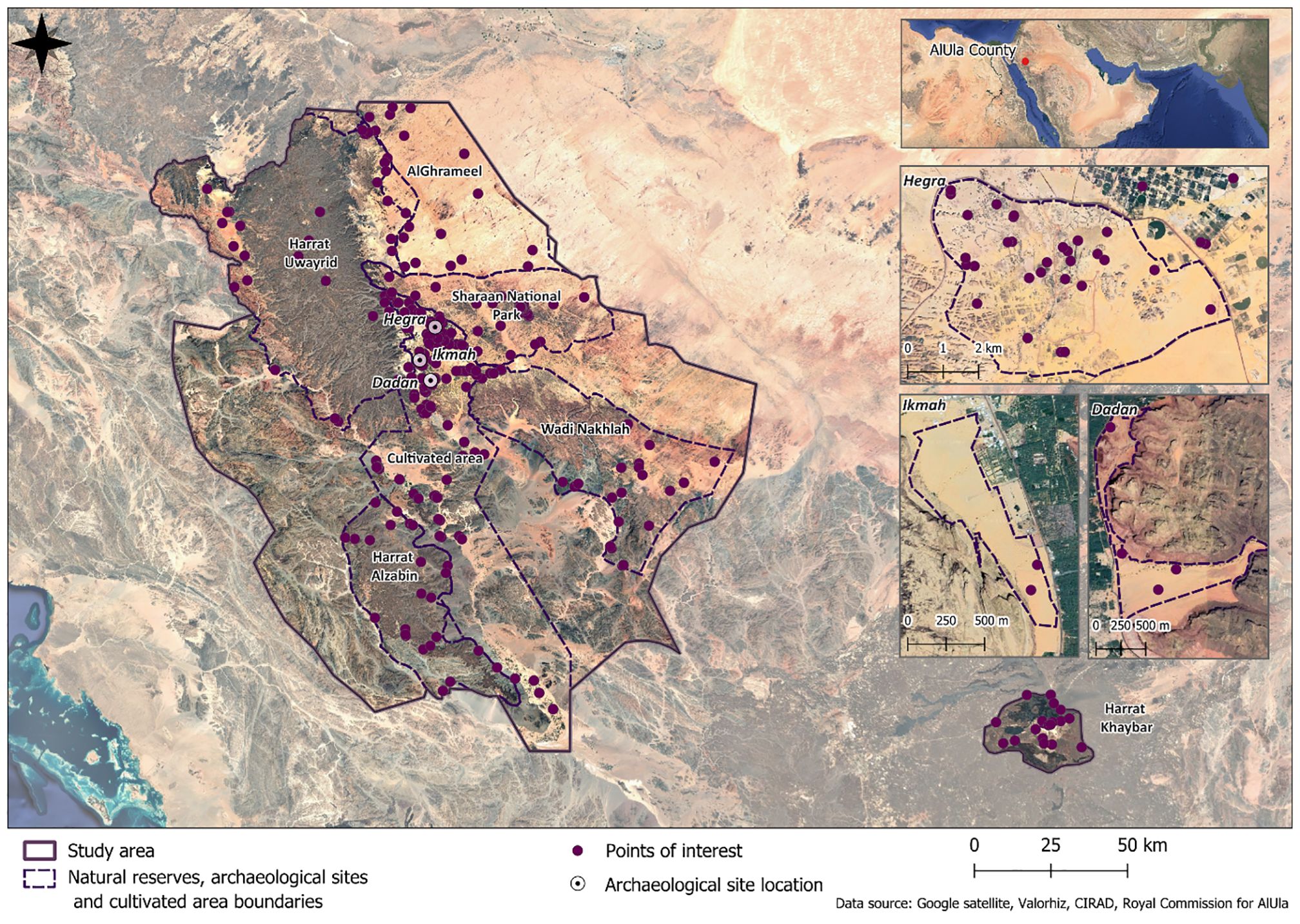
Figure 1. Spatial distribution of soil sampling locations in AlUla region, Saudi Arabia.

A total of 579 soil samples were collected between 2019 and 2024 as part of different projects founded by the French Agency for AlUla Development (AFALULA) and the Royal Commission for AlUla (RCU) which aimed to characterize the diversity of soils and flora in the region of AlUla, and to manage ecological restoration of degraded sites. For each soil sample, a pit of 50cm in length x 50cm in large x 40cm in depth was dug. For each pit, five sub-samples of near 200g were collected between 30 and 40cm depth at the center, north, south, east, and west directions, before being mixed together (for a total of 1kg per soil sample) and sieved at 2mm for further analyses.

2.2 Soil physico-chemical properties

The following physical and chemical variables were measured by COFRAC-certified laboratories (www.aurea.eu, www.laboratoire-teyssier.com and www.celesta-lab.fr) using normative techniques (French or International standards, Supplementary Table S1): clay (%), silt (%), sand (%), pH (water), pH (KCl), resistivity (ohm.cm), electrical conductivity (EC; mS/m), total CaCO₃ (%), P₂O₅ (Olsen method; mg/kg), exchangeable K₂O (mg/kg), exchangeable MgO (mg/kg), exchangeable Na₂O (mg/kg), exchangeable CaO (mg/kg), CEC (cmol/kg), DTPA Fe (mg/kg), DTPA Mn (mg/kg), and Boron (mg/kg). Soil organic carbon (SOC; %) and soil inorganic carbon (SIC; %) were measured using the Rock-Eval analysis (32). Since different projects had different needs, not all these variables were measured on all the samples. For example, 202 samples were analyzed only with Rock-eval. Since texture data is also a compositional data, a CLR transformation was performed before modelling. For other physical and chemical variables, depending on the distribution, data transformation was performed to reduce skewness. The transformations were typically decimal logarithms, except for the pH measurements (no transformation), resistivity (square root transformation), and EC (square root of decimal logarithm).

2.3 X-Ray Fluorescence spectra acquisition and transformation

X-Ray Fluorescence (XRF) data were acquired using the portable XRF S1 Titan analyzer 800 (Bruker, Billerica, Massachusetts, USA), which provided the predicted relative abundance of atomic elements (called here raw data, compared to CLR transformed data) by the equipment software, from magnesium to uranium, based on measured spectral intensities. For each soil sample, XRF acquisitions were conducted on three independent soil sub-samples (loose powder) with three replicates per sub-sample, resulting in a total of nine acquisitions per sample using the “geo-exploration” mode of the XRF S1 Titan analyzer (measurement consisted of three phases). For this equipment, based on constructor information, the voltage ranges from 5 to 50 kV, with a maximum current of 200 μA, and a multi-filter with 5 positions selected automatically by the apparel. The atmospheric measurement environment is air. Absence of detection was replaced by 10 ^-6 values (0.01 ppm) to deal with the problem of zero values in compositional data (16), with the assumption of elements being trace elements at least. When the presence of elements was detected below the limit of detection (< LOD), the limit value for each element, as indicated by the constructor, was used as replacements (Supplementary Table S2). The geometric mean was then calculated for the nine measurements. These replacements allow us to perform CLR transformation (17) without losing the distinction between measured values, detected elements but not measured (LOD) and non-detected elements (represented as one ppm). The CLR transformation is used to open the matrix and to show the relative contribution of each element to the whole composition. It is obtained with the following formula:

$$clr(x_i)=\log (\frac{x_i}{g(x)})$$

With: ${\displaystyle {\sum }_{i=1}^{n}clr}(x_i)=0$, and the geometric mean $g(x)= e^{\frac{1}{n}{\displaystyle {\sum }_{i=1}^n\log }(x_i)}$.

The CLR transformation is made after a first selection of elements based on the sample size and raw element variability. If the threshold for variability is set at 10, we would expect n/10 unique values for one element, eliminating the ones where we have too many LOD values or 10–⁶ replacements (limit or absence of detection). Elements with an absence of variation (i.e., those with a standard deviation of 0) are discarded during this process. After performing the CLR transformation, a second element selection is conducted with a stricter or equal threshold, still applied on the raw values. This step ensures that only the most significant elements, in terms of their contribution to describing the dataset, are retained. However, by keeping some elements before the CLR transformation, we kept the information of less significant elements which are part of the composition. The two thresholds were optimized by testing different values for the first and second selection of variables, allowing us to determine which elements should be retained or discarded from the compositional data. Therefore, each physical and chemical predicted variables had their own set of elements selected. Principal Component Analysis (PCA) was performed over the whole XRF dataset after elements selection and CLR transformation, with a threshold of 10 for the first selection, and 2 for the second, to describe overall sample variability.

2.4 Models’ construction and evaluation

For each predicted variable, samples were separated in a calibration and a validation dataset, based on the Kennard–Stone algorithm (33), with the aim of covering the entire distribution of the dataset, including extreme points. The calibration dataset represented 80% of each chemical variable dataset (112 samples minimum and 282 samples maximum depending of available data, Table 1). LWPLSR (29) was then performed on the calibration dataset. The LWPLSR model maximizes the covariance with the response variable (soil properties) through latent variables (LV) which are orthogonal and built as linear regression of explanatory variables (XRF CLR values). Since it is locally weighted, one model is produced for each XRF data, and is based only on a few samples, selected from the calibration dataset. This selection is based on the Mahalanobis distance between the XRF data of a new sample and the XRF data of all the samples from the calibration dataset. Number of samples selected using this distance was set to 30. This number could be lower if outliers (high distance) were detected and are then assigned with a weight of 0. For the other selected samples, weight is calculated as an exponential function based on Mahalanobis distances between samples:

Table 1

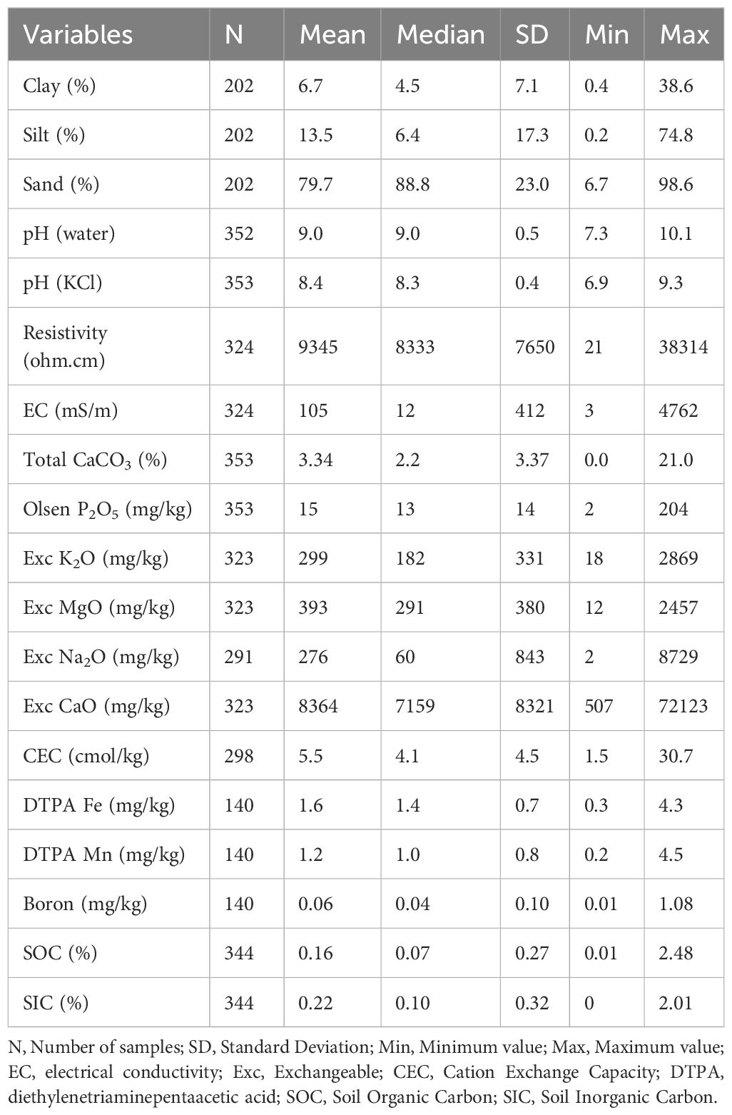
Table 1. Soil physical and chemical variables measured and their respective statistics.

$$w_{i,j}= e^{\frac{- d_{i,j}}{h.MAD(d_j)}}$$

Where $w_{i,j}$ is the weight and $d_{i,j}$ is the Mahalanobis distance of the calibration sample i with the validation sample j. MAD is the median absolute deviation of the Mahalanobis distances for the validation sample j. The coefficient h is the sharpness of the weight function and was set to 1. The weights are then normalized between 0 and 1.

Optimal number of LVs (1 to 10 were tested) was obtained through 6-fold cross-validation (randomly selected over the calibration dataset) repeated 3 times, using a precision gain ratio R_g. Gain in root mean square error of cross-validation (RMSECV) is calculated for each LV and the optimal number is set when R_g does not further improve (threshold of 0.02). Then, for each sample of the validation set, each variable was predicted using the calibration set. Model performance was evaluated using:

- The Root Mean Squared Error of Prediction (RMSEP) over the validation set.

- The coefficient of determination R² between prediction and measured values in the validation set (inverse CLR is performed for the texture).

- The Ratio of Performance to Deviation (RPD), being the standard deviation (SD) divided by RMSEP (the performance), which should be over 2 for good model performance (34) and which indicates an untrusted model with values below 1.4.

- The Ratio of Performance to Inter-Quartile (RPIQ). Inter-Quartile Range (IQR) being the difference between third and first quartile replacing SD in the RPD, which is more appropriate if a variable is not normally distributed (35). Successful predictions were defined with RPIQ > 1.9 (36), acceptable predictive power was associated with RPIQ between 1.7 and 1.9 (37).

Mean VIP were calculated over the calibration dataset for each element to determine which were most important (31). This method allows the identification of atomic elements for which the relative contribution to the XRF data has the highest impact on studied variables.

Effects of CLR transformation for composition data (XRF and texture), as well as chosen model between LWPLSR and PLSR, were tested for the different variables under study. RMSEP and R² were computed to evaluate each method combination. Modelling and analysis were performed using the R software language (38), with FactoMineR package (39) for PCA, and with the rnirs and rchemo packages (29, 40) for LWPLSR and PLSR.

3 Results

3.1 Soil physical and chemical properties

Measured sand, silt and clay content covered different texture class based on the USDA triangle texture classification (Figure 2). The majority of samples (87%) were classified as: Sand, Sandy Loam and Loamy Sand soils, and a minority (13%) as: Sandy Clay Loam, Loam, Silty Loam and Silty Clay Loam. Sand content distribution was the most extended over the soil samples with values between 7% and 99% (Table 1), and half of the samples had a sand content above 89%. The silt content was distributed on a gradient from 0.2% to 75%, with an uneven distribution (median = 6%). The clay content range was the lowest with a maximum of 39%, and half of samples below 4.5% (narrowing the full texture gradient studied). Additionally, three classes of texture were not covered: Clay, Sandy Clay and Silt (Figure 2).

Figure 2

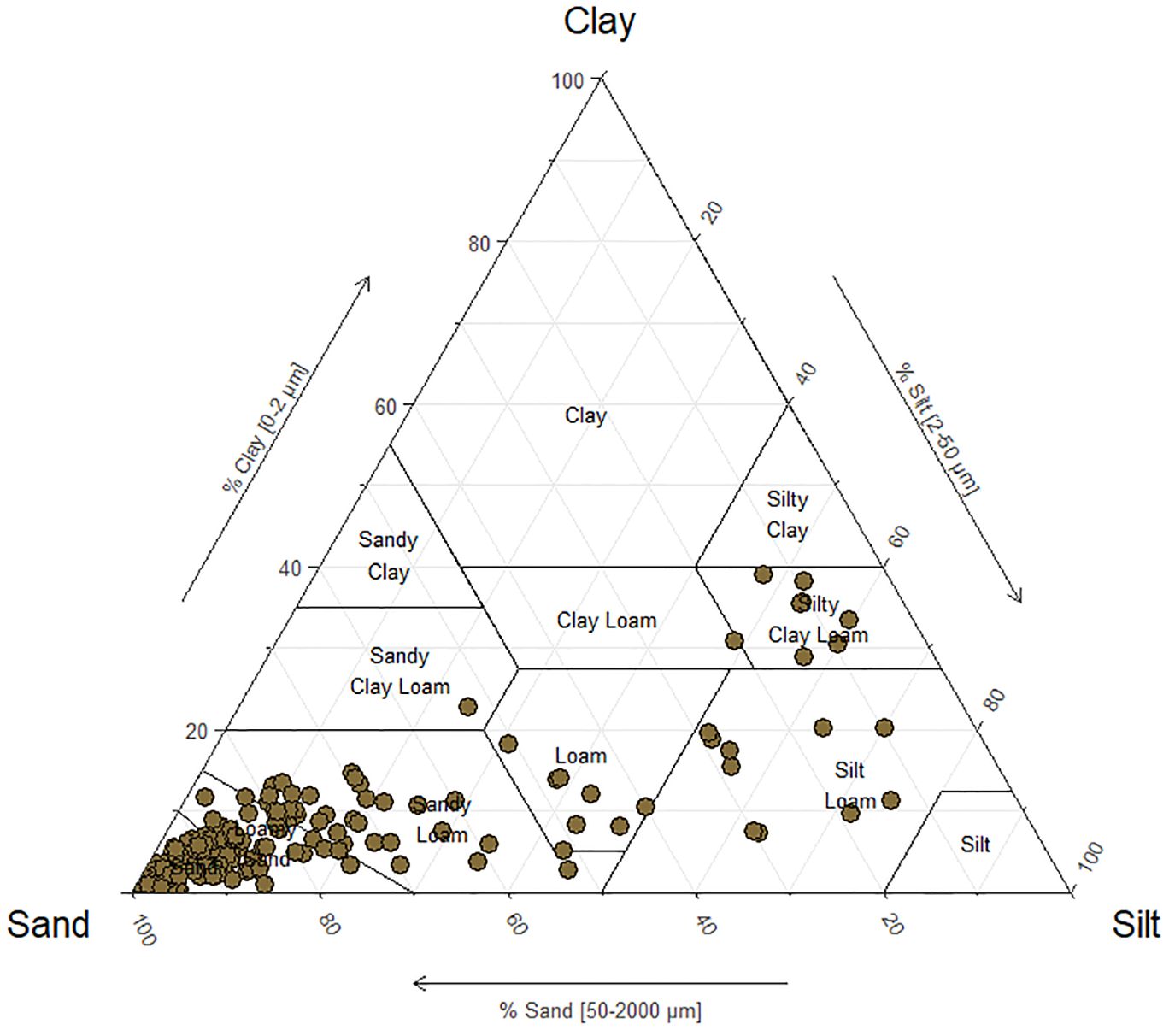
Figure 2. Clay, silt and sand content for 202 samples placed on the USDA texture triangle (52).

Other measured chemical properties are described in Table 1. Soil pH measured in water varied from 7.3 to 10.1, classifying the samples from neutral to strongly alkaline. Soil resistivity (and EC) showed a wide variability, from 21 to 38,314 ohm.cm, and a very uneven distribution, with a skewness of 8.9 for EC. About 10% of the samples had a resistivity below 500 ohm.cm, classifying them as corrosive. Most of the samples had a total CaCO₃ content below 20%, classifying as non-calcareous. Other macro and micro-elements measured had an uneven distribution, with skewness values ranging from 1.4 (DTPA Fe) to 8.6 (Olsen P₂O₅). Exchangeable CaO was the highest of the macro-elements (8364 mg/kg on average), while Na₂O was the lowest (276 mg/kg on average). Low content and uneven distributions were also found for organic and inorganic carbon, with a mean of 0.16% and 0.22% respectively.

Distribution of calibration and validation dataset for each studied variable, selected with the Kennard-Stone algorithm, is represented in Figure 3. The figure demonstrates a relatively similar distribution between both datasets.

Figure 3

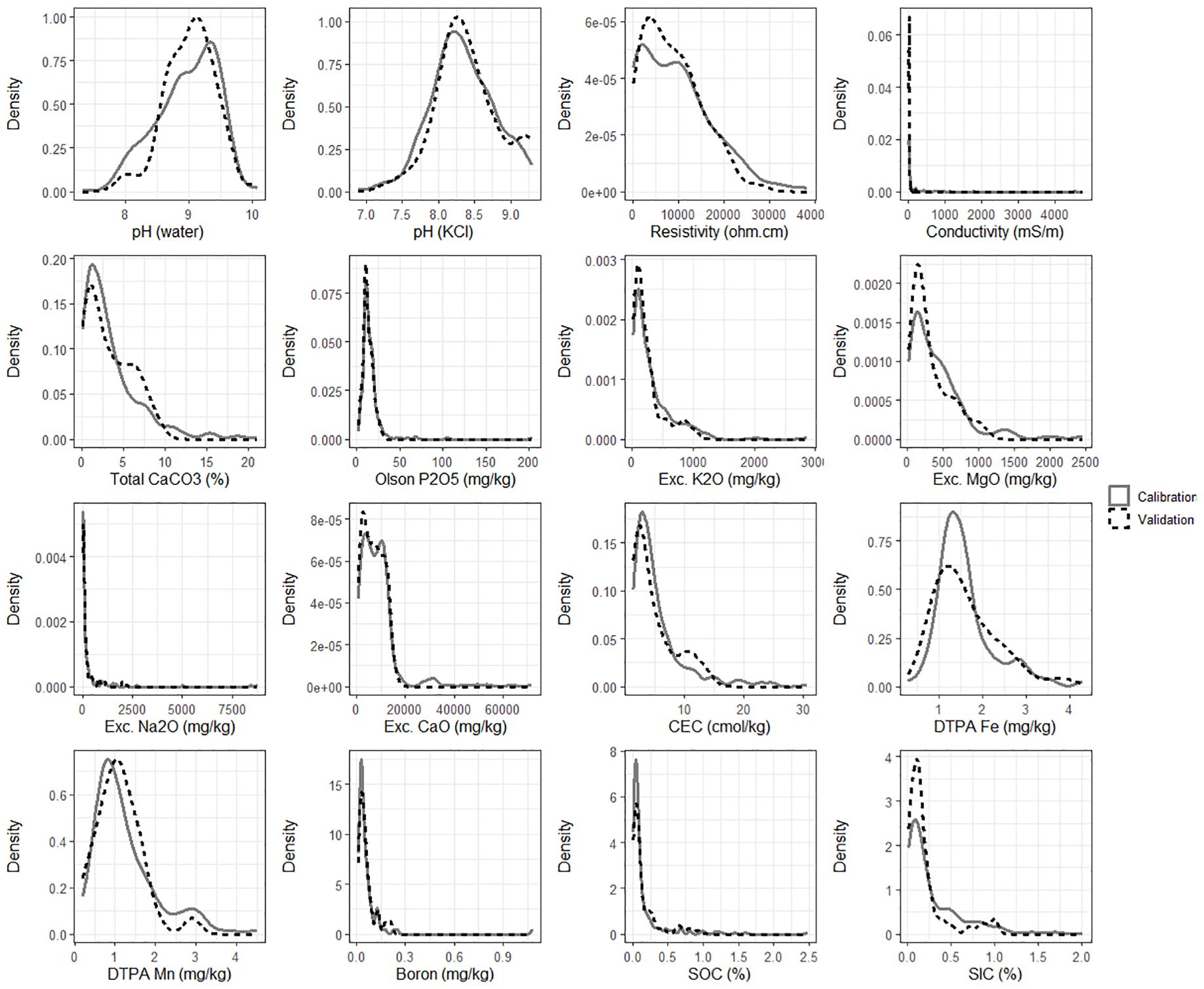
Figure 3. Density plots for each soil property showing the calibration and validation datasets.

3.2 Description of XRF data

To describe XRF data, we first selected 29 atomic elements based on a threshold of at least 58 different values across the 579 samples (1/10 of the samples). CLR transformation was then performed on those elements. Following this, 18 atomic elements were selected for the PCA based on a second threshold of at least 290 different values (also in the raw data) through the 579 samples (half of the samples). Considering the first four principal components, 74% of soil samples variability was explained including 57% by the first two axes (Figure 4).

Figure 4

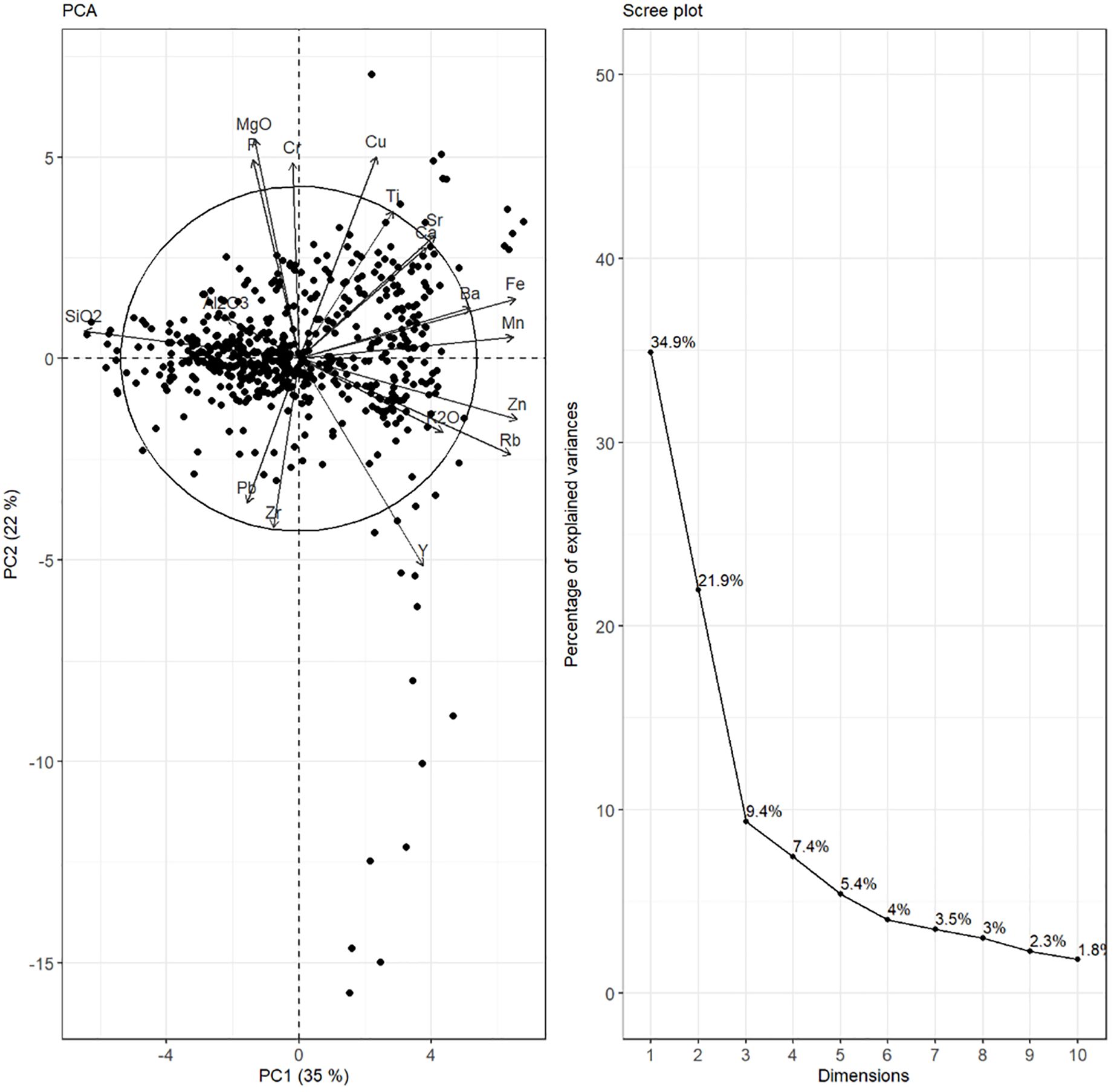
Figure 4. Biplots and scree plot of the principal component analysis (PCA) performed over 579 samples and 18 selected CLR-transformed XRF variables.

Since XRF data was CLR-transformed, the PCA shows the relationship between elements that have a similar relative contribution to each sample composition (high or low measured values compared to the geometric mean). The global distribution along the first two axes revealed three important directions. The first one shows an enrichment in SiO₂ and impoverishment in K₂O, Mn, Fe and Zn (corresponding to sandy and clayey soils). The second one was represented by the elements Cu and Ca being more present, and Pb being more absent (silty and clayey soils). The third one was driven by Zr on the positive side and MgO, P and Cr on the negative side (silty and sandy soils). The gradients of each texture variable represented on the PCA, showing these three directions, can be found in Supplementary Figure S1.

3.3 LWPLSR model performances

3.3.1 Prediction of soil texture

For texture variables (clay, silt and sand), the best model performance was found by predicting the CLR values of clay content and silt content. Sand content was calculated from the two other variables since the sum of CLR values is equal to zero. Using the precision gain ratio (R_g), the optimal number of latent variables (LVs) was one. RMSEPs for the validation dataset were below 6% for the three texture variables (Figure 5A), with RPD > 2 for the three variables and RPIQ > 1.9 for sand and clay. Only silt content had a RPIQ lower than this threshold but above 1.7. Nonetheless, the R² values for each texture variable were high (R² > 0.85), meaning accurate predictions. Clay content prediction had the best performance (R² = 0.96 and RPIQ = 2.6), followed by sand content prediction (R² = 0.93 and RPIQ = 2.36).

Figure 5

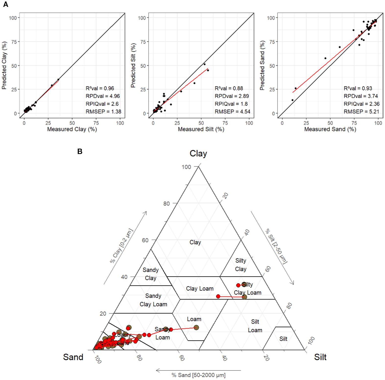
Figure 5. Predicted vs. measured texture variables for the validation set shown for each size category content (A) and on the USDA texture triangle (predicted values in red) (B).

Validation set representation over the USDA texture triangle was completed with the predicted values (Figure 5B). The texture classes of Loam and Silty Clay Loam had a small amount of sample representativity, with only two points with clay content over 20%. Change of texture class was observed only for 7 samples, but occurred only between adjacent classes between predicted and measured values.

3.3.2 Prediction of soil chemical variables

For other soil properties, we found different model performances, as described in Table 2. Based on VIP values, the three main predictors were identified for each predicted variable. Relationship between predicted and measured values is represented in Figure 6. Poor prediction performances (RPIQ < 1.4) were found for the extractable micro-elements Mn and Boron, Olsen P₂O₅, exchangeable Na₂O and EC. Interestingly, P content measured by XRF was not found in the main predictors based on VIP for P₂O₅. On the contrary, Mn content was placed third for DTPA Mn.

Table 2

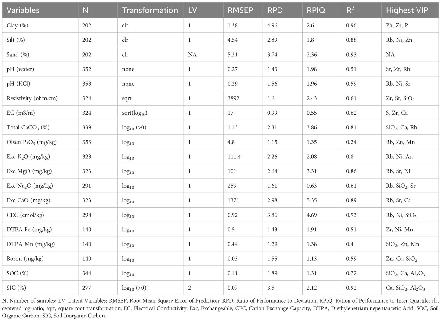
Table 2. Modelling performance (validation datasets) for each soil physical and chemical variable.

Figure 6

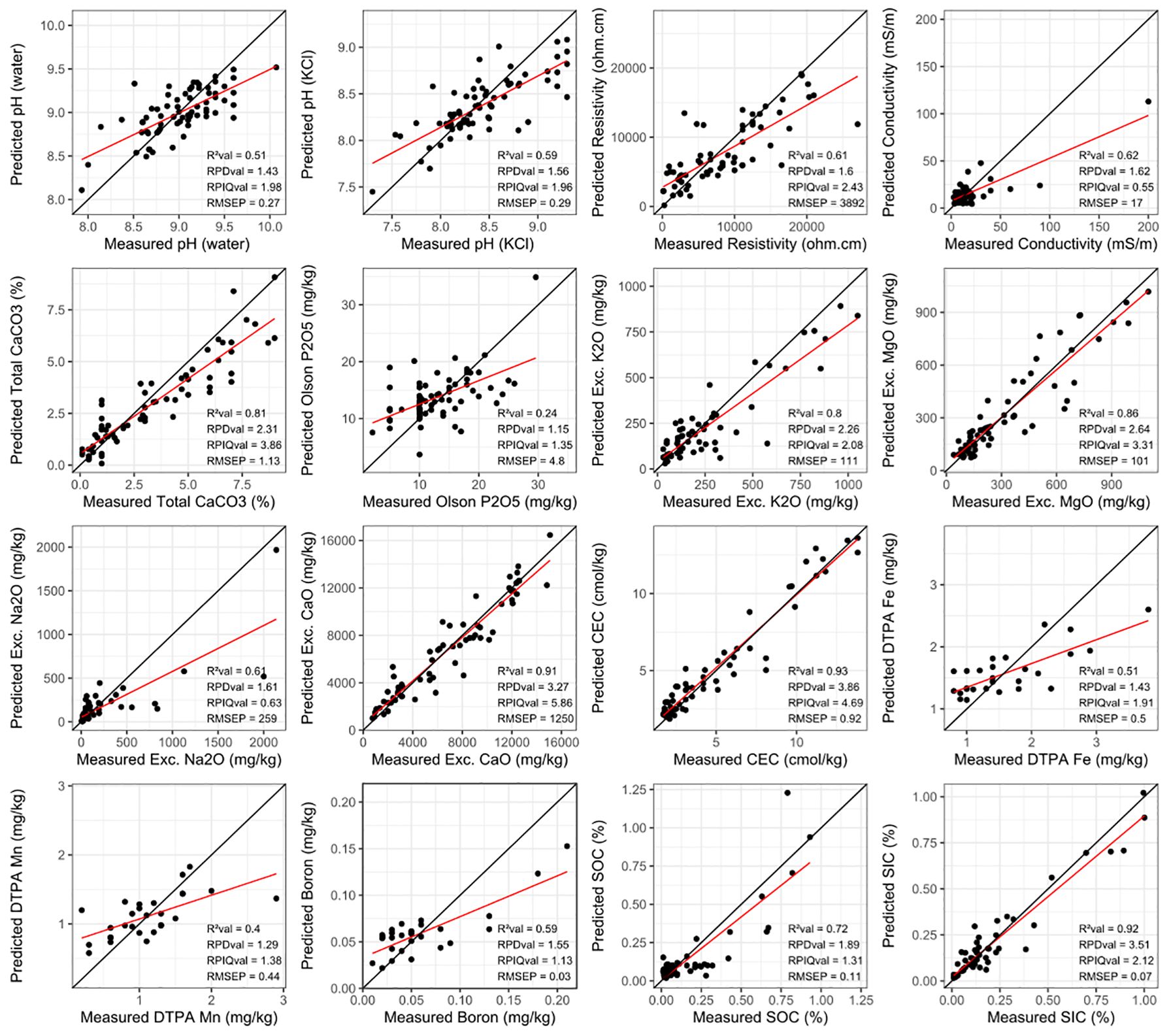
Figure 6. Predicted chemical variables from the validation datasets vs. measured variables.

Acceptable model performances (RPD > 1.4; RPIQ > 1.9) were found for resistivity, the two types of pH, and DTPA Fe (Table 2). SOC had medium performance with a high R² (0.72) and low RPIQ (1.31). For extractable Fe, Fe content measured by XRF did not feature in the three main predictors; but rather Zr, Ni and Mn. pH (KCl) had a higher RPD and R² values compared to pH (water) and shared Rb and Sr as their variables with highest VIP.

Excellent LWPLSR model performances (RPD > 2.2; RPIQ > 2) were found for six chemical variables: CEC, exchangeable MgO, CaO and K₂O, total CaCO₃, and SIC (Table 2). R² values were above 0.8. Rb content was placed first predictor for all exchangeable macro-elements. For SIC, Total CaCO₃, and exchangeable CaO, Ca content provided by the XRF data appeared as one of the three highest variables in terms of VIP, as expected. The best prediction performances were found for the CEC variable (R² = 0.93; RPD = 3.86 and RPIQ = 4.69), with Rb, Ni and SiO₂ measured by XRF as the main predictors.

3.4 Methodology comparison

To assess the contribution of CLR transformation on compositional data and LWPLSR, we tested separately the effect of using raw compositional data (for XRF and texture data) compared to the transformed ones, as well as the classic global PLS regressions method compared to the locally weighted one.

Modelling performances of each methodology combination regarding texture variables are presented in Table 3. With PLSR model, the change between raw values to CLR-transformed values showed better performance, as reflected by higher R² values. The performance increase was more important for clay when XRF data was CLR-transformed (R² of 0.41 for clay, 0.07 for silt, and 0.21 for sand). In comparison, for texture data, CLR transformation resulted in better predictions for sand and silt, with R² of 0.19 for clay, 0.38 for silt and 0.33 for sand. Nonetheless, it is the combination of both that gave the best indicators with global PLSR model (lowest RMSEP for silt and sand).

Table 3

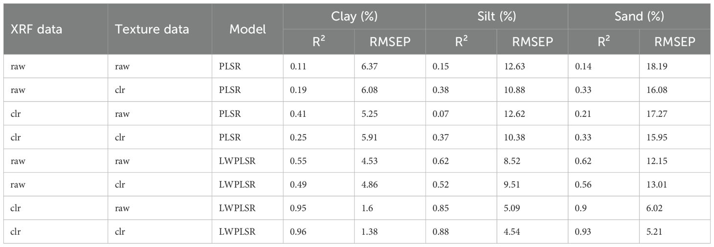
Table 3. Modelling performance (validation sets) for texture based on transformation and PLSR type.

Using LWPLSR model, indicators were found higher compared to global PLSR when using raw data, with R² = 0.62 for silt and sand content, and R² = 0.55 for clay content. The performances of each prediction were the highest when both XRF data and texture was CLR-transformed. The greatest improvement was found when XRF data was CLR-transformed, with RMSEP being two times lower than that obtained with raw data.

For the other chemical variables, modelling performances can be found in Table 4. For all variables, the lowest RMSEP was found using LWPLSR with CLR-transformed XRF data. For global PLSR, CLR-transformed XRF data improved R² except for Total CaCO₃. Similarly, for LWPLSR, CLR transformation enhanced the R² values, except for EC. Transitioning from PLSR model to LWPLSR model resulted in the highest R² values and the lowest RMSEP for all variables.

Table 4

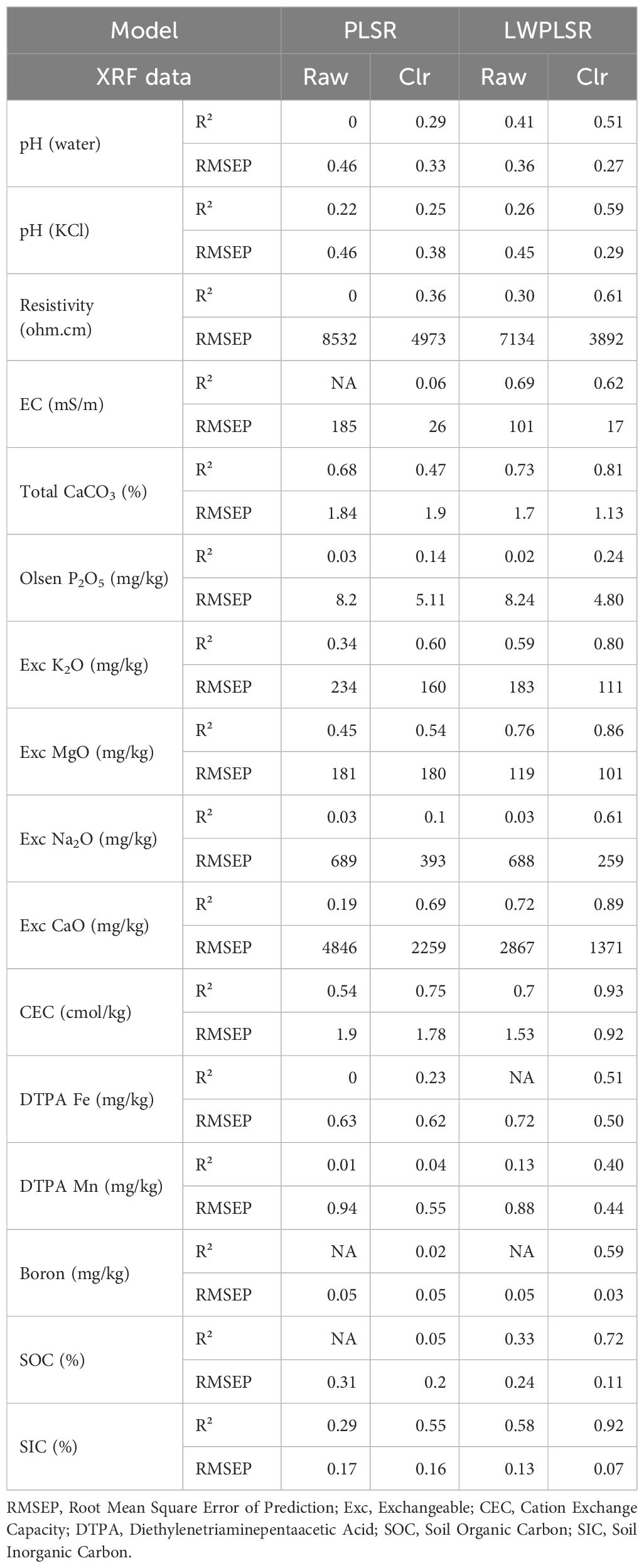
Table 4. Modelling performance (validation sets) for chemical variables based on PLSR type and XRF data used.

4 Discussion

4.1 Predictions of soil variables with XRF data

Few soil texture classes were represented in the sampling study with a huge majority in the sand, sandy loam, and loamy sand texture class (Figure 2). This specificity was linked to a desertic environment and representative of hyperarid soils found in Saudi Arabia (41).

Using XRF spectrometry, combined with CLR transformation and locally weighted PLSR, we found good prediction performances for soil texture (R² > 0.88, RPIQ > 2.3 for sand and clay). Previous studies have reported similar prediction potential for soil texture using XRF data in various environments, including tropical (9), subtropical (12, 22), and continental (23) climates. Nonetheless, in a hyperarid environment, combining raw XRF data and PLSR models has proven inefficient in predicting soil texture using PLSR (28), which aligns with the results of this study (Table 3).

Different methodologies have been explored in previous studies for soil texture, such as multiple linear regression (MLR) (12, 22) and random forest (9), those could be effective methods since particles size distribution was greater and covering many texture classes compared to hyperarid environments. In contrast, indicators values in our study were higher for sand, silt, and clay content predictions using LWPLSR (Figure 5). However, since hyperarid environments are predominantly composed of sandy texture classes, the number of samples in our study is very low for other classes. While clay content prediction performed excellently, applying the model to silty-clayey soils in hyperarid environments may require further investigation.

Combined methodologies including XRF spectra have also been previously explored to predict soil texture: using the XRF spectra obtained from the two beams (different energy range) after processing and PCA rather than the elemental content calculated from it, or using XRF data coupled with near-infrared (NIR) spectra (22, 23). In these works, PLSR, MLR and cubist models (decisional tree) were used, showing good performances in subtropical and continental contexts. Cubist model gave the best performance (RPIQ > 3) in a continental context, but R² was found below 0.5 regarding Sand and Loamy Sand classes for silt and sand content predictions (23). Nevertheless, these studies did not explore CLR transformation XRF data, not taking into account the properties of compositional data (17). Moreover, decisional trees lack interpretative results compared to PLS regressions or MLR, such as the individual contribution of each explanatory variable, using for example VIP.

Measured soil chemical variable values were representative of hyperarid environments (42), with low soil organic carbon and low plant nutrient availability (low P, N, Fe or Zn) (Table 1). We also found mostly alkaline pH, with some calcareous soils, and some areas with high salinization (high EC) which can lead to low fertility or the development of specific plant communities with high tolerance to these harsh conditions (43).

Given the specific conditions of this environment, depending on soil chemical variables studied, predictions showed a high level of variation (Table 2) in terms of performances using XRF data and LWPLSR. Low model performance was found for Mehlich-3 P by XRF (44), similar to exchangeable P using resin extraction in tropical contexts (45), which is in accordance with the R² of 0.24 found for Olsen P₂O₅ (sodium bicarbonate) measured in our study. Phosphorus has indeed a complex cycle in soil with unavailable forms, associated with Fe and Al oxides, in organic matter or in other mineral forms, bound with Ca or Mg (46). This makes it difficult to link P content found with XRF with the plant available form, explaining the absence of P in the main predictors for Olsen P₂O₅.

Similarly, electrical conductivity (EC), as well as water pH are mostly linked to atomic element forms (ionic or more stable), which is not given by XRF measurements. Therefore, this could influence prediction performances for these variables (poor and medium performances). Yet, in arid context, using XRF data and PLSR, EC showed good predictions (R² = 0.84), but contrary to our data (skewness of 8.9) they were made in a more homogeneous salinity level, less sandy soils and more calcareous (28).

For water pH, prediction performances showed a high variability in literature (R² varied from 0.12 to 0.77) using MLR, PLSR, decisional tree and CNN (convolutional neural network) from temperate to tropical context (13, 23, 27, 45). In (27), which presented the best predictions performances, pH values ranged from 4.2 to 8.6 in a continental context. This was very different compared to the pH range found in our sampling study going from 7.3 to 10.1 in a desertic region, where our model still provided acceptable performance (RPD > 1.4; RPIQ > 1.9). Since extraction methodology differed for macro-elements (resin extraction, nitric acid or ammonium lactate) model performances comparison is more complicated (13, 14, 45).

In tropical context or when using CNN method, good predictions for K and Na content have been reported, which was also the case for exchangeable K₂O in hyperarid context, but not for Na₂O. Given the range of elements analyzed with XRF, organic elements (C and N) are not identified. Nevertheless, medium performances were identified for soil organic carbon. This may be explained by the known interactions with clay or Fe/Al oxides (15, 47) whose elements are measured by XRF.

Good prediction performances were observed for total CaCO₃ content, SIC, exchangeable Ca, Mg and K₂O, as well as CEC (Figure 6). In an arid context, with more calcareous soils (6 to 75%), good predictions of total CaCO₃ were also reported using PLSR (28). Extractable Ca and Mg (with ammonium lactate) predictions with XRF, showed high R² values (0.9) in temperate climates (26), which is in accordance with our results for exchangeable CaO and MgO predictions, despite the usage of a different solvent (ammonium acetate). Finally, the variable CEC usually was predicted with high accuracy: in a continental context using MLR with R² of 0.91 (24) or reaching 0.82 of R² using SVM modelling and VNIRS fusion added to XRF data in a subtropical climate (25). In our study, using LWPLSR with CLR-transformed XRF data, we achieved the highest performance, with an R² of 0.93.

4.2 Atomic elements involved in prediction models

Since LWPLSR allows for the calculation of VIP, we were able to identify the main elements used in each model (Table 2). This allows better comprehension of each model and its potential coherence.

Relationship between Rubidium measurements via XRF and soil texture has been well-established in previous studies (12, 22, 23, 48), and our findings confirm this by identifying Rb as one of the main predictors. Similarly, elements such as Zn and Zr, which were important in our study, have also often been associated with clay and sand prediction in these previous studies. Regarding Pb being the main predictor for clay content, relationship between clay and Pb has been reported through the existence of adsorption mechanisms (49). Since CEC is related to exchangeable cations, similar predictors were founded like Rb, Ni and Sr. In comparison, none of these three elements were found in the MLR developed in (24) for CEC, but this study was conducted on soils belonging to classes with higher silt and clay content. For Total CaCO₃, SIC as well as exchangeable CaO had Ca as its main predictors, which was a coherent result. However, for Exchangeable MgO and K₂O, we did not find their respective element measured by XRF as their main predictors. Indeed, availability of cations is based on other molecular interactions and soil pH (15). Therefore, while XRF can capture the overall composition, it does not directly provide specific information regarding the availability of these cations. Fe measured by XRF and DTPA has been shown having different distributions in soils because of the different forms and solubility of iron (50) which could explained the absence of Fe in the variables having the highest VIP for DTPA Fe.

By definition, XRF does not measure element content for atomic number below 12 (Mg), which includes Sodium (Na), Carbon (C), and Boron (B), all showed medium to poor prediction performances. Yet, they were tested in this study since their association with heavier elements have been acknowledged, therefore the variables could have been deducted using the others elements. Indeed, an exception was when carbon, in combination with calcium (Ca), was used to predict SIC and total CaCO₃. And, Al₂O₃ was found to be a main predictor for SOC, which can be explained by known interactions between organic matter and Al oxides (47).

4.3 Advantages of CLR on compositional data and LWPLSR

The methodology used for modelling was the locally weighted PLS regression combined with the CLR transformation of compositional data. Log-ratio transformation was proposed by Aitchison (16) to avoid difficulties encountered when dealing with compositional data being a closed matrix where correlations between ratio are misleading. Log-ratio can be additive, isometric or centered. This is the third one that was selected as a suitable transformation to describe compositional data produced by XRF methodology, compared to their raw values or log-transformed (17). This data showed better properties in Euclidean spaces such as in PCA. Despite sometimes being used to calibrate XRF data (19, 20), it was not found in the literature as a tool to preprocess XRF data before predictions. We found in Table 3 and Table 4 a strong improvement in model performances when CLR transformation was applied for XRF data or texture, in a hyperarid environment. This method should therefore be tested in more environments or modelling types to study the potential in increased prediction accuracy.

In a similar way, we showed the prediction improvement by using LWPLSR rather than PLSR (Table 3, Table 4). LWPLSR was initially developed to enhance the prediction of soil organic carbon using VNIR spectra (29) and was later applied to other soil properties, and proved to be more effective than global PLSR (30, 51). In fact, by producing specific models for each prediction on a smaller number of samples combined with statistical weights, LWPLSR can better deal with non-linearity of complex data, but at the same time, it makes LWPLSR highly dependent on a very representative calibration dataset. Compared to more advanced machine learning methods like SVM, Random Forest and CNN, LWPLSR is able to show importance of elements (or wavelengths for VNIRS) using the b-coefficients of the model or the VIP values (31), allowing good interpretability. Moreover, LWPLSR showed similar or better model performances (Table 2) for texture predictions compared to SVM, Gaussian, Random Forest (9) or the Cubist model (23). Thus, in an arid context, where soil texture predictions using raw XRF data and global PLSR gave unreliable results (28), we found good model predictions by combining these two methodologies.

4.4 Limitations and prospects

This study showed the possibility to predict some physical and chemical soil variables with good model performance. However, some variables proved more challenging to predict, based on the complexity of their cycle and different forms as well as the absence of their element being measured directly by the XRF (C, B, Na). To expand the number of soil variables that can be predicted, exploring other modelling methodologies, such as machine learning and deep learning, may be beneficial. Previous studies have shown good predictions using Random Forest for extractable Cu and Mn (44), K content (14), with SVM for CEC (25) or with CNN for pH (13).

The performance of LWPLSR is very dependent on the representativity of the dataset, since it is based on the similarity between the input variables (XRF or VNIR spectra). To improve model accuracy, it is essential to have a large and diverse dataset, which can be time- and cost- consuming. Given that, hyperarid environments are mostly dominated by sandy soils, other soil types were underrepresented in this study. Further investigations are needed to ensure broader applicability across different soil types. Additionally, since each prediction is based on a new model limited to a subsample of the calibration dataset, it has to be as clean and representative as possible. Therefore, large datasets allow the identification of the best spectral neighbors for each prediction, as shown by Cambou (51).

Combining XRF spectra with other spectroscopic technologies, such as visible and near-infrared (VNIR), mid-infrared (MIR) or short-wave infrared (SWIR), has been widely discussed in the literature (13, 22, 25, 26, 45). These technologies are already known to give information about soil content through absorption at given wavelength corresponding to characteristic vibrational bands. Organic matter properties, soil mineralogy and texture, pH, and concentrations of macro and micro-elements, have all been successfully predicted using VNIRS technology (11). Similar to the XRF analysis, VNIRS is time- and cost-effective but also non-destructive. They could therefore be combined together to improve soil variables prediction, in particular since VNIRS can detect organic compounds linked to carbon (C) and nitrogen (N), atoms that cannot be detected by XRF. Indeed, soil organic carbon and nitrogen have shown good prediction performances using VNIRS data (30, 51). Fusion methods have also been developed, such as using principal components of NIR spectra (22), least squares (LS), Granger-Ramanathan (GR), and Outer Product Analysis (OPA) for combining XRF and VNIRS (26).

By decreasing the time needed to analyze a great number of samples, the models developed in this study can be applied to predict soil physical and chemical properties of other soil samples collected in the AlUla region. These models can support various scientific topics (e.g. in environmental or agricultural studies) and need to be challenged on soils collected from other hyperarid environments. Since aridification of many environments are expected by climatic models, fast and large-scale characterization of soils will be an important tool to better understand soil functioning and to design relevant soil management strategies for various purposes (agriculture, ecological restoration strategies). These time- and cost-efficient methods will also allow designing high-resolution monitoring regarding soil fertility, salinization, and erosion at large-scale (42) and link these parameters to crop productivity and changes in natural plant communities.

5 Conclusion

XRF data acquisitions were carried out on soil samples to predict soil texture and several chemical properties in the hyperarid environment of the AlUla region, in Saudi Arabia. Soil samples were dominated by a sandy texture with low clay content. An innovative approach was used by combining CLR transformation on compositional data and locally weighted partial least squares regression (LWPLSR) modelling. Reliable models were developed for soil texture, particularly for the clay and sand soil fractions in hyperarid soils. The respective effects of data transformation and locally weighted regression were tested showing the importance of CLR transformation for XRF data and the relevance of LWPLSR. High model performances were also found for total CaCO₃, exchangeable Ca, Mg and K, as well as CEC. Acceptable model performances were observed for pH (water and KCl), resistivity, DTPA Fe, and SOC. On the contrary, EC, available P, Na, Mn, and B did not show acceptable model performances. The limitations in modelling could be linked to the environment conditions and the inherent constraints of XRF technology, which does not provide information on elements with atomic numbers lower than Mg or the atomic form (ionic or bonded). Overall, using prediction models from spectrometry data represents a significant technological advancement for large-scale soil property characterization and monitoring at low cost.

Data availability statement

The raw data supporting the conclusions of this article will be made available by the authors, without undue reservation.

Author contributions

BK: Data curation, Writing – review & editing, Methodology, Conceptualization, Writing – original draft, Visualization, Formal Analysis, Validation. SB: Supervision, Writing – review & editing. OM: Writing – review & editing, Supervision. YF: Writing – review & editing, Supervision. HB: Resources, Writing – review & editing, Supervision, Project administration, Funding acquisition. SA: Writing – review & editing, Supervision. SR: Supervision, Writing – review & editing. BL: Supervision, Writing – review & editing. AM: Writing – review & editing, Supervision. AA: Writing – review & editing, Supervision.

Funding

The author(s) declare financial support was received for the research and/or publication of this article. This research was funded by the Royal Commission for AlUla, AlUla, Saudi Arabia.

Acknowledgments

We would like to thank all those involved in the Sharaan National Park project, and the RCU (Royal Commission for AlUla, Saudi Arabia) and AFALULA (French Agency for the development of AlUla, France) for their financial support. We gratefully thank Julie Berder and Quentin Bachelet (Valorhiz laboratory team) for the XRF acquisitions, Ines Candela (Valorhiz geomatic team) for the study area map, and all the field teams for the soil collection.

Conflict of interest

The authors declare that the research was conducted in the absence of any commercial or financial relationships that could be construed as a potential conflict of interest.

Generative AI statement

The author(s) declare that no Generative AI was used in the creation of this manuscript.

Any alternative text (alt text) provided alongside figures in this article has been generated by Frontiers with the support of artificial intelligence and reasonable efforts have been made to ensure accuracy, including review by the authors wherever possible. If you identify any issues, please contact us.

Publisher’s note

All claims expressed in this article are solely those of the authors and do not necessarily represent those of their affiliated organizations, or those of the publisher, the editors and the reviewers. Any product that may be evaluated in this article, or claim that may be made by its manufacturer, is not guaranteed or endorsed by the publisher.

Supplementary material

The Supplementary Material for this article can be found online at: https://www.frontiersin.org/articles/10.3389/fsoil.2025.1668732/full#supplementary-material

References

1. Durbecq A, Jaunatre R, Buisson E, Cluchier A, and Bischoff A. Identifying reference communities in ecological restoration: the use of environmental conditions driving vegetation composition. Restor Ecol. (2020) 28:1445–53. doi: 10.1111/rec.13232

Crossref Full Text | Google Scholar

2. Schoenholtz SH, Miegroet HV, and Burger JA. A review of chemical and physical properties as indicators of forest soil quality: challenges and opportunities. For Ecol Manage. (2000) 138:335–56. doi: 10.1016/S0378-1127(00)00423-0

Crossref Full Text | Google Scholar

3. Critchley CNR, Chambers BJ, Fowbert JA, Sanderson RA, Bhogal A, and Rose SC. Association between lowland grassland plant communities and soil properties. Biol Conserv. (2002) 105:199–215. doi: 10.1016/S0006-3207(01)00183-5

Crossref Full Text | Google Scholar

4. Fernández MD, Cagigal E, Vega MM, Urzelai A, Babín M, Pro J, et al. Ecological risk assessment of contaminated soils through direct toxicity assessment. Ecotoxicol Environ Saf. (2005) 62:174–84. doi: 10.1016/j.ecoenv.2004.11.013

PubMed Abstract | Crossref Full Text | Google Scholar

5. Maurice K, Bourceret A, Youssef S, Boivin S, Laurent-Webb L, Damasio C, et al. Anthropic disturbances impact the soil microbial network structure and stability to a greater extent than natural disturbances in an arid ecosystem. Sci Total Environ. (2024) 907:167969. doi: 10.1016/j.scitotenv.2023.167969

PubMed Abstract | Crossref Full Text | Google Scholar

6. Bünemann EK, Bongiorno G, Bai Z, Creamer RE, De Deyn G, De Goede R, et al. Soil quality – A critical review. Soil Biol Biochem. (2018) 120:105–25. doi: 10.1016/j.soilbio.2018.01.030

Crossref Full Text | Google Scholar

7. Maurya S, Abraham JS, Somasundaram S, Toteja R, Gupta R, and Makhija S. Indicators for assessment of soil quality: a mini-review. Environ Monit Assess. (2020) 192:604. doi: 10.1007/s10661-020-08556-z

PubMed Abstract | Crossref Full Text | Google Scholar

8. Aldabaa AAA, Weindorf DC, Chakraborty S, Sharma A, and Li B. Combination of proximal and remote sensing methods for rapid soil salinity quantification. Geoderma. (2015) 239–240:34–46. doi: 10.1016/j.geoderma.2014.09.011

Crossref Full Text | Google Scholar

9. Benedet L, Faria WM, Silva SHG, Mancini M, Demattê JAM, Guilherme LRG, et al. Soil texture prediction using portable X-ray fluorescence spectrometry and visible near-infrared diffuse reflectance spectroscopy. Geoderma. (2020) 376:114553. doi: 10.1016/j.geoderma.2020.114553

Crossref Full Text | Google Scholar

10. Cambou A, Cardinael R, Kouakoua E, Villeneuve M, Durand C, and Barthès BG. Prediction of soil organic carbon stock using visible and near infrared reflectance spectroscopy (VNIRS) in the field. Geoderma. (2016) 261:151–9. doi: 10.1016/j.geoderma.2015.07.007

Crossref Full Text | Google Scholar

11. Stenberg B, Viscarra Rossel RA, Mouazen AM, and Wetterlind J. Visible and near infrared spectroscopy in soil science. In: Advances in Agronomy. Amsterdam, Netherlands: Elsevier (2010). p. 163–215. Available online at: https://linkinghub.elsevier.com/retrieve/pii/S0065211310070057. (Accessed September 11, 2025).

Google Scholar

12. Zhu Y, Weindorf DC, and Zhang W. Characterizing soils using a portable X-ray fluorescence spectrometer: 1. Soil texture. Geoderma. (2011) 167–168:167–77. doi: 10.1016/j.geoderma.2011.08.010

Crossref Full Text | Google Scholar

13. Javadi SH, Munnaf MA, and Mouazen AM. Fusion of Vis-NIR and XRF spectra for estimation of key soil attributes. Geoderma. (2021) 385:114851. doi: 10.1016/j.geoderma.2020.114851

Crossref Full Text | Google Scholar

14. Tavares TR, De Almeida E, Junior CRP, Guerrero A, Fiorio PR, and De Carvalho HWP. Analysis of total soil nutrient content with X-ray fluorescence spectroscopy (XRF): assessing different predictive modeling strategies and auxiliary variables. AgriEngineering. (2023) 5:680–97. doi: 10.3390/agriengineering5020043

Crossref Full Text | Google Scholar

15. Mortland MM. Clay-organic complexes and interactions. In: Advances in Agronomy. Amsterdam, Netherlands: Elsevier (1970). p. 75–117. Available online at: https://linkinghub.elsevier.com/retrieve/pii/S0065211308602667. (Accessed September 11, 2025).

Google Scholar

16. Aitchison J. The statistical analysis of compositional data. J R Stat Soc Ser B Methodol. (1982) 44:139–60. doi: 10.1111/j.2517-6161.1982.tb01195.x

Crossref Full Text | Google Scholar

17. Reimann C, Filzmoser P, Fabian K, Hron K, Birke M, Demetriades A, et al. The concept of compositional data analysis in practice — Total major element concentrations in agricultural and grazing land soils of Europe. Sci Total Environ. (2012) 426:196–210. doi: 10.1016/j.scitotenv.2012.02.032

PubMed Abstract | Crossref Full Text | Google Scholar

18. Tsagris M, Preston S, and Wood ATA. Improved classification for compositional data using the $\alpha$-transformation. arXiv. (2015) 33, 243–61. Available online at: http://arxiv.org/abs/1506.04976. (Accessed September 11, 2025).

Google Scholar

19. Bertrand S, Tjallingii R, Kylander ME, Wilhelm B, Roberts SJ, Arnaud F, et al. Inorganic geochemistry of lake sediments: A review of analytical techniques and guidelines for data interpretation. Earth-Sci Rev. (2024) 249:104639. doi: 10.1016/j.earscirev.2023.104639

Crossref Full Text | Google Scholar

20. Weltje GJ, Bloemsma MR, Tjallingii R, Heslop D, Röhl U, and Croudace IW. Prediction of geochemical composition from XRF core scanner data: A new multivariate approach including automatic selection of calibration samples and quantification of uncertainties. In: Croudace IW and Rothwell RG, editors. Micro-XRF Studies of Sediment Cores. Springer Netherlands, Dordrecht (2015). p. 507–34. (Developments in Paleoenvironmental Research; vol. 17). doi: 10.1007/978-94-017-9849-5_21

Crossref Full Text | Google Scholar

21. Soriano-Disla JM, Janik L, McLaughlin MJ, Forrester S, Kirby J, and Reimann C. The use of diffuse reflectance mid-infrared spectroscopy for the prediction of the concentration of chemical elements estimated by X-ray fluorescence in agricultural and grazing European soils. Appl Geochem. (2013) 29:135–43. doi: 10.1016/j.apgeochem.2012.11.005

Crossref Full Text | Google Scholar

22. Wang Sq, Li Wd, Li J, and Liu Xs. Prediction of soil texture using FT-NIR spectroscopy and PXRF spectrometry with data fusion. Soil Sci. (2013) 178:626–38. doi: 10.1097/SS.0000000000000026

Crossref Full Text | Google Scholar

23. Zhang Y and Hartemink AE. Data fusion of vis–NIR and PXRF spectra to predict soil physical and chemical properties. Eur J Soil Sci. (2020) 71:316–33. doi: 10.1111/ejss.12875

Crossref Full Text | Google Scholar

24. Sharma A, Weindorf DC, Wang D, and Chakraborty S. Characterizing soils via portable X-ray fluorescence spectrometer: 4. Cation exchange capacity (CEC). Geoderma. (2015) 239–240:130–4. doi: 10.1016/j.geoderma.2014.10.001

Crossref Full Text | Google Scholar

25. Wan M, Hu W, Qu M, Li W, Zhang C, Kang J, et al. Rapid estimation of soil cation exchange capacity through sensor data fusion of portable XRF spectrometry and Vis-NIR spectroscopy. Geoderma. (2020) 363:114163. doi: 10.1016/j.geoderma.2019.114163

Crossref Full Text | Google Scholar

26. Javadi SH and Mouazen AM. Data fusion of XRF and vis-NIR using outer product analysis, Granger–Ramanathan, and least squares for prediction of key soil attributes. Remote Sens. (2021) 13:2023. doi: 10.3390/rs13112023

Crossref Full Text | Google Scholar

27. Sharma A, Weindorf DC, Man T, Aldabaa AAA, and Chakraborty S. Characterizing soils via portable X-ray fluorescence spectrometer: 3. Soil reaction (pH). Geoderma. (2014) 232–234:141–7. doi: 10.1016/j.geoderma.2014.05.005

Crossref Full Text | Google Scholar

28. Naimi S, Ayoubi S, Di Raimo LADL, and Dematte JAM. Quantification of some intrinsic soil properties using proximal sensing in arid lands: Application of Vis-NIR, MIR, and pXRF spectroscopy. Geoderma Reg. (2022) 28:e00484. doi: 10.1016/j.geodrs.2022.e00484

Crossref Full Text | Google Scholar

29. Lesnoff M, Metz M, and Roger J. Comparison of locally weighted PLS strategies for regression and discrimination on agronomic NIR data. J Chemom. (2020) 34:e3209. doi: 10.1002/cem.3209

Crossref Full Text | Google Scholar

30. Cambou A, Barthès BG, Moulin P, Chauvin L, Faye EH, Masse D, et al. Prediction of soil carbon and nitrogen contents using visible and near infrared diffuse reflectance spectroscopy in varying salt-affected soils in Sine Saloum (Senegal). CATENA. (2022) 212:106075. doi: 10.1016/j.catena.2022.106075

Crossref Full Text | Google Scholar

31. Wold S, Sjöström M, and Eriksson L. PLS-regression: a basic tool of chemometrics. Chemom Intell Lab Syst. (2001) 58:109–30. doi: 10.1016/S0169-7439(01)00155-1

Crossref Full Text | Google Scholar

32. Behar F, Beaumont V, De B, and Penteado HL. Rock-eval 6 technology: performances and developments. Oil Gas Sci Technol. (2001) 56:111–34. doi: 10.2516/ogst:2001013

Crossref Full Text | Google Scholar

33. Kennard RW and Stone LA. Computer aided design of experiments. Technometrics. (1969) 11:137–48. doi: 10.1080/00401706.1969.10490666

Crossref Full Text | Google Scholar

34. Chang CW, Laird DA, Mausbach MJ, and Hurburgh CR. Near-infrared reflectance spectroscopy–principal components regression analyses of soil properties. Soil Sci Soc Am J. (2001) 65:480–90. doi: 10.2136/sssaj2001.652480x

Crossref Full Text | Google Scholar

35. Bellon-Maurel V, Fernandez-Ahumada E, Palagos B, Roger JM, and McBratney A. Critical review of chemometric indicators commonly used for assessing the quality of the prediction of soil attributes by NIR spectroscopy. TrAC Trends Anal Chem. (2010) 29:1073–81. doi: 10.1016/j.trac.2010.05.006

Crossref Full Text | Google Scholar

36. Ludwig B, Murugan R, Parama VRR, and Vohland M. Use of different chemometric approaches for an estimation of soil properties at field scale with near infrared spectroscopy. J Plant Nutr Soil Sci. (2018) 181:704–13. doi: 10.1002/jpln.201800130

Crossref Full Text | Google Scholar

37. Wang Z, Ding J, and Zhang Z. Estimation of soil organic matter in arid zones with coupled environmental variables and spectral features. Sensors. (2022) 22:1194. doi: 10.3390/s22031194

PubMed Abstract | Crossref Full Text | Google Scholar

38. R Core Team. R: A Language and Environment for Statistical Computing. Vienna, Austria: R Foundation for Statistical Computing (2023). Available online at: https://www.R-project.org/. (Accessed September 11, 2025).

Google Scholar

39. Lê S, Josse J, and Husson F. FactoMineR : an R package for multivariate analysis. J Stat Softw. (2008) 25, 1–18. Available online at: http://www.jstatsoft.org/v25/i01/.

Google Scholar

40. Brandolini-Bunlon M, Jallais B, Roger JM, and Lesnoff M. R package rchemo: Dimension Reduction, Regression and Discrimination for Chemometrics(2023). Available online at: https://github.com/ChemHouse-group/rchemo. (Accessed September 11, 2025).

Google Scholar

41. Bashour II, Al-Mashhady AS, Devi Prasad J, Miller T, and Mazroa M. Morphology and composition of some soils under cultivation in Saudi Arabia. Geoderma. (1983) 29:327–40. doi: 10.1016/0016-7061(83)90019-8

Crossref Full Text | Google Scholar

42. Naorem A, Jayaraman S, Dang YP, Dalal RC, Sinha NK, ChS R, et al. Soil constraints in an arid environment—Challenges, prospects, and implications. Agronomy. (2023) 13:220. doi: 10.3390/agronomy13010220

Crossref Full Text | Google Scholar

43. Youssef S, Miara MD, Boivin S, Sallio R, Nespoulous J, Boukcim H, et al. Recovery of perennial plant communities in disturbed hyper-arid environments (Sharaan nature reserve, Saudi Arabia). Land. (2024) 13:2033. doi: 10.3390/land13122033

Crossref Full Text | Google Scholar

44. Towett EK, Shepherd KD, Sila A, Aynekulu E, and Cadisch G. Mid-infrared and total X-ray fluorescence spectroscopy complementarity for assessment of soil properties. Soil Sci Soc Am J. (2015) 79:1375–85. doi: 10.2136/sssaj2014.11.0458

Crossref Full Text | Google Scholar

45. Tavares TR, Molin JP, Nunes LC, Wei MCF, Krug FJ, De Carvalho HWP, et al. Multi-sensor approach for tropical soil fertility analysis: comparison of individual and combined performance of VNIR, XRF, and LIBS spectroscopies. Agronomy. (2021) 11:1028. doi: 10.3390/agronomy11061028

Crossref Full Text | Google Scholar

46. Mackey KRM and Paytan A. Phosphorus cycle. In: Encyclopedia of Microbiology. Amsterdam, Netherlands: Elsevier (2009). p. 322–34. Available online at: https://linkinghub.elsevier.com/retrieve/pii/B9780123739445000560. (Accessed September 11, 2025).

Google Scholar

47. Jia N, Li L, Guo H, and Xie M. Important role of Fe oxides in global soil carbon stabilization and stocks. Nat Commun. (2024) 15:10318. doi: 10.1038/s41467-024-54832-8

PubMed Abstract | Crossref Full Text | Google Scholar

48. Tóth T, Kovács ZA, and Rékási M. XRF-measured rubidium concentration is the best predictor variable for estimating the soil clay content and salinity of semi-humid soils in two catenas. Geoderma. (2019) 342:106–8. doi: 10.1016/j.geoderma.2019.02.011

Crossref Full Text | Google Scholar

49. Farid I, Abbas M, Habashy N, and Abdeen M. Sorption of PB and B on soils and their separated clay fractions. J Soil Sci Agric Eng. (2019) 10:51–60. doi: 10.21608/jssae.2019.36663

Crossref Full Text | Google Scholar

50. Coronel EG, Bair DA, Brown CT, and Terry RE. Utility and limitations of portable X-ray fluorescence and field laboratory conditions on the geochemical analysis of soils and floors at areas of known human activities. Soil Sci. (2014) 179:258–71. doi: 10.1097/SS.0000000000000067

Crossref Full Text | Google Scholar

51. Cambou A, Allory V, Cardinael R, Vieira LC, and Barthès BG. Comparison of soil organic carbon stocks predicted using visible and near infrared reflectance (VNIR) spectra acquired in situ vs. on sieved dried samples: Synthesis of different studies. Soil Secur. (2021) 5:100024. doi: 10.1016/j.soisec.2021.100024

Crossref Full Text | Google Scholar

52. USDA. Soil survey manual: soil science division staff. In: Agriculture Handbook, (Washington, DC, USA: Goverment Printing Office) (2017).

Google Scholar