Abstract
Determining the 3D coronal magnetic field is a critical, but extremely difficult problem to solve. Since different types of multiwavelength coronal data probe different aspects of the coronal magnetic field, ideally these data should be used together to validate and constrain specifications of that field. Such a task requires the ability to create observable quantities at a range of wavelengths from a distribution of magnetic field and associated plasma—i.e., to perform forward calculations. In this paper we describe the capabilities of the FORWARD SolarSoft IDL package, a uniquely comprehensive toolset for coronal magnetometry. FORWARD is a community resource that may be used both to synthesize a broad range of coronal observables, and to access and compare synthetic observables to existing data. It enables forward fitting of specific observations, and helps to build intuition into how the physical properties of coronal magnetic structures translate to observable properties. FORWARD can also be used to generate synthetic test beds from MHD simulations in order to facilitate the development of coronal magnetometric inversion methods, and to prepare for the analysis of future large solar telescope data.
1. Introduction
In essence, the goal of coronal magnetometry is to solve an inverse problem. Given magnetically-sensitive coronal observations (including, but not limited to polarimetry), the challenge is to determine the magnetic field distribution that generates them. Solving such an inverse problem requires three things: a means of specifying the physical state (e.g., the distribution of density, temperature, velocity, and magnetic field), a well-defined forward calculation (i.e., the physical process relating the physical state and the observations), and the observations themselves.
FORWARD is a set of more than 200 IDL procedures and functions that form a SolarSoft (Freeland and Handy, 1998) package for synthesizing observables and comparing them to coronal data from EUV/Xray imagers, UV/EUV spectrometers, visible/IR/UV polarimeters, white-light coronagraphs, and radio telescopes. It may be called from the command line (i.e., for_drive), or via a widget interface (i.e., for_widget; Forland et al., 2014). The standard output product is a 2D plane-of-sky map, 2D latitude-longitude (Carrington) map, or user-specified spatial sampling (Figure 1). Image field of view and resolution is user-controlled, as is “viewer” position and line-of-sight (LOS) integration spacing and limits. Details on how to run and install FORWARD are available at http://www.hao.ucar.edu/FORWARD/.
Figure 1
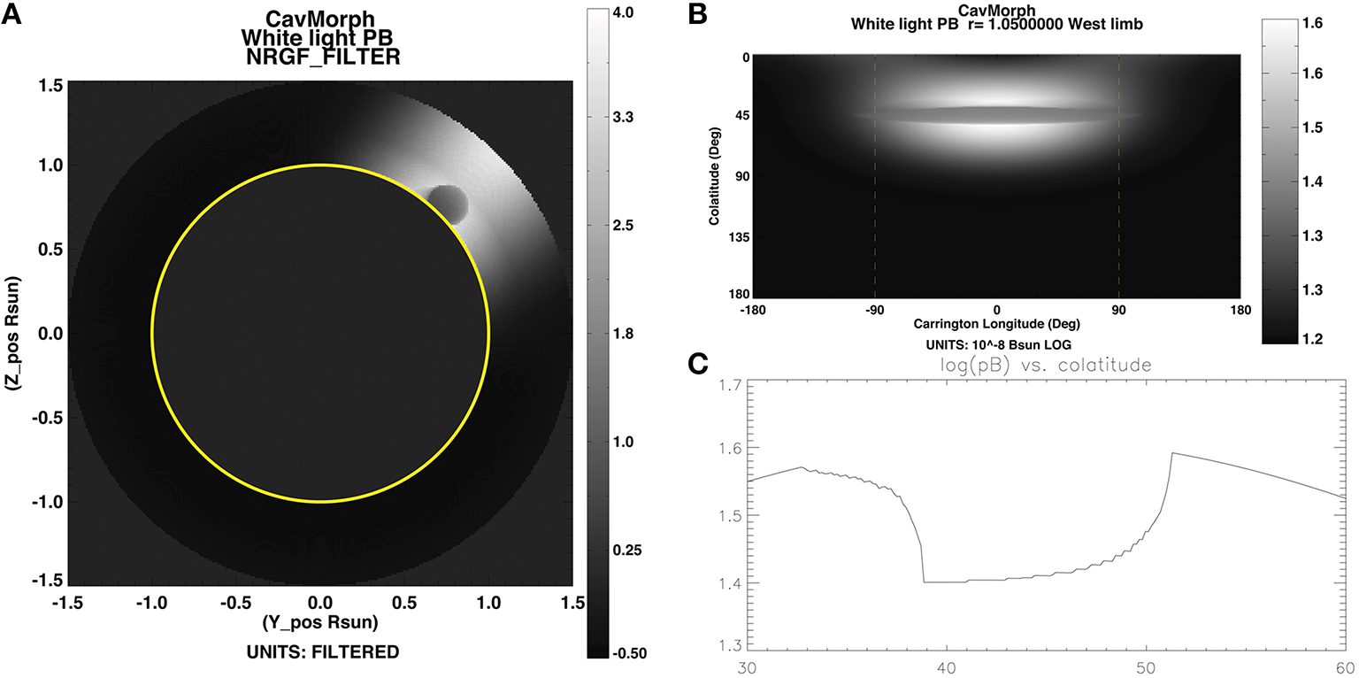
Examples of FORWARD output of LOS-integrated white-light polarized Brightness (pB) for a morphological model of a cavity embedded in a coronal streamer (Gibson et al., 2010). (A) Cavity in plane of sky at limb (plotted with non-radial gradient filter Morgan et al., 2006). Plot obtained by FORWARD line command: for_drive,'cavmorph',inst='wl',line='pb',thcs=45,cavlength=150,rfilter='NRGF_FILTER'. (B) Cavity in latitude-longitude Carrington map. Plot obtained as for (A), but without rfilter keyword and with ,gridtype='Carrmap',cmer=0,charsize=.85 added. (C) Cavity in constant radius latitudinal cut. Plot obtained as for (A), but with removal of rfilter keyword and addition of keywords: ,gridtype='user',ruser=dblarr(201)+ 1.05,thuser=dindgen(201)*.15+30,phuser=dblarr(201)-30.,quantmap=quantmap and followed by command: plot,dindgen(201)*.15+30, alog10(quantmap.data),yrange=[1.3,1.7],xrange=[30.,60.],title='log(pB) vs.colatitude'. Note that this and other IDL commands provided in figure captions below can be accessed via $FORWARD_DOCS/EXAMPLES/examples_forwardpaper.html.
This paper describes how FORWARD addresses all three of the requirements for coronal magnetometric inverson and gives examples of how it may be used. Section 2 demonstrates how the physical state may be defined through analytic or numerical models, either user-inputted or generated by FORWARD through included codes or via its interface with online coronal simulations. Section 3 describes the multiwavelength forward calculations that predict observational manifestations of physical processes such as Thomson scattering, collisional excitation, continuum absorption, resonance scattering, Zeeman and Hanle effects, Doppler shift, thermal bremstrahllung, gyroresonance, and Faraday rotation, and discusses the magnetic diagnostic potential of each. Section 4 describes how FORWARD enables the access and manipulation of observations and converts them to a format directly comparable to the predictions of forward calculations. Section 5 shows how FORWARD may be applied to validate models, build intuition regarding coronal magnetic signatures, tune models to match data, and generally guide the development of multiwavelength magnetometric inversion techniques. Finally, in Section 6 we present our conclusions.
2. The physical state
When discussing solar-coronal forward analysis, it is important to differentiate between the model of the physical state of the corona, which addresses the distribution of magnetic fields and plasma throughout 3D space, and the model of how these fields and plasma operate in the presence of a physical process, which enables the synthesis of an observed quantity. We will treat the latter in Section 3 as the heart of the forward calculation.
Models of the physical state essentially create synthetic Suns—generally through solutions of the MHD equations. FORWARD includes several analytic models in its distribution (i.e., Low and Hundhausen, 1995; Lites and Low, 1997; Gibson et al., 2010; Figure 1; Gibson and Low, 1998; Figure 2). It is straightforward to expand it to incorporate other analytic models. Alternatively, a user may input a numerical data cube describing the 3D distribution of plasma and fields. If the data cube is not global, options are provided regarding what to do outside the cube (e.g., zero, constant, or dipolar field, and hydrostatic atmospheres—either isothermal-exponential or power-law). If the data cube only provides a magnetic field, hydrostatic atmospheres can be applied throughout space. (See http://www.hao.ucar.edu/FORWARD/FOR_SSW/idl/MODELS/NUMCUBE/make_my_cube.pro for instructions on how to convert a numerical data cube to FORWARD format.) In addition to the forward-calculated observables discussed in Section 3, FORWARD allows easy display of the parameters of the physical state, e.g., density, temperature, magnetic field, velocity (see e.g., Figure 2).
Figure 2

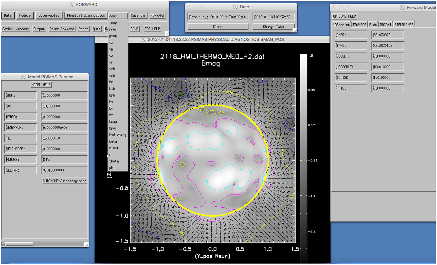
Example of analytic model of a spheromak flux rope embedded in an otherwise open bipolar global magnetic field (Gibson and Low, 1998), provided within the FORWARD distribution and demonstrated here using the for_widget interface. The user chooses the model via the drop-down menu in the top-left widget as shown, and then may choose model parameters (bottom-left widget), and display (as in line-of-sight magnetic field example shown here) model diagnostics (top-left widget, drop-down menu for Physical Diagnostics) with various plotting choices such as plane-of-sky field lines (white vectors; set in right widget). Doing an actual forward calculation of a coronal observable (not shown) is done by choosing one of the Observables (top-left widget, drop-down menu). All calculations are intitiated by clicking on the FORWARD button (top-left widget).
Given a calendar date, FORWARD can also automatically interface with the SolarSoft Potential Field Source Surface (PFSS) package (http://www.lmsal.com/~derosa/pfsspack/) and the web-served Magnetohydrodynamic Algorithm outside a Sphere (MAS)-corona MHD simulation data cubes (http://www.predsci.com/hmi/data_access.php; Figure 3; Lionello et al., 2009). This enables global descriptions of the 3D coronal magnetic field, and for the MAS model also the plasma in MHD force balance, specific to a given time/day and viewer position.
Figure 3
Example of MAS model data cube loaded into FORWARD by date, and displaying magnetic field strength (contours) and field lines (black arrows) in the plane of the sky. As with the analytic model of Figure 2, display options and model parameters can be set through the widgets. Descriptions of the model parameters and other options are found via the TOP HELP, MODEL HELP, and OPTIONS HELP buttons at the top of the three main widget windows. See Section 3 for further discussion and Figures 4, 6 for examples of forward calculation using the MAS and PFSS models.
FORWARD also allows the user to specify the physical state of two populations of plasma that may need to be treated independently in the forward calculation. For example, a user may specify a population of plasma at a coronal temperature, and another population of cooler, chromospheric plasma subject to continuum absorption in EUV images (see Section 3.3). This provides capability, for example, for depicting models where cool solar prominences exist in the context of surrounding coronal temperature material, such as those produced by Luna et al. (2012) or Xia et al. (2014) (see also the cavity-prominence test-bed simulation shown in Section 5). Another application would be to allow models where two different coronal populations lie along the line of sight, each with different abundance properties. It is also possible to set a filling factor for one or both populations. This capability allows exploitation of the diagnostic potential of comparing emissions which may have different dependencies on density (as we discuss in Section 3).
3. The forward calculation: physical processes
Given a modeled physical state, i.e., a specification of the distribution of density, temperature, magnetic field and velocity in the corona, FORWARD is able to produce many different synthetic observables. These observables arise from various physical processes manifesting at different wavelengths of light in the corona. They depend upon the viewer's line of sight, along which (for example) optically-thin emission must be integrated. FORWARD establishes these lines of sight either through keyword definition of an observer's heliographic latitude and longitude, or through keyword setting of a calendar date from which the position of the Earth (or STEREO spacecraft) can be determined. In this section, we will discuss a range of physical processes relevant to the corona, describe how they translate to observables that FORWARD synthesizes, and consider their potential for coronal magnetometry. Table 1 provides a summary.
Table 1
| Process | Physical-state dependency | Observation | Magnetic quantity probed |
|---|---|---|---|
| Thomson scattering | Electron density | White-light pB, TB | Plasma structured by field (e.g., closed vs. open field boundaries, flux surfaces) |
| Collisional excitation | Electron density, temperature | IR/Visible/EUV/SXR emission | Plasma structured by field (incl. loops, closed/open boundaries, flux surfaces) |
| Continuum absorption | Chromospheric population density, electron density, temperature | EUV absorption features | Can indicate magnetic geometry suitable for prominence formation |
| Resonance scattering; polarization | Electron density, temperature, vector magnetic field | Visible/IR spectra | Blos from Stokes V; Magnetic field direction from Stokes Q, U |
| Doppler shift | Electron density, temperature, velocity | Visible/IR spectra | Bpos and field line direction from waves; flux surfaces from bulk flows |
| Thermal bremstrahllung | Electron density, temperature, vector magnetic field | Radio emission (intensity and circular polarization) as a function of frequency | Blos from Stokes V |
| Gyroresonance | Electron density, temperature, vector magnetic field | Radio emission (intensity and circular polarization) as a function of frequency | Surfaces of constant magnetic field strength at each frequency |
| Faraday rotation | Electron density, temperature, vector magnetic field | Rotation of plane of polarization | Blos from rotation measure |
Physical processes as defined in Section 3, highlighting dependency on attributes of the physical state, which observations are sensitive to them, and diagnostic sensitivity to the 3D coronal magnetic field.
3.1. Thomson scattering
Thomson scattering is the main physical process responsible for illuminating the continuum, or “K” corona. Photospheric light scatters off of free coronal electrons and results in both unpolarized and linearly polarized emission. Both the total brightness (TB) and polarized brightness (pB) of white light are proportional to ne and to a scattering function that depends upon radial distance from the photosphere (Billings, 1966). They are also integrated along the line of sight in the optically-thin corona.
Given a distribution of electron density, FORWARD can synthesize images of TB, pB, and degree of polarization p (Figures 4A, 5A), comparable to observations from white light coronagraphs such as SOHO/LASCO, STEREO/SECCHI, and MLSO/KCOR. If keyword fcor is set, FORWARD will call upon SolarSoft function fcorpol_KL.pro in order to add a model distribution of F-coronal brightness (Koutchmy and Lamy, 1985). This arises from light diffracting through interplanetary particles in the plane of the ecliptic, and is also known as the zodiacal light. It is essentially unpolarized in the first few solar radii (Mann, 1992).
Figure 4
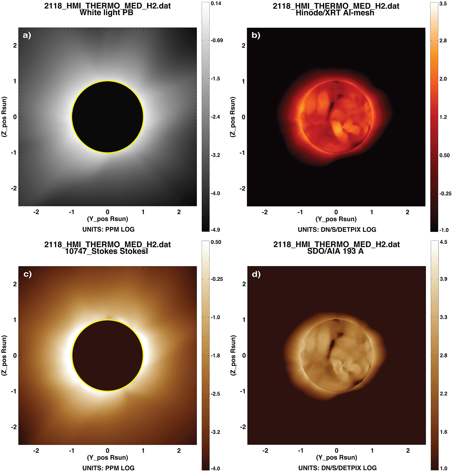
Figure showing MAS synthetic data. (A) pB (see Section 3.1). Plot obtained via widget as in Figure 2 but selecting pB via the Observables menu, or alternatively via FORWARD line command for_drive,'psimas',date='2012-01-04',xxmin=-2.5,xxmax=2.5,yymin=-2.5,yymax=2.5, units='PPM'. (B) XRT Al-Mesh line (see Section 3.2). Plot obtained as in (A) with removal of units keyword and addition of /xrt,line='AL-MESH', usecolor=3. (C) (infrared) Fe XIII 1074.7 Å intensity (see Section 3.4). Plot obtained as in (A) with additional keyword /comp,ngrid=256,ngy=256. (D) (EUV) Fe XIII 193 Å intensity (see Section 3.2). Plot obtained as in (A) with removal of units keyword and addition of /aia. Note that (A,C) are in units of 10−6 solar Brightness (log), or parts per million (PPM). (B,D) are in instrument detector units per second with default intensity ranges chosen to match expectations of XRT and AIA telescopes.
Figure 5
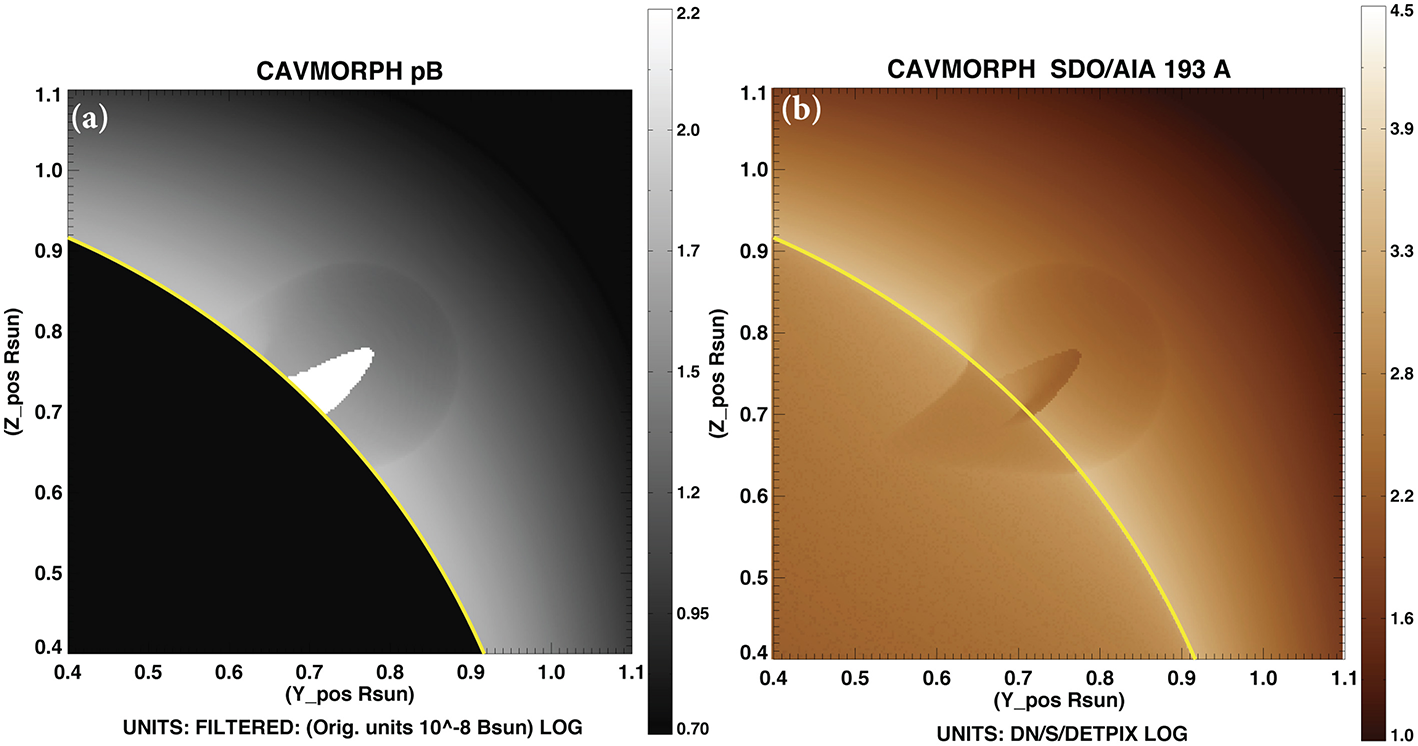
A simplified cavity and prominence produced using the Gibson et al. (2010) model. (A) synthesized white light polarized brightness (see Section 3.1), with high-density prominence appearing as enhanced intensity. Plot obtained by FORWARD line command: for_drive, 'cavmorph',/nougat,thcs=45,cdens=1e10,cff_noug=[.2,8.,0,0,0,0],nougwidth=.025,nougtop_r=.9,pop2T=2,xxmin=0.4,yymin=0.4,yymax=1.1, xxmax=1.1.(B) SDO/AIA 193 Å emission, with dark prominence because of continuum absorption (see Sections 3.2–3.3). Plot obtained by above command with the addition of keyword /aia.
Thomson scattering has no direct dependency on magnetic field, but there is sensitivity to magnetic topology through its dependence on density. For example, bright (dense) coronal streamers generally correspond to closed magnetic fields, and dark (sparse) coronal holes generally correspond to open magnetic fields. For this reason, white light coronagraph data have been used to qualitatively validate features of coronal magnetic models (Newkirk and Altschuler, 1970), and more quantitatively, to define the average nonradial expansion of magnetic fields in coronal holes (Kopp and Holzer, 1976; Munro and Jackson, 1977). Magnetic flux surfaces also may be delineated by white light structures, such as three-part CME features (Low and Hundhausen, 1995), and prominence cavities (e.g., Figure 5A; see also Gibson and Fan, 2006).
3.2. Collisional excitation
Solar coronal radiation in the extreme ultraviolet (EUV) and soft X-ray (SXR) is produced by collisionally-excited atoms in thermal and ionization equilibrium. The intensity of this emission is proportional to and the temperature response of the line(s). For spectrographs, FORWARD calculates the integrated intensities of lines in physical units to be compared with processed spectral data. For waveband imagers, FORWARD incorporates the wavelength-response function of the instrument into its calculated intensities. The emission is integrated along the line of sight in the optically-thin corona.
FORWARD synthesizes images comparable to those produced by numerous EUV and Soft X-ray imagers and also many spectral line intensities in these wave bands. Currently simulated imagers include SOHO/EIT, STEREO/EUVI, Hinode/XRT (e.g., Figure 4B), ProbA-2/SWAP, and SDO/AIA (e.g., Figures 4D, 5B). Adding new imagers is straightforward if the wavelength response function is available. Count rates for imagers are calculated by convolving the wavelength response function of the imager with pre-calculated spectra at various temperatures and densities, produced using the Chianti atomic data base and related software (Dere et al., 1997; Del Zanna et al., 2015). For the imagers, users may select from pre-calculated abundance options; current selections include coronal abundances determined by Feldman et al. (1992) or Schmelz et al. (2012) or photospheric abundances of Caffau et al. (2011). The code uses the Chianti ionization equilibrium calculations (Dere et al., 2009).
Spectral line intensities can be calculated for any line between 1 and 1410 Å, again under the assumption that the coronal plasma is collisionally excited and in thermal and ionization equilibrium. Based on a user-specified instrumental line-width, the code includes any blended lines included in the Chianti spectral line calculations. For spectral lines, users may specify any abundance or ionization table in the Chianti database format. Default line widths are provided for particular instruments like Hinode/EIS, IRIS, and SoHO/CDS, but the code is not limited to lines observed by these instrument. The wavelength range covers the IRIS far ultraviolet (FUV) range, but not the near ultraviolet (NUV) range, which does not include lines that can be modeled by FORWARD.
As with Thomson scattering, radiation from collisional excitation does not have a direct dependence on magnetic fields. However, the suppression of conductivity across magnetic field lines means that magnetic field lines are essentially traced out in coronal emission. EUV and SXR structures thus often provide a diagnostic of local magnetic field geometry—for example when coronal loops are lit up in active regions (see e.g., Savcheva et al., 2013; Malanushenko et al., 2014; also Savcheva and Malanushenko, in preparation). Magnetic boundaries or flux surfaces are also often delineated due to sharp density/temperature gradients, as in the case of open vs. closed fields (e.g., Figures 4B,D), and prominence cavities (e.g., Figure 5B).
3.3. Continuum absorption
Relatively cool, chromospheric temperature material suspended in the corona (e.g., a prominence) results in Lyman continuum absorption by neutral hydrogen and by neutral and once-ionized helium (see Kucera, 2015 for further details).
The observed intensity is where If is the foreground radiation, Ib is the background radiation, and τ is the continuum absorption summed over the three absorbing species: where h is the distance along the line of sight, ni is the number density of each species, and σi is the absorbing cross section as a function of wavelength (values calculated with the formulation of Keady and Kilcrease, 2000).
Through the definition of a second population of low-temperature plasma with a specified density distinct from the primary coronal population, FORWARD calculates the effect of continuum absorption on the total intensity in EUV. Figure 5B shows a model of a simple prominence inside a cavity in the 193 Å band of SDO/AIA. The cavity is darker than its surroundings because it has a lower density, but the central prominence is darker because of continuum absorption of background emission.
Again, continuum absorption has no direct dependence on magnetic fields. However, magnetic field geometry (e.g., dipped or flat field lines) is expected to play an important role in establishing where prominences form (see Karpen, 2014 and references therein).
3.4. Resonance scattering and polarization
Emission from the coronal forbidden lines arises both from collisional excitation as described above in Section 3.2, and also from resonance scattering. In resonance scattering, anisotropic radiation from the underlying photosphere excites coronal ions and leads to reemitted light with a characteristic polarization signature (Casini and Judge, 1999). This emission depends linearly upon ion density (and thus electron density), as opposed to quadratically as in collisional excitation. Figure 4C vs. Figure 4D illustrates the difference between the collisionally-excited/resonantly-scattered infrared Fe XIII line and the predominantly collisionally-excited EUV Fe XIII line. Intensity of the latter drops off quickly, while the former shows similarity in the outer field of view to the Thomson-scattered white light (Figure 4A), which is also linearly-dependent upon electron density at these heights (see Habbal et al., 2011 for further discussion).
FORWARD employs the Coronal Line Emission (CLE) Fortran-77 polarimetry code developed by Judge and Casini (2001) to synthesize Stokes (I, Q, U, V) line profiles for the visible and infrared forbidden lines including Fe XIII 1074.7 and 1079.8 nm (currently observed by MLSO/CoMP as discussed in Section 4), Fe XIV 530.3 nm, Si IX 393.4 nm, and Si X 1430.5 nm. Stokes I indicates the total intensity of the line, Q and U together constitute its linearly polarized intensity, and V is the circularly polarized intensity. The CLE code models the lines under the combined influence of resonance scattering and particle collisions in the presence of coronal magnetic fields.
Because of its sensitivity to magnetic fields, the Stokes I, Q, U, V polarization vector can be used as a direct diagnostic of coronal magnetism (subject to intensity-weighted line-of-sight integration). For example, the Zeeman effect generates circularly polarized light (Stokes V) proportional to line-of-sight-oriented magnetic field Blos. Since the coronal visible/infrared forbidden lines treated by CLE have a Larmor frequency νL ≈ μBB/h that is much larger than the inverse lifetime of the atomic transitions being modeled, they lie in the strong field (or saturation) limit of the Hanle effect (see Raouafi et al., submitted; Dima et al., submitted) for discussion of magnetometry in the UV “unsaturated” Hanle regime). In the saturated regime, linear polarization provides a probe of the direction of the magnetic field in the plane-of-sky (POS), but not its strength. In particular, the direction of the linear polarization vector [or azimuth, Az = −0.5 ∗ atan(U/Q)] is parallel to the POS component of the magnetic field, as long as the local magnetic vector field has an angle relative to the solar radial direction (ϑB) less than the critical “van Vleck” angle, at which point the azimuth becomes perpendicular to the POS field. This occurs because the atomic alignment upon which the linear polarization depends goes through zero (and changes sign) when , i.e., when (van Vleck, 1925). The location of van Vleck nulls in linear polarization thus also acts as a diagnostic of magnetic field direction (see Section 5.1 for further discussion).
Figures 6A,C,E,G shows I, V/I, Az and L/I calculated from the MAS coronal model. From this it is clear that, despite the line-of-sight superposition of optically-thin coronal plasma, Stokes polarimetry can provide a quantitative measure of coronal magnetic field strength and direction. The Stokes V/I (Figure 6C) represents a line-of-sight intensity-weighted average of Blos. The dark linear-polarization features shown in Figure 6E) are generally signatures of magnetic fields oriented at the van Vleck angle (although note that the presence of strong Blos field can also result in linear polarization nulls; see Section 5.1 for further discussion). Even with LOS integration, the linear polarization vectors (blue) are largely aligned with the POS magnetic field vectors (red) (see Figures 6A,E), except when at the van Vleck angle they flip 90°. Figure 6G) also illustrates this sensitivity to POS magnetic field direction, showing magnitude of departure from radial-orientation in Az (red = counterclockwise, blue = clockwise). The coronal hole in the south/southwest is evident as a broad blue/red interface in Az, indicative of diverging magnetic fields, while closed field structures exhibit a red-black-blue interface (e.g., south/southeast) which indicates converging fields.
Figure 6
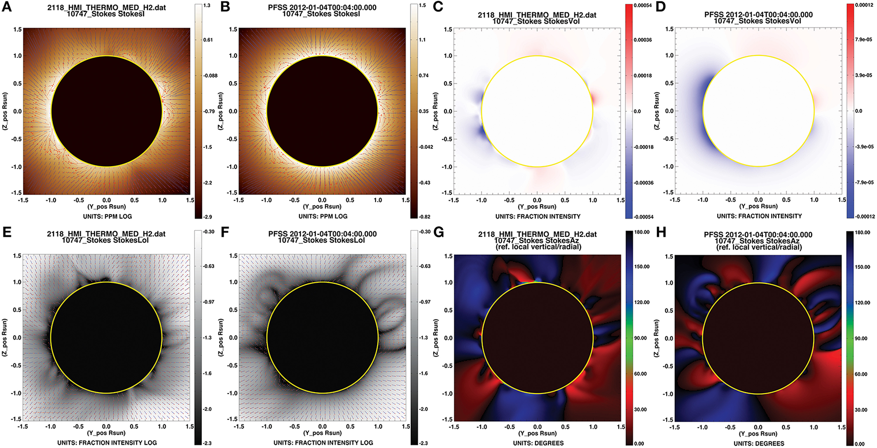
Synthetic polarimetric data from MAS (A,C,E) and PFSS (B,D,F) models. (A,B) Intensity of Fe XIII 1074.7 Å infrared line, with POS magnetic vectors (red) and linear polarization vectors (blue). Plot for (A) obtained in a similar manner as Figure 2, i.e., for_drive,'psimas',date='2012-01-04',ngrid=256, ngy=256,/comp,/fieldlines,/stklines,/savemap,mapname='psimas_10747_01042012'. The savemap keyword creates an IDL save set (used in plots to follow) which contains information of the full Stokes vector. (C,D) Percent circular polarization V/I. Plot for (C) obtained by for_drive,readmap= psimas_10747_01042012',line='VoI'. (E,F) Percent linear polarization L/I, with magnetic and linear polarization vectors (length not scaled by magnitude). Plot for (E) obtained as for V/I but with line='LoI' set, and additional keywords, /fieldlines,bscale=-.6,/stklines,pscale=-.2. (G,H) Direction Az of linear polarization vector in local vertical (radial) reference frame. Plot for (G) obtained as for V/I but with line='Az' set. Plots for (B,D,F,H) are obtained as for (A,C,E,G), substituting pfss for psimas.
Strongly nonradial azimuths (represented as green in the local-vertical reference frame of Figure 6G) are rare. They can occur if the local magnetic vector >54.74° as measured from the solar radial direction but the POS projection is close to radial, as in the case of magnetic fields that are oriented largely along the LOS. In order for such a nearly-perpendicular azimuth to survive LOS integration, either the plasma must be localized to a magnetic structure oriented in this manner, or a larger-scale magnetic structure must possess a symmetry along the LOS. Such symmetries are fairly common in large-scale POS-oriented fields extended along the LOS, e.g., arcade fields or coronal holes, and because such structures are POS-oriented, they possess a strong linear-polarization signal and so the azimuth survives LOS integration (see further discussion in Section 5.1). Even if LOS-oriented fields are localized or exist with orientation extended along the LOS, however, because they do not possess a strong linear polarization signal they are likely to be obscured by any POS-oriented fields lying along their integration path.
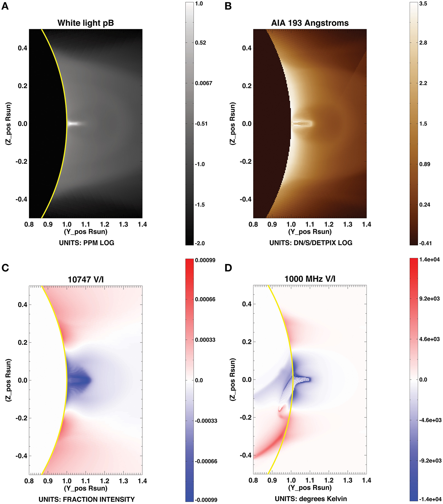
Figures 6B,D,F,H shows the polarization for a potential field model extrapolation for the same day and using similar (although not identical) photospheric magnetic boundary data as the MAS model of Figures 6A,C,E,G. The differences between MAS and PFSS predictions for circular and linear polarization result from differences at the lower boundary, from the non-potentiality of the MAS model magnetic field, and also to some degree from differences in intensity-weighting along the line of sight (the PFSS solution requires a density/temperature distribution that is spherically-symmetric). The significance of intensity weighting is also evident in Figure 7, where the LOS-integrated Stokes V differs depending on the wavelength used to observe it (visible, IR, radio). Since the same (MAS) model is used for all four forward calculations, variation must be due to the different sensitivities to temperature and density for the four wavelength regimes, which in turn means that different distributions of plasma are contributing to the integrals along the line of sight. In Section 5 we will discuss the importance of making full use of such multiwavelength magnetic dependencies in choosing between models.
Figure 7
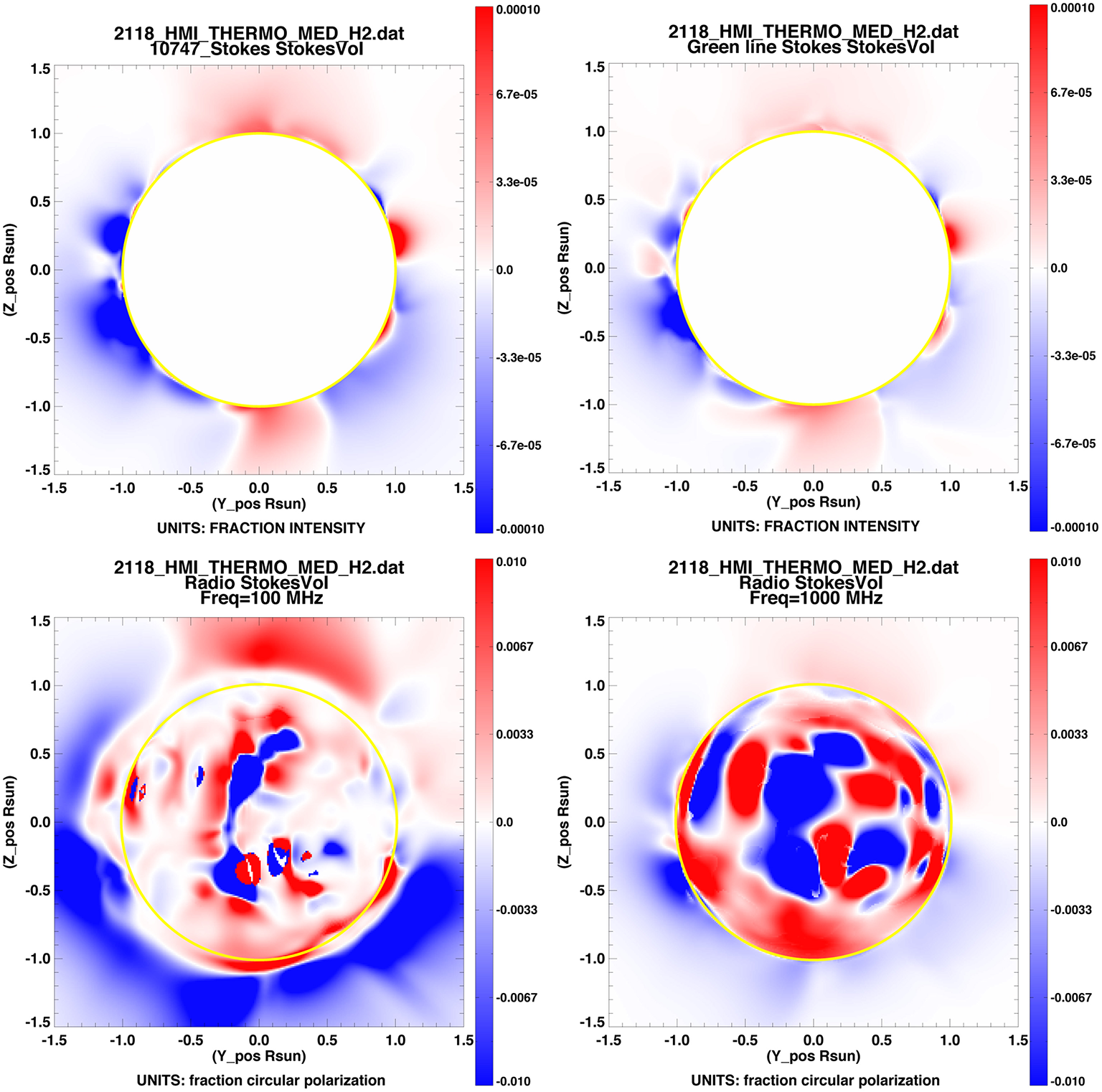
Because of different dependencies on plasma along the line of sight, the representation of integrated circular polarization (dependent upon line-of-sight magnetic field strength) appears differently at different wavelengths. (Top left) MAS model V/I for Fe XIII 1074.7. Plot obtained as in Figure 6, with additional keywards imin=-0.00001,imax=0.00001. (Top right) Same for Fe XIV green line. Plot obtained by following the process outlined in Figure 6, but substituting /greencomp for /comp. (Bottom left) Same for radio bremstrahllung, at a frequency of 100 MHz. Plot obtained as in Figure 6, but with /radio instead of /comp and frequency_MHz=100,imin=-0.001,imax=0.001. (Bottom right) Same, but substituting frequency_MHz=1000. Unlike the visible and IR lines, radio frequencies can be observed above the solar disk as well as at the limb.
3.5. Doppler shift
If light-emitting plasma is moving, spectral lines are subject to a Doppler shift proportional to the line-of-sight component of the plasma velocity (vlos). For optically-thin plasma, this vlos is further weighted by the distribution of intensity along the line of sight. From the line profiles in the visible and IR generated by CLE (see Section 3.4), FORWARD determines Doppler shift and integrates along the line of sight to get a synthetic observable comparable to observations.
Doppler velocity observations in the IR by the MLSO/CoMP telescope have proved to be a good resource for measuring ubiquitous waves in the corona (Tomczyk et al., 2007). The phase speeds of these waves are expected to be proportional to the plane-of-sky component of the magnetic field strength, and the direction of propagation of the waves will be aligned with the magnetic field direction. In general, the flux-freezing condition forces plasma flows to follow the direction of the magnetic field, so bulk velocity flows also can act as a probe of magnetic structure (Figure 10C; Ba̧k-Stȩślicka et al., 2013, also Ba̧k-Stȩślicka et al., submitted).
3.6. Radio emission: thermal bremstrahllung and gyroresonance
The two thermal emission mechanisms that dominate non–flaring solar radio emission are bremsstrahlung (also known as “free–free emission”) and gyroresonance emission. Bremsstrahlung is produced by all plasma in the solar atmosphere and is strongest in dense regions, while gyroresonance emission requires strong magnetic fields in the corona and is usually confined to locations above sunspots. The Jansky Very Large Array, the Expanded Owens Valley Solar Array, the Nobeyama Radioheliograph and the Mingantu Ultrawide Spectral Radioheliograph are examples of radio telescopes capable of high-resolution, high-dynamic-range imaging, including circular polarization imaging, in the frequency range (1–20 GHz) where these two mechanisms are important diagnostics of the magnetic field in the solar atmosphere.
Optical depths are generally significant in the solar atmosphere at radio wavelengths and in order to calculate the radio emission arising from either of these physical processes one must carry out a radiative transfer calculation (as for continuum absorption in Section 3.3). It is convenient to do the calculation in terms of brightness temperature, TB, because radio emission takes place in the Rayleigh–Jeans limit where the effective radiative temperature of an optically thick source is the physical temperature of that source. Brightness temperature may be converted to flux density S via the relation where kB is Boltzmann's constant, c is the speed of light and the integral is over the solid angle Ω of interest. Note that brightness temperature is a local quantity whereas flux density is integrated over a source area.
The radiative transfer calculation for radio emission in FORWARD follows standard methods: the brightness temperature transfer is governed by the differential equation (e.g., Dulk, 1985): where κ is the opacity per unit distance s along the line of sight and Te is the local electron temperature. We solve radiative transfer by determining κ and Te in each pixel along the line of sight and integrate Equation 4 across each pixel as follows: where TB is the incident brightness temperature, and is the emergent brightness temperature—integrated across the line-of-sight pixel and serving as the incident brightness temperature to the next pixel. dτ = κds is the opacity change across the pixel.
Radio emission from the solar atmosphere is strongly influenced by the magnetic field in the emitting regions and provides valuable diagnostics of solar magnetic fields that complement other techniques. The magnetic field plays a role in the absorption coefficients κ: electrons interact more strongly with the sense of circular polarization that matches the sense of rotation of an electron as it spirals along magnetic field lines under Larmor motion. The polarization that interacts more strongly with electrons is the extraordinary or x mode, with the other polarization being labeled the ordinary (o) mode. Under most conditions in the solar corona, and following propagation to terrestrial observers, the x and o modes are 100% circularly polarized with opposite sense of polarization. FORWARD solves the radiative transfer equations as described above for each of the circular polarizations separately. The difference between the x and o modes is then Stokes V (modulo a sign), while the sum is the total intensity, Stokes I (For radio emission from the solar atmosphere, we may ignore any weak linear polarization present due to the fact that the large Faraday rotation in the solar atmosphere wipes out linear polarization over a finite observing bandwidth, see below).
For thermal bremsstrahlung, which is always included in a FORWARD radio emission calculation, opacity results from collisions between electrons and ions. We use the simple expression (Dulk, 1985; Gelfreikh, 2004) which is appropriate for coronal temperatures, where Hz is the electron gyrofrequency and the factor in parentheses deals with polarization (with the assumption that f ≫ fB): θ is the angle between the magnetic field direction and the line of sight, and the minus sign refers to the x mode while the plus sign refers to the o mode. Thus, the magnetic field information present in bremsstrahlung emission resides in the circular polarization and represents the line-of-sight component of B.
The dependencies in Equation 6 mean that bremsstrahlung is strongly favored in dense regions of the atmosphere and weighted toward cooler material (since in Equation 4, , e.g., White, 2000). The f−2 dependence of bremsstrahlung opacity also means that optical depth decreases rapidly as frequency increases, and at low frequencies one is likely to be optically thick such that the lower the frequency, the higher in the atmosphere one sees. This is evident in Figure 8, where polarization extends much higher above the photosphere at 100 MHz (lower left panel) than at 1000 MHz (lower right panel). When optically thick, the circular polarization produced by bremsstrahlung emission actually depends on the presence of a temperature gradient. If one has well–calibrated brightness temperature measurements across a continuous frequency range, one can in fact determine both the temperature gradient and the magnetic field from the data (Grebinskij et al., 2000, disproving a comment in White, 2000). In Figure 7 the lower degrees of polarization over much of the disk at 100 MHz reflect the fact that the temperature gradient is weaker higher in the corona.
The gyroresonance calculation is more complex. Gyroresonance opacity results from the acceleration of electrons in a magnetic field under the Lorentz force, and is only significant in narrow layers where the observing frequency f is a low integer multiple s of the electron gyrorequency fB (e.g., White and Kundu, 1997). The optical depth τ of a thermal gyroresonance layer (the absorption coefficient integrated through the layer) is where LB(θ) is the scale length of the magnetic field () evaluated along the line of sight and . For coronal conditions μ ≈ 2000, and the μ−s dependence in Equation 7 produces a dramatic change in opacity as harmonic number s changes. Fx, o(θ) is a function of angle which is of order unity for the x mode near θ = 90°, but decreases sharply at smaller θ, and is smaller in the o mode than in the x mode. FORWARD uses a more exact approximation for τx, o due to Robinson and Melrose (1984) which requires a careful calculation of the cold plasma properties of the electromagnetic modes under the conditions that apply in the gyroresonance layer. FORWARD incorporates gyroresonance emission by testing for harmonic layer crossings along the line of sight in the range s = 1 to 5, and calculating the resulting opacity as shown above: significant gyroresonance opacity at higher harmonics generally requires mildly relativistic electrons which puts emission in the gyrosynchrotron limit in which harmonics are much broader and Equation 7 is no longer valid [Note the simulation package GX_Simulator can handle gyrosynchrotron emission (Nita et al., 2015)].
Gyroresonance emission is most commonly seen in the strong magnetic fields above solar active regions. At frequencies above a few GHz, bremsstrahlung does not produce enough opacity to make the corona optically thick, while the large change in gyroresonance opacity as s decreases (typically a factor of order 1000) means that a given harmonic layer is usually either very optically thick or very optically thin. When optically thick, gyroresonance produces million-K coronal brightness temperature features in radio images. In practice, we see down to the highest optically thick layer (usually s = 3 in x mode and s = 2 in o mode), and the brightness temperature variations across the surface (of constant field strength for a given frequency) represent actual temperature variations across that surface. Thus, for this mechanism the magnetic field information contained in the emission morphology is somewhat complex and does not simply reside in the polarization (White and Kundu, 1997).
Internally, FORWARD carries out radiative transfer for radio emission in the x and o modes by summing the requested absorption coefficients in each pixel: bremsstrahlung is the default opacity and gyroresonance opacity may be turned on or off. The brightness temperatures in the two modes are summed and differenced to report Stokes I and V, or one can display V/I, the degree of circular polarization, as in Figures 7, 8. Mode coupling between the x and o modes, which can result in reversal in the sense of circular polarization at points where the magnetic field direction along the line of sight reverses (e.g., White et al., 1992), is not yet included in the FORWARD calculation but will be in future releases. Figure 8 shows an example of a FORWARD radio emission calculation using a three–dimensional hydrodynamic active region model (density, vector magnetic field and temperature) with thermal conduction and radiative cooling (Lionello et al., 2013). The upper panels show the model radio emission obtained with just bremsstrahlung opacity included, while the lower panels include gyroresonance opacity. The brightness temperatures are much higher when gyroresonance opacity is included, and the polarization structure becomes more complex.
Figure 8
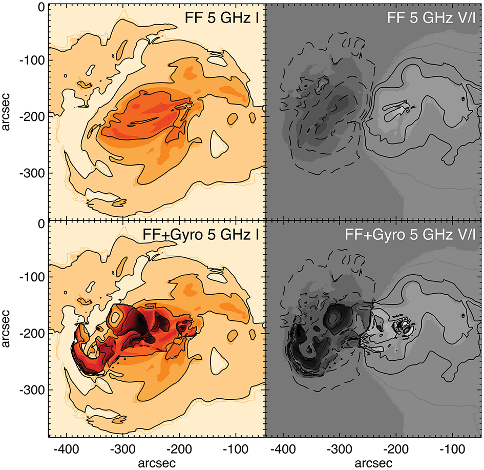
Radio emission from a model active region comparing calculations with and without gyroresonance emission. Thermal bremstrahllung or free–free emission (“FF”) is included in both cases. Total intensity (Stokes I) is plotted in the left panels and degree of polarization (V/I, scaled from −1 to 1) is plotted in the grayscale in the right panels, with contours showing Stokes V. The brightness temperature display range in the left–hand panels is 0 to 2.5 × 10⁶ K. Contour levels are at 16, 32, 64, 128, and 256 × 104 K in the Stokes I panels, and 1, 4, 16, and 64 × 104 K in the V/I images. The pixel size is 1.5 arcsec.
FORWARD does not currently include plasma emission: this is the dominant emission in low–frequency solar radio bursts (e.g., Kundu, 1965), but it is a coherent emission mechanism and there is no simple way to calculate it (e.g., see Schmidt and Cairns, 2012a,b, for a detailed calculation). In addition, fundamental plasma emission occurs at frequencies where the refractive index may be significantly different from unity and refraction can play a major role in determining ray paths. FORWARD assumes linear ray paths along lines of sight and does not currently handle refraction at low radio frequencies which will produce curved ray paths in a realistic solar atmosphere.
3.7. Faraday rotation
In general radio emission can be elliptically polarized. Electromagnetic radiation in a magnetized plasma can be decomposed into two natural modes with orthogonal polarizations, and as radiation propagates the two intrinsic polarizations have different refractive indices and slightly different phase speeds. This effect causes the plane of linear polarization to rotate, with the amount of rotation being a function of frequency. In the lower regions of the solar atmosphere the rotation is so large that, as mentioned in the previous subsection, when averaged across a finite observing bandwidth the linear polarization is washed out. However, further out in the solar wind where the magnetic field is lower, Faraday rotation can be measured as a function of frequency, and such measurements are one of the few techniques that can be used as a remote probe of the magnetic field in the solar wind. This technique has been applied to both communication transmissions from satellites (e.g., Bird et al., 1985; Jensen et al., 2005, 2013) as well as polarized background cosmic sources (e.g., Bird et al., 1980; Mancuso and Spangler, 2000; Ord et al., 2007; You et al., 2012; Kooi et al., 2014). In FORWARD it can be used to simulate the contributions of CME and solar wind plasma to an observable diagnostic of the magnetic field.
The expression for Faraday rotation is relatively straightforward: the angle of rotation FR (in radians) at wavelength λ is
where the rotation measure RM (measured in radians per square meter) is the wavelength-independent measure of Faraday rotation, calculated from the integral of the product of electron density and line–of–sight magnetic field along the ray path:
with B measured in Gauss and electron density in cm−3. FORWARD carries out this integral and will report either FR at a specific frequency or RM.
A related and useful quantity that is obtained in conjunction with Faraday rotation measurements of pulsars is dispersion measure, which in radio astronomy is usually measured in units of cm−3 parsecs. The dispersion measure is used to remove the frequency-dependent delay of pulsar pulses introduced by the variation of refractive index in the interstellar and interplanetary media with frequency, so that pulses can be aligned across the full observing bandwidth, a necessary step in measuring the rotation of the plane of polarization vs. frequency. FORWARD provides the same quantity but referred to as a column density (accessed via keyword /colden or in the Physical Diagnostics drop-down menu of the widget, in units of cm−2). Variations in DM on timescales of tens of minutes to hours are dominated by density variations in the solar wind, and knowledge of DM is valuable when trying to assess the relative roles of density and magnetic field in observed RM variability.
4. Observations
As described above in Section 3 and summarized in Table 1, multiple physical processes operating in the corona have sensitivities to the coronal magnetic field and manifest observable signatures from radio to soft-Xray emission. There is thus clear value in obtaining observations at a broad range of wavelengths for intercomparison and use in constraining and defining models.
To facilitate model-data comparisons, FORWARD enables the access and manipulation of observations in a form designed to match the output of forward calculations. To this end, FORWARD extracts SolarSoft IDL maps from FITS-format observational data files, and preserves these along with associated structures in a standard format. Observational data are accessed either “by date” or “by file”—via keywords if using the command-line version of FORWARD, or a calendar/directory search if using the widget interface (see Figure 9). Note that FORWARD looks first in a user-defined working directory for existing FORWARD-formatted maps or fits files before downloading or processing new files.
Figure 9
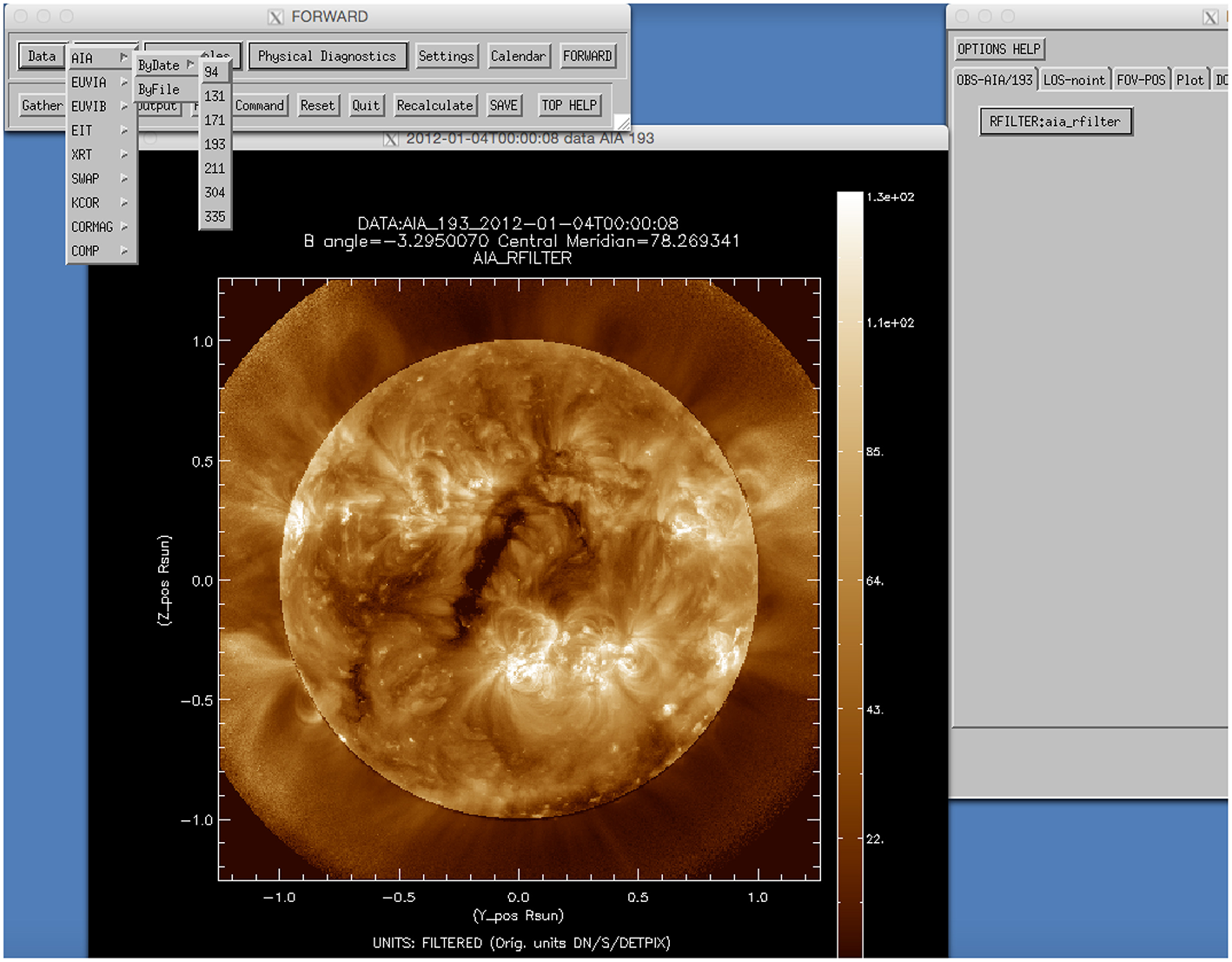
Example of automatically uploading SDO/AIA data via FORWARD widget by date access. Data are accessed via either the Virtual Solar Observatory SolarSoft interface, or an observatory's own web interface. Data may also be uploaded by file from locally stored FITS files, and in some cases (e.g., the CorMag telescope—Fineschi et al., in preparation), this is currently the only available choice.
Since the focus of this paper is magnetometry, we first describe how FORWARD enables access and manipulation of Stokes polarimetric data. The Mauna Loa Solar Observatory (MLSO) Coronal Multi-channel Polarimeter (CoMP) on Hawaii (Tomczyk et al., 2008) is a 20-cm aperture coronagraph with a full field of view of the corona from 1.05 to 1.38 solar radii. It utilizes a narrow-band imaging polarimeter to observe the Fe XIII coronal line at 1074.7 and 1079.8 nm and the chromospheric HeI line at 1083 nm. Data products currently served include intensity, Doppler velocity, line width, and Stokes linear polarization [Q, U as well as L = and ]. CoMP linear polarization is currently the only direct magnetic diagnostic of the corona publicly available on a near-daily basis (subject to weather, etc.). These data are available online, beginning from May 2011, and can be downloaded in FITS or image format via the MLSO web pages (http://www2.hao.ucar.edu/mlso).
FORWARD offers another means of downloading CoMP data, and moreover acts as a tool for its display and analysis (see Gibson, 2015b for further details). Figures 10B,D illustrate FORWARD linear polarization output given a specified calendar date and field of view. In this case, CoMP standard “Quick Invert” data file for that date is automatically accessed, which represents an averaged image and may not include all CoMP data products. Comprehensive, non-averaged data are available in the “Daily Dynamics” and “Daily Polarization” FITS archives on the MLSO web pages, and once these are downloaded to a local directory they may be displayed “by file” using FORWARD. This has been done to show the CoMP Doppler velocity image of Figure 10C. White light data from the MLSO K-coronagraph (KCOR) can similarly be downloaded and displayed through the FORWARD widget tools.
Figure 10
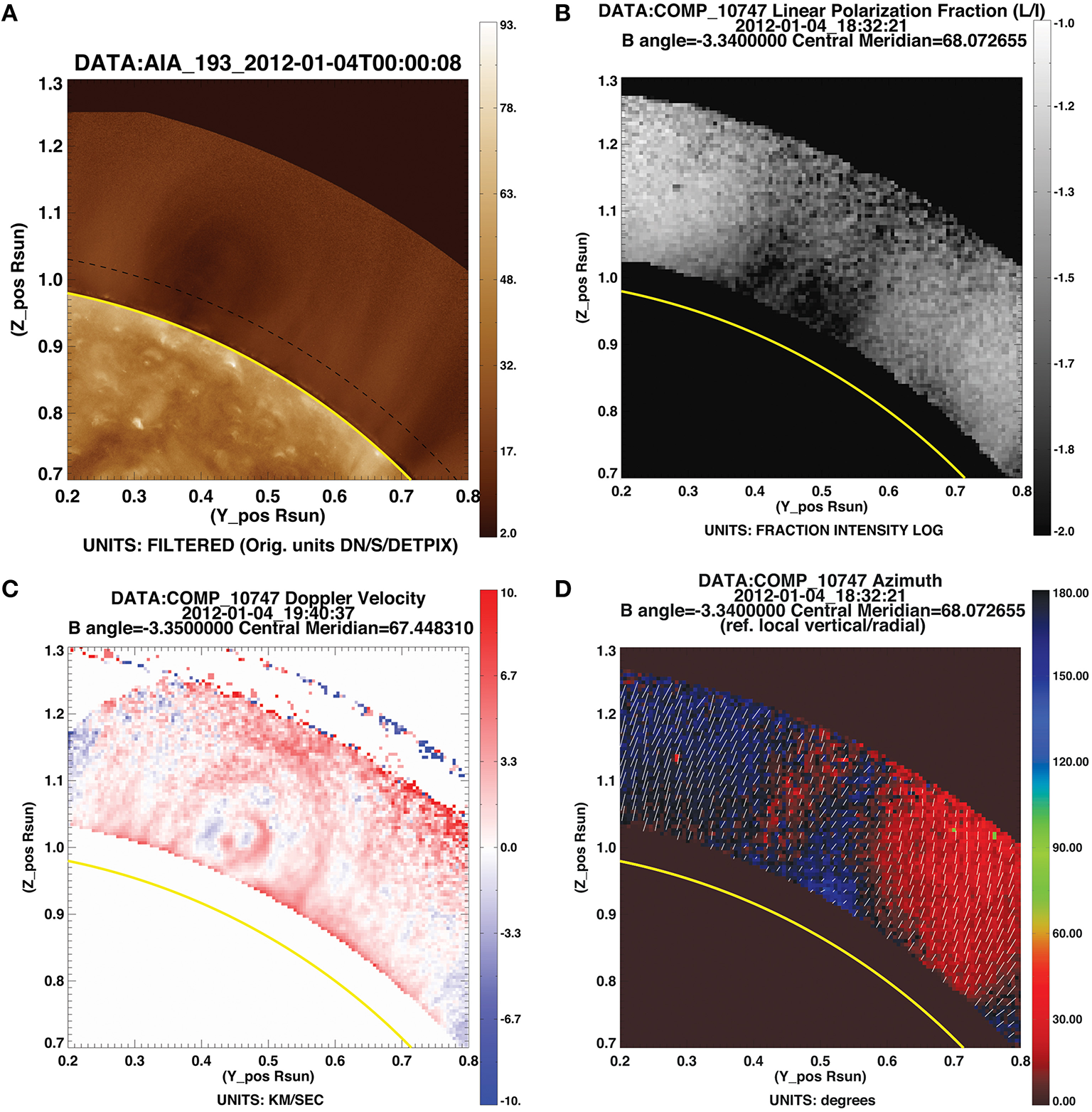
Example of FORWARD-displayed data products for a coronal cavity. (A) SDO/AIA 193 Angstrom. Plot obtained via widget as described in the text, or through IDL line command for_plotfits,date='2012-01-04',/aia,xxmin=.2,xxmax=.8,yymin=.7,yymax=1.3,occult=-1.05, upoccult=1.29. (B) CoMP fraction of linearly-polarized light L/I. Plot obtained via widget and utilizing moreplots option as described in the text, or command as in (A) substituting /comp for /aia, removing occult and upoccult keywords, and adding line='LoI',imin=-2.,imax=-1. (C) CoMP Doppler velocity (partially corrected for solar rotation Tian et al., 2013). Plot displays data from CoMP Dynamics fits file downloaded from MLSO web page (http://www2.hao.ucar.edu/mlso), through widget “By File” option or command as in (A) substituting /comp, removing date and occult, upoccult keywords, and adding filename='20120104.194037.comp.1074.dynamics.3.fts',line='DOPPLERVLOS'. (D) CoMP linear polarization azimuth. Plot obtained by widget or command line as in (A), but substituting /comp, and adding line='Az'.
A range of extreme ultraviolet (EUV) and soft Xray (SXR) imager data is available through the Virtual Solar Observatory (VSO; Hill et al., 2009) and accessed by FORWARD. These include data from the currently operating Solar Dynamics Observatory Atmospheric Imaging Assembly (SDO/AIA) and Hinode X-ray Telescope (XRT), along with prior data from the Solar and Heliospheric Observatory Extreme ultraviolet Imaging Telescope (SOHO/EIT) and Transition Region and Coronal Explorer (TRACE), which provide observations at wavelengths spanning coronal and transition region temperatures. Data from the ProbA-2 “Sun Watcher using APS and Image Processing” (SWAP) EUV imager (Halain et al., 2013; Seaton et al., 2013) provide an extended (54 arcminute) field of view (FOV), and the Solar-Terrestrial Relations Observatory Extreme Ultraviolet Imagers (STEREO/EUVIA and EUVIB) provide additional viewing options for EUV coronal structures.
It is particularly simple to intercompare observations using the widget interface. For example, AIA data may be loaded by date as in Figure 9, and then a particular structure such as the cavity shown in Figure 10A may be zoomed in on using the field of view (FOV-POS) tab of the right-hand widget. By switching on the keyword moreplots (located in the Output tab of the top-left widget), the zoomed-in FOV is retained and closest date/time sought in subsequent loading of CoMP data (b-d). This capability extends to forward-modeled synthetic data: if the moreplots option is turned on and followed by choice of a model and a click on the FORWARD button (top left widget), the field of view, viewer's position, and observable (instrument and line) are all preserved in subsequent forward calculations unless explicitly changed. In this manner, as demonstrated by Figures 11, 12 and discussed in the next section, model predictions may be directly compared to observations.
Figure 11
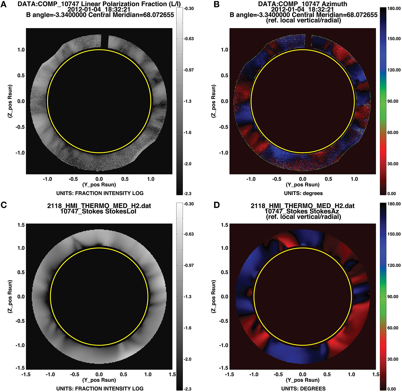
Linear polarization: observations vs. model. (A,B) Fraction and direction of linear polarization. Plots obtained from widget or IDL line commands as in Figures 10B,D, but without the xxmin, xxmax keywords set. (C,D) Same from forward calculation of MAS model. Plots obtained as in Figures 6E,G, with addition of keywords occult=1.05,upoccult=1.29. Alternatively, (C,D) may be obtained by loading (A,B) from the widget, choosing the PSIMAS model from the drop-down menu, and clicking FORWARD.
Figure 12
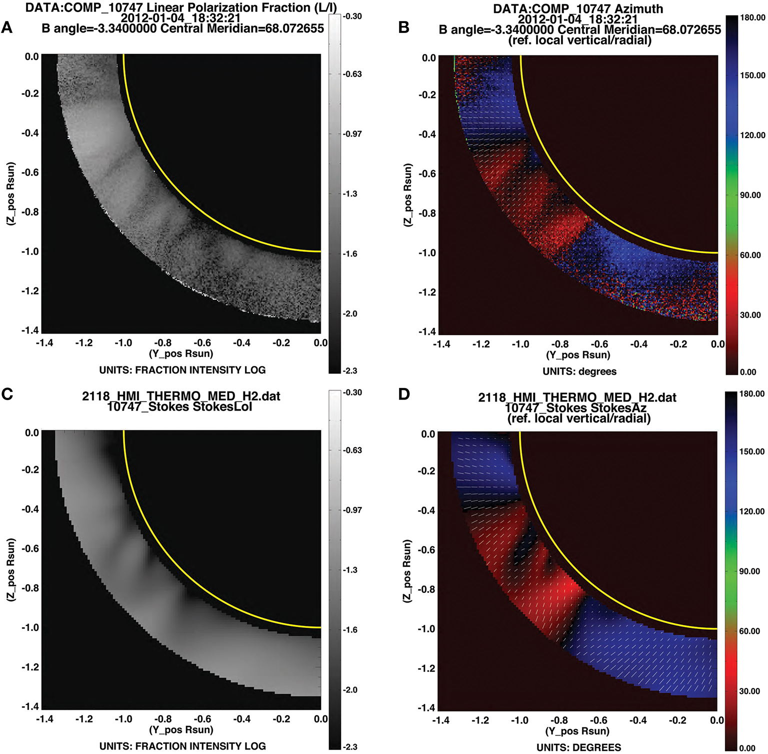
Linear polarization: observations vs. model (A–D) as in Figure 11, but zoomed in to southeast quadrant (keywords set: xxmax=0.,yymax=0).
5. Multiwavelength magnetometry
Having described how FORWARD incorporates the three essential components of physical state, physical process, and observation, we now discuss how it may be used to further multiwavelength magnetometry. FORWARD can be applied to validating models, to building intuition into how magnetic fields manifest in observations, to forward-fitting models to data, and ultimately, to developing coronal magnetic inversion methods that take full advantage of multiwavelength observations.
5.1. Comparing models and data
Figure 11 shows the CoMP observations for the day profiled in most of the Figures so far, allowing validation of the predictions of the MAS model. Inspection shows that while some regions match very well, others do not. For example, Figure 12 illustrates that for the southeast quadrant, the open region of diverging field (just below the equator) is well-captured by the model. Some of the details south of this are not captured, but the red-black-blue interface characteristic of a large-scale closed structure is reproduced. In contrast, the northwest quadrant shows considerably more structure in linear polarization observations (Figure 11A) than in the model (Figure 11C). Figure 10 further magnifies the data in this region, and demonstrates that the northern-most of these linear polarization structures is associated with a coronal cavity. The difference between model and data in this region likely arises because, although the MAS simulation we have shown is non-potential, it does not capture all coronal currents. In particular, currents that slowly build up over time are not reproduced. Such a buildup of currents is expected in polar crown regions (Yeates and Mackay, 2012), and is thus likely in the region of the cavity of Figure 10.
The linear polarization observations of the CoMP telescope represent a unique observational resource, and one that has benefited greatly from the intuition built via forward modeling. In advance of CoMP's synoptic operation at MLSO, the CLE code was used to demonstrate that the presence of currents in the corona should be observable in Fe XIII linear polarization (Judge et al., 2006). Indeed, this has proved the case, and comparisons of CoMP data to FORWARD-generated images have shown linear polarization to be a useful diagnostic of magnetic topologies, including spheromaks (Dove et al., 2011), pseudostreamers (Rachmeler et al., 2014), and cylindrical flux ropes (Ba̧k-Stȩślicka et al., 2013; Rachmeler et al., 2013). The CoMP linear polarization structure shown in Figure 10B is an example of a “lagomorph” (named for its rabbit's-head shape). Ba̧k-Stȩślicka et al. (2013, 2014) studied dozens of examples of CoMP lagomorphs, and showed clear correlation with the size and location of associated EUV prominence cavities (e.g., Figure 10A vs. Figure 10B). The authors also used forward modeling to demonstrate that a magnetic flux rope model results in a lagomorph: the van Vleck angles within the outer portions of the flux rope and the overlying arcade creates a dark structure framing the rabbit's ears and the sides of its head, and sheared or twisted fields at the flux rope's axis, being oriented perpendicular to the plane of sky, are also relatively dark in linear polarization and form the center of the head.
The presence of a wide V shape is expected even for a potential field arcade. Using an analytic model of a flux rope included in FORWARD (Low and Hundhausen, 1995), Figure 13 shows how the addition of coronal currents above the magnetic neutral line narrows this V and introduces a dark central structure. The bottom row of Figure 13 may be compared to Figure 10, noting that the top of the cavity/flux rope is near the top of the CoMP field of view, so that the ears are not captured in this case.
Figure 13
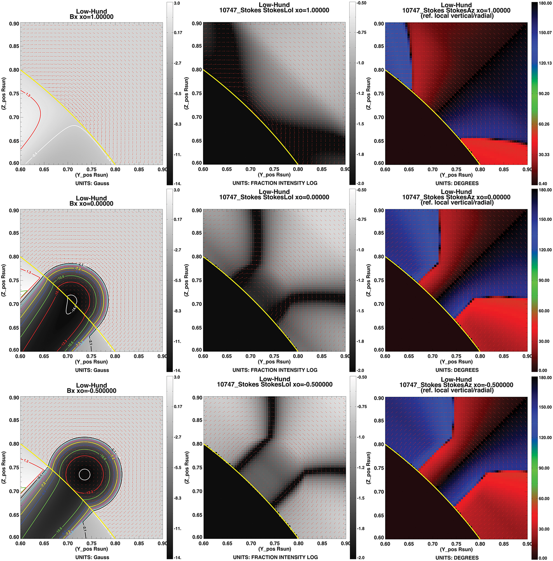
Using an analytic flux-rope model (Low and Hundhausen, 1995), we see that the presence of currents above the underlying neutral line narrows the ears and introduces the dark central head structure to a linear polarization lagomorph. Left column: LOS-oriented magnetic field strength. Plots obtained through commands for_drive, 'lowhund', line='bx', thetao=45.,x_oinput=xo,xxmin=0.6,xxmax=0.9,yymin=0.6,yymax=0.9, /fieldlines,imin=-14,imax=3 for values of xo = 1.,0.,-.5. Middle column: LOS-integrated linear polarization fraction. Plots obtained from same commands, substituting line='LoI',imax=-.5,imin=-2. and adding keyword /comp. Right column: LOS-integrated linear polarization direction (azimuth). Plots obtained as for L/I, but substituting line='Az'.
As we have discussed above, there are a range of multiwavelength observations that can be used to constrain coronal magnetic fields. Indeed, coronal-cavity white light and emission observations have been interpreted as largely independent indicators of a flux-rope magnetic structure (see discussion in Gibson, 2014, 2015a; see also Ba̧k-Stȩślicka et al., in preparation for discussion of LOS flows as indications of magnetic-flux-rope topology). Quantification of the three-dimensional morphology, substructure, and plasma properties of cavities have served to justify such interpretations. These quantifications were obtained by fitting the “CAVMORPH” analytic model included within the FORWARD distribution to observations of cavities in white light, EUV, and SXR (Gibson et al., 2010; Schmit and Gibson, 2011; Kucera et al., 2012; Reeves et al., 2012).
Such “forward fitting” goes beyond intuition building, and in fact is a means of inverting observations to quantify properties of the physical state. It does require specification of a parameterized model, such that through iteration best-fit parameters are determined. Dalmasse et al. (in preparation) provides an example of a statistical method applied to forward fitting a flux-rope model to visible/IR polarimetric data, including both linear and circular polarization (see also Jibben et al., submitted). Other inversion methods applicable to these data are also under development (Kramar et al., 2006, 2013, 2014; Plowman, 2014; also Kramar et al., in preparation).
5.2. Synthetic testbeds and beyond
The method described in Dalmasse et al. (in preparation) employs synthetic Fe XIII linear polarization data generated using FORWARD. This work represents an area of active development for FORWARD, i.e., the creation of multiwavelength synthetic data for coronal magnetic structures ranging from active regions (e.g., M. Rempel, private communication), to polar crown prominence/cavity systems (e.g., Fan, personal communication; see Figure 14, to a global corona containing a variety of currents, e.g., D. Mackay, private communication). These numerical simulations will be included in future FORWARD SolarSoft distributions, and from them synthetic data ranging from radio to SXR wavelengths can be generated as community testbeds to aid in the development of inversion methods and in analyses of the sensitivity of different types of observations to physical parameters.
Figure 14
Synthetic data including (A) visible and (B) EUV intensity, and (C) IR and (D) radio circular polarization, generated for simulated prominence-cavity system (Fan, personal communication). Plot (A) obtained by FORWARD line command: for_drive, 'numcube', cubename='$FORWARD_ DB/TESTBEDS/fullthermodynamic_erupting_qp_mhd_ Fan', xxmin=0.8,xxmax=1.4,yymin=-.5,yymax=.5,units= 'PPM', cuberot=-25.,colortable=0. Plot (B) obtained with addition of keyword /aia. Plot (C) added with addition of keyword /comp,line='VOI', and (D) with addition of /radio,line='VOI'.
The images shown in Figures 1–14 are idealized. Real data has noise, and inversions must take this into account. Sensitivity, field of view and spatial resolution of the telescope used to obtain the data may all contribute to noise. For polarimetry, sensitivity is usually a constraining factor because (at least at optical, IR and UV wavelengths) the polarized signals are much weaker than the total intensities and subject to cross-talk that requires careful time-consuming calibration to ensure robust measurements. With modern telescopes one is also often trading large fields of view for high spatial resolution, and for the observation of spatially extended features this can be a problem.
At radio wavelengths, one has to deal with the fact that spatial resolution is always frequency dependent: for a fixed effective aperture dimension, the size of a resolution element is inversely proportional to frequency, and for typical modern radio observations taken over a wide frequency range, the spatial resolution can vary by factors of several from high to low frequencies. For the purpose of measuring coronal magnetic fields with gyroresonance emission where field strength is proportional to frequency, this means that one generally has poorer spatial resolution for the study of weak fields than for strong fields. Fortunately this is in the right direction since strong-field regions are usually smaller, but it does limit our ability to study three-dimensional fields with uniform resolution.
At the moment, FORWARD only implements noise for visible/IR spectropolarimetry (Section 3.4), and then only photon noise (see Figure 15). Efforts are underway to allow “instrument personality profiles” in which a loss of resolution appropriate to a particular observation could be overlaid on the forward calculation, given details of a telescope and its observing configuration. This capability would enable the design and use of future large telescopes such as the Daniel K. Inouye Solar Telescope (DKIST), the Frequency Agile Solar Telescope (FASR), and the Coronal Solar Magnetism Observatory (COSMO; e.g., Figure 15; see also Lin, 2016).
Figure 15
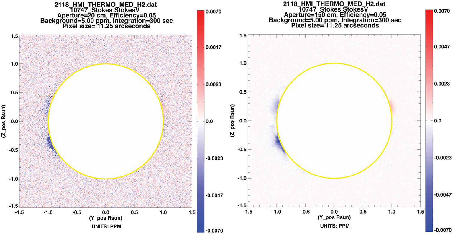
Stokes V/I for MAS model as in Figure 6C, with the addition of photon noise expected for 5 min integration for a 20 cm (e.g., MLSO/CoMP) vs. a 150 cm (e.g., proposed COSMO) telescope. Note systematic errors are not included. Plots obtained by (left) for_drive,readmap='psimas_10747_ 01042012',line= 'V', /donoise and (right) same, with addition of aperture=150.
6. Conclusions
Our primary motivation in developing FORWARD has been to enable multiwavelength coronal magnetometry. The coronal magnetic field lies at the heart of many of the mysteries of solar physics, including coronal heating, solar wind acceleration, and flare and coronal mass ejection onset and evolution. It holds the key to progress in predictive capability for space-weather events: in particular, the direction of the magnetic field at 1 AU depends crucially on the magnetic field at its coronal source, and on the context of this source in both time and space. In this paper we have demonstrated how different physical processes effectively highlight different aspects of the coronal magnetic field, and how these manifest in observations at different wavelengths. Because the photospheric magnetic field is not force-free, our ability to find a meaningful solution to coronal magnetic field through extrapolations from this boundary is limited (De Rosa et al., 2009). We therefore must make use of multiwavelength observations of the solar atmosphere to further constrain the global coronal magnetic field.
FORWARD represents a community effort to design and gather a library of codes for the synthesis of multiwavelength coronal data from physical models. Our philosophy has been to incorporate as many existing resources as possible, and to make use of the comprehensive and ever-growing resources available via SolarSoft IDL. We note complementary capabilities available for forward modeling in radio wavelengths, i.e., the GX_Simulator package referred to above in Section 3.6 (Nita et al., 2015), and for forward modeling coronal waves, i.e., the FoMo codes described in van Doorsselaere et al. (2016).
FORWARD continues to be developed. New subroutines for ultraviolet spectropolarimetry in the unsaturated Hanle regime are being tested (Fineschi, 2001; see also Raouafi et al., submitted; Dima et al., submitted). We are also expanding our numerical interface to allow varied-grid models (currently numerical datacubes must be on a regular grid). A future goal will be to add capability for synthesizing heliospheric images, which would complement current capability for Faraday rotation, and enable connections between imaging and in situ observations during the era of Solar Probe and Solar Orbiter. The wide variety of multiwavelength data currently and soon to be available, in combination with ongoing efforts to develop comprehensive and efficient inversion methods, makes us confident that ultimately the goal of quantifying the coronal magnetic field will be achieved.
Funding
NCAR is supported by the National Science Foundation. SG acknowledges support from the Air Force Office of Space Research, FA9550-15-1-0030. TK acknowledges support from NASA. LR acknowledges support from the Belgian Federal Science Policy Office (BELSPO) through the ESA-PRODEX program, grant No. 4000103240. KR acknowledges support from contract NNM07AB07C from NASA to SAO.
Acknowledgments
We thank Phil Judge and Roberto Casini for their assistance with the utilization and interpretation of the FORTRAN CLE code incorporated within FORWARD, and Roberto Casini for his internal review of this paper. We thank the International Space Science Institute (ISSI) teams on coronal cavities (2008–2010) and coronal magnetism (2013–2014) who were key to initiating and guiding FORWARD development efforts. In particular, we thank Tim Bastian for contributions to the radio codes within FORWARD, and Jeff Kuhn for interesting discussions pertaining to instrument personality profiles (currently under development). We acknowledge Matthias Rempel and Duncan Mackay for contributions of synthetic test-beds for FORWARD. We also acknowledge the Data-Optimized Coronal Field Model (DOC-FM) team and especially Kevin Dalmasse, Silvano Fineschi, Natasha Flyer, Nathaniel Mathews, and Doug Nychka for current engagement in FORWARD development, and Haosheng Lin, Don Schmit, and Chris Bethge for past code contributions. In addition, we acknowledge Enrico Landi for assistance with CHIANTI interfacing, Dominic Zarro for assistance with VSO interfacing, and Sam Freeland for assistance with SolarSoft interfacing. FORWARD makes use of a range of SolarSoft codes developed by others—we are grateful to Marc de Rosa for his PFSS SolarSoft codes, and Andrew Hayes for his routines for the F corona. We acknowledge Leonard Sitongia for initial help with MLSO data access, and Joan Burkepile, Giuliana de Toma, and Steve Tomczyk for ongoing assistance. MLSO is operated by the High Altitude Observatory, as part of the National Center for Atmospheric Research (NCAR). AIA data are courtesy of NASA/SDO and the AIA, EVE, and HMI science teams.
Conflict of interest statement
The authors declare that the research was conducted in the absence of any commercial or financial relationships that could be construed as a potential conflict of interest.
Statements
Author contributions
SG was primary author of this paper, wrote or contributed to most of the subroutines in FORWARD, and is responsible for the oversight of its ongoing development. TK wrote Sections 3.2, 3.3, and contributed to Sections 5, 6. She wrote or otherwise coordinated all FORWARD codes and databases related to EUV/SXR imaging and spectroscopy, and contributed to several other FORWARD subroutines. SW wrote Sections 3.6, 3.7, and contributed to Section 5, 6. He wrote or otherwise coordinated all FORWARD codes related to radio spectropolarimetry. JD was the main author of the integration of CLE into FORWARD, and the initial developer of several of the backbone subroutines of FORWARD as well as the analytic model interface. LR developed the numerical interface and incorporated the PFSS model into FORWARD, and contributed to the data-download interface codes and other FORWARD subroutines. YF contributed to the numerical interface effort, provided an axisymmetric flux rope model to the FORWARD package for demonstration purposes, and is providing numerical simulations for synthetic test-beds as discussed in Section 5. BF was the initial developer of the for_widget interface. CD contributed a subroutine for interfacing with the PSI MAS model and assisted with its implementation. KR contributed the XRT response subroutine. All authors read and critically revised the paper, approved the final version, and agreed to be accountable for all aspects of the work.
Conflict of interest
The authors declare that the research was conducted in the absence of any commercial or financial relationships that could be construed as a potential conflict of interest.
References
1
Ba̧k-StȩślickaU.GibsonS. E.FanY.BethgeC.ForlandB.RachmelerL. A. (2013). The magnetic structure of solar prominence cavities: new observational signature revealed by coronal magnetometry. Astrophys. J.770:28. 10.1088/2041-8205/770/2/L28
2
Ba̧k-StȩślickaU.GibsonS. E.FanY.BethgeC.ForlandB.RachmelerL. A. (2014). The spatial relation between EUV cavities and linear polarization signatures. Proc. Int. Astronom. Union300, 395–396. 10.1017/S1743921313011253
3
BillingsD. E. (1966). A Guide to the Solar Corona. New York, NY: Academic Press.
4
BirdM. K.SchrueferE.VollandH.SieberW. (1980). Coronal faraday rotation during solar occultation of PSR0525 + 21. Nature283, 459. 10.1038/283459a0
5
BirdM. K.VollandH.HowardR. A.KoomenM. J.MichelsD. J.SheeleyJr.N.R.et al. (1985). White-light and radio sounding observations of coronal transients. Solar Phys.98, 341–368. 10.1007/BF00152465
6
CaffauE.LudwigH.-G.SteffenM.FreytagB.BonifacioP. (2011). Solar chemical abundances determined with a CO5BOLD 3D model atmosphere. Solar Phys.268, 255–269. 10.1007/s11207-010-9541-4
7
CasiniR.JudgeP. G. (1999). Spectral Lines for Polarization Measurements of the Coronal Magnetic Field. II. Consistent Treatment of the Stokes Vector forMagnetic-Dipole Transitions. Astrophys. J.522, 524. 10.1086/307629
8
De RosaM. L.SchrijverC. J.BarnesG.LekaK. D.LitesB. W.AschwandenM. J.et al. (2009). A critical assessment of nonlinear force-free field modeling of the solar corona for active region 10953. Astrophys. J.696, 1780–1791. 10.1088/0004-637X/696/2/1780
9
Del ZannaG.DereK. P.YoungP. R.LandiE.MasonH. E. (2015). CHIANTI - An atomic database for emission lines. Version 8. Astron. Astrophys.582:A56. 10.1051/0004-6361/201526827
10
DereK. P.LandiE.MasonH. E.Monsignori FossiB. C.YoungP. R. (1997). CHIANTI - an atomic database for emission lines. Astron. Astrophys. Suppl.125, 149–173. 10.1051/aas:1997368
11
DereK. P.LandiE.YoungP. R.Del ZannaG.LandiniM.MasonH. E. (2009). CHIANTI - an atomic database for emission lines. IX. Ionization rates, recombination rates, ionization equilibria for the elements hydrogen through zinc and updated atomic data. Astron. Astrophys.498, 915–929. 10.1051/0004-6361/200911712
12
DoveJ.GibsonS.RachmelerL. A.TomczykS.JudgeP. (2011). A ring of polarized light: evidence for twisted coronal magnetism in cavities. Astrophys. J. Lett.731:1. 10.1088/2041-8205/731/1/L1
13
DulkG. A. (1985). Radio emission from the sun and stars. Ann. Rev. Astron. Astrophys.23:169. 10.1146/annurev.aa.23.090185.001125
14
FeldmanU.MandelbaumP.SeelyJ. F.DoschekG. A.GurskyH. (1992). The potential for plasma diagnostics from stellar extreme-ultraviolet observations. Astrophys. J. Supp.81, 387–408. 10.1086/191698
15
FineschiS. (2001). Space-based instrumentation for magnetic field studies of solar and stellar atmospheres, in Magnetic Fields Across the Hertzsprung-Russell Diagram, ASP Conference Proceedings, Vol. 248, eds MathysG.SolankiS. K.WickramasingheD. T. (San Francisco, CA: Astronomical Society of the Pacific), 597.
16
ForlandB. F.GibsonS. E.DoveJ. B.KuceraT. A. (2014). The solar physics forward codes: now with widgets. Proc. Int. Astronom. Union300, 414–415. 10.1017/S1743921313011332
17
FreelandS. L.HandyB. N. (1998). Data analysis with the solarSoft system. Solar Phys.182, 497–500. 10.1023/A:1005038224881
18
GelfreikhG. B. (2004). Coronal magnetic field measurements through bremsstrahlung emission, in Solar and Space Weather Radiophysics, eds GaryD. E.KellerC. U. (Dordrecht. Kluwer Academic Publishers), 115–133. 10.1007/1-4020-2814-8_6
19
GibsonS. E. (2014). Magnetism and the invisible man: the mysteries of coronal cavities, in IAU Symposium, Volume 300 of IAU Symposium, eds SchmiederB.MalherbeJ.-M.WuS. T., 139–146.
20
GibsonS. (2015a). Coronal cavities: observations and implications for the magnetic environment of prominences, in Astrophysics and Space Science Library, Vol. 415 of Astrophysics and Space Science Library, eds VialJ.-C.EngvoldO. (Springer), 323–353. 10.1007/978-3-319-10416-4_13
21
GibsonS. (2015b). Data-model comparison using FORWARD and CoMP. Proc. Int. Astronom. Union305, 245–250. 10.1017/S1743921315004846
22
GibsonS. E.FanY. (2006). Coronal prominence structure and dynamics: a magnetic flux rope interpretation. J. Geophys. Res.111:A12103. 10.1029/2006ja011871
23
GibsonS. E.KuceraT. A.RastawickiD.DoveJ.de TomaG.HaoJ.et al. (2010). Three-dimensional morphology of a coronal prominence cavity. Astrophys. J.723:1133. 10.1088/0004-637X/724/2/1133
24
GibsonS. E.LowB. C. (1998). A time-dependent three-dimensional magnetohydrodynamic model of the coronal mass ejection. Astrophys. J.493, 460. 10.1086/305107
25
GrebinskijA.BogodV.GelfreikhG.UrpoS.PohjolainenS.ShibasakiK. (2000). Microwave tomography of solar magnetic fields. Astron. Astrophys. Supp144:169. 10.1051/aas:2000202
26
HabbalS. R.MorganH.DruckmüllerM. (2011). A new view of coronal structures: implications for the source and acceleration of the solar wind, in Astronomical Society of India Conference Series, Vol. 2 of Astronomical Society of India Conference Series, eds ChoudhuriA. R.BanerjeeD.259–269.
27
HalainJ.-P.BerghmansD.SeatonD. B.NiculaB.De GroofA.MierlaM.et al. (2013). The SWAP EUV imaging telescope. Part II: in-flight performance and calibration. solphys286, 67–91. 10.1007/s11207-012-0183-6
28
HillF.MartensP.YoshimuraK.GurmanJ.HourcléJ.DimitoglouG.et al. (2009). The virtual solar observatory - a resource for international heliophysics research. Earth Moon Plan.104, 315–330. 10.1007/s11038-008-9274-7
29
JensenE. A.BirdM. K.AsmarS. W.IessL.AndersonJ. D.RussellC. T. (2005). The cassini solar faraday rotation experiment. Adv. Space Res.36, 1587–1594. 10.1016/j.asr.2005.09.039
30
JensenE. A.BisiM. M.BreenA. R.HeilesC.MinterT.VilasF. (2013). Measurements of faraday rotation through the solar corona during the 2009 solar minimum with the MESSENGER spacecraft. Solar Phys.285, 83–95. 10.1007/s11207-012-0213-4
31
JudgeP. G.CasiniR. (2001). A synthesis code for forbidden coronal lines, in Advanced Solar Polarimetry—Theory, Observation, and Instrumentation, 20TH NSO/Sac Summer Workshop, ASP Conference Proceedings, Vol. 236, of Astronomical Society of the Pacific Conference Series (San Francisco, CA: Astronomical Society of the Pacific), 503.
32
JudgeP. G.LowB. C.CasiniR. (2006). Spectral lines for polarization measurements of the coronal magnetic field. iv. stokes signals in current-carrying fields. Astrophys. J.651:1229. 10.1086/507982
33
KarpenJ. (2014). Plasma structure and dynamics, in Solar Prominences, Vol. 415, of Astrophysics and Space Science Library, eds EngvoldO.VialJ. C. (Springer), 237–257. 10.1007/978-3-319-10416-4_10
34
KeadyJ. J.KilcreaseD. P. (2000). Radiation, in Allens Astrophysical Quantities, ed CoxA. N. (New York, NY: AIP), 95–120.
35
KooiJ. E.FischerP. D.BuffoJ. J.SpanglerS. R. (2014). Measurements of coronal faraday rotation at 4.6 R⊙. Astrophys. J.784:68. 10.1088/0004-637X/784/1/68
36
KoppR. A.HolzerT. E. (1976). Dynamics of coronal hole regions. I - Steady polytropic flows with multiple critical points. Solar Phys.49, 43–56.
37
KoutchmyS.LamyP. L. (1985). The F-corona and the circum-solar dust evidences and properties, in IAU Colloq. 85: Properties and Interactions of Interplanetary Dust, Vol. 119 of Astrophysics and Space Science Library, eds GieseR. H.LamyP. (Springer), 63–74.
38
KramarM.AirapetianV.MikićZ.DavilaJ. (2014). 3D coronal density reconstruction and retrieving the magnetic field structure during solar minimum. Solar Phys.289, 2927–2944. 10.1007/s11207-014-0525-7
39
KramarM.InhesterB.LinH.DavilaJ. (2013). Vector tomography for the coronal magnetic field. II. Hanle effect measurements. Astron. Astrophys.775, 25. 10.1088/0004-637x/775/1/25
40
KramarM.InhesterB.SolankiS. K. (2006). Vector tomography for the coronal magnetic field. I. Longitudinal Zeeman effect measurements. Astron. Astrophys.456, 665–673. 10.1051/0004-6361:20064865
41
KuceraT. (2015). Solar Prominences, Astrophysics and Space Science Library, Vol. 415, eds EngvoldO.VialJ. C. (Switzerland: Springer International Publishing Switzerland), 79. 10.1007/978-3-319-10416-4_4
42
KuceraT. A.GibsonS. E.SchmitD. J.LandiE.TripathiD. (2012). Temperature and euv intensity in a coronal prominence cavity. Astrophys. J.757:73. 10.1088/0004-637X/757/1/73
43
KunduM. R. (1965). Solar Radio Astronomy. New York, NY: Interscience Publishers.
44
LinH. (2016). mxCSM: A 100-slit, 6-wavelength wide-field coronal spectropolarimeter for the study of the dynamics and the magnetic fields of the solar corona. Front. Astron. Space Sci.3:9. 10.3389/fspas.2016.00009
45
LionelloR.LinkerJ. A.MikicZ. (2009). Multispectral emission of the sun during the first whole sun month. Astrophys. J.690:902. 10.1088/0004-637X/690/1/902
46
LionelloR.WinebargerA. R.MokY.LinkerJ. A.MikićZ. (2013). Thermal non-equilibrium revisited: a heating model for coronal loops. Astrophys. J.773:134. 10.1088/0004-637X/773/2/134
47
LitesB. W.LowB. C. (1997). Flux emergence and prominences: a new scenario for 3-dimensional field geometry based on observations with the advanced stokes polarimeter. Solar Phys.174, 91. 10.1023/A:1004936204808
48
LowB. C.HundhausenJ. R. (1995). Magnetostatic structures of the solar corona. ii. the magnetic topology of quiescent prominences. Astrophys. J.443, 818. 10.1086/175572
49
LunaM.KarpenJ. T.DeVoreC. R. (2012). Formation and evolution of a multi-threaded solar prominence. Astrophys. J.746, 30. 10.1088/0004-637X/746/1/30
50
MalanushenkoA.SchrijverC. J.DeRosaM. L.WheatlandM. S. (2014). Using coronal loops to reconstruct the magnetic field of an active region before and after a major flare. Solar Stell. Astrophys.783, 102. 10.1088/0004-637x/783/2/102
51
MancusoS.SpanglerS. R. (2000). Faraday rotation and models for the plasma structure of the solar corona. Astrophys. J.539, 480–491. 10.1086/309205
52
MannI. (1992). The solar F-corona - calculations of the optical and infrared brightness of circumsolar dust. Solar Phys.261, 329–335.
53
MorganH.HabbalS. R.WooR. (2006). The depiction of coronal structure in white-light images. Astrophysics236, 263–272. 10.1007/s11207-006-0113-6
54
MunroR. H.JacksonB. V. (1977). Physical properties of a polar coronal hole from 2 to 5 solar radii. Astrophys. J.213, 874. 10.1086/155220
55
NewkirkG.AltschulerM. D. (1970). Magnetic fields and the solar corona. III: the observed connection between magnetic fields and the density structure of the corona. Solar Phys.13, 131–152. 10.1007/BF00963948
56
NitaG. M.FleishmanG. D.KuznetsovA. A.KontarE. P.GaryD. E. (2015). Three-dimensional radio and X-ray modeling and data analysis software: revealing flare complexity. Astrophys. J.799, 236. 10.1088/0004-637X/799/2/236
57
OrdS. M.JohnstonS.SarkissianJ. (2007). The magnetic field of the solar corona from pulsar observations. Solar Phys.245, 109–120. 10.1007/s11207-007-9030-6
58
PlowmanJ. (2014). Single-point inversion of the coronal magnetic field. Astrophys. J.792, 23. 10.1088/0004-637X/792/1/23
59
RachmelerL. A.GibsonS. E.DoveJ. B.DeVoreC. R.FanY. (2013). Polarimetric properties of flux ropes and sheared arcades in coronal prominence cavities. Solar. Phys.288, 617–636. 10.1007/s11207-013-0325-5
60
RachmelerL. A.PlattenS. J.BethgeC.SeatonD. B.YeatesA. R. (2014). Observations of a hybrid double-streamer/pseudostreamer in the solar corona. Solar Stell. Astrophys.787, L3. 10.1088/2041-8205/787/1/l3
61
ReevesK. K.GibsonS. E.KuceraT. A.HudsonH. S. (2012). Thermal properties of coronal cavities observed with the X-ray telescope on Hinode. Astrophys. J.746:146. 10.1088/0004-637X/746/2/146
62
RobinsonP. A.MelroseD. B. (1984). Gyromagnetic emission and absorption: approximate formulas of wide validity. Aust. J. Phys.37, 675. 10.1071/PH840675
63
SavchevaA. A.McKillopS. C.McCauleyP. I.HansonE. M.DeLucaE. E. (2013). A new sigmoid catalog from hinode and the solar dynamics observatory: statistical properties and evolutionary histories. Solar Phys.289, 3297–3311. 10.1007/s11207-013-0469-3
64
SchmelzJ. T.ReamesD. V.von SteigerR.BasuS. (2012). Composition of the solar corona, solar wind, and solar energetic particles. Astrophys. J.755, 33. 10.1088/0004-637X/755/1/33
65
SchmidtJ. M.CairnsI. H. (2012a). Type II radio bursts: 1. New entirely analytic formalism for the electron beams, Langmuir waves, and radio emission. J. Geophys. Res.117, 4106. 10.1029/2011ja017318
66
SchmidtJ. M.CairnsI. H. (2012b). Type II radio bursts: 2. Application of the new analytic formalism. J. Geophys. Res.117, 11104. 10.1029/2012JA017932
67
SchmitD. J.GibsonS. E. (2011). Forward modeling cavity density: a multi-instrument diagnostic. Astrophys. J.733:1. 10.1088/0004-637X/733/1/1
68
SeatonD. B.BerghmansD.NiculaB.HalainJ.-P.De GroofA.ThibertT.et al. (2013). The SWAP EUV imaging telescope part I: instrument overview and pre-flight testing. Solar. Phys.286, 43–65. 10.1007/s11207-012-0114-6
69
TianH.TomczykS.McIntoshS. W.BethgeC.de TomaG.GibsonS. (2013). Observations of coronal mass ejections with the coronal multichannel polarimeter. Solar Phys.288, 637–650. 10.1007/s11207-013-0317-5
70
TomczykS.CardG. L.DarnellT.ElmoreD. F.LullR.NelsonP. G.et al. (2008). An instrument to measure coronal emission line polarization. Solar Phys.247:411. 10.1007/s11207-007-9103-6
71
TomczykS.McIntoshS. W.KeilS. L.JudgeP. G. (2007). Alfven waves in the solar corona. Science317:1192. 10.1126/science.1143304
72
van DoorsselaereT.AntolinP.YuanD.ReznikovaV.MagyarN. (2016). Forward modeling of EUV and gyrosynchrotron emission from coronal plasmas with FoMo. Front. Astron. Space Sci.3:4. 10.3389/fspas.2016.00004
73
van VleckJ. H. (1925). On the quantum theory of the polarization of resonance radiation in magnetic fields. Proc. Natl. Acad. Sci. U.S.A.11:612. 10.1073/pnas.11.10.612
74
WhiteS. M. (2000). Radio versus euv/x–ray observations of the solar atmosphere. Solar Phys.190, 309. 10.1023/A:1005253501584
75
WhiteS. M.KunduM. R. (1997). Radio observations of gyroresonance emission from coronal magnetic fields. Solar Phys.174, 31. 10.1023/A:1004975528106
76
WhiteS. M.ThejappaG.KunduM. R. (1992). Mode coupling in the solar corona and bipolar noise storms. Solar Phys.138, 163. 10.1007/BF00146202
77
XiaC.KeppensR.AntolinP.PorthO. (2014). Simulating the in situ condensation process of solar prominences. Solar Stell. Astrophys.792, L38. 10.1088/2041-8205/792/2/l38
78
YeatesA. R.MackayD. H. (2012). Chirality of high-latitude filaments over solar cycle 23. Solar Stell. Astrophys.753, L34. 10.1088/2041-8205/753/2/l34
79
YouX. P.ColesW. A.HobbsG. B.ManchesterR. N. (2012). Measurement of the electron density and magnetic field of the solar wind using millisecond pulsars. Monthly Notices R. Astron. Soc.422, 1160–1165. 10.1111/j.1365-2966.2012.20688.x
Summary
Keywords
sun: corona, sun: magnetic fields, sun: x-rays, sun: radio, sun: infrared, sun: EUV
Citation
Gibson SE, Kucera TA, White SM, Dove JB, Fan Y, Forland BC, Rachmeler LA, Downs C and Reeves KK (2016) FORWARD: A Toolset for Multiwavelength Coronal Magnetometry. Front. Astron. Space Sci. 3:8. doi: 10.3389/fspas.2016.00008
Received
06 January 2016
Accepted
24 February 2016
Published
15 March 2016
Volume
3 - 2016
Edited by
Xueshang Feng, National Space Science Center, China
Reviewed by
Satoshi Inoue, Max-Planck Institute for Solar System Research, Germany; Jiansen He, Peking University, China
Updates
Copyright
© 2016 Gibson, Kucera, White, Dove, Fan, Forland, Rachmeler, Downs and Reeves.
This is an open-access article distributed under the terms of the Creative Commons Attribution License (CC BY). The use, distribution or reproduction in other forums is permitted, provided the original author(s) or licensor are credited and that the original publication in this journal is cited, in accordance with accepted academic practice. No use, distribution or reproduction is permitted which does not comply with these terms.
*Correspondence: Sarah E. Gibson sgibson@ucar.edu
This article was submitted to Stellar and Solar Physics, a section of the journal Frontiers in Astronomy and Space Sciences
Disclaimer
All claims expressed in this article are solely those of the authors and do not necessarily represent those of their affiliated organizations, or those of the publisher, the editors and the reviewers. Any product that may be evaluated in this article or claim that may be made by its manufacturer is not guaranteed or endorsed by the publisher.