Evidence for a Magnetic Flux Rope in Observations of a Solar Prominence-Cavity System

1. Introduction

Solar prominences are sheets of cool dense plasma suspended in the solar corona observed on the limb. Their formation and stability require several mechanisms working in tandem. It is widely accepted that the magnetic field provides the structural support of the prominence but direct observations of the magnetic field in the corona are not currently available. Comprehensive reviews of prominence systems and their dynamics are provided by Martin (1990), Mackay et al. (2010), Parenti (2014), Priest (2014), and Vial and Engvold (2015) and we will provide a brief review here. Prominences only form between regions of opposite magnetic field polarity. In other words, along the polarity inversion line (PIL; Smith, 1968; Martin, 1973). But not all PILs will exhibit prominence formation; another condition required is a predominant transverse magnetic field aligned with the long axis of the prominence. The path in the chromosphere where this happens is referred to as a filament channel (Martin, 1990). Along filament channels, there is a significant decrease in the number of observed spicules compared to the surrounding area (Martin, 1990). Reduced spicule activity indicates weak radial magnetic fields and quiescent prominences may form along giant cell boundaries that separate unipolar magnetic field regions (Malherbe and Priest, 1983; Schröter et al., 1987). Bipoles within the filament channel are often characterized by a bald-patch topology (Titov and Démoulin, 1999) where the magnetic field at the photosphere is largely horizontal and points from negative to positive polarity (López Ariste et al., 2006). The long-term converging patches of opposite polarity flow into juxtaposition along the PIL and as they encounter one another, they disappear concurrently at their boundaries (Martin, 1990). Finally, prominences will quickly dissipate unless there is a closed arcade of magnetic field lines overlying and connecting regions of opposite polarity. The closed loops not only hold down the prominence material but they also create a magnetically stable system in which the cool prominence material interacts with the hot plasmas in the corona.

Under the arcade, a region of reduced coronal emission (the coronal cavity) can develop above quiescent prominences (Vaiana et al., 1973). Despite their reduced coronal emissions, these cavities are filled with complex, twisted structures when observed in white light eclipse data and are distinct from the magnetic structures defining the rest of the overlying arcade that forms the base of streamers as well as the boundaries of streamers (Habbal et al., 2010). This suggests the overlying arcade and underlying prominence are independent magnetic structures that can interact via magnetic reconnection at their boundaries. Therefore, the magnetic structure of the cavity and prominence system prior to an eruption is important to understanding how instabilities form.

A magnetic flux rope is often used to model the prominence and cavity system (Priest et al., 1989; Rust and Kumar, 1994; van Ballegooijen, 2004), with much of the prominence material sitting in the dips of the magnetic field lines (Kuperus and Raadu, 1974; Pneuman, 1983; Priest et al., 1989; van Ballegooijen and Martens, 1989; Rust and Kumar, 1994; Low and Hundhausen, 1995; Aulanier et al., 1998; Chae et al., 2001; van Ballegooijen, 2004; Gibson et al., 2006; Dudík et al., 2008). Fan and Gibson (2006) modeled a prominence as a twisted flux rope and found that a current sheet forms within the flux rope cavity along a bald-patch separatrix surface (BPSS), composed of the field lines that graze the anchoring lower boundary, enclosing the detached helical field that supports the prominence. They further show that resistive dissipation of the current sheet would produce a hot sheath surrounding the prominence material in the cavity, which could provide an explanation for the observed development of X-ray bright cores within a coronal cavity (Hudson et al., 1999; Hudson and Schwenn, 2000; Reeves et al., 2012). Su et al. (2015) constructed a series of magnetic field models with different configurations based on the observed photospheric magnetogram for a polar crown prominence, and they found that the model with a twisted flux rope best matches the observations.

Coronal magnetic fields provide the structure and support for the coronal cavity, but measuring coronal magnetic fields is difficult to do (Lin et al., 2004). Fortunately, some information about the coronal magnetic fields making up coronal cavities has been achieved with the Coronal Multi-Channel Polarimeter (Tomczyk et al., 2008; CoMP). A recent statistical study by Ba̧k-Stȩślicka et al. (2013) found that quiescent prominence cavities consistently posses a “lagomorphic” signature in linear polarization indicating twist or shear extending up into the cavity above the PIL. They also compared the CoMP observations with synthetic CoMP-like data created using a forward magnetohydrodynamics (MHD) model and concluded that a cylindrical magnetic flux rope better represents polar-crown prominence cavities.

In this paper, we present chromospheric and coronal observations of a prominence-cavity system observed on the west limb. We develop a magnetic field model of the system based on these observations. We utilize data from Hinode (Kosugi et al., 2007), Interface Region Imaging Spectrograph (IRIS; De Pontieu et al., 2014), and the Solar Dynamics Observatory's Atmospheric Imaging Assembly (AIA; Lemen et al., 2012) and Helioseismic and Magnetic Imager (HMI; Schou et al., 2012). Together, these instruments provide near simultaneous multithermal observations of the prominence-cavity system and its surroundings. The X-Ray Telescope (XRT; Golub et al., 2007) observes some of the hottest coronal temperatures between 2 and 10 MK. The EUV Imaging Spectrometer (EIS; Culhane et al., 2007) takes spectral data from the transition region to coronal temperatures. Finally, the Solar Optical Telescope (SOT; Tsuneta et al., 2008) and IRIS image chromospheric and transition region plasmas. We use photospheric line-of-sight (LOS) magnetic field data to derive a model of the structure of the system with the assumption it is a magnetic flux rope under an arcade. We vary the axial and poloidal fluxes of the model to best fit the observations and then we compare the coronal features predicted by the model with CoMP observations. We find evidence of heating within the cavity during an eruption and we find evidence that magnetic bipoles within the filament channel exhibit a bald-patch topology. Therefore, we conclude that a weakly twisted magnetic flux rope best represents the prominence-cavity system but further instrumentation is needed to resolve coronal magnetic signatures of a quiescent flux rope within the corona.

2. Materials and Methods

The observations we use were part of an IRIS and Hinode Joint Observation Program (IHOP 264¹) that included observations from all three Hinode instruments. The IHOP was run three times pointing at the same prominence on the west limb between 9 and 10 October 2014. We present the data taken between 18 and 22 UT on 9 October because CoMP was also observing at this time. We do not use the other two data sets because they either do not have corresponding CoMP observations or in the case of the 10 October data, a non-related filament erupted.

2.1. Hinode XRT, EIS, and SOT Data Reduction

The XRT observations used in this study include 8 s thin-Be exposures at 60 s cadence. The field of view is ≈ 790″ × 790″ and the images are binned 2 × 2 giving a resolution of 2.″0572 per pixel. Observations were paused during times when Hinode passed through the South Atlantic Anomaly (SAA) causing 20–30 min gaps in the data. The data is processed using standard data reduction routines provided by the XRT team (Kobelski et al., 2014) and aligned using the database developed by Yoshimura and McKenzie (2015) distributed in SolarSoft (Freeland and Handy, 1998). Either individual or 5 min averaged data were spatially enhanced using the àtrous wavelet transform with a cubic spline scaling function. See page 29, and Appendix A in Stark and Murtagh (2002) for a complete description of the routine. This method separates the image into different spatial scales based on pixel size along with a residual image containing the portion of the image outside of the spatial scales. We display the data without the residual image using a log-like scale so that only bright features with intensity gradients that vary over 1–3 pixels remain. Regions that do not change rapidly are threshold to white or are set to be transparent.

The EIS data utilize the 2″ slit with 50 s exposures, 75 raster positions with binning along the x-direction giving a 300″ × 512″ FOV. Two raster scans are used in this study. The two scans were taken between 18:16–19:21 UT and 19:21–20:26 UT. The scans are processed in IDL using software provided by the EIS team and a thorough discussion of the routines is provided in the EIS data analysis guide². A brief overview is given here.

The data are calibrated using EIS_PREP with the default parameters outlined in the analysis guide. We use three coronal lines for this study, Fe XII 195.12 Å, Fe XIII 202.04 Å, and Fe XV 284.16 Å. The Fe XV 284.16 Å spectra is imaged on a different camera resulting in a slightly different field of view. The lines are fit with a Gaussian profile using EIS_AUTO_FIT routine (Young, 2013). From this, intensity, LOS Doppler velocity maps and line width maps are created.

The default velocity scale used in the data reduction software is derived using the Kamio method (Kamio et al., 2010). We update the velocity scale using a patch of quiet sun. We assume that the LOS velocities will average to zero in this region for each of the spectral lines (Warren et al., 2011). The off limb patch contains 120 pixels in the y-direction and we bin the data by 20 pixels at each raster position, a Gaussian profile is fit to the average of the bottom 6 binned pixels, thus defining the reference wavelength. We perform this procedure for each line separately because an absolute velocity scale cannot be derived for the Fe XV 284.16 Å line with respect to the other two since it is on a separate camera. The error in the velocity is provided from the routines used to generate the velocities.

The SOT data consists of ≈112″ × 112″ Ca II H-line images taken at 30 s cadence between 18 and 20 UT and then 60 s cadence from 20 to 22 UT. The data are calibrated using routines provided in SolarSoft. In addition, the images are spatially enhanced using the same method used on the XRT data except the residual image is preserved. Small scale features are enhanced before recombining the image, which acts to sharpen the image while preserving information about the enhancement. After the images are spatially enhanced, a radial density filter is applied to reduce the intensity of the disk and spicule regions. The radial density filter applied is similar to the one described in Berger et al. (2010). After the images are scaled and sharpened they are aligned using the SolarSoft routine fg_rigidalign.pro. There was a shift in the SOT pointing between the 21:07 and 21:08 frames. The images after 21:08 UT are aligned manually by aligning features visible in both images. Features in SOT are compared with features in AIA 211 Å to coalign SOT with other instruments.

2.2. IRIS Data Reduction

IRIS performed a 16-step coarse raster from 18:24 UT to 21:58 UT. The telescope was pointed on the west limb at 803″, −546″ capturing most of the prominence. The raster field of view was 30″ × 119″ with a raster step cadence of 9.4 s making a raster cadence of 150 s with 8 s exposures. Two broadband filter (2796 and 1400 Å) slit-jaw images (SJI) were taken at a cadence of 19 s with a 119″ × 119″ field of view. The calibrated level 2 data were used in this study and downloaded from the IRIS website³. The prominence material is significantly dimmer than on-disk regions for the chosen lines. To simultaneously observe both regions, we apply an intensity filter to the Si IV 1400 Å images decreasing the on-disk and spicule intensities. The on-disk intensity is decreased by 90% of its original intensity. The intensity of the spicule region is linearly increased from 10 to 100% at the edge of the spicule region. The intensity of the prominence and off limb features do not have their intensity altered. The resultant images are displayed using a square-root inverse intensity scaling.

We use the Mg II 2796 Å and Si IV 1394 Å spectra for this study. The Mg II h and k lines are formed at chromospheric temperature (10⁴ K). Emission from the Si IV 1394 Å line form in the prominence transition region (PCTR). The UV continuum at 1400 Å formed in the lower chromosphere is not present for a prominence observed at the limb contrary to observations on the disk (Schmieder et al., 2014).

We perform a relative wavelength calibration to measure the Doppler velocities of the eruption. The reference wavelength for each spectral line window is selected at the centroid of the line profile averaged over the on-disk scan positions for each raster scan. Therefore, the relative Doppler velocities are measured with respect to the quiet Sun regions. The absolute uncertainty of the relative wavelength calibration is estimated to be 4 km s⁻¹ by Liu et al. (2015). Their estimates include a wavelength shift, 20 mÅ from disk center to the limb and the IRIS orbital thermal variation of 3 km s⁻¹. In that paper, portions of the IRIS slit were on the disk throughout the observations.

2.3. CoMP Data Reduction

CoMP makes daily polarimetric (Stokes I, Q, U, V) of the forbidden lines of Fe XIII at 1074.4 nm and 1078.9 nm with a FOV of 1.4–2 R_ʘ. The degree of linear polarization (L/I) constrains the direction of the plane-of-sky (POS) magnetic field. The amount of circular polarization (V/I) provides information about the strength of the magnetic field along the LOS. The CoMP data consists of QuickInvert data of the Fe XIII 1074.7 nm coronal emission line. The data were downloaded from the High Altitude Observatory/Mauna Loa Solar Observatory website⁴. The Quick Invert files contain five images: Stokes I, Q, U, linear polarization (L), and magnetic field azimuth. The file is read into the FORWARD (Gibson et al., 2016) toolset where L/I is calculated and used for this study.

2.4. Magnetic Model of Prominence-Cavity System

A three-dimensional magnetic model of the prominence-cavity system is constructed using the Coronal Modeling System (CMS) developed by van Ballegooijen (2004). The CMS model assumes the prominence material is supported against gravity by a helical flux rope. The model utilizes SDO/HMI magnetograms to establish the magnetic field strength and topology at the photosphere where it is assumed to be radial. The model is constructed by inserting a flux rope along the PIL under a potential field representing the overlying coronal arcade. The axial flux (in Mx) and the poloidal flux per unit length (in Mx/cm) along the filament are set to an initial value and then magnetofrictional relaxation is used to drive the system to a nonlinear force free state. Detailed description of the methodology can be found in the literature and references therein (Su et al., 2009, 2011; Su and van Ballegooijen, 2012) and we describe the method briefly below.

First, the potential field is computed from the observed magnetic maps. Then, by appropriate modifications of the vector potentials a “cavity” is created above the selected path, and a thin flux bundle, representing the axial flux of the flux rope, is inserted into the cavity with the footpoints of the flux rope embedded in regions near the PIL. The footpoints are chosen so that the flux rope begins and ends in a patch of positive and negative polarity, respectively. To preserve the radial component of the inner boundary, the patch representing the footpoints is removed/added from the photospheric flux distribution and is equal to the axial flux of the inserted flux rope. The poloidal flux is inserted by adding circular loops around the flux bundle (Su et al., 2015). The inserted flux rope is not in force-free equilibrium. We use magneto-frictional relaxation to drive the field toward a force-free state. This method is an iterative relaxation method (van Ballegooijen et al., 2000) specifically designed for use with vector potentials. Magnetofriction has the effect of expanding the flux rope until its magnetic pressure balances the magnetic tension applied by the surrounding potential arcade. Significant magnetic reconnection between the inserted flux rope and the ambient flux may occur during the relaxation process. Therefore, the end points of the flux rope in the relaxed model may be different from that in the original model (Su et al., 2015).

The region around the filament is modeled with high spatial resolution (HIRES) on a variable grid, while more distant regions have a lower resolution on a uniform grid. The HIRES region may contain electric currents, whereas the global model is a current-free potential field. The lower boundary condition for the HIRES region is derived by combining several LOS photospheric magnetograms obtained with the SDO/HMI as these provide better signal to noise than vector magnetograms in quiet sun regions. Since the prominence is observed near the west limb, we use magnetograms that are taken several days before the prominence reaches the limb. We combine four magnetograms, each taken at 19:00 UT, between 2014 October 2–5 to construct a high-resolution map of the radial component B_r of the magnetic field as a function of longitude and latitude at the lower boundary of the HIRES region (0.002 R_ʘ) (Su et al., 2015). The high-resolution computational domain extends about 117° in longitude, 36° in latitude, and up to 2.05 R_ʘ from the Sun. We use the corresponding HMI synoptic map of B_r to compute a low-resolution (1°) global potential field, which provides the side boundary conditions for the HIRES domain, and allows us to trace field lines that pass through the side boundaries of the HIRES region (Su et al., 2015).

We construct a series of models with different combinations of axial and poloidal fluxes of the inserted flux rope. We compare each model with the size, location, and shape of the filament channel and cavity, including the emission structure on the two sides of the filament channel as well as the trajectory of plasma motions. We require the best-fit model to have an overall structure consistent with the observed LOS velocities observed by IRIS and EIS.

2.4.1. Forward Modeling of Stokes Profiles

To compare the models with the CoMP we calculate what the expected L/I would be for our models. To calculate the Stokes vector produced along a given LOS for the magnetic field models, we use the forward models developed by Judge and Casini (2001) and implemented in the FORWARD (Gibson et al., 2016) suite of IDL codes. The FORWARD database is available to the public⁵ and details are provided at the website and in the literature including Rachmeler et al. (2013). A brief summary is provided here.

The forward code uses the magnetic field, temperature, density, and velocity along the LOS to calculate the level population and emitted polarization profile for the Fe XIII 1074.7 nm transition. For our model, we assume an exponential isothermal atmosphere with a temperature of 1.5 MK and use HYDROCALC.pro to calculate the remaining parameters required for the forward calculations. It outputs Stokes I, Q, U, V and for the purpose of this study we use the relative linear polarization (L/I) and relative circular polarization (V/I). The models were based on SDO/HMI magnetograms and were initially rotated to the 2014-10-04 23:59 UT. To compare with the CoMP observations, the models were rotated to the limb so that they match the observation time of the CoMP QuickInvert data, at 21:13 UT.

3. Results

3.1. Observations

The prominence is composed of two linear structures with a N-S oriented component and an E-W component with a southern pitch. Figure 1 shows what the prominence looked like in AIA 193 Å on 4 October 2014 at 18:18 UT (left) and at the beginning of the observation campaign at 18:24 UT on October 9 (right). It is sandwiched between several active regions to the north and the polar coronal hole to the south. The Sun is active during this period with small scale flares and coronal mass ejections associated with the active regions and numerous filaments on the disk.

FIGURE 1

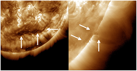
Figure 1. AIA 193 Å observations of the filament. Left: 4 October 2014 at 18:18:06 UT. Right: 9 October 2014 at 18:24:42 UT. The arrows point to the prominence location.

The X-ray data displayed in Figure 2 shows a small coronal cavity associated with the prominence. Figures 2A,B demonstrate how the region (inside black box) looked near the beginning of the observation run. There are several bright formations and it is not apparent which structures, if any, are associated with the prominence. The region remains stable until at 19:09 UT when there is an increase in X-ray emission just above the limb. The black arrows in Figures 2C,D point to this region of increased X-ray emission in the 19:15 UT image. This is the last image XRT took until 19:42 UT, Figures 2E,F. At this time, the X-ray emission has increased around a circular structure which we identify as the cavity. Furthermore, there is now X-ray emission near the center of the cavity that persists throughout the remainder of the observations. Figures 2G,H shows the cavity near the end of the observation run. Black arrows point to the bright X-ray emission near the center of the cavity.

FIGURE 2

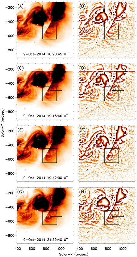
Figure 2. Left column: Hinode XRT thin-Be (inverse log) intensity (5 min average) observations of the coronal cavity. Right column: Spatially enhanced image with the background emission threshold to white. Panels (A,B) shows the cavity prior to the eruption. Panels (C,D) shows the initial phase of the eruption with an arrow pointing to an increase in X-ray emission. Panels (E–H) show the cavity during and after the eruption with the arrows pointing to an increase in X-ray emission within the cavity.

The coronal cavity and overlying arcade are also well sampled with EIS. Figures 3, 4 compare raster scans before and during the eruption. The top row of Figure 3 relates the intensity map (inverse log) for the three Fe lines of the prominence system prior to the eruption. The vertical white stripes represent missing data. The outline of the prominence as seen in Fe XV is overlaid for each image. The southern edge of the cavity is seen in the Fe XII 195.12 Å and Fe XIII 202.04 Å lines as a sharp decrease in intensity just south of the prominence starting from the limb at (770″, −570″) extending radially out to the edge of the field of view. Interestingly, the Fe XV 284.16 Å line does not show this trend. The Doppler velocity map (middle row) shows a quiet region lacking large-scale LOS flows. Velocities that fall within the error for the measurements are scaled to white. The images showing line widths (bottom row) exhibit some regions around the prominence with higher than average widths, especially in the Fe XV 284.16 Å line. These elevated line widths could indicate that turbulent motions are present.

FIGURE 3

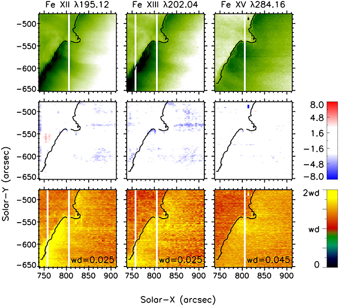
Figure 3. A subfield of the EIS raster scan starting from the left at 18:16 UT and finishing at 19:21 UT. Top row: EIS intensity (inverse log) for Fe XII 195.12 Å, Fe XIII 202.04 Å, and Fe XV 284.16 Å. Middle row: Doppler velocity maps for the three lines. Bottom row: Line widths of the given lines with the median line width (wd) given in each window. The white stripes are regions of missing data.

FIGURE 4

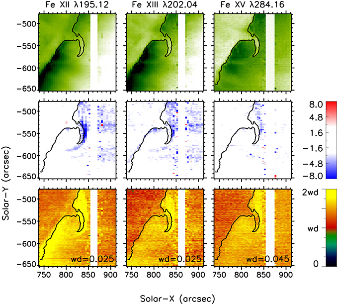
Figure 4. A subfield of the EIS raster scan starting from the left at 19:22 UT and finishing at 20:27 UT. Top row: EIS intensity (inverse log) for Fe XII 195.12 Å, Fe XIII 202.04 Å, and Fe XV 284.16 Å. Middle row: Doppler velocity maps for the three lines. Bottom row: Line widths of the given lines with the median line width (wd) given in each window. The white stripes are regions of missing data.

The top row of Figure 4 shows the region during the eruption. Cool plasma is now present along an arc as an absorption feature in the Fe XV 284.16 Å. The Doppler velocity maps show the eruption is strongly blue shifted for all three Fe lines throughout the eruption site as well as the region just north of the prominence. Additionally, the line widths for these regions are large compared to the pre-eruptive state. There is flowing material around the cavity but the structure of the cavity and prominence remain stable. During and after the eruption there is evidence for turbulence and heating within the cavity.

The chromospheric observations provide clues about the structure of the coronal cavity and overlying arcade when an eruption forces chromospheric plasma to flow over the cavity. Figure 5 provides an overview of the evolution of the eruption as observed in the IRIS Si IV 1400 Å SJI. The observations start with a prominence that appears in a stable configuration exhibiting minor plasma flows (top row). At 19:07 UT, the northern edge of the prominence brightens (middle row) and the bright plasma travels up and out along the outer edge of the prominence. Once the plasma reaches a certain height it cascades back toward the limb (bottom row). The cool plasma flows along an arc that mimics the shape of the prominence. The eruption is over by 21 UT when the system returns to its original state. Doppler velocity measurements of the chromospheric plasmas also show a predominantly blue-shifted flow. Figure 6 presents Si IV 1400 Å SJI with simultaneous spectra of Mg II 2796 Å and Si IV 1394 Å when the slit is just above the spicule region near the beginning of the eruption (top row) and near the end of the eruption (bottom row).

FIGURE 5

Figure 5. IRIS Si IV 1400 Å SJI.

FIGURE 6

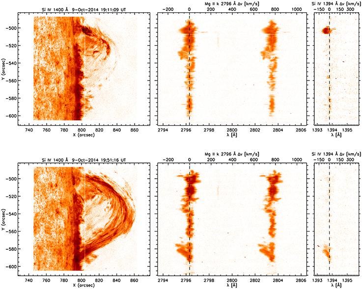
Figure 6. Left: IRIS Si IV 1400 Å. Middle: Mg II 2796 Å spectra. Right: Si IV 1394 Å spectra. In each spectra panel, the top axis x-axis is the Doppler velocity whose reference wavelength is marked by a dashed line.

Figure 7 and Supplementary Video 1 present high resolution SOT data showing striking details of the prominence and eruption. Initially, the prominence appears in a stable configuration with bi-directional plasma flows along the northern edge. This part of the prominence is highly stratified with the flows divided by regions with scant emission. Figures 7A,B show the prominence prior to the eruption with arrows pointing in the directions of plasma flow and a circle around the region where an intensity enhancement is seen in the minutes before the eruption. Figure 7C shows the time when the eruption starts. At this time, the bulk motion is in the direction of the arrow. As the eruption evolves, two bright ridges are prominent with regions of decreased intensity on either side. Figures 7D,E show that despite the upward bulk motion, the plasma does not move beyond the linear extrusion at the top of the prominence. In fact, the plasma flow is stalled as it encounters this barrier and the prominence experiences oscillatory motions in the regions around the two bright ridges. Eventually, the barrier is breached Figure 7F and plasma flows up along an arc, over the spine, exiting the FOV. Motions in the central regions of the prominence do not significantly change during or after the eruption. The motion slows and the plasma falls back down along the original trajectory path with some of the plasma flowing northward leaving the upper FOV Figure 7G. By the end of the observation run, the prominence is noticeably smaller Figure 7H.

FIGURE 7

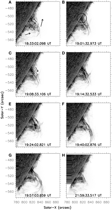
Figure 7. Hinode SOT Ca II H-line observations (inverse intensity) of the prominence during the eruption. Panels (A,B) shows the prominence prior to the eruption with the arrows (A) indicating plasma motions and the base of the eruption is circled in (B). Panels (C–E) show the initial phase of the eruption. The arrow points in the direction of the eruption. Panels (F,G) show the trajectory of the eruption and Panel (H) shows the prominence after the eruption.

Composite images of the X-ray emission with the SOT data are shown in Figure 8 and Supplementary Video 2. The X-ray data is scaled using an orange color table while the SOT image is a grayscale image. The time differences between the XRT images and nearest SOT image range from 1 to 30 s. Regions with low X-ray emission are set to be transparent with respect to the SOT data. Prior to the eruption, the prominence sits in a region with little X-ray emission. An arrow points to the eruption site where the X-ray emission increases just off the limb and the chromospheric plasma is ejected. After the pause in observations, the X-ray emission is strongest just outside the chromospheric plasma flows. A circle encompasses the bright X-ray emission that forms near the top of the prominence in Figure 8. These observations indicate that the eruption of the cool plasma observed by SOT was initiated by the incursion of hot plasma observed by XRT.

FIGURE 8

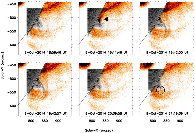
Figure 8. SOT inverse intensity (black and white) with XRT inverse intensity overlay (orange) of the prominence and cavity system. The arrow points to the increased X-ray emission at the start of the eruption. The circle outlines a region of increased X-ray emission after the eruption.

3.2. Model Results and Comparison to Observations

We construct several models with varying axial and poloidal fields and compare them with the observations. The model that best fit the observations has the correct magnetic field orientation to account for the observed plasma motions, Doppler velocities, and structures seen in XRT and the EUV data. Figure 9 presents the best model (Model 1) along with the potential field model and a highly twisted flux rope model (Model 2). The initial inserted flux rope for Model 1 has axial and poloidal fluxes of 2e20 Mx and 0 Mx/cm, respectively. Model 2 has the same initial axial flux and −2e10 Mx/cm poloidal flux. Both flux rope models have left helical twist and dextral chirality. After a 30,000-iteration relaxation, the models relax toward a force-free state.

FIGURE 9

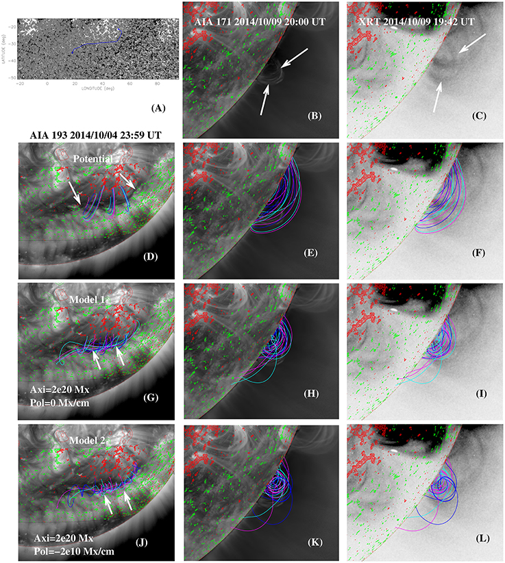
Figure 9. Magnetic field models constructed using the flux rope insertion method in comparison to observations. The models use combined LOS magnetograms observed by SDO/HMI from 2014 October 2 to October 5 at 19:00 UT. Panel (A) grayscale map of the LOS magnetic field with positive (white) and negative (black). The blue curve is the path of the flux rope and the circles indicate the footpoints of the flux tube. The bottom three rows show color contours of the magnetogram as positive (red) and negative (green) overlay on AIA 193 Å taken at 23:59 UT on October 4 (left), AIA 171 Å taken at 20:00 UT on October 9 (middle), and Hinode/XRT Be-thin taken at 19:42 UT on October 9 (right) with the color lines referring to selected magnetic field lines. Panels (B,C) AIA 171 Å observations and XRT Be-thin observations with arrows pointing out plasma motions and the coronal cavity. The color lines in the bottom rows refer to selected magnetic field lines from the potential field (D–F), Model 1 (G–I), and Model 2 (J–L).

Figure 9A shows a grayscale map of the LOS magnetic field with positive fields scaled white and negative fields black. The blue line shows the path of the inserted flux rope and the circles at the ends represent the footpoints of that flux rope. The path is selected to be along the PIL and the footpoints of the flux rope are embedded within patches of strong magnetic fields near the PIL. The same path is utilized for all of the models and a comparison of selected magnetic field lines (colored lines) for the three models are shown in Figures 9 D,G,J with an AIA 193 Å background image taken on 4 October 2014 at 23:59 UT. White arrows point to field lines that represent the orientation of the magnetic field.

The middle column of Figure 9 compares the three models rotated to the limb. The background image is an AIA 171 Å taken at 20:00 UT on 9 October 2014. Figure 9B shows the prominence with white arrows pointing to regions of plasma flow around the cavity. The right column compares the models with the background image as XRT thin-Be taken at 19:42 UT. Figure 9C shows the cavity with white arrows pointing to the regions of increased X-ray intensity around the coronal cavity. The bottom three rows of Figure 9 show selected field lines from the models in comparison to the Hinode/XRT and SDO/AIA observations.

Figure 9 shows that the observed arc-like filament structure is corresponding to the overlying magnetic field lines in the models, which are more sheared in Model 1 (Figure 9G) and nearly perpendicular to the filament channel for Model 2 (Figure 9J). Model 1 exhibits a weakly twisted flux rope structure after the relaxation, although the initial inserted flux bundle has no twist. This twist may be produced during the relaxation due to reconnection between the inserted sheared flux bundle and the overlying arcade. Model 1, shows magnetic field lines oriented in a way that could produce the observed Doppler velocities but the highly twisted flux rope, has magnetic field lines in the wrong orientation to account for the observed LOS Doppler velocities. The sheared overlying field lines can account for the aforementioned observed blue-shift flow in the overlying arcade. Therefore, we think that the weakly twisted flux rope fit the observations better. In comparison to the potential field model, and Model 2, the weakly twisted flux rope clearly shows a much better match to both the on-disk filament channel and the cavity observed on the limb by XRT.

One feature in the IRIS Si IV 1394 Å spectra is a persistent region with no emission on a portion of the on-disk scans. This region is outlined by two dotted lines in the top and bottom rows of Figure 10. This region persists throughout the observations but its location depends on the slit position. As the slit moves toward the limb, the region with no emission shifts northward until the slit reaches the limb. The Si IV emission just above the horizontal lines is also red-shifted relative to the average line centroid. The middle row of Figure 10 shows one of two slit positions that are almost exactly on the solar limb. The emission is strong in this region throughout the entire slit length. Once the slit clears the limb, the region of reduced emission is located over the prominence (bottom row) and the region continues to exhibit a redshift relative to the line average. There is also a noticeable decrease in the number of spicules near the base of the prominence. The orientation of the spicules in the peripheral regions of the prominence suggest they are curved away from the prominence.

FIGURE 10

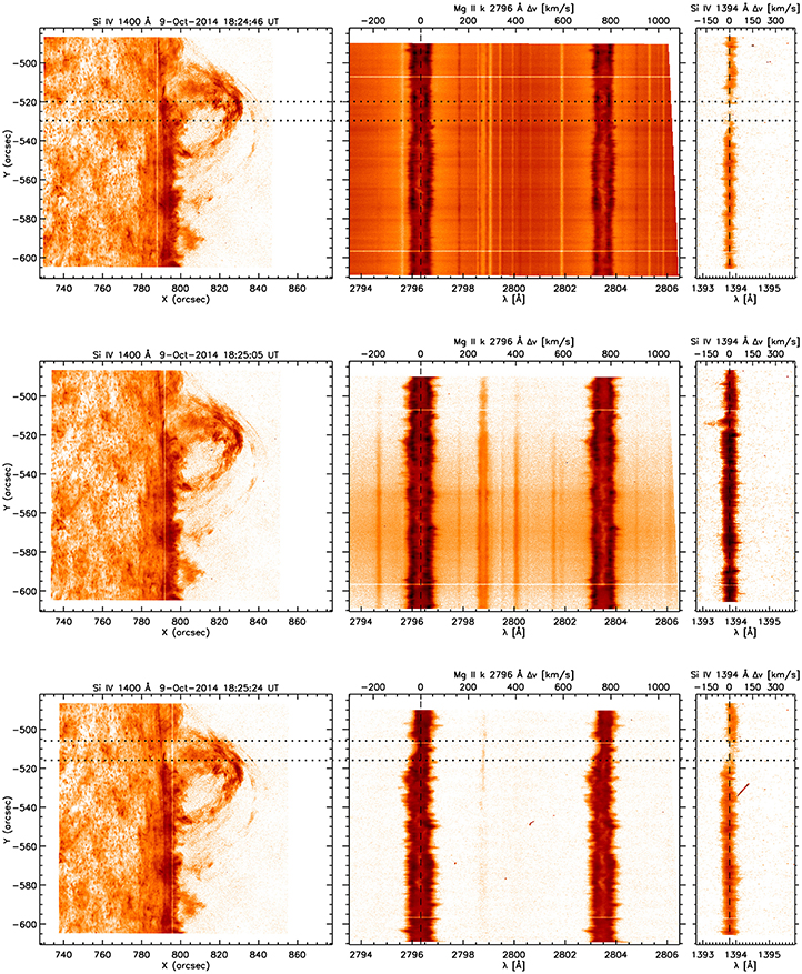
Figure 10. Left: IRIS Si IV 1400 Å with corresponding spectra for the Mg II 2796 Å (middle) and Si IV 1394 Å (right). The vertical dashed lines represent the rest wavelength. The horizontal dotted lines outline a region of decreased Si IV 1394 Å line intensity in the right image.

We compare the location of the depleted region observed in the IRIS Si IV 1394 Å spectra with the location of the PIL in Model 1. Figure 11 shows an IRIS Si IV 1400 Å SJ image, with the correct prominence orientation, along with contours (green/negative; red/positive) of the SDO/HMI LOS magnetic field model data. The region of reduced emission is located between the two white dotted lines. These are at the same location of the horizontal lines in the top row of Figure 10. A bipole sits near the region of reduced emission. The pink line is a small field line from Model 1 that crosses the PIL indicating its location. The right image shows the same location on the model data before it was rotated to the limb.

FIGURE 11

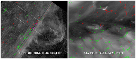
Figure 11. Left: IRIS Si IV 1400 Å rotated to its orientation on the limb taken at 18:24 UT on 9 October 2014. The white dashed lines indicate the region of reduced emission in the Si IV 1394 Å spectra shown in Figure 10. The green (negative) and red (positive) contours are the LOS photospheric magnetic field taken by SDO/HMI. The purple line crosses the PIL for this region. Right: AIA 193 Å with HMI magnetic field contours with the PIL at 23:59 UT on 4 October 2014.

To potentially constrain the model parameters we compare theoretical L/I measurements of Model 1 and the potential arcade with L/I CoMP measurements in Figure 12. The left image is CoMP L/I (log scale) observations of the prominence region. The prominence sits just above the limb (below 1.3 R_ʘ) so we cannot directly observe the prominence-cavity system in the CoMP data. However, some elements of the structure could still be present. The CoMP data does exhibit a linear decrease in intensity in a similar location to the potential arcade (middle panel) and Model 1 (right panel). The bright feature in the CoMP data is not seen in either of the models. The models do not contain information about other structures near the region so it is possible that the bright feature is not associated with the prominence. There are also minor differences between the potential arcade model and Model 1 far away from the disk. However, the CoMP data alone is not different enough to truly distinguish between the two models. Model 1 is a small flux rope embedded in a potential arcade, so at distances far from the flux rope, the L/I signatures are very similar to those of the potential arcade.

FIGURE 12

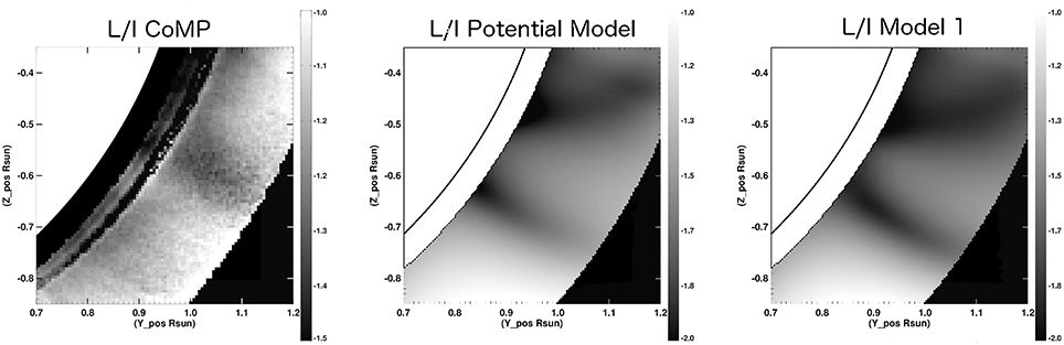
Figure 12. Left: CoMP QuickInvert L/I (log scale) observations of the region of interest at 21:13 UT on 9 October 2014. Middle: Potential field model results L/I with the CoMP field of view. Right: Model 1 results L/I with the same field of view.

4. Discussion

We present observations of a prominence and cavity system with an ensuing ancillary eruption that serves to highlight some of the topological features of the system. We find the prominence-cavity system maintains its structure during the event but heating is observed as an increase in X-ray emission around the coronal cavity and just above the prominence. Previous observational studies of bright X-ray emission within coronal cavities observed long-lived polar crown prominences where the bright core had already formed (Hudson et al., 1999; Reeves et al., 2012). The X-ray bright core always sits directly above the prominence although temperature structures found using EUV data (Schmit et al., 2009; Kucera et al., 2012) and white light studies find dynamic structures throughout the cavity (Habbal et al., 2010). The longevity of polar crown prominences, sometimes lasting several solar rotations, suggest a continuous heating process is needed to maintain the bright central emissions. Our observations suggest the heating inside the cavity is from a current sheet formed at a BPSS (Fan and Gibson, 2006). The BPSS forms a sheath or tunnel enclosing the dipped prominence field lines extending from the prominence footpoints in the photosphere, up into the cavity and would appear to be central to the cavity when viewed edge on. The BPSS can explain the steady-state X-ray emissions observed in long-lived polar crown prominences and it can explain the rapid increase in X-ray emission when a stable prominence system is disturbed.

The eruption causes oscillatory motions in the prominence near the eruption site but plasma motions within the central regions of the prominence do not change suggesting the inner prominence is structurally isolated from the eruption site. We model the prominence-cavity system as a flux rope situated under a coronal arcade. After testing several combinations of axial and poloidal fluxes we found the model that fit the observations best was that of a weakly twisted flux rope with dextral chirality.

The flux rope has opposite chirality than we would expect for a southern prominence Martin et al. (1994). The active regions north of the prominence have a positive (red) leading polarity whereas the prominence has the opposite (Figure 9). The dextral chirality is based on the comparison with the AIA emissions on the two sides of the filament channel. Through a statistical study Su et al. (2010) found that the emission on the two sides of the filament channel are asymmetric with one side showing bright and curved loops and the other side faint and straight emissions. They proposed that the bright curve features (on the southern side of filament channel for our case) are corresponding to the field lines that turn into the flux rope, and the straight faint features to the north, are the legs of the large overlying arcade. This idea was also confirmed by the magnetic field modeling in Su and van Ballegooijen (2012). The dextral flux rope model matches the direction of the observed bright curved feature on the southern side for our prominence, Figure 9G. The configuration also explains the trajectory of the erupting plasma as it flowed along magnetic field lines within the overlying arcade. The orientation of the arcade is such that any plasma flowing within the arcade would exhibit a predominantly blue-shifted LOS velocity when viewed on the limb.

The decreased emission of the Si IV 1394 Å spectra on the disk and in close proximity to the prominence coincides with the location of a bipole within the PIL of the model and thus we interpret it as evidence for a bald-patch underneath the prominence. A study by López Ariste et al. (2006) used vector magnetic fields to analyze bipolar regions within a filament channel. They found that at least four of the six bipolar regions exhibited a bald-patch topology forming photospheric dips where the horizontal component of the magnetic field points from a negative toward positive polarity. They concluded the observed magnetic field topology in the photosphere tends to support models of prominence based on magnetic dips located within weakly twisted flux tubes. Their underlying and lateral extensions form photospheric dips both within the channel and below barbs.

A comparison of the model with CoMP L/I observations were inconclusive as the prominence structure lies just above the limb but below the CoMP FOV. The flux rope for this model is small and embedded in a potential arcade. Far from the flux rope, the linear polarization will be similar to that of the overlying arcade. Ba̧k-Stȩślicka et al. (2016) performed a statistical study of quiescent coronal cavities observed with CoMP and found that coherent, often, ring-shaped, LOS Doppler velocity flows are common within cavities that possess a “lagomorphic” signature in the L/I polarization. The portion of the prominence we are studying is not oriented in the E-W direction and may not be in the best orientation to observe these signatures. Another reason that could account for the differences between the CoMP data and models is that our model only considers the local fields around the prominence. Differences observed in CoMP could be from other coronal structures.

Even if we could make linear polarization measurements up to the solar disk we would still have a difficult time distinguishing the L/I signatures of small flux ropes from those of the overlying potential arcade. The top row of Figure 13 compares the L/I signatures of a potential arcade model, Model 1 and Model 2. The linear polarization signatures are similar with varying differences in intensity. To observe the differences between the models we need to have V/I polarization measurements closer to the limb. The bottom row Figure 13 shows the V/I polarization measurements for the three models. The V/I can distinguish between the three models. Currently, V/I measurements are not practical as they require hours long integration times. However, an observatory that would be capable of making high resolution polarization measurements close to the solar limb is the proposed COronal Solar Magnetism Observatory (COSMO) (de Wijn et al., 2014). Future measurements from COSMO would clearly be very useful in determining magnetic structures of prominence-cavity systems.

FIGURE 13

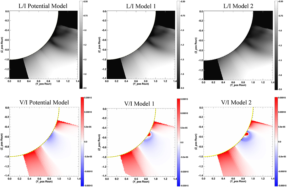
Figure 13. Top row: L/I (log scale) of the potential arcade model (left), weakly twisted flux rope (middle), and highly twisted flux rope (right). Bottom row: relative circular polarization (V/I) for the potential arcade model (left), weakly twisted flux rope (middle), and highly twisted flux rope (right).

Author Contributions

PJ performed the data analysis and document preparation. KR analyzed and interpreted the data. YS provided the NLFF models and documentation thereof.

Funding

PJ and KR are supported by under contract 80111112705 from Lockheed-Martin to SAO, contract NNM07AB07C from NASA to SAO, grant number NNX12AI30G from NASA to SAO, and contract Z15-12504 from HAO to SAO under a grant from AFOSR. YS is supported by the Youth Fund of Jiangsu No. BK20141043, the NSFC No. 11473071, and the “One Hundred Talent Program” of the Chinese Academy of Sciences.

Conflict of Interest Statement

The authors declare that the research was conducted in the absence of any commercial or financial relationships that could be construed as a potential conflict of interest.

Acknowledgments

IRIS is a NASA small explorer mission developed and operated by LMSAL with mission operations executed at NASA Ames Research center and major contributions to downlink communications funded by ESA and the Norwegian Space Centre. Hinode is a Japanese mission developed and launched by ISAS/JAXA, with NAOJ as domestic partner and NASA and STFC (UK) as international partners. It is operated by these agencies in co-operation with ESA and NSC (Norway). The authors acknowledge Dr. Adriaan van Ballegooijen for his valuable suggestions on the magnetic field modeling.

Supplementary Material

The Supplementary Material for this article can be found online at: https://www.frontiersin.org/article/10.3389/fspas.2016.00010

Footnotes

1. ^http://www.isas.jaxa.jp/home/solar/hinode_op/hop.php?hop=0264.

2. ^http://solarb.mssl.ucl.ac.uk:8080/eiswiki/Wiki.jsp?page=EISAnalysisGuide.

3. ^https://iris.lmsal.com/index.html.

4. ^http://www2.hao.ucar.edu/mlso/mlso-home-page.

5. ^http://www.hao.ucar.edu/FORWARD/.

References

Aulanier, G., Demoulin, P., van Driel-Gesztelyi, L., Mein, P., and Deforest, C. (1998). 3-D magnetic configurations supporting prominences. II. The lateral feet as a perturbation of a twisted flux-tube. Astron. Astrophys. 335, 309–322.

Google Scholar

Ba̧k-Stȩślicka, U., Gibson, S. E., and Chmielewska, E. (2016). Line-of-sight velocity as a tracer of coronal cavity magnetic structure. Front. Astron. Space Sci. 3:7. doi: 10.3389/fspas.2016.00007

CrossRef Full Text

Ba̧k-Stȩślicka, U., Gibson, S. E., Fan, Y., Bethge, C., Forland, B., and Rachmeler, L. A. (2013). The magnetic structure of solar prominence cavities: new observational signature revealed by coronal magnetometry. Astrophys. J. Lett. 770:L28. doi: 10.1088/2041-8205/770/2/L28

CrossRef Full Text

Berger, T. E., Slater, G., Hurlburt, N., Shine, R., Tarbell, T., Title, A., et al. (2010). Quiescent prominence dynamics observed with the hinode solar optical telescope. I. Turbulent upflow plumes. Astrophys. J. 716, 1288–1307. doi: 10.1088/0004-637X/716/2/1288

CrossRef Full Text | Google Scholar

Chae, J., Wang, H., Qiu, J., Goode, P. R., Strous, L., and Yun, H. S. (2001). The formation of a prominence in active region NOAA 8668. I. SOHO/MDI observations of magnetic field evolution. Astrophys. J. 560, 476–489. doi: 10.1086/322491

CrossRef Full Text | Google Scholar

Culhane, J. L., Harra, L. K., James, A. M., Al-Janabi, K., Bradley, L. J., Chaudry, R. A., et al. (2007). The EUV imaging spectrometer for hinode. Solar Phys. 243, 19–61. doi: 10.1007/s01007-007-0293-1

CrossRef Full Text | Google Scholar

De Pontieu, B., Title, A. M., Lemen, J. R., Kushner, G. D., Akin, D. J., Allard, B., et al. (2014). The Interface Region Imaging Spectrograph (IRIS). Solar Phys. 289, 2733–2779. doi: 10.1007/s11207-014-0485-y

CrossRef Full Text | Google Scholar

de Wijn, A. G., Tomczyk, S., and Burkepile, J. (2014). “A progress update for the coronal solar magnetism observatory for coronal and chromospheric polarimetry,” in Solar Polarization 7, Vol. 489 of Astronomical Society of the Pacific Conference Series, eds K. N. Nagendra, J. O. Stenflo, Q. Qu, and M. Samooprna (San Francisco), 323.

Dudík, J., Aulanier, G., Schmieder, B., Bommier, V., and Roudier, T. (2008). Topological departures from translational invariance along a filament observed by THEMIS. Solar Phys. 248, 29–50. doi: 10.1007/s11207-008-9155-2

CrossRef Full Text | Google Scholar

Fan, Y., and Gibson, S. E. (2006). On the nature of the X-ray bright core in a stable filament channel. Astrophys. J. Lett. 641, L149–L152. doi: 10.1086/504107

CrossRef Full Text | Google Scholar

Freeland, S. L., and Handy, B. N. (1998). Data analysis with the solarsoft system. Solar Phys. 182, 497–500. doi: 10.1023/A:1005038224881

CrossRef Full Text | Google Scholar

Gibson, S. E., Foster, D., Burkepile, J., de Toma, G., and Stanger, A. (2006). The calm before the storm: the link between quiescent cavities and coronal mass ejections. Astrophys. J. 641, 590–605. doi: 10.1086/500446

CrossRef Full Text | Google Scholar

Gibson, S. E., Kucera, T. A., White, S. M., Dove, J. B., Fan, Y., Forland, B. C., et al. (2016). FORWARD: a toolset for multiwavelength coronal magnetometry. Front. Astron. Space Sci. 3:8. doi: 10.3389/fspas.2016.00008

CrossRef Full Text | Google Scholar

Golub, L., Deluca, E., Austin, G., Bookbinder, J., Caldwell, D., Cheimets, P., et al. (2007). The X-Ray Telescope (XRT) for the hinode mission. Solar Phys. 243, 63–86. doi: 10.1007/s11207-007-0182-1

CrossRef Full Text | Google Scholar

Habbal, S. R., Druckmüller, M., Morgan, H., Scholl, I., Rušin, V., Daw, A., et al. (2010). Total solar eclipse observations of hot prominence shrouds. Astrophys. J. 719, 1362–1369. doi: 10.1088/0004-637X/719/2/1362

CrossRef Full Text

Hudson, H., and Schwenn, R. (2000). Hot cores in coronal filament cavities. Adv. Space Res. 25, 1859–1861. doi: 10.1016/S0273-1177(99)00618-3

CrossRef Full Text | Google Scholar

Hudson, H. S., Acton, L. W., Harvey, K. L., and McKenzie, D. E. (1999). A stable filament cavity with a hot core. Astrophys. J. Lett. 513, L83–L86. doi: 10.1086/311892

CrossRef Full Text | Google Scholar

Judge, P. G., and Casini, R. (2001). “A synthesis code for forbidden coronal lines,” in Advanced Solar Polarimetry – Theory, Observation, and Instrumentation, volume 236 of Astronomical Society of the Pacific Conference Series, ed M. Sigwarth (San Francisco), 503.

Kamio, S., Hara, H., Watanabe, T., Fredvik, T., and Hansteen, V. H. (2010). Modeling of EIS spectrum drift from instrumental temperatures. Solar Phys. 266, 209–223. doi: 10.1007/s11207-010-9603-7

CrossRef Full Text | Google Scholar

Kobelski, A. R., Saar, S. H., Weber, M. A., McKenzie, D. E., and Reeves, K. K. (2014). Calibrating data from the hinode/X-ray telescope and associated uncertainties. Solar Phys. 289, 2781–2802. doi: 10.1007/s11207-014-0487-9

CrossRef Full Text | Google Scholar

Kosugi, T., Matsuzaki, K., Sakao, T., Shimizu, T., Sone, Y., Tachikawa, S., et al. (2007). The hinode (solar-B) mission: an overview. Solar Phys. 243, 3–17. doi: 10.1007/s11207-007-9014-6

CrossRef Full Text | Google Scholar

Kucera, T. A., Gibson, S. E., Schmit, D. J., Landi, E., and Tripathi, D. (2012). Temperature and extreme-ultraviolet intensity in a coronal prominence cavity and streamer. Astrophys. J. 757, 73. doi: 10.1088/0004-637X/757/1/73

CrossRef Full Text | Google Scholar

Kuperus, M., and Raadu, M. A. (1974). The support of prominences formed in neutral sheets. Astron. Astrophys. 31:189.

Google Scholar

Lemen, J. R., Title, A. M., Akin, D. J., Boerner, P. F., Chou, C., Drake, J. F., et al. (2012). The Atmospheric Imaging Assembly (AIA) on the Solar Dynamics Observatory (SDO). Solar Phys. 275, 17–40. doi: 10.1007/s11207-011-9776-8

CrossRef Full Text | Google Scholar

Lin, H., Kuhn, J. R., and Coulter, R. (2004). Coronal magnetic field measurements. Astrophys. J. 613, L177–L180. doi: 10.1086/425217

CrossRef Full Text | Google Scholar

Liu, W., De Pontieu, B., Vial, J.-C., Title, A. M., Carlsson, M., Uitenbroek, H., et al. (2015). First high-resolution spectroscopic observations of an erupting prominence within a coronal mass ejection by the Interface Region Imaging Spectrograph (IRIS). Astrophys. Lett. 803, 85. doi: 10.1088/0004-637X/803/2/85

CrossRef Full Text | Google Scholar

López Ariste, A., Aulanier, G., Schmieder, B., and Sainz Dalda, A. (2006). First observation of bald patches in a filament channel and at a barb endpoint. Astron. Astrophys. 456, 725–735. doi: 10.1051/0004-6361:20064923

CrossRef Full Text | Google Scholar

Low, B. C., and Hundhausen, J. R. (1995). Magnetostatic structures of the solar corona. 2: The magnetic topology of quiescent prominences. Astrophys. Lett. 443, 818–836. doi: 10.1086/175572

CrossRef Full Text | Google Scholar

Mackay, D. H., Karpen, J. T., Ballester, J. L., Schmieder, B., and Aulanier, G. (2010). Physics of solar prominences: II-magnetic structure and dynamics. Space Sci. Rev. 151, 333–399. doi: 10.1007/s11214-010-9628-0

CrossRef Full Text | Google Scholar

Malherbe, J. M., and Priest, E. R. (1983). Current sheet models for solar prominences. I Magnetohydrostatics of support and evolution through quasi-static models. Astron. Astrophys. 123, 80–88.

Google Scholar

Martin, S. F. (1973). The evolution of prominences and their relationship to active centers (a review). Solar Phys. 31, 3–21. doi: 10.1007/BF00156070

CrossRef Full Text | Google Scholar

Martin, S. F. (1990). “Conditions for the formation of prominences as inferred from optical observations,” in IAU Colloq. 117: Dynamics of Quiescent Prominences, Vol. 363 of Lecture Notes in Physics, eds V. Ruzdjak and E. Tandberg-Hanssen (Berlin: Springer Verlag), 1–44.

Martin, S. F., Bilimoria, R., and Tracadas, P. W. (1994). “Magnetic field configurations basic to filament channels and filaments,” in NATO Advanced Science Institutes (ASI) Series C, Vol. 433 of NATO Advanced Science Institutes (ASI) Series C, eds R. J. Rutten and C. J. Schrijver (Dordrecht), 303.

Parenti, S. (2014). Solar prominences: observations. Living Rev. Solar Phys. 11, 1. doi: 10.12942/lrsp-2014-1

CrossRef Full Text | Google Scholar

Pneuman, G. W. (1983). The formation of solar prominences by magnetic reconnection and condensation. Solar Phys. 88, 219–239. doi: 10.1007/BF00196189

CrossRef Full Text | Google Scholar

Priest, E. (2014). Magnetohydrodynamics of the Sun. Cambridge, MA: Cambridge University Press.

Google Scholar

Priest, E. R., Hood, A. W., and Anzer, U. (1989). A twisted flux-tube model for solar prominences. I - General properties. Astrophys. Lett. 344, 1010–1025. doi: 10.1086/167868

CrossRef Full Text | Google Scholar

Rachmeler, L. A., Gibson, S. E., Dove, J. B., DeVore, C. R., and Fan, Y. (2013). Polarimetric properties of flux ropes and sheared arcades in coronal prominence cavities. Solar Phys. 288, 617–636. doi: 10.1007/s11207-013-0325-5

CrossRef Full Text | Google Scholar

Reeves, K. K., Gibson, S. E., Kucera, T. A., Hudson, H. S., and Kano, R. (2012). Thermal properties of a solar coronal cavity observed with the X-ray telescope on hinode. Astrophys. J. 746, 146. doi: 10.1088/0004-637X/746/2/146

CrossRef Full Text | Google Scholar

Rust, D. M., and Kumar, A. (1994). Helical magnetic fields in filaments. Solar Phys. 155, 69–97. doi: 10.1007/BF00670732

CrossRef Full Text | Google Scholar

Schmieder, B., Tian, H., Kucera, T., López Ariste, A., Mein, N., Mein, P., et al. (2014). Open questions on prominences from coordinated observations by IRIS, Hinode, SDO/AIA, THEMIS, and the Meudon/MSDP. Astron. Astrophys. 569:A85. doi: 10.1051/0004-6361/201423922

CrossRef Full Text | Google Scholar

Schmit, D. J., Gibson, S. E., Tomczyk, S., Reeves, K. K., Sterling, A. C., Brooks, D. H., et al. (2009). Large-scale flows in prominence cavities. Astrophys. J. 700, L96–L98. doi: 10.1088/0004-637X/700/2/L96

CrossRef Full Text | Google Scholar

Schou, J., Scherrer, P. H., Bush, R. I., Wachter, R., Couvidat, S., Rabello-Soares, M. C., et al. (2012). Design and ground calibration of the Helioseismic and Magnetic Imager (HMI) instrument on the Solar Dynamics Observatory (SDO). Solar Phys. 275, 229–259. doi: 10.1007/s11207-011-9842-2

CrossRef Full Text | Google Scholar

Schröter, E.-H., Vázquez, M., and Wyller, A. A. (eds.). (1987). The Role of Fine-Scale Magnetic Fields on the Structure of the Solar Atmosphere. Cambridge: Cambridge University Press.

Google Scholar

Smith, S. F. (1968). “The formation, structure and changes in filaments in active regions,” in Structure and Development of Solar Active Regions, Vol. 35 of IAU Symposium, ed K. O. Kiepenheuer, 267. doi: 10.1007/978-94-011-6815-1_42

CrossRef Full Text | Google Scholar

Stark, J.-L., and Murtagh, F. (2002). Astronomical Image and Data Analysis. Berlin: Springer.

Google Scholar

Su, Y., Surges, V., van Ballegooijen, A., DeLuca, E., and Golub, L. (2011). Observations and magnetic field modeling of the flare/coronal mass ejection event on 2010 april 8. Astrophys. J. 734, 53. doi: 10.1088/0004-637X/734/1/53

CrossRef Full Text | Google Scholar

Su, Y., and van Ballegooijen, A. (2012). Observations and magnetic field modeling of a solar polar crown prominence. Astrophys. J. 757, 168. doi: 10.1088/0004-637X/757/2/168

CrossRef Full Text | Google Scholar

Su, Y., van Ballegooijen, A., and Golub, L. (2010). Structure and dynamics of quiescent filament channels observed by hinode/XRT and STEREO/EUVI. Astrophys. J. 721, 901–910. doi: 10.1088/0004-637X/721/1/901

CrossRef Full Text | Google Scholar

Su, Y., van Ballegooijen, A., Lites, B. W., Deluca, E. E., Golub, L., Grigis, P. C., et al. (2009). Observations and nonlinear force-free field modeling of active region 10953. Astrophys. J. 691, 105–114. doi: 10.1088/0004-637X/691/1/105

CrossRef Full Text | Google Scholar

Su, Y., van Ballegooijen, A., McCauley, P., Ji, H., Reeves, K. K., and DeLuca, E. E. (2015). Magnetic structure and dynamics of the erupting solar polar crown prominence on 2012 march 12. Astrophys. J. 807, 144. doi: 10.1088/0004-637X/807/2/144

CrossRef Full Text | Google Scholar

Titov, V. S., and Démoulin, P. (1999). Basic topology of twisted magnetic configurations in solar flares. Astron. Astrophys. 351, 707–720.

Google Scholar

Tomczyk, S., Card, G. L., Darnell, T., Elmore, D. F., Lull, R., Nelson, P. G., et al. (2008). An instrument to measure coronal emission line polarization. Solar Phys. 247, 411–428. doi: 10.1007/s11207-007-9103-6

CrossRef Full Text | Google Scholar

Tsuneta, S., Ichimoto, K., Katsukawa, Y., Nagata, S., Otsubo, M., Shimizu, T., et al. (2008). The solar optical telescope for the hinode mission: an overview. Solar Phys. 249, 167–196. doi: 10.1007/s11207-008-9174-z

CrossRef Full Text | Google Scholar

Vaiana, G. S., Krieger, A. S., and Timothy, A. F. (1973). Identification and analysis of structures in the corona from X-Ray photography. Solar Phys. 32, 81–116. doi: 10.1007/BF00152731

CrossRef Full Text | Google Scholar

van Ballegooijen, A. A. (2004). Observations and modeling of a filament on the sun. Astrophys. J. 612, 519–529. doi: 10.1086/422512

CrossRef Full Text | Google Scholar

van Ballegooijen, A. A., and Martens, P. C. H. (1989). Formation and eruption of solar prominences. Atrophys. J. 343, 971–984. doi: 10.1086/167766

CrossRef Full Text | Google Scholar

van Ballegooijen, A. A., Priest, E. R., and Mackay, D. H. (2000). Mean field model for the formation of filament channels on the sun. Astrophys. J. 539, 983–994. doi: 10.1086/309265

CrossRef Full Text | Google Scholar

Vial, J.-C., and Engvold, O. (eds.). (2015). Solar Prominences, Vol. 415 of Astrophysics and Space Science Library. Springer International Publishing Switzerland.

Warren, H. P., Ugarte-Urra, I., Young, P. R., and Stenborg, G. (2011). The temperature dependence of solar active region outflows. Astrophys. J. 727, 58. doi: 10.1088/0004-637X/727/1/58

CrossRef Full Text | Google Scholar

Yoshimura, K., and McKenzie, D. E. (2015). Calibration of hinode/XRT for coalignment. Solar Phys. 290, 2355–2372. doi: 10.1007/s11207-015-0746-4

CrossRef Full Text | Google Scholar

Young, P. (2013). EIS Software Note No. 16, ver. 2.5. Available online at: http://solarb.mssl.ucl.ac.uk:8080/eiswiki/Wiki.jsp?page=EISAnalysisGuide