3D Global Coronal Density Structure and Associated Magnetic Field near Solar Maximum

1. Introduction

Solar coronal magnetic field is a major source of dynamics and thermodynamics of global coronal corona and transient coronal events including the coronal heating, solar flares, coronal mass ejections, and the solar wind. Its dynamics affects space weather processes that may impact Earth's magnetosphere and atmosphere and affect life on our planet. Thus, the knowledge of coronal magnetic field strength and topology represents one of major goals of the solar physics. Currently, coronal magnetic fields cannot directly measured. The major techniques that are currently used to derive the global magnetic structures of the solar corona represent indirect methods including potential field source surface (PFSS) models, non-linear force-free field (NLFFF) models and multi-dimensional magnetohydrodynamic (MHD) models of the global solar corona. These methods use solar photospheric scalar or vector magnetic field as input directly derived from photospheric magnetograms. However, as we discussed in Kramar et al. (2014), all these methods cannot adequately describe the dynamics of magnetic fields observed in the solar corona driven by current carrying structures. Moreover, they do not provide accurate information about the coronal thermodynamics, and thus cannot be used for modeling the coronal emission measures derived from extreme ultraviolet (EUV) observations. The MHD modeling of the solar corona provides a self-consistent time-dependent treatment of the plasma pressure, gravitational and magnetic forces, but are limited by approximations used for describing the coronal heating, and the uncertainties in the boundary conditions that are deduced from synoptic data. Thus, direct measurements of the coronal magnetic field remains one of the most reliable and challenging ways for characterization of solar coronal processes.

Direct measurement of the coronal magnetic field is the most challenging problem in observational solar physics. A major progress here was reached with the deployment of the Coronal Multichannel Polarimeter (CoMP) (Tomczyk et al., 2007, 2008). In order to interpret such type of data, a vector tomography method has been developed for 3D reconstruction of the global coronal magnetic field (Kramar et al., 2006, 2013), and recently, first 3D reconstruction of the global coronal magnetic field has been performed based on the CoMP data (Kramar et al., 2016).

Another, thought implicit but also based on coronal observations, way to reconstruct some global coronal magnetic field structures was investigated in Kramar et al. (2014). There we applied the tomography method that employs STEREO data to reconstruct 3D density of global solar corona and related it to the coronal magnetic field structure. This method was applied to characterize the solar corona over the Carrington rotation 2066 occurred during deep solar minimum for the range of coronal heights from 1.5 to 4 R_⊙ and provided description of the open/close magnetic field boundaries in the solar corona.

In this paper, we apply this method to study global solar coronal structures for the period of over the half of Carrington rotation 2131, which represents the case of solar maximum. Specifically, we use the STEREO/COR1 coronagraph data for half a solar rotation period during CR 2131 as input for the tomographic reconstruction of the 3D coronal electron density and the configuration of magnetic field associated with them. Our results are complemented by the 3D emissivity obtained by tomography method applied for the the STEREO Extreme Ultraviolet Imager (EUVI) data in the 195 Å band. We also compared the reconstructed 3D coronal structures with those implied by the PFSS model. In Section 4, we present the comparison of the 3D coronal structure near the solar maximum to those at deep solar minimum (CR 2066).

Two of the addressed problems we have analyzed are at which distance the global coronal magnetic field lines become radially directed and where are boundaries between closed and open magnetic field structures. An answer to this question is particularly important for predictions of the slow/fast solar wind and CME. Thus, it has been found that once erupted CME does not follow straight path but deflects according the global 3D coronal magnetic field (Xie et al., 2009; Kay et al., 2015). This complicates prediction of when and whether a CME encounter the Earth.

2. Methods

Because the solar corona is optically thin at visible and EUVI wavelengths, the observed flux in these spectral ranges is an integral of the emissivity along any line of sight (LOS). To our knowledge, tomography is the most effective method for three-dimensional (3D) reconstruction of optically thin objects based only on the LOS measurements made from multiple observing directions. The nice property of the method is that in its basic form it does not require any a priori knowledge about 3D properties of the object (except that it is optically thin) and its accuracy is generally depends on the quantity of measurements (number and coverage), their accuracy, a physical effect used in the LOS signal (i.e., diffraction limit, relation of emitting/absorbed light to the local property of the object, etc.), numerical inversion scheme (Natterer, 2001). This makes the method to be effectively used in many fields such as medical imaging, material structure research, geophysics, heliophysics and astrophysics (Boffin et al., 2001).

In this study, we apply the tomography method that employs STEREO data to reconstruct 3D density and EUVI emissivity of global solar corona. The method has been extensively described in Kramar et al. (2009, 2014). One of the most distinctive feature of this method is that it uses preconditioning which allows us to account for a large dynamical range of the coronal density values.

The relation of the 3D global coronal density and EUVI 195 Å emissivity to the properties of the coronal magnetic field has been investigated in Kramar et al. (2014). Particularly, it has been found that the position of maximal gradient of the density and 195 Å emissivity can be an indicator for the position of boundary between closed and open magnetic structures. In this study, we apply these methods to study 3D global solar coronal structures near maximum of the solar activity cycle and compare the reconstructed 3D corona with PFSS models.

Thought potential field models do not accurately describe the solar corona structure, they are very robust. One of the main adjustable parameters in PFSS models is location of the source surface after which the magnetic field becomes radially directed. There are several recent studies about consistency of PFSS model for various source surface distances with EUVI synoptic map and interplanetary magnetic field (Lee et al., 2011; Arden et al., 2014). Our approach on this matter is different. We compare PFSS models with 3D coronal electron density and related to it magnetic properties (open/closed magnetic field lines boundary).

For boundary conditions for the PFSS model (Altschuler and Newkirk, 1969), we used Carrington Rotation spherical harmonic transform coefficients from the National Solar Observatory (NSO) GONG data¹. We restricted the spherical harmonic polynomial coefficients in the PFSS model to 20th order which is sufficient for the extrapolation of the global corona.

3. 3D Coronal Structure during CR 2131

CR 2131 represents the period near maximum of solar activity cycle. In this study, we performed two types of tomographic reconstructions: 3D reconstruction of the electron density based on STEREO/COR1 data and 3D reconstruction for the EUVI 195 Å emissivity [units of photons s⁻¹ sr⁻¹ cm⁻³] based on STEREO/EUVI data.

In order to demonstrate a general structure of the coronal streamer belt for CR 2131, Figure 1 shows a spherical cross-section of the electron density at the heliocentric distance of 2 R_⊙ and Figure 2 shows a spherical cross-section of the EUVI 195 Å emissivity at the heliocentric distance of 1.1 R_⊙. Solid black and dashed red lines indicate the magnetic neutral line at corresponding heights for PFSS model with source surface located at 1.5 and 2 R_⊙, respectively. It was demonstrated earlier in Kramar et al. (2014) that the density maximum locations can serve as an indicator of current sheet position which is characterized by the magnetic neutral line. We can see in the Figures that coincidence of the derived from the PFSS models positions of the magnetic neutral line with the density concentrations is far from ideal.

FIGURE 1

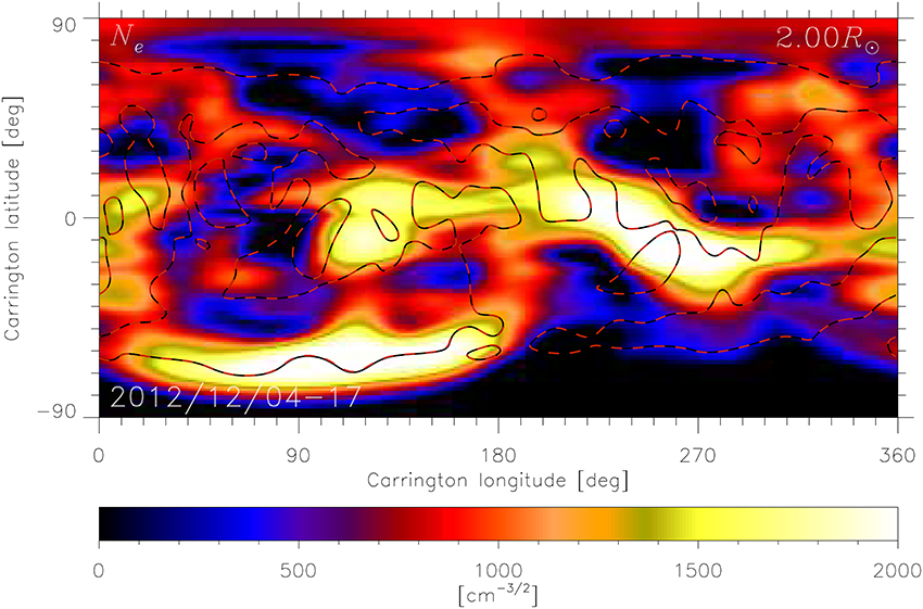
Figure 1. Spherical cross-section of the reconstructed electron density in square root scale at heliocentric distance of 2 R_⊙. The reconstruction is obtained by tomography based on COR-1 data obtained during December 4–17, 2012 (CR 2131). Solid black and dashed red lines indicate the magnetic neutral line in PFSS model with source surface located at 1.5 and 2 R_⊙, respectively.

FIGURE 2

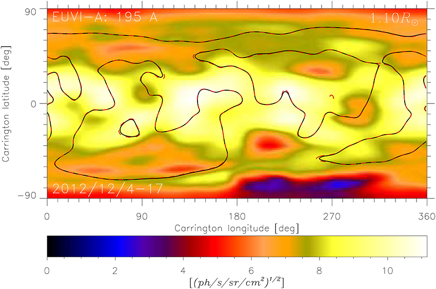
Figure 2. Spherical cross-section of the reconstructed 3D EUVI 195 Å emissivity in square root scale at heliocentric distances of 1.1 R_⊙. The reconstruction is obtained by tomography based on COR-1 data obtained during December 4–17, 2012 (CR 2131). Solid black and dashed red lines indicate the magnetic neutral line in PFSS model with source surface located at 1.5 and 2 R_⊙, respectively.

Figure 3 shows several meridional cross-sections of the electron density (range from 1.5 to 4 R_⊙) and EUVI 195 emissivity (range from 1.05 to 1.29 R_⊙). The figure with a set of all cross-sections is available in the Electronic Supplementary Material.

FIGURE 3

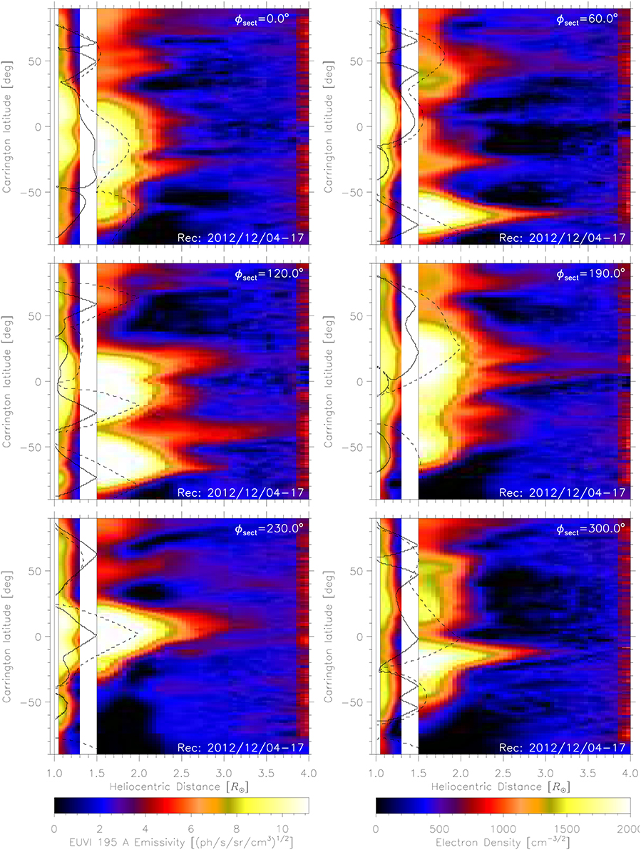
Figure 3. Reconstructions for CR 2131 based on COR1 data (electron density in the range from 1.5 to 4 R_⊙) and EUVI 195 Å data (emissivity in the range from 1.05 to 1.29 R_⊙). Carrington longitudes for cross-sections are shown at upper right corners. The figure with a set of all cross-sections is available in the Electronic Supplementary Material. The contour black lines show boundaries between open and closed magnetic-field structures for the PFSS models with Source Surface located at 1.5 and 2.0 R_⊙.

The black contour lines in Figure 3 show boundaries between open and closed magnetic-field structures in two PFSS models with Source Surface heliocentric distances [R_ss] at 1.5 and 2.0 R_⊙. The PFSS model with R_ss = 2.0 R_⊙ does not coincide with the derived positions of the streamer and pseudo-streamer as well as with the coronal hole positions indicated by the STEREO/EUVI 195 Å emissivity 3D reconstruction. The PFSS model with R_ss = 1.5 R_⊙ appears to fit the latter structures better.

It was previously demonstrated that the position of maximal gradient of the density and 195 Å emissivity can be an indicator for the position of boundary between closed and open magnetic structures Kramar et al. (2014). Therefore, in order to exhibit the possible real boundary positions, Figure 4 shows gradient of electron density and EUVI 195 emissivity, ∂N_e/∂θ and ∂ε₁₉₅/∂θ, for CR 2131 and for the same longitudinal cross-sections as in Figure 3. Both Figures 3, 4 demonstrate that the magnetic field configuration during CR 2131 has a tendency to become radially open at heliocentric distances below ~2.5 R_⊙. This is lower than corresponding distance during the deep solar minimum near CR 2066 (Kramar et al., 2014).

FIGURE 4

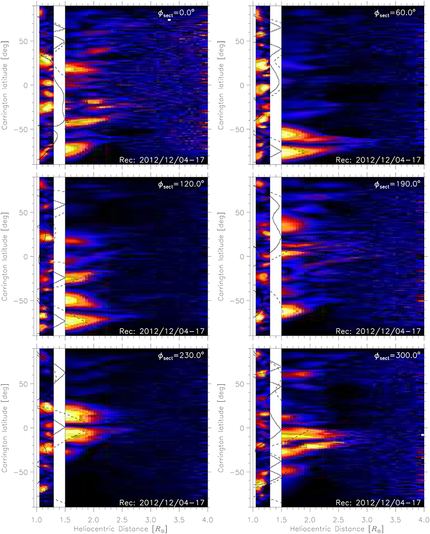
Figure 4. Longitudinal cross-sections of gradient of electron density and EUVI 195 emissivity, ∂N_e/∂θ and ∂ε₁₉₅/∂θ, for CR 2131. Carrington longitudes for cross-sections are shown at upper right corners. Color scales are different for different cross-sections to enhance the images. The contour black lines show boundaries between open and closed magnetic-field structures for the PFSS models with Source Surface located at 1.5 and 2.0 R_⊙.

Also, it should be noted that in Figures 3, 4 reconstructed streamers sometimes appear to slightly inclined toward the solar north. This could be because of stronger southern polar field. In fact, averaged over northern and southern hemispheres absolute values of magnetic field strength at 1.2 R_⊙ in the PFSS model with source surface at 2.0 R_⊙ are 0.59 and 1.04, respectively. The prevailing strength of the southern over the northern fields extends to higher distances. For example, the respective values at 1.9 R_⊙ are 0.06 and 0.11.

Figure 5 shows the radial profiles of the maximum (left panel) and average (right panel) electron density values at different heliocentric distances for CR 2066 (dashed green), 2112 (solid red), and 2131 (solid black). CR 2066 corresponds to deep solar minimum, while CR 2131 corresponds to period near solar maximum. The maximum values of coronal density mostly reflect the closed magnetic field structures represented by solar active regions, while average values include contributions from both open and closed field regions. The plot suggests that the maximum coronal density at the solar maximum is larger than the coronal density at two Carrington rotations representing the periods of lower magnetic activity. Specifically, at the lower boundary (at 1.8 R_⊙) of the reconstruction region the maximum density at solar maximum is more that twice greater than the maximum coronal density at solar minimum represented by CR 2066. This reflects the fact that the total unsigned magnetic flux that is structured in the form of coronal active regions during solar maximum is a factor of 2–3 greater than the emerging magnetic flux during solar minimum (Solanki et al., 2002). The average coronal density is a factor of 1.6 greater during solar maximum as compared to solar minimum, because it reflects the contribution of plasma emission formed in the diffuse corona as well as coronal active regions.

FIGURE 5

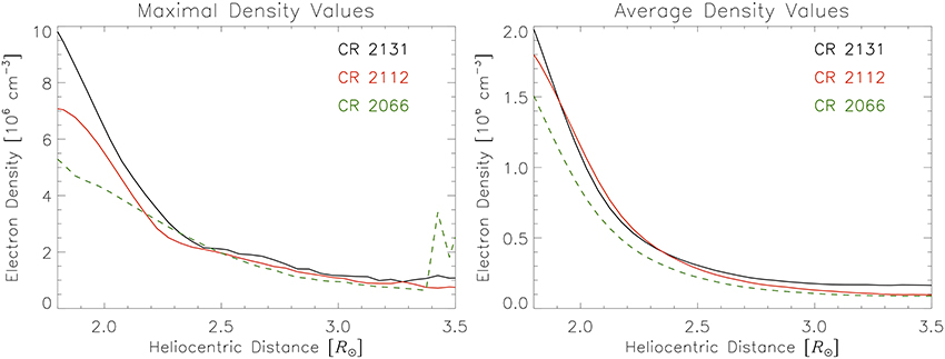
Figure 5. Maximal (left panel) and average over a spherical surface area (right panel) electron density values at different heliocentric distances for CR 2066 (dashed green), 2112 (solid red), and 2131 (solid black). CR 2066 corresponds to deep solar minimum, while CR 2131 corresponds to period near solar maximum.

Figure 6 shows the snapshot of the isosurface of coronal electron density value of 10⁶ cm⁻³ (in blue) for CR 2066 occurred at solar minimum (left) and CR 2131 at solar maximum (right). The corresponding movie showing the density isosurface over these two Carrington rotations are available provided in online version of the paper. The figure and the movie clearly demonstrate that the volume filling factor of the plasma with the density of 10⁶ cm⁻³ increases at solar maximum, which is consistent with Figure 5.

FIGURE 6

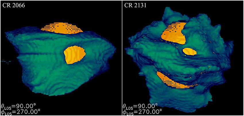
Figure 6. Isosurface of coronal electron density value of 10⁶ cm⁻³ (in blue) for CR 2066 (left) and 2131 (right). The orange sphere is located at 1.5R_⊙ just for scaling purpose. The movie demonstrating the isosurfaces for the whole longitudinal projection range is provided in online version of the paper.

4. Conclusion and Outlook

We applied the tomography method to STEREO-B/COR1 data to derive the reconstructions of the 3D global coronal electron density and EUVI 195 Å emissivity based on STEREO/COR1 and STEREO/EUVI observations near solar maximum represented by Carrington rotation CR 2131 (December 2012). We complemented the tomography with MHD simulations to obtain the open/closed magnetic field boundaries in the solar corona. Because the 3D reconstructions are based entirely on coronal data, these results could serve as an independent test and/or as an additional constraint for the models of the solar corona. Specifically, we used the PFSS model with different source surface distances as a test case for the reconstructed 3D electron density and EUVI 195 emissivity structures.

We have shown that magnetic field structures deviate significantly from the PFSS approximation as evident from the derived boundaries of open/closed field for both solar minimum (Kramar et al., 2014) and solar maximum. This suggests that potential field approximation for the low corona is not valid approximation when describing its large-scale structures. This discrepancy is most probably due to non-potential character of the solar coronal magnetic field. Although the fact that PFSS uses magnetograms collected over about a whole CR period while the tomographic reconstructions require observations over only half a CR period, the tomography provides more accurate description of the solar corona.

It is important to note that the magnetic field becomes radial at heights greater than 2.5R_⊙ during solar minimum, while its open up at heights below ~2.5R_⊙ during solar maximum.

Our studies also show that the average and the maximum electron densities in the low solar corona at heights ~1.8R_⊙ are about 2 times greater than that obtained during solar minimum. This is an important result that can be extrapolated to coronal densities of active and young solar-like stars. These stars show much greater levels of stellar activity in terms of at >10 times greater surface magnetic flux, up to 1000 times more luminous in X-rays and at least 10 times denser and hotter corona. These results open up an interesting opportunity to provide scaling of the electron density of the solar corona with different levels of magnetic activity traced by its X-ray luminosity and average surface magnetic flux. These scaling laws can be then used for characterization of stellar corona of active stars, which may provide insights on the nature of stellar coronal heating at various phases of their evolution.

Applied in this study method can also be used for verification of 3D global coronal vector magnetic field obtained by vector tomography based on coronal polarimetric observations (Kramar et al., 2016).

Author Contributions

MK developed the methods and wrote the codes. Also, MK led the calculations and contributed to the analysis of the results and writing the article. VA and HL assisted in calculations and contributed to the analysis of the results and writing the article.

Conflict of Interest Statement

The authors declare that the research was conducted in the absence of any commercial or financial relationships that could be construed as a potential conflict of interest.

Supplementary Material

The Supplementary Material for this article can be found online at: https://www.frontiersin.org/article/10.3389/fspas.2016.00025

Footnotes

1. ^http://gong.nso.edu/data/magmap/QR/mqc/

References

Altschuler, M. D., and Newkirk, G. (1969). Magnetic fields and the structure of the solar corona. I: methods of calculating coronal fields. Solar Phys. 9, 131–149. doi: 10.1007/BF00145734

CrossRef Full Text | Google Scholar

Arden, W. M., Norton, A. A., and Sun, X. (2014). A “breathing” source surface for cycles 23 and 24. J. Geophys. Res. (Space Phys.) 119, 1476–1485. doi: 10.1002/2013JA019464

CrossRef Full Text | Google Scholar

Boffin, H. M. J., Steeghs, D., and Cuypers, J. (eds.). (2001). Astrotomography, Volume 573 of Lecture Notes in Physics. Berlin: Springer Verlag.

Kay, C., Opher, M., and Evans, R. M. (2015). Global trends of CME deflections based on CME and solar parameters. Astrophys. J. 805:168. doi: 10.1088/0004-637X/805/2/168

CrossRef Full Text | Google Scholar

Kramar, M., Airapetian, V., Mikić, Z., and Davila, J. (2014). 3D coronal density reconstruction and retrieving the magnetic field structure during solar minimum. Solar Phys. 289, 2927–2944. doi: 10.1007/s11207-014-0525-7

CrossRef Full Text | Google Scholar

Kramar, M., Inhester, B., Lin, H., and Davila, J. (2013). Vector tomography for the coronal magnetic field. II. Hanle effect measurements. Astrophys. J. 775:25. doi: 10.1088/0004-637X/775/1/25

CrossRef Full Text | Google Scholar

Kramar, M., Inhester, B., and Solanki, S. K. (2006). Vector tomography for the coronal magnetic field. I. Longitudinal Zeeman effect measurements. Astron. Astrophys. 456, 665–673. doi: 10.1051/0004-6361:20064865

CrossRef Full Text | Google Scholar

Kramar, M., Jones, S., Davila, J., Inhester, B., and Mierla, M. (2009). On the tomographic reconstruction of the 3D electron density for the solar corona from STEREO COR1 data. Solar Phys. 259, 109–121. doi: 10.1007/s11207-009-9401-2

CrossRef Full Text | Google Scholar

Kramar, M., Lin, H., and Tomczyk, S. (2016). Direct observation of solar coronal magnetic fields by vector tomography of the coronal emission line polarizations. Astrophys. J. Lett. 819:L36. doi: 10.3847/2041-8205/819/2/L36

CrossRef Full Text | Google Scholar

Lee, C. O., Luhmann, J. G., Hoeksema, J. T., Sun, X., Arge, C. N., and de Pater, I. (2011). Coronal field opens at lower height during the solar cycles 22 and 23 minimum periods: IMF comparison suggests the source surface should be lowered. Solar Phys. 269, 367–388. doi: 10.3847/2041-8205/819/2/L36

CrossRef Full Text | Google Scholar

Natterer, F. (2001). The Mathematics of Computerized Tomography. Classics in Applied Mathematics. Philadelphia, PA: Society for Industrial and Applied Mathematics, SIAM monographs on mathematical modeling and computation.

Google Scholar

Solanki, S. K., Schüssler, M., and Fligge, M. (2002). Secular variation of the Sun's magnetic flux. Astron. Astrophys. 383, 706–712. doi: 10.1051/0004-6361:20011790

CrossRef Full Text | Google Scholar

Tomczyk, S., Card, G. L., Darnell, T., Elmore, D. F., Lull, R., Nelson, P. G., et al. (2008). An instrument to measure coronal emission line polarization. Solar Phys. 247, 411–428. doi: 10.1007/s11207-007-9103-6

CrossRef Full Text | Google Scholar

Tomczyk, S., McIntosh, S. W., Keil, S. L., Judge, P. G., Schad, T., Seeley, D. H., et al. (2007). Alfvén waves in the solar corona. Science 317:1192. doi: 10.1126/science.1143304

PubMed Abstract | CrossRef Full Text | Google Scholar

Xie, H., St. Cyr, O. C., Gopalswamy, N., Yashiro, S., Krall, J., Kramar, M., et al. (2009). On the origin, 3D structure and dynamic evolution of CMEs near solar minimum. Solar Phys. 259, 143–161. doi: 10.1007/s11207-009-9422-x

CrossRef Full Text | Google Scholar