MHD Simulation of Prominence-Cavity System

1. Introduction

Solar filaments and prominences are observed to be a major precursor of coronal mass ejections (CMEs) (e.g., Webb and Hundhausen, 1987). When observed in white light or EUV above the limb viewed nearly along their lengths, they often display a prominence-cavity system with a relatively dark cavity surrounding the lower central prominence (see review by Gibson, 2015). EUV observations of prominence-cavity systems have also shown substructures within the cavities with “U”-shaped prominence “horns” extending from the prominence, enclosing a central “cavity” or “void” on top of the prominence, see e.g., Figures 8, 12 in Gibson (2015) and Figure 2c in Su et al. (2015). The first 3D MHD simulations of prominence formation in a stable equilibrium coronal magnetic flux rope were carried out by Xia et al. (2014); Xia and Keppens (2016). With the use of adaptive grid refinement and including the chromosphere as the lower boundary, their 3D simulations obtained a prominence-cavity system with the prominence showing fine-scale, highly dynamic fragments, reproducing many observed features seen in SDO/AIA observations.

Recently, Fan (2017) (hereafter F17) and Fan (2018) (hereafter F18) have carried out 3D MHD simulations of prominence forming coronal flux ropes under coronal streamers, with the flux rope evolving from quasi-equilibrium to onset of eruption, leading to a CME with associated prominence eruption. In those simulations, a significantly twisted, longitudinally extended flux rope is built up in the corona under a pre-existing coronal streamer solution by an imposed flux emergence at the lower boundary. During the quasi-static evolution of the emerged flux rope, cool prominence condensations are found to form in the dips of the significantly twisted field lines due to the radiative instability driven by the optically thin radiative cooling of the relatively dense plasma in the emerged dips. In the prominence-forming flux rope simulation in F18 (labeled as the “PROM” simulation in that paper), we find that the prominence weight is dynamically important and can suppress the onset of the kink instability and hold the flux rope in quasi-equilibrium for a significantly longer period of time, compared to a case without prominence formation. We also find the formation of a cavity surrounding the prominence, and substructures inside the cavity such as prominence “horns” and a central “cavity” on top of the prominence. However in the simulations in F18, a pre-existing streamer solution (the “WS” solution in F17) with a wide mean foot-point separation of the arcade field lines are used and the corresponding potential field has a slow decline with height. As a result, we obtained a prominence and cavity that extend to rather large heights that are larger than typically observed before the onset of eruption. Here we extend the work of F17 and F18 by modeling the prominence-forming flux rope under a pre-existing coronal streamer with a significantly narrower mean foot-point separation for its closed arcade field lines. We find the formation of a prominence-cavity system with the heights for the prominence and the cavity that are more in accordance with those of the typically observed quiescent prominence-cavity systems. We carry out a more detailed analysis of the characteristics of the 3D magnetic fields comprising the different features of the prominence-cavity system. We also find that the flux rope begins to erupt at a significantly lower height, consistent with the onset of the torus instability, and results in a fast CME with an associated prominence eruption that shows a kinked morphology.

2. Model Description

For the MHD simulation presented in this paper, we use the same numerical MHD model described in detail in F17. The readers are referred to that paper's sections 2 and 3.1 for the description of the equations solved, the numerical code, and the initial and boundary conditions for the simulation set-up. As a brief overview, we use the “Magnetic Flux Eruption” (MFE) code to solve the set of semi-relativistic MHD equations [Equations (1–6) in F17] in spherical geometry, with the energy equation explicitly taking into account the non-adiabatic effects of an empirical coronal heating (which depends on height only), optically thin radiative cooling, and the field-aligned electron heat conduction. The inclusion of these non-adiabatic affects allow for the development of the radiative instability that leads to the formation of prominence condensations in the coronal flux rope as shown in the simulations of F17 and F18. The simulation domain is in the corona, ignoring the photosphere and chromosphere layers, with the lower boundary temperature (T = 5 × 10⁵ K) set at the base of the corona, but with an adjustable base density (and hence base pressure) that depends upon the downward heat conduction flux to crudely represent the effect of chromospheric evaporation (Equations (17, 18) and the associated descriptions in F17). The radiative loss function Λ(T) used for the radiative cooling in Equation (13) in F17 is the “actual” curve shown in Figure 1 of F17 (also the same as the “PROM” case in F18). As described in F17, the radiative loss function used is modified to suppress cooling for T ≤ 7 × 10⁴ K, so that the smallest pressure scale height of the coolest plasma that can form does not go below two grid points given our simulation resolution. In the following we describe the specific changes that have been made in the set-up of the current simulation.

FIGURE 1

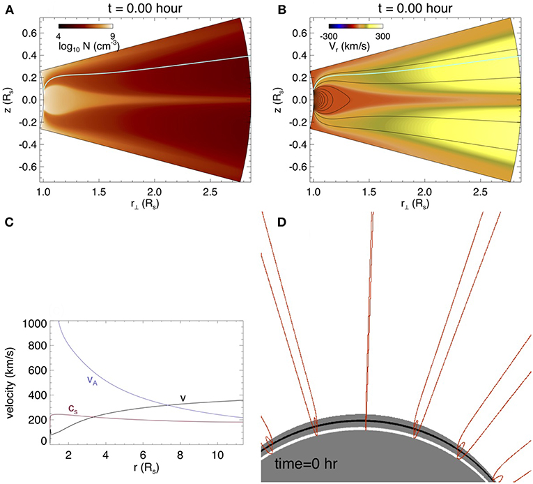
Figure 1. The relaxed 2D quasi-steady streamer solution for the initial state. (A) shows the cross-section density, (B) shows the cross-section radial velocity over-plotted with magnetic field lines, (C) shows the parallel velocity V, the Alfvén speed V_A, and sound speed C_S along an open field line [marked as the green line in (A,B)] in the ambient solar wind. (D) shows a 3D view of the initial streamer field lines in the simulation domain with the lower boundary color showing the normal flux distribution of the initial bipolar bands.

The empirical coronal heating used in this simulation is modified to use two exponentially decaying (with height) components instead of just one used in F17, i.e., we change Equation (14) in F17 to the following:

$\begin{array}{rc}H=\frac{F_1}{L_1}\frac{R_s^2}{r^2}exp\left[-(r-R_s)/L_1\right]+\frac{F_2}{L_2}\frac{R_s^2}{r^2}exp\left[-(r-R_s)/L_2\right]& \left(1\right)\end{array}$

where the input energy flux densities for the two components are $F_1=F_2=5\times 10^5\text{ergs}{\text{cm}}^{-2}{\text{s}}^{-1}$, and the decay lengths are $L_1=5\times 10^{10}$ cm and $L_2=2.5\times 10^9$ cm, r is the radial distance to the center of the sun and R_s denotes the solar radius. The first much more extended component is aimed to heat and accelerate the background solar wind and open up the ambient coronal magnetic field. The second more spatially confined heating is aimed to enhance the heating near the base to enhance the base pressure and plasma inflow into the corona, which promotes the formation of prominence condensations in the emerged flux rope.

As described in section 3.1 of F17, we first initialize a 2D quasi-steady solution of a coronal steamer with an ambient solar wind in a longitudinally extended (in ϕ) spherical wedge domain. We use the same simulation domain (with r∈[R_s, 11.47R_s], θ∈[75°, 105°], and ϕ∈[−75°, 75°], where R_s is the solar radius) and the grid as those for the “WS-L” (wide-streamer/long flux-rope) simulation in F17 (also the “PROM” simulation in F18). However, we use the initial normal flux distribution of a narrow bipolar pair of bands on the lower boundary as that for the NS (narrow-streamer) solution in F17 (see Figure 2b in F17), and increase the field strength by a factor of two. We obtain the relaxed 2D quasi-steady streamer solution for the initial state as shown in Figure 1. The cross-sections (panels a,b) of the initial state show a dense helmet dome of closed magnetic field approximately in static equilibrium, surrounded by an ambient open field region with a solar wind outflow with flow speed that accelerates to supersonic and super Alfvénic speed (see panel c). A 3D view of the initial streamer field lines in the simulation domain is shown in Figure 1D.

Into this initial streamer field, we then impose at the lower boundary the emergence of a twisted magnetic torus by specifying an electric field as described in F17 (see Equations (19–22) and the associate description in F17). The specific parameters for the driving emerging torus (see the definitions of the parameters in F17) used for the present simulation are: the minor radius a = 0.04314R_s, twist rate per unit length q/a = −0.0166 rad Mm⁻¹, major radius $R^{\prime }=0.75R_s$, axial field strength $B_{t}a/R^{\prime }=106$ G, and the driving emergence speed v₀ = 1.95 km/s. The driving flux emergence at the lower boundary is stopped when the total twist in the emerged flux rope reaches about 1.76 winds of field-line twist between the two anchored ends.

We note that the present simulation and the PROM simulation in F18 are similar in the driving flux emergence, where a long flux rope of similar total twist is driven into the corona. The essential difference is that the pre-existing arcade field in the streamer of the present simulation has a significantly narrower foot-point separation and a stronger foot-point field strength (compare Figure 1B in this paper and Figure 2b in F18). The mean foot-point separation in the present case is 0.13R_s compared to 0.24R_s for that in the PROM simulation in F18. The narrower foot-point separation results in a faster decline of field strength with height for the corresponding potential field in the present case. With a stronger arcade foot-point field strength, we expect a stronger confinement of the emerging flux rope to a lower height, and hence smaller cavity and prominence heights, improving upon the PROM case in F18, in which the cavity and prominence heights obtained are too high compared to the typical observed values. Furthermore, the stronger field strength lower down and the faster decline with height of the corresponding potential field are expected to have significant effects on the height for the onset of the torus instability and the acceleration of the erupting flux rope as shown in previous simulations by Török and Kliem (2007).

3. Simulation Results

3.1. Overview of Evolution

Figures 2a–f show snapshots of the 3D coronal magnetic field lines during the course of the evolution of the emerged coronal flux rope, from the quasi-static phase to the onset of eruption. The field lines shown in the snapshots are selected as follows. A set of field lines from a set of fixed foot points in the pre-existing bipolar bands are traced as the red field lines (same field lines as those traced in Figure 1D for the initial state). For the representative field lines in the emerged flux rope, we trace field lines from a set of tracked foot points at the lower boundary that connect to a set of selected field lines of the subsurface emerging torus and color the field lines (green, cyan, and blue) based on the flux surfaces of the subsurface torus. Figures 2g–l show the synthetic SDO/AIA EUV images in 304 Å channel as viewed from the same line of sight (LOS) corresponding to the snapshots shown in Figures 2a–f. The synthetic AIA images are computed by integrating along individual line-of-sight (LOS) through the simulation domain:

$\begin{array}{rc}{I}_{\text{channel}}={\displaystyle \int }{n}_e^2(l)f_{\text{channel}}(T(l))dl,& \left(2\right)\end{array}$

where l denotes the length along the LOS through the simulation domain, I_channel denotes the integrated emission intensity at each pixel of the image in units of DN/s/pixel (shown in LOG scale in the images), “channel” denotes the AIA wavelength channel (which is 304 Å in the case for Figures 2g–l), n_e is the electron number density, and f_channel(T) is the temperature response function that takes into account the atomic physics and the properties of the AIA channel filter. We obtain the temperature dependent function f_channel(T) for the individual filters using the SolarSoft routine get_aia_response.pro. The response function for the AIA 304 Å channel peaks at the temperature of about 8 × 10⁴K, thus the synthetic emission images show where the cool prominence plasma condensations form in the flux rope. For the LOS integration, we also have assumed that the prominence condensations are “optically thick” such that when the LOS reaches a plasma where both the temperature goes below 7.5 × 10⁴ K and the number density is above 10⁹cm³, we stop the integration for that LOS assuming the emission from behind the plasma is blocked and does not contribute to the integrated emission for the LOS. Figure 3 shows the evolution of the total magnetic energy E_m, the total kinetic energy E_k, the rise velocity at the apex of the axial field line of the emerged flux rope, and the temporal evolution of the cool prominence mass in the corona evaluated as the total mass with temperature below 10⁵ K. From t = 0 to 8.42 h, E_m increases as the emergence of a twisted magnetic torus is imposed at the lower boundary, and a long coronal flux rope is built up quasi-statically, confined by the coronal streamer as can be seen in the snapshot in Figure 2a at t = 8.42 h . The emergence is stopped at t = 8.42 h at which time the total field line twist about the axial field line of the emerged flux rope reaches about 1.76 winds between the anchored ends. This twist is above the critical value (about 1.25 winds) for the onset of the kink instability for a simple 1-dimensional cylindrical line-tied force-free flux rope (Hood and Priest, 1981). However subsequently, the flux rope is found to settle into a quasi-static rise phase over a long period of time (corresponding to about 131 Alfvén crossing times along the axis), from t = 8.42 h to about t = 17 h, with nearly zero acceleration (Figure 3B). We find that a long extended prominence has formed in the emerged flux rope (see Figures 2g,h), with the prominence condensations in the dips of the twisted field lines. In the PROM simulation in F18, it is shown that the cool prominence condensations form due to the development of the radiative instability of the dense plasma in the dips after their emergence. Here in the present case we find that cool prominence condensations begin to form even earlier in the flux emergence, soon after the apex of the flux rope emerges, as dense plasma is pushed into the corona with the stronger flux rope field. However these earlier forming condensations are unsteady and drain down as the flux rope emergence continues, and later more stable condensations form in the dips of the emerged field lines as in the PROM case. In Figure 3C we see large temporal fluctuations of the cool prominence mass during the early phase of the flux emergence. After the emergence is stopped (marked by the vertical dotted line in Figure 3), the prominence mass shows both a phase of continued increase and then a gradual decrease during the quasi-static phase (from t = 8.42 h to about t = 17 h). However this change from an increase of prominence mass to a decline does not seem to be associated with any significant change in the rise velocity in the quasi-static phase. During this quasi-static rise period the magnetic energy decreases slowly (see Figure 3) due to the continued magnetic reconnections, until about t = 17 h when it reaches a height of about r = 1.17R_s, where the flux rope begins a monotonic acceleration (see Figure 4A) and erupts subsequently with a sharp decrease of the magnetic energy and a significant increase of the kinetic energy (see Figure 3A). Figure 4 shows that the height (marked by the vertical dotted line) at which the flux rope begins to accelerate monotonically (see panel a) corresponds to the height at which the decay rate of the corresponding potential field reaches a magnitude of about 1.6 (see panel b), which exceeds the critical decline rate of about 1.5 for the onset of the torus instability for a toroidal flux rope (e.g., Kliem and Török, 2006). Thus in the present case, the onset of eruption is compatible with the onset of the torus instability. We find that in the present simulation, the flux rope begins to erupt at a significantly lower height (at about r = 1.17R_s) compared to that (at about r = 1.6R_s) in the PROM simulation in F18. This is because the arcade field lines in the pre-existing streamer of the PROM simulation have a significantly wider mean foot-point separation and hence the corresponding potential field declines with height significantly more slowly, where the magnitude of the decay rate remains below 1.5 until about r = 1.3R_s in that case.

FIGURE 2

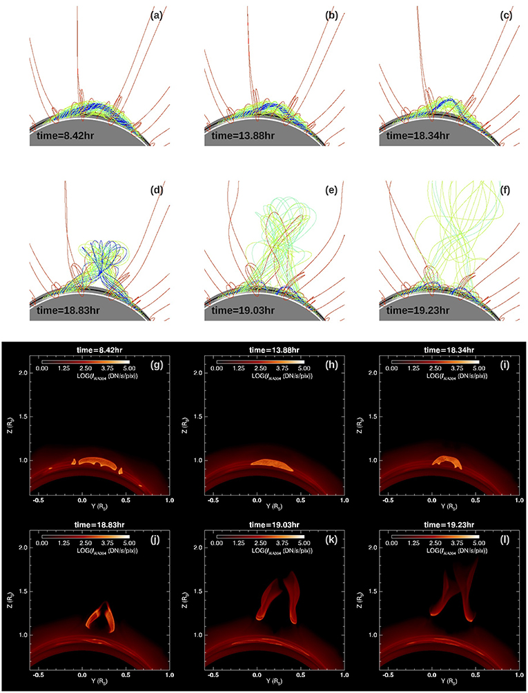
Figure 2. (a–f) show a sequence of snapshots of the 3D magnetic field lines through the course of the evolution of the emerged coronal flux rope, and (g–l) show the corresponding synthetic SDO/AIA EUV images in 304 Å channel from the same perspective view.

FIGURE 3

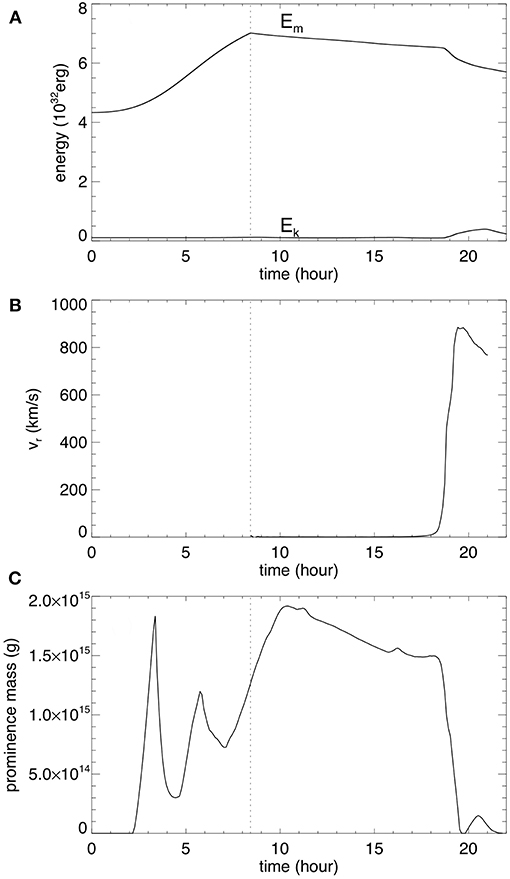
Figure 3. (A) The evolution of the total magnetic energy E_m and total kinetic energy E_k, (B) the evolution of the rise velocity at the apex of the axial field line of the emerged flux rope, and (C) the evolution of the cool prominence mass in the corona evaluated as the total mass with temperature below 10⁵ K.

FIGURE 4

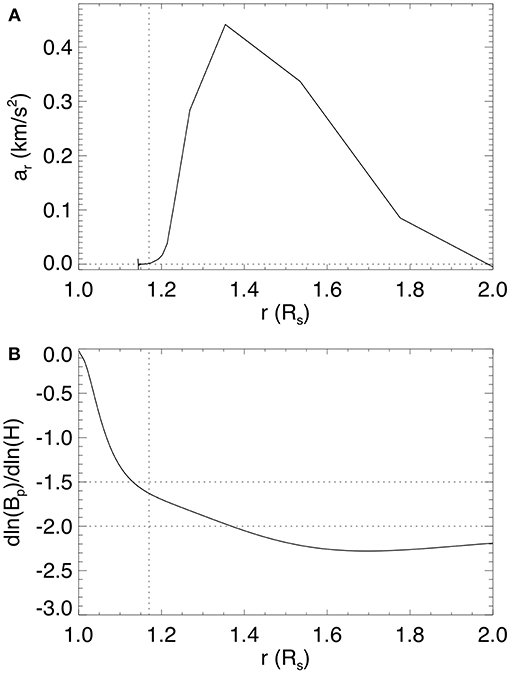
Figure 4. (A) Acceleration at the apex of the flux rope's axial field line as a function of its height position, and (B) the decay rate of the corresponding potential magnetic field strength B_p with height H (above the surface) when the emergence is stopped (after which the lower boundary normal magnetic flux distribution and the corresponding potential field remain fixed).

Although the confining potential field in the present case declines with height more steeply, it is stronger lower down and hence the flux rope and the prominence during the quasi-static phase reach significantly lower heights compared to the PROM case, and the flux rope field strength is also significantly stronger. The peak Alfvén speed in the central flux rope cross-section in the present case reaches about 4, 100 km/s with a peak field strength of about 24G, compared to the peak Alfvén speed of about 1, 500 km/s and peak field strength of about 9G in the PROM case during the quasi-static stage. The stronger flux rope field strength causes the prominence-carrying field to be much closer to force-free compared to the PROM case, as shown in Figure 5 compared to Figure 6 in F18. Figure 5 shows that the net Lorentz force (the green curve in the top panel) that balances the gravity force (the red curve) of the prominence is at most about 0.1 of either the magnetic tension or magnetic pressure gradient. In contrast in the PROM case in F18, there is a significant net Lorentz force to balance the prominence gravity that is comparable to the magnetic tension, i.e., the prominence carrying fields in the flux rope is significantly non-force-free. In the present case however, the magnetic field is close to force-free throughout the flux rope, even for the prominence-carrying field. Thus we do not see a significant variation of the rise velocity during the quasi-static phase in response to the growth or decline of prominence condensation mass as found above, and the onset of eruption is consistent with the onset of the torus instability. The stronger flux rope field strength in the present case also produces a stronger acceleration and a higher peak velocity of the erupting flux rope. In the present case the flux rope is found to accelerate to a peak velocity of nearly 900 km/s (see Figure 3B), compared to the peak velocity of about 600 km/s reached in the PROM simulation (see Figure 4B in F18). However, the ratio of the peak velocity over the peak Alfvén speed of the flux rope is found to be lower (0.22) in the present case compared to the PROM case (0.4).

FIGURE 5

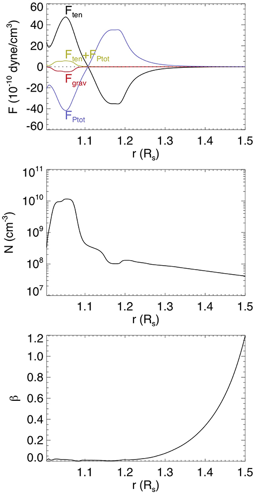
Figure 5. Several radial forces (Top), density (Middle), and plasma-β (the ratio of gas pressure to magnetic pressure) (Bottom) along the central vertical line through the middle of the flux rope in Figure 2b. The radial forces shown in the top panel are the magnetic tension force F_ten (black curve), the total pressure gradient force F_Ptot (blue curve), which is predominantly the magnetic pressure gradient (because of the low plasma-β) as shown in the bottom panel), the sum F_ten+F_Ptot (green curve), which is approximately the net Lorentz force, and the gravity force of the plasma F_grav (red curve). as a function of height.

Although the onset of eruption in the present simulation is consistent with the onset of the torus instability, because of the significant total twist in the emerged flux rope, the erupting flux rope shows significant rotational motion and a kinked morphology as can be seen in Figures 2d–f. The associated erupting prominence also shows a kinked morphology (see Figures 2j–l). The rotation of the erupting prominence is more clearly seen from the view shown in Figure 6, where the flux rope is viewed nearly along its length. We can clearly see the writhing motion of the erupting prominence due to the writhing motion of the hosting flux rope.

FIGURE 6

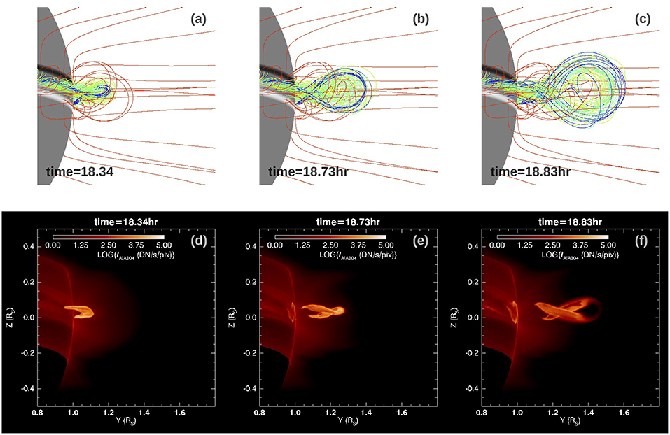
Figure 6. Successive snapshots of the erupting flux rope field lines (a–c) and the corresponding synthetic AIA 304 Å images (d–f), viewed with a LOS that is close to aligned with the length of the flux rope. They show the writhing motion of the flux rope and the associated erupting prominence.

We also note that two brightening ribbons are visible in the AIA 304 Å images (Figures 6e,f) on the lower boundary under the erupting prominence. The brightening ribbons correspond to the foot points of the highly heated, post-reconnection loops just reconnected in the flare current sheet behind the erupting flux rope. The strong heat conduction flux coming down along the heated post-reconnection loops causes an increase of the pressure and density at the foot points at the lower boundary (based on the variable pressure lower boundary condition used here as described in F17). This enhanced density at the foot points leads to the brightening of the ribbons in 304 channel emission. They qualitatively represent the flare ribbons regularly seen in eruptive flares.

3.2. The Formation of Prominence-Cavity System

Figure 7 shows the limb view of the 3D magnetic field lines (panel a), and synthetic SDO/AIA EUV images in 304 Å (panel b), 171 Å (panel c), 193 Å (panel d), and 211 Å (panel e) channels, with the flux rope viewed along its axis at a time (t = 13.88hr) during the quasi-static phase. A similar limb view with the flux rope slightly tilted by 5° is shown in Figure 8. The AIA 171 Å, 193 Å, 211 Å channel images are computed in the same way as described in the previous section using Equation 2 with the temperature response function f_channel(T) replaced by that for the corresponding channel. The synthetic AIA images with the flux rope viewed nearly along its axis (as illustrated in Figures 7, 8) show the formation of a prominence-cavity system with qualitative features similar to observations (e.g., Gibson, 2015). Inside the bright helmet dome, we see a dark cavity surrounding the lower central prominence (which appears dark in the 171 Å, 193 Å, or 211 Å images due to the optically thick assumption). In this simulation where we have used a pre-existing streamer solution with a narrower mean foot-point separation for the closed arcade field, we obtained a significantly smaller cavity with lower heights for the cavity (about 0.2 R_s) and the prominence (about 0.1 R_s) compared to the previous PROM simulation in F18 (about 0.47 R_s for the cavity height and 0.17 R_s for the prominence height), in better agreement with observations (e.g., Gibson, 2015), which find a median height for EUV cavities of 0.2 R_s. In the synthetic 193 Å, or 211 Å images in Figures 7d,e, 8d,e, we also find substructure inside the cavity, similar to some of the features described in (e.g., Gibson, 2015; Su et al., 2015). We find a central smaller cavity on top of the prominence enclosed by a“U”-shaped or horn-like bright structure extending above the prominence. Such substructure is similar to the features as shown in Figures 8, 12 in Gibson (2015) and Figure 2c in Su et al. (2015). Here we examine the characteristics of the 3D magnetic field comprising the different parts of the prominence-cavity system formed in our MHD model.

FIGURE 7

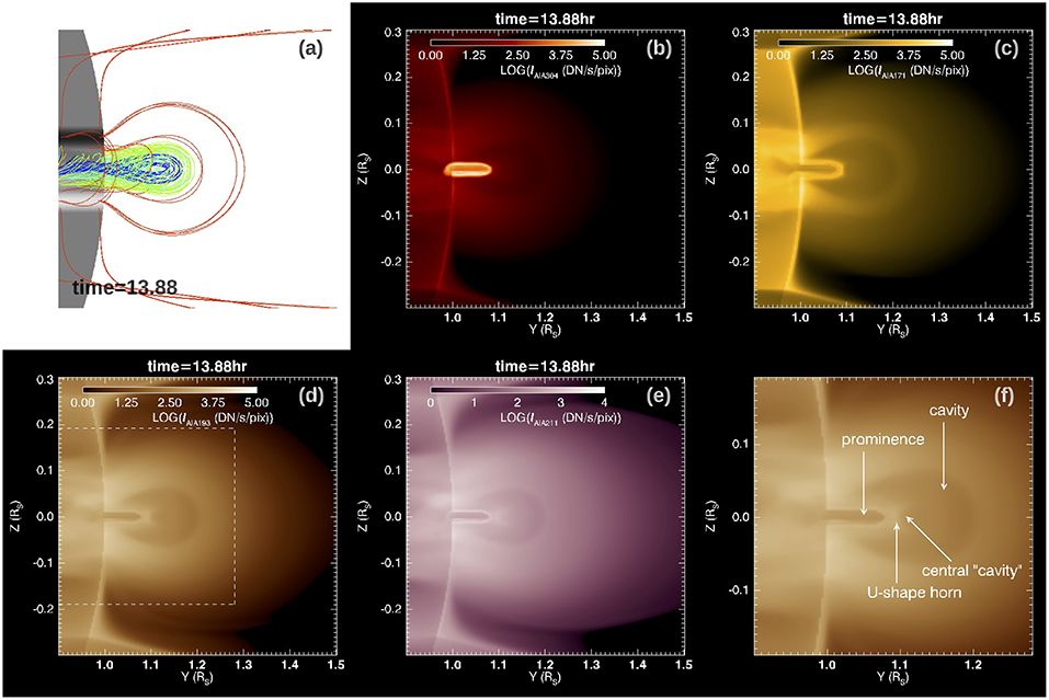
Figure 7. 3D field lines (a), and synthetic SDO/AIA EUV images in 304 Å (b), 171 Å (c), 193 Å (d), and 211 Å (e) channels, with the flux rope viewed along its axis above the limb, at time t = 13.88hr during the quasi-static phase. (f) shows the zoomed in view of the boxed area of (d) with the cavity substructures labeled.

FIGURE 8

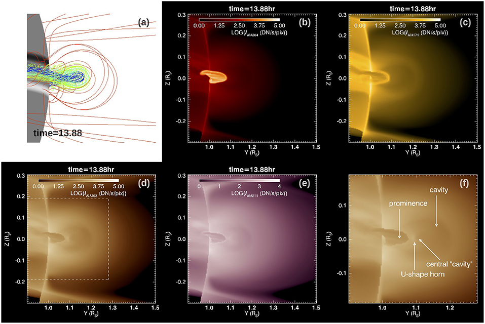
Figure 8. Same as Figure 7 but with the flux rope viewed slightly tilted by 5°.

Figure 9 shows a set of selected prominence-carrying field lines that contain prominence dips and one representative arcade dome field line in the high density dome, together with a vertical cross-section of density placed at different locations (for the different panels a–e) along the flux rope. The prominence condensation is outlined by the pink temperature iso-surface with T = 7.5 × 10⁴K. It can be seen in Figures 9a–e that as the density cross-section slides along the flux rope, the prominence carrying field lines intersect the cross-section in the low density cavity region, except at the prominence dips. In other words, we find that the prominence and the surrounding cavity are threaded by the prominence-carrying field lines, with the cavity corresponding to the density-depleted portions of the prominence-carrying field lines extending up from the prominence dips. As was shown in F18, the runaway radiative cooling of the prominence condensations in the dips causes a lowered pressure and draining of plasma toward the dips, establishing a more rarefied atmosphere along the dip-to-apex portions of the prominence carrying field lines compared to the surrounding dome field lines without dips. We find that the cavity boundary corresponds to a sharp transition from the dipped prominence carrying field lines inside the cavity to the arcade-like field lines without dips outside in the higher density dome. This is illustrated in an example shown in Figure 10. Two field lines are traced from two adjacent points on the two sides of the cavity boundary, and they show very different connectivity to the lower boundary, with the one from inside the cavity being a long twisting field line carrying two prominence dips and the other from just outside the cavity being a significantly shorter arcade-like field line with no dips (see Figure 10c). Because of the drastic difference in the connectivity and whether there are prominence condensations, the two field lines show very different thermodynamic properties at their two adjacent points near the cavity boundary, giving rise to the sharp appearance of the EUV cavity boundary. Note that the arcade-like field line in the dome region shows mixed types of foot points, with one foot point connecting to the pre-existing bipolar bands and the other foot point in the emerging flux rope foot points, suggesting that there have been continued reconnections between the flux rope and the pre-existing arcade field.

FIGURE 9

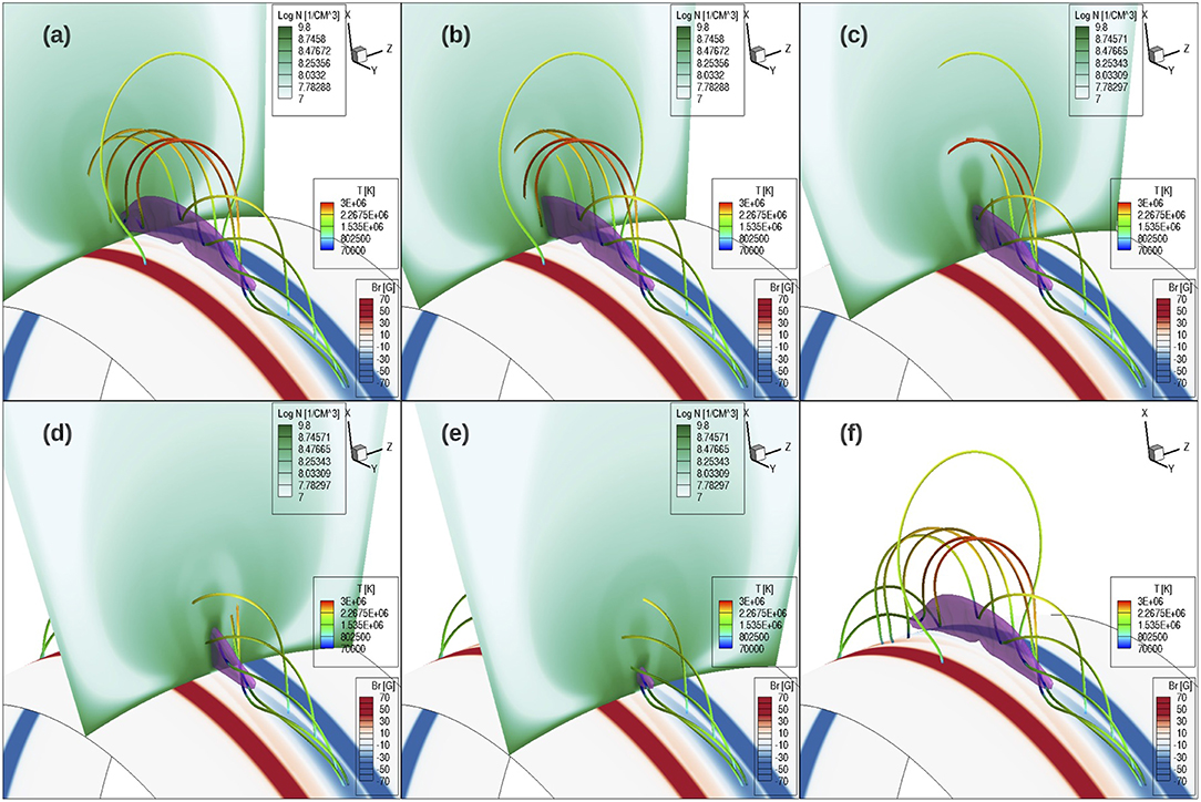
Figure 9. A set of prominence-carrying field lines containing prominence dips and one representative arcade dome field line, all colored with temperature, plotted with a cross-section of density placed at different locations along the flux rope for the different panels (a–e). (f) shows the same field lines without the density cross-section. A pink iso-surface of temperature at T = 7.5 × 10⁴K outlines the location of the prominence condensation. The lower boundary surface is colored with the normal magnetic field strength. All the images are at the time t = 13.88hr during the quasi-static stage.

FIGURE 10

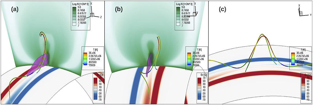
Figure 10. Two field lines traced from two adjacent points on the two sides of the cavity boundary in the density cross-section shown in (a,b) viewed from two different perspectives from opposite sides of the cross-section. The pink iso-surface of temperature at T = 7.5 × 10⁴ K outlines the prominence condensations. (c) shows the same field lines from a different view without the density cross-section and the iso-surface for the prominence. The lower boundary shows the normal magnetic field distribution B_r.

To examine the magnetic field that produces the substructure inside the EUV cavity, we have also traced field lines that thread through the region that contributes to the EUV emission of the prominence “horns.” Figure 11 shows a set of such field lines, together with a cross section showing the local emission intensity in EUV 193 Å channel (the integrand ${n_e}^2{f}_{193}(T)$ in Equation 2), with the cross-section placed at different locations along the flux rope for the different panels (a–e), and without showing the cross-section in panel (f). It can be seen that as the cross-section slides along the flux rope, the field lines intersect the central “U”-shaped region of enhanced EUV emission. As shown in Figure 11f, we find that these field lines that contribute to the prominence-horn emission are field lines containing relatively shallow dips, where the prominence condensations have evaporated to coronal temperatures (above 4 × 10⁵ K and with most parts of the field lines ranging between 8 × 10⁵ K and 2.2 × 10⁶ K) while the density is still relatively high compared to the surrounding cavity, and hence producing a favorable conditions for the enhanced EUV 193 Å channel emission. The cross-sections showing the EUV 193 Å channel emission intensity in Figures 11a–e also illustrate that enclosed inside the bright “U”-shaped prominence “horns” is another central region of reduced emission, corresponding to the central “cavity” seen in the synthetic EUV images (Figures 7d, 8d). Tracing field lines through this central “cavity" region, we find that it is threaded by long twisted field lines that contain no dips as shown in Figure 12. However as shown in the cross-sections in Figures 12a–c, this central “cavity” region is rather a relatively dense and hot central core. Its reduced EUV emission (compared to the horns and the outer dome region) is due to the high temperature (reaching about 2.5 MK) that is out of the peak of the EUV response function, instead of due to a low density as is the case for the outer cavity. We find that the outer boundary of the outer cavity has a hot rim of even higher temperature (see the cross section in Figure 12c) due to the heating resulting from continued reconnections between the dipped, twisted field lines that approach the cavity boundary and their neighboring arcade like field lines.

FIGURE 11

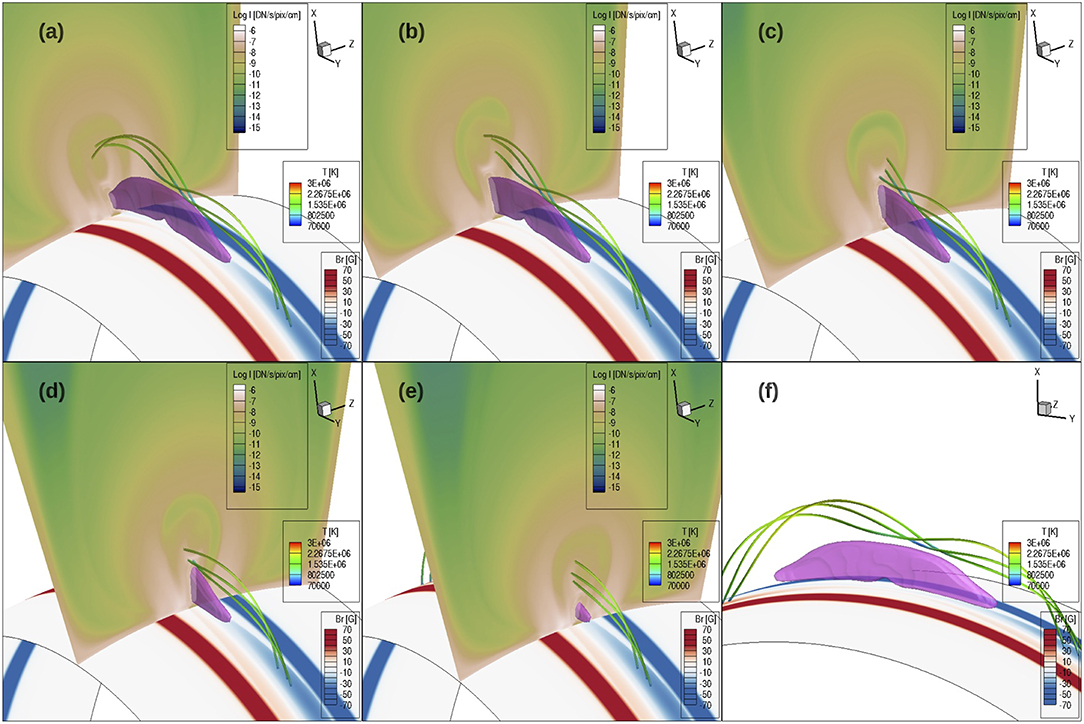
Figure 11. A set of field lines threading through the region that contributes to the EUV 193 Å channel emission that produces the horn-like structure inside the cavity, together with a cross-section showing the local emission intensity in EUV 193 Å channel (the integrand ${n_e}^2{f}_{193}(T)$ in Equation 2) placed at different locations along the flux rope for the different panels (a–e). (f) shows the same field lines without the cross-section and viewed from a different perspective. The field lines are colored in temperature. A pink iso-surface of temperature at T = 7.5 × 10⁴K outlines the location of the prominence condensation. The lower boundary surface is colored with the normal magnetic field strength. All the images are at the same time (t = 13.88hr) as those in Figure 9.

FIGURE 12

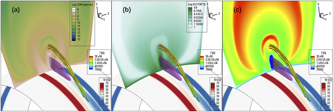
Figure 12. A set of field lines threading through the central EUV cavity enclosed in the prominence horns, together with a middle cross-section showing the distribution of EUV 193 Å channel emission intensity (a), density (b), and temperature (c). The field lines are colored in temperature and a pink iso-surface of temperature at T = 7.5 × 10⁴K outlining the location of the prominence condensation is also shown.

4. Conclusions

We have carried out MHD simulation of the quasi-static evolution and onset of eruption of a prominence-forming coronal flux rope under a coronal streamer, extending the previous work of F17 and F18. Previous simulations of the prominence-hosting coronal flux rope (the WS-L simulation in F17 and the PROM simulation in F18) have used the WS streamer solution in F17 for the pre-existing field, whose arcade field lines have a wide mean foot-point separation. This results in a corresponding potential field that declines slowly with height. Consequently the emerged flux rope and the prominence and cavity that form during the quasi-static stage reach large heights (larger than typically observed) before the onset of eruption. For the present simulation we have used a pre-existing streamer solution with a significantly narrower mean foot-point separation and stronger foot-point field strength for the arcade field lines. This results in a stronger field strength lower down and steeper decline of field strength with height for the corresponding potential field at the end of the flux emergence. We still drive the emergence of a similar long twisted flux rope into the corona as in the PROM case in F18. Similar to the PROM case, we find the formation of a prominence-cavity system during the quasi-static evolution, but with significantly lower heights for the prominence (reaching about 0.1R_s) and the cavity (extend to about 0.2R_s), in better agreement with the properties of the typically observed quiescent prominence-cavity systems. We also find the formation of cavity substructures, such as the prominence “horns” and central “voids” or “cavities” on top of the prominences, in qualitative agreement with the observed features (e.g., Gibson, 2015; Su et al., 2015).

We have examined the properties of the magnetic fields that comprise the different parts of the prominence-cavity system seen in the synthetic EUV images from our MHD model to understand the nature of the corresponding observed features. We find that the prominence and the outer cavity is composed of the long twisted field lines with dips that contain prominence condensations (Figure 9), where the cavity is threaded by the density depleted portions of the field lines extending up from the prominence dips. As was shown in F18, the formation of the prominence condensations due to runaway radiative cooling causes an overall lowered pressure in the dips and plasma draining down toward the dips such that a more rarefied atmosphere is established for the dip-to-apex portions of the field lines, compared to the surrounding arcade field lines in the denser helmet dome. We find that the boundary of the outer cavity corresponds to a sharp transition of field line connectivity, where neighboring field lines connect very differently to the lower boundary, with long twisted dipped field lines just inside the boundary and simple arcade-like field lines with no dips just outside (Figure 10). The very different thermodynamic properties of the two types of neighboring field lines give rise to the sharp appearance of the EUV cavity boundary. There are also continued magnetic reconnections at the boundary, causing a high temperature rim at the outer cavity boundary (see the temperature cross-section shown in Figure 12c) In regard to the cavity substructures, we find that the region of the central “U”-shaped prominence “horns” with relatively enhanced EUV emission inside the cavity are threaded by twisted field lines with relatively shallow dips, where the prominence condensations have evaporated to coronal temperatures while the density is still relatively high compared to the surrounding cavity (Figure 11). For the central “void” or “cavity” enclosed in the prominence “horns” on top of the prominence, we find that it corresponds to a central high temperature and high density core threaded by long twisted field lines with no dips (Figure 12). It appears as a central “void” with weakened EUV emission not because of a lower density, but because it is heated to a high temperature reaching about 2.5 MK that is outside of the peak of the AIA 193 Å channel (and also the AIA 211 Å channel) temperature response function. We find that the central high temperature core is growing over the course of the quasi-static phase. The prominence “horns” and growth of the central hot core result from a gradual transition of dipped prominence carrying field lines to un-dipped but still twisted field lines as they rise quasi-statically with the dips becoming shallower and the prominence condensations evaporating. The continued magnetic reconnection at the cavity boundary between the dipped twisted field lines and their neighboring arcade like field lines may be contributing to the quasi-static rise by removing the confining field. We defer to a follow-up paper to conduct a quasi-separatrix layer analysis (e.g., Pariat and Démoulin, 2012) to study the evolution of magnetic reconnection and how it contributes to the removal of the prominence mass and the rise of the flux rope during the quasi-static phase.

As was noted in F18, previous 3D MHD simulation of prominence formation in a stable flux rope by Xia et al. (2014), which includes the chromosphere as the lower boundary, has also found the formation of a prominence-cavity system with similar internal structures in synthetic EUV images. Their explanation of the structures obtained in their simulation is different from that found in our simulation. They found that the central dark cavity enclosed by the horns is threaded by two types of field lines: both the dipped twisted field lines and the arched twisted field lines with no dips, while the outer cavity is formed by arched twisted field lines with no dips. The prominence horns are due to the LOS emission from the prominence-corona transition regions of the prominence loaded dipped field lines. They found that during prominence-cavity formation, density depletion occurs not only on prominence-loaded field lines threading the cavity and prominence where in situ condensation happens (as is the case in our simulation), but also on prominence-free field lines due to mass drainage into the chromosphere. We do not find the latter type of field lines forming the cavity. Our outer main cavity is threaded by the density depleted portions of the prominence carrying dipped field lines, and the inner cavity is threaded by arched twisted field lines with no dips, which are not density depleted but appear dark in the EUV emission because they are heated to a high temperature (about 2.5 MK). In our simulations, the exclusion of the chromosphere and fixing the lower boundary at the transition region temperature do not allow modeling the change of the transition region height and hence limit the ability to model the condensation/drainage of plasma to the chromosphere with the cool chromosphere temperature region extending upwards. Furthermore our 3D simulations that model both the quasi-static phase and the eruption of prominence-carrying coronal flux ropes have much lower numerical resolution (1.9 Mm), compared to that achieved in Xia et al. (2014); Xia and Keppens (2016), which use adaptive grid refinement. As described in F17 we have modified the radiative loss function to suppress cooling for T ≤ 7 × 10⁴ K, so that the smallest pressure scale height (about 4.4 Mm) of the coolest plasma that forms does not go below two grid points given our simulation resolution. The low numerical resolution causes large numerical diffusion and viscosity that can impact significantly the heating and hydrodynamic evolution of the plasma. Because of the above limitations of our 3D simulations, the results of the thermodynamic properties of the resulting prominence-cavity system have large uncertainties, and need to be confirmed or revised by future higher resolution simulations that include the chromosphere in the lower boundary, which are our future work. The current simulation qualitatively illustrates the effect of the runaway radiative cooling of the prominence condensations in the dips of the twisted field lines that causes drainage of plasma of the upper portions of these field lines and creates a cavity with a relatively sharp boundary that corresponds to the transition from the dipped prominence carrying field lines to neighboring arcade-like field lines. It does not explain the formation of filament channels or coronal cavities in the absence of filament or prominence condensations.

We find that in the current simulation with a significantly narrower mean foot-point separation for the arcade field of the pre-existing streamer, the emerged flux rope begins to erupt at a significantly lower height compared to the PROM case shown in F18. This is due to the steeper decline with height of the corresponding potential field which allows the onset of the torus instability lower down. The eruption also produces a significantly faster CME compared to the PROM case, mainly due to the stronger field strength of the pre-eruption flux rope confined lower down. Although we find that the onset of eruption in the present case is consistent with the onset of the torus instability, due to the large total twist (about 1.76 winds of field line twist) in the emerged flux rope, both the erupting flux rope and the associated erupting prominence show significant rotational motion and develop a kinked morphology (Figures 2, 6).

Author Contributions

YF is the primary author of the paper who carried out the simulation, computed the synthetic images and directed the data analysis. TL carried out the 3D analysis of the simulation data that lead to the major findings of the paper and contributed to the writing of the paper.

Funding

NCAR is sponsored by the National Science Foundation. YF is supported in part by the Air Force Office of Scientific Research grant FA9550-15-1-0030 to NCAR. Visiting graduate student TL is supported by the scholarship from the Chinese Scholarship Council of the Ministry of Education of China, the National Natural Science Foundation of China grant NOS. 11473071 and 11790302 (11790300) and the Natural Science Foundation of Jiangsu Province (China) grant No. BK20141043.

Conflict of Interest Statement

The authors declare that the research was conducted in the absence of any commercial or financial relationships that could be construed as a potential conflict of interest.

Acknowledgments

We thank Dr. Jie Zhao for reading the paper and helpful comments on the paper.

References

Fan, Y. (2017). MHD simulations of the eruption of coronal flux ropes under coronal streamers. Astrophys. J. 844:26. doi: 10.3847/1538-4357/aa7a56

CrossRef Full Text | Google Scholar

Fan, Y. (2018). MHD simulation of prominence eruption. Astrophys. J. 862:54. doi: 10.3847/1538-4357/aaccee

CrossRef Full Text | Google Scholar

Gibson, S. (2015). “Coronal cavities: Observations and implications for the magnetic environment of prominences,” in Solar Prominences, eds. J. C. Vial and O. Engvold, Vol. 415, Astrophysics and Space Science Library (Cham: Springer), 323–353. doi: 10.1007/978-3-319-10416-4_13

CrossRef Full Text | Google Scholar

Hood, A. W., and Priest, E. R. (1981). Critical conditions for magnetic instabilities in force-free coronal loops. Geophys. Astrophys. Fluid Dynam. 17, 297–318. doi: 10.1080/03091928108243687

CrossRef Full Text | Google Scholar

Kliem, B., and Török, T. (2006). Torus Instability. Phys. Rev. Lett. 96:255002. doi: 10.1103/PhysRevLett.96.255002

PubMed Abstract | CrossRef Full Text | Google Scholar

Pariat, E., and Démoulin, P. (2012). Estimation of the squashing degree within a three-dimensional domain. Astron. Astrophys. 541:A78. doi: 10.1051/0004-6361/201118515

CrossRef Full Text | Google Scholar

Su, Y., van Ballegooijen, A., McCauley, P., Ji, H., Reeves, K. K., and DeLuca, E. E. (2015). Magnetic structure and dynamics of the erupting solar polar crown prominence on 2012 March 12. Astrophys. J. 807:144. doi: 10.1088/0004-637X/807/2/144

CrossRef Full Text | Google Scholar

Török, T., and Kliem, B. (2007). Numerical simulations of fast and slow coronal mass ejections. Astronom. Nachrich. 328, 743–746. doi: 10.1002/asna.200710795

CrossRef Full Text | Google Scholar

Webb, D. F., and Hundhausen, A. J. (1987). Activity associated with the solar origin of coronal mass ejections. Solar Phys. 108, 383–401. doi: 10.1007/BF00214170

CrossRef Full Text | Google Scholar

Xia, C., and Keppens, R. (2016). Formation and plasma circulation of solar prominences. Astrophys. J. 823:22. doi: 10.3847/0004-637X/823/1/22

CrossRef Full Text | Google Scholar

Xia, C., Keppens, R., Antolin, P., and Porth, O. (2014). Simulating the in situ condensation process of solar prominences. Astrophys. J. Lett. 792:L38. doi: 10.1088/2041-8205/792/2/L38

CrossRef Full Text | Google Scholar