How Rotating Solar Atmospheric Jets Become Kelvin–Helmholtz Unstable

1. Introduction

Solar jets are ubiquitous in the solar atmosphere and recent observations have revealed that they are related to small scale filament eruptions. They are continuously observed by the Extreme-ultraviolet Imaging Spectrometer (EIS) (Culhane et al., 2007) on board Hinode (Kosugi et al., 2007) satellite, Atmospheric Imaging Assembly (AIA) (Lemen et al., 2012), on board the Solar Dynamics Observatory (SDO) (Pesnell et al., 2012), as well as from the Interface Region Imaging Spectrograph (IRIS) (De Pontieu et al., 2014) alongside the Earth-based solar telescopes. The physical parameters of various kinds of solar jets have been reported in a series of articles (see for instance, Schmieder et al., 2013; Sterling et al., 2015; Panesar et al., 2016a; Chandra et al., 2017; Joshi et al., 2017, and references cited in). It was established that more of the solar jets possess rotational motion. Such tornado-like jets, termed macrospicules, were firstly detected in the transition region by Pike and Mason (1998) using observations by the Solar and Heliospheric Observatory (SOHO) (Domingo et al., 1995). Rotational motion in macrospicules was also explored by Kamio et al. (2010), Curdt and Tian (2011), Bennett and Erdélyi (2015), Kiss et al. (2017, 2018). Type II spicules, according to De Pontieu et al. (2012) and Martínez-Sykora et al. (2013), along with the coronal hole EUV jets (Liu et al., 2009; Nisticò et al., 2009, 2010; Shen et al., 2011; Chen et al., 2012; Hong et al., 2013; Young and Muglach, 2014a,b; Moore et al., 2015), and X-ray jets (Moore et al., 2013), can rotate, too. Rotating EUV jet emerging from a swirling flare (Zhang and Ji, 2014) or formed during a confined filament eruption (Filippov et al., 2015) confirm once again the circumstance that the rotational motion is a common property of many kinds of jets in the solar atmosphere.

The first scenario for the numerical modeling of hot X-ray jets was reported by Heyvaerts et al. (1997) and the basic idea was that a bipolar magnetic structure emerges into a unipolar pre-existing magnetic field and reconnects to form hot and fast jets that are emitted from the interface between the fields into contact. Later on, by examining many X-ray jets in Hinode/X-Ray Telescope coronal X-ray movies of the polar coronal holes, Moore et al. (2010) found that there is a dichotomy of polar X-ray jets, namely “standard” and “blowout” jets exist. Fang et al. (2014) studied the formation of rotating coronal jets through numerical simulation of the emergence of a twisted magnetic flux rope into a pre-existing open magnetic field. Another scenario for the nature of solar jets was suggested by Sterling et al. (2015), according to which the X-ray jets are due to flux cancellation and/or “mini-eruptions” rather than emergence. An alternative model for solar polar jets due to an explosive release of energy via reconnection was reported by Pariat et al. (2009). Using three-dimensional MHD simulations, the authors demonstrated that this mechanism does produce massive, high-speed jets. In subsequent two articles (Pariat et al., 2015, 2016), Pariat and co-authors, presented several parametric studies of a three-dimensional numerical MHD model for straight and helical solar jets. On the other side, Panesar et al. (2016b) have shown that the magnetic flux cancellation can trigger the solar quiet-region coronal jets and they claim that the coronal jets are driven by the eruption of a small-scale filament, called a “minifilament.” The small-scale chromospheric jets, like microspicules, were first numerically modeled by Murawski et al. (2011). Using the FLASH code, they solved the two-dimensional ideal MHD equations to model a macrospicule, whose physical parameters match those of a solar spicule observed. Another mechanism for the origin of macrospicules was proposed by Kayshap et al. (2013), who numerically modeled the triggering of a macrospicule and a jet.

It is natural to expect, that solar jets, being magnetically structured entities, should support the propagation of different type of MHD waves: fast and slow magnetoacoustic waves and torsional Alfvén waves. All these waves are usually considered as normal MHD modes traveling along the jet. Owing to the presence of a velocity shear near the jet–surrounding plasma interface, every jet can become unstable and the most universal instability which emerges is the Kelvin–Helmholtz (KH) one. The simplest configuration at which one can observe the KHI is the two semi-infinite incompressible magnetized plasmas flowing with different velocities provided that the thin velocity shear at the interface exceeds some critical value (Chandrasekhar, 1961). Recently, Cheremnykh et al. (2018a) theoretically established that shear plasma flows at the boundary of plasma media can generate eight MHD modes, of which only one can be unstable due to the development of the KHI. Ismayilli et al. (2018) investigated a shear instability of the KH type in a plasma with temperature anisotropy under the MHD approximation. The KHI of the magnetoacousic waves propagating in a steady asymmetric slab, and more specifically the effect of varying density ratios was explored by Barbulescu and Erdélyi (2018). A very good review on the KHI in the solar atmosphere, solar wind, and geomagnetosphere in the framework of ideal MHD the reader can find in Mishin and Tomozov, 2016.

In cylindrical geometry, being typical for the solar jets, the KHI exhibits itself as a vortex sheet running on the jet–environment boundary, which like in the flat geometry, is growing in time if the axial velocity of the jet in a frame of reference attached to the surrounding plasma exceeds a threshold value (Ryu et al., 2000). In its non-linear stage, the KHI trigger the wave turbulence which is considered as one of the main heating mechanisms of the solar corona (Cranmer et al, 2015). The development of the KHI in various cylindrical jet–environment configurations has been studied in photospheric jets (Zhelyazkov and Zaqarashvili, 2012), in solar spicules (Zhelyazkov, 2012; Ajabshirizadeh et al., 2015; Ebadi, 2016), in high-temperature and cool solar surges (Zhelyazkov et al., 2015a,b), in magnetic tubes of partially ionized compressible plasma (Soler et al., 2015), in EUV chromospheric jets (Zhelyazkov et al., 2016; Bogdanova et al., 2018), in soft X-ray jets (Vasheghani Farahani et al., 2009; Zhelyazkov et al., 2017), and in the twisted solar wind flows (Zaqarashvili et al., 2014). A review on KHI in the solar atmosphere, including some earlier studies, the reader can find in Zhelyazkov (2015).

The first modeling of the KHI in a rotating cylindrical magnetized plasma jet was done by Bondenson et al. (1987). Later on, Bodo et al. (1989, 1996) carried out a study of the stability of flowing cylindrical jet immersed in constant magnetic field B₀. The authors used the standard procedure for exploring the MHD wave propagation in cylindrical flows considering that all the perturbations of the plasma pressure p, fluid velocity v, and magnetic field B, are ∝exp[i(−ωt + kz + mθ)]. Here, ω is the angular wave frequency, k the propagating wavenumber, and m the azimuthal mode number. Using the basic equations of ideal magnetohydrodynamics, Bodo et al. (1989, 1996) derived a Bessel equation for the pressure perturbation and an expression for the radial component of the fluid velocity perturbation. The found solutions in both media (the jet and its environment) are merged at the perturbed tube boundary through the conditions for continuity of the total (thermal plus magnetic) pressure and the Lagrangian displacement. The latter is defined as the ratio of radial velocity perturbation component and the angular frequency in the corresponding medium. The obtained dispersion relation is used for examining the stability conditions of both axisymmetric, m = 0 (Bodo et al., 1989), and non-axisymmetric, |m| ⩾ 1 modes (Bodo et al., 1996). In a recent article, Bodo et al. (2016) performed a linear stability analysis of magnetized rotating cylindrical jet flows in the approximation of zero thermal pressure. They focused their analysis on the effect of rotation on the current driven mode and on the unstable modes introduced by rotation. In particular, they found that rotation has a stabilizing effect on the current driven mode only for rotation velocities of the order on the Alfvén speed. The more general case, when both the magnetic field and jet flow velocity are twisted, was studied by Zaqarashvili et al. (2015) and Cheremnykh et al. (2018b), whose dispersion equations for modes with m ⩾ 2, represented in different ways, yield practically identical results.

The main goal of this review article is to suggest a way of using the wave dispersion relation derived in Zaqarashvili et al. (2015) to study the possibility for the rising and development of KHI in rotating twisted solar jets. Among the enormous large number of observational studies of rotating jets with different origin or nature, we chose those which provide the magnitudes of axial and rotational speeds, jet width and height alongside the typical plasma parameters like electron number densities and electron temperature of the spinning structure and its environment. Thus, the targets of our exploration are: (i) the spinning coronal hole jet of 2010 August 21 (Chen et al., 2012); (ii) the rotating coronal hole jet of 2011 February 8 (Young and Muglach, 2014a), (iii) the twisted rotating jet emerging from a filament eruption on 2013 April 10–11 (Filippov et al., 2015), and (iv) the rotating macrospicule observed by Pike and Mason (1998) on 1997 March 8.

The paper is organized as follows: in the next section, we discuss the geometry of the problem, equilibrium magnetic field configuration and basic physical parameters of the explored jets. Section 3 is devoted to a short, concise, derivation of the wave dispersion relation. Section 4 deals with numerical results for each of the four jets and contain the available observational data. In the last section 5, we summarize the main findings in our research and outlook the further improvement of the used modeling.

2. The Geometry, Magnetic Field, and Physical Parameters in a Jet Model

We model whichever jet as an axisymmetric cylindrical magnetic flux tube with radius a and electron number density n_i (or equivalently, homogeneous plasma density ρ_i) moving with velocity U. We consider that the jet environment is a rest plasma with homogeneous density ρ_e immersed in a homogeneous background magnetic field B_e. This field, in cylindrical coordinates (r, ϕ, z), possesses only an axial component, i.e., B_e = (0, 0, B_e) (Note that the label “i” is abbreviation for interior, and the label “e” denotes exterior). The magnetic field inside the tube, B_i, and the jet velocity, U, we assume, are uniformly twisted and are given by the vectors

$\begin{array}{ll}{B}_{\text{i}}=(0,B_{\text{i}\varphi }(r),B_{\text{i}z})\text{\hspace{1em} and\hspace{1em} }U=(0,U_{\varphi }(r),U_z),& (1)\end{array}$

respectively. We note, that B_iz and U_z, are constant. Concerning the azimuthal magnetic and flow velocity components, we suppose that they are linear functions of the radial position r and evaluated at r = a they correspondingly are equal to B_iϕ(a) ≡ B_ϕ = Aa and U_ϕ = Ωa, where A and Ω are constants. Here, Ω is the jet angular speed, deduced from the observations. Hence, in equilibrium, the rigidly rotating plasma column, that models the jet, must satisfy the following force-balance equation (see, e.g., Chandrasekhar, 1961; Goossens et al., 1992)

$\begin{array}{ll}\frac{\text{d}}{\text{d}r}\left(p_{\text{i}}+\frac{B_{\text{i}}^2}{2\mu }\right)=\frac{{\rho }_{\text{i}}{U}_{\varphi }^2}{r}-\frac{B_{\text{i}\varphi }^2}{\mu r},& (2)\end{array}$

where μ is the plasma permeability and $p_{\text{t}}=p_{\text{i}}+B_{\text{i}}^2/2\mu$ with $B_{\text{i}}^2=B_{\text{i}\varphi }^2(r)+B_{\text{i}z}^2$ is the total (thermal plus magnetic) pressure. According to Equation (2), the radial gradient of the total pressure should balance the centrifugal force and the force owing to the magnetic tension. After integrating Equation (2) from 0 to a, taking into account the linear dependence of U_ϕ and B_iϕ on r, we obtain that

$p_{\text{t}}(a)=p_{\text{t}}(0)+\frac{1}{2}{\rho }_{\text{i}}{U}_{\varphi }^2(a)-\frac{B_{\text{i}\varphi }^2(a)}{2\mu },$

where $p_{\text{t}}(0)=p_1(0)+B_{\text{i}z}^2/2\mu$. Integrating Equation (2) from 0 to any r one can find the radial profile of p_t inside the tube. Such an expression of p_t(r), obtained, however, from an integration of the momentum equation for the equilibrium variables, have been obtained in Zhelyazkov et al. (2018)—see Equation (2) there. It is clear from a physical point of view that the internal total pressure (evaluated at r = a) must be balanced by the total pressure of the surrounding plasma which implies that

$p_1(0)+\frac{B_{\text{i}z}^2}{2\mu }-\frac{B_{\text{i}\varphi }^2(a)}{2\mu }+\frac{1}{2}{\rho }_{\text{i}}{U}_{\varphi }^2(a)=p_{\text{e}}+\frac{B_{\text{e}}^2}{2\mu }.$

This equation can be presented in the form

$\begin{array}{ll}{p}_1(0)+\frac{1}{2}{\rho }_{\text{i}}{U}_{\varphi }^2(a)+\frac{B_{\text{i}z}^2}{2\mu }(1-{\epsilon }_1^2)=p_{\text{e}}+\frac{B_{\text{e}}^2}{2\mu },& (3)\end{array}$

where p₁(0) is the thermal pressure at the magnetic tube axis, and p_e denotes the thermal pressure in the environment. In the pressure balance Equation (3), the number ε₁ ≡ B_ϕ/B_iz = Aa/B_iz represents the magnetic field twist parameter. Similarly, we define ε₂ ≡ U_ϕ/U_z as a characteristics of the jet velocity twist. We would like to underline that the choice of plasma and environment parameters must be such that the total pressure balance Equation (3) is satisfied. In our case, the value of ε₂ is fixed by observationally measured rotational and axial velocities while the magnetic field twist, ε₁, has to be specified when using Equation (3). We have to note that Equation (3) is a corrected version of the pressure balance equation used in Zhelyazkov et al. (2018) and Zhelyazkov and Chandra (2018).

From measurements of n and T for similar coronal hole EUV jets (Nisticò et al., 2009, 2010), we take n inside the jet to be $n_{\text{i}}=1.0\times 10^9$ cm⁻³, and assume that the electron temperature is T_i = 1.6 MK. The same quantities in the environment are, respectively, $n_{\text{e}}=0.9\times 10^9$ cm⁻³ and T_e = 1.0 MK. Note that the electron number density of the blowout jet observed by Young and Muglach (2014a) is in one order lower. The same applies for its environment. We consider that the background magnetic field for both hole coronal jets is B_e = 3 G. The values of n and T of the rotating jet emerging from a filament eruption, observed by Filippov et al. (2015), were evaluated by us and they are $n_{\text{i}}=4.65\times 10^9$ cm⁻³ and T_i = 2.0 MK, respectively. From the same data set, we have obtained $n_{\text{e}}=4.02\times 10^9$ cm⁻³ and T_e = 2.14 MK. The background magnetic field, B_e, with which the pressure balance Equation (3) is satisfied, is equal to 6 G. For the rotating macrospicule we assume that $n_{\text{i}}=1.0\times 10^{10}$ cm⁻³ and $n_{\text{e}}=1.0\times 10^9$ cm⁻³ to have at least one order denser jet with respect to the surrounding plasma. Our choice for macrospicule temperature is $T_{\text{i}}=5.0\times 10^5$ K, while that of its environment is supposed to be $T_{\text{e}}=1.0\times 10^6$ K. The external magnetic field, B_e, was taken as 5 G. All aforementioned physical parameters of the jets are summarized in Table 1. The plasma beta was calculated using $(6/5)c_{\text{s}}^2/v_{\text{A}}^2$, where $c_{\text{s}}={(\gamma k_{\text{B}}T/m_{\text{ion}})}^{1/2}$ is the sound speed (in which γ = 5/3, k_B is the Boltzmann's constant, T the electron temperature, and m_ion the ion or proton mass), and $v_{\text{A}}=B/{(\mu n_{\text{ion}}{m}_{\text{ion}})}^{1/2}$ is the Alfvén speed, in which expression B is the full magnetic field $={(B_{\varphi }^2+B_z^2)}^{1/2}$, and n_ion is the ion or proton number density.

TABLE 1

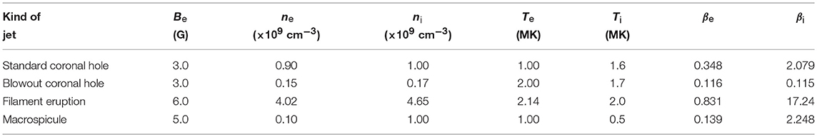
Table 1. Jets physical parameters derived from observational data.

3. Wave Dispersion Relation

A dispersion relation for the propagation of high-mode (m ⩾ 2) MHD waves in a magnetized axially moving and rotating twisted jet was derived by Zaqarashvili et al. (2015) and Cheremnykh et al. (2018b). That equation was obtained, however, under the assumption that both media (the jet and its environment) are incompressible plasmas. As seen from the last column in Table 1, plasma beta is greater than 1 in the first, third, and fourth jets which implies that the plasma of each of the aforementioned jets can be considered as a nearly incompressible fluid (Zank and Matthaeus, 1993). It is seen from the same table that the plasma beta of the second jet is less than one as is in each of the jet environments and that is why it is reasonable to treat them as cool media. Thus, the wave dispersion relation, derived, for instance, in Zaqarashvili et al. (2015), has to be modified. In fact, we need two modified versions: one for the incompressible jet–cool environment configuration, and other for the cool jet–cool environment configuration. We are not going to present in details the derivation of the modified dispersion equations on the basis of the governing MHD equations, but will only sketch the essential steps in that procedure. The main philosophy in deriving the wave dispersion equation is to find solutions for the total pressure perturbation, p_tot, and for the radial component, ξ_r of the Lagrangian displacement, ξ, and merge them at the tube perturbed boundary through the boundary conditions for their (p_tot and ξ_r) continuity (Chandrasekhar, 1961). In the case of the first configuration, we start with the linearized ideal MHD equations, governing the incompressible dynamics of the perturbations in the spinning jet

$\begin{array}{ll}\frac{\partial }{\partial t}v+(U·\nabla )v+(v·\nabla )U=-\frac{\nabla p_{\text{tot}}}{{\rho }_{\text{i}}}+\frac{(B_{\text{i}}·\nabla )b}{{\rho }_{\text{i}}\mu }+\frac{(b·\nabla )B_{\text{i}}}{{\rho }_{\text{i}}\mu },& (4)\end{array}$

$\begin{array}{ll}\frac{\partial }{\partial t}b-\nabla \times (v\times B_{\text{i}})-\nabla \times (U\times b)=0,& (5)\end{array}$

$\begin{array}{ll}\nabla ·v=0,& (6)\end{array}$

$\begin{array}{ll}\nabla ·b=0,& (7)\end{array}$

where v = (v_r, v_ϕ, v_z) and B = (b_r, b_ϕ, b_z) are the perturbations of fluid velocity and magnetic field, respectively, and p_tot is the perturbation of the total pressure, $p_{\text{t}}=p_{\text{i}}+B_{\text{i}}^2/2\mu$. The Lagrangian displacement, ξ, can be found from the fluid velocity perturbation, v, using the relation (Chandrasekhar, 1961)

$\begin{array}{ll}v=\frac{\partial \xi }{\partial t}+(U·\nabla )\xi -(\xi ·\nabla )U.& (8)\end{array}$

Further on, assuming that all perturbations are ∝exp[i(−ωt + mϕ + k_zz)] and considering that the rotation and the magnetic field twists in the jet are uniform, that is,

$\begin{array}{ll}{U}_{\varphi }(r)=\Omega r\text{\hspace{1em} and\hspace{1em} }{B}_{\text{i}\varphi }(r)=Ar,& (9)\end{array}$

where Ω and A are constants, from the above set of Equations (4–8), we obtain the following dispersion equation of the MHD wave with mode number m (for details see Zaqarashvili et al., 2015):

$\begin{array}{l}\frac{({\sigma }^2-{\omega }_{\text{Ai}}^2)F_m({\kappa }_{\text{i}}a)-2m(\sigma \Omega +A{\omega }_{\text{Ai}}/\sqrt{\mu {\rho }_{\text{i}}})}{{\rho }_{\text{i}}{({\sigma }^2-{\omega }_{\text{Ai}}^2)}^2-4{\rho }_{\text{i}}{(\sigma \Omega +A{\omega }_{\text{Ai}}/\sqrt{\mu {\rho }_{\text{i}}})}^2}\\ =\frac{P_m({\kappa }_{\text{e}}a)}{{\rho }_{\text{e}}({\omega }^2-{\omega }_{\text{Ae}}^2)-({\rho }_{\text{i}}{\Omega }^2-A^2/\mu )P_m({\kappa }_{\text{e}}a)},& (10)\end{array}$

where

$F_m({\kappa }_{\text{i}}a)=\frac{{\kappa }_{\text{i}}a{I}_m^{\prime }({\kappa }_{\text{i}}a)}{I_m({\kappa }_{\text{i}}a)}\text{\hspace{1em}and\hspace{1em}}{P}_m({\kappa }_{\text{e}}a)=\frac{{\kappa }_{\text{e}}a{K}_m^{\prime }({\kappa }_{\text{e}}a)}{K_m({\kappa }_{\text{e}}a)}.$

In above expressions, the prime means differentiation of the Bessel functions with respect to their arguments,

$\begin{array}{l}{\kappa }_{\text{i}}^2=k_z^2\left[1-4{\left(\frac{\sigma \Omega +A{\omega }_{\text{Ai}}/\sqrt{\mu {\rho }_{\text{i}}}}{{\sigma }^2-{\omega }_{\text{Ai}}^2}\right)}^2\right]\text{\hspace{1em}and}\\ {\kappa }_{\text{e}}^2=k_z^2\left[1-{(\omega /{\omega }_{\text{Ae}})}^2\right]\end{array}$

are the squared wave amplitude attenuation coefficients in the jet and its environment, in which

${\omega }_{\text{Ai}}=\left(\frac{m}{r}{B}_{\text{i}\varphi }+k_z{B}_{\text{i}z}\right)/\sqrt{\mu {\rho }_{\text{i}}}\text{\hspace{1em}and\hspace{1em}}{\omega }_{\text{Ae}}=k_z{B}_{\text{e}}/\sqrt{\mu {\rho }_{\text{e}}}$

are the local Alfvén frequencies in both media, and

$\sigma =\omega -\frac{m}{r}{U}_{\varphi }-k_z{U}_z$

is the Doppler-shifted angular wave frequency in the jet. We note that in the case of incompressible coronal plasma (Zaqarashvili et al., 2015), κ_e = k_z, because at an incompressible environment the argument of the modified Bessel function of second kind, K_m, and its derivative, $K_m^{\prime }$, is k_za.

The basic MHD equations for an ideal cool plasma are, generally, the same as the set of Equations (4–8) with Equation (6) replaced by the continuity equation

$\begin{array}{l}\frac{\partial {\rho }_1}{\partial t}=-\nabla ·({\rho }_0{v}_1+{\rho }_{1}U)=0.\end{array}$

Recall that for cold plasmas the total pressure reduces to the magnetic pressure only, that is $p_{\text{t}}=B_1^2/2\mu$, the z component of the velocity perturbation is zero, i.e., v₁ = (v_1r, v_1ϕ, 0), while B₁ = (B_1r, B_1ϕ, B_1z). The above equation, which defines the density perturbation, is not used in the derivation of the wave dispersion relation because we are studying the propagation and stability of Alfvén-wave-like perturbations of the fluid velocity and magnetic field. Following the standard scenario for deriving the MHD wave dispersion relation (Zhelyazkov and Chandra, 2018), we finally arrive at:

$\begin{array}{l}\frac{({\sigma }^2-{\omega }_{\text{Ai}}^2)F_m({\kappa }_{\text{i}}^{\text{c}}a)-2m(\sigma \Omega +A{\omega }_{\text{Ai}}/\sqrt{\mu {\rho }_{\text{i}}})}{{\rho }_{\text{i}}{({\sigma }^2-{\omega }_{\text{Ai}}^2)}^2-4{\rho }_{\text{i}}{(\sigma \Omega +A{\omega }_{\text{Ai}}/\sqrt{\mu {\rho }_{\text{i}}})}^2}\\ =\frac{P_m({\kappa }_{\text{e}}^{\text{c}}a)}{{\rho }_{\text{e}}({\omega }^2-{\omega }_{\text{Ae}}^2)-({\rho }_{\text{i}}{\Omega }^2-A^2/\mu )P_m({\kappa }_{\text{e}}^{\text{c}}a)},& (11)\end{array}$

where

$F_m({\kappa }_{\text{i}}^{\text{c}}a)=\frac{{\kappa }_{\text{i}}^{\text{c}}a{I}_m^{\prime }({\kappa }_{\text{i}}^{\text{c}}a)}{I_m({\kappa }_{\text{i}}^{\text{c}}a)}\text{\hspace{1em}and\hspace{1em}}{P}_m({\kappa }_{\text{e}}^{\text{c}}a)=\frac{{\kappa }_{\text{e}}^{\text{c}}a{K}_m^{\prime }({\kappa }_{\text{e}}^{\text{c}}a)}{K_m({\kappa }_{\text{e}}^{\text{c}}a)}.$

Here, the wave attenuation coefficient in the internal medium has the form

${\kappa }_{\text{i}}^{\text{c}}=k_z{\left\{1-4{\left(\frac{\sigma \Omega +A{\omega }_{\text{Ai}}/\sqrt{\mu {\rho }_{\text{i}}}}{{\sigma }^2-{\omega }_{\text{Ai}}^2}\right)}^2\right\}}^{1/2}{\left(1-\frac{{\sigma }^2}{{\omega }_{\text{Ai}}^2}\right)}^{1/2},$

while that in the environment, with Ω = 0 and A = 0, is given by

${\kappa }_{\text{e}}^{\text{c}}=k_z{\left(1-\frac{{\omega }^2}{{\omega }_{\text{Ae}}^2}\right)}^{1/2}.$

Note that (i) both dispersion relations, (10) and (11), have similar forms—the difference is in the expressions for the wave attenuation coefficient inside the jet, namely ${\kappa }_{\text{i}}^{\text{c}}={\kappa }_{\text{i}}{\left[1-{\sigma }^2/{\omega }_{\text{Ai}}^2\right]}^{1/2}$; and (ii) the wave attenuation coefficients in the environments are not surprisingly the same, that is, ${\kappa }_{\text{e}}^{\text{c}}={\kappa }_{\text{e}}\equiv {\left[1-{\omega }^2/{\omega }_{\text{Ae}}^2\right]}^{1/2}$.

4. Numerical Solutions, Wave Dispersion, and Growth Rate Diagrams

In studying at which conditions the high (m ⩾ 2) MHD modes in a jet–coronal plasma system become unstable, that is, all the perturbations to grow exponentially in time, we have to consider the wave angular frequency, ω, as a complex quantity: ω ≡ Re(ω) + iIm(ω) in contrast to the wave mode number, m, and propagating wavenumber, k_z, which are real quantities. The Re(ω) is responsible for the wave dispersion while the Im(ω) yields the wave growth rate. In the numerical task for finding the complex solutions to the wave dispersion relation (10) or (11), it is convenient to normalize all velocities with respect to the Alfvén speed inside the jet, defined as $v_{\text{Ai}}=B_{\text{i}z}/\sqrt{\mu {\rho }_{\text{i}}}$, and the lengths with respect to a. Thus, we have to search the real and imaginary parts of the non-dimensional wave phase velocity, v_ph = ω/k_z, that is, Re(v_ph/v_Ai) and Im(v_ph/v_Ai) as functions of the normalized wavenumber k_za. The normalization of the other quantities like the local Alfvén and Doppler-shifted frequencies alongside the Alfvén speed in the environment, $v_{\text{Ae}}=B_{\text{e}}/\sqrt{\mu {\rho }_{\text{e}}}$, requires the usage of both twist parameters, ε₁ and ε₂, and also of the magnetic fields ratio, b = B_e/B_iz. The non-dimensional form of the jet axial velocity, U_z, is given by the Alfvén Mach number M_A = U_z/v_Ai. Another important non-dimensional parameter is the density contrast between the jet and its surrounding medium, η = ρ_e/ρ_i. Hence, the input parameters in the numerical task of finding the solutions to the transcendental Equation (10) or (11) (in complex variables) are: m, η, ε₁, ε₂, b, and M_A. Zaqarashvili et al. (2015) have established that KHI in an untwisted (A = 0) rotating flux tube with negligible longitudinal velocity can occur if

$\begin{array}{ll}\frac{a^2{\Omega }^2}{v_{\text{Ai}}^2}>\frac{1+\eta }{1+\left|m\right|\eta }\frac{{(k_{z}a)}^2}{\left|m\right|-1}(1+b^2).& (12)\end{array}$

This inequality says that each MHD wave with mode number m ⩾ 2, propagating in a rotating jet can become unstable. This instability condition can be used also in the cases of slightly twisted spinning jets, provided that the magnetic field twist parameter, ε₁, is a number lying in the range of 0.001–0.005, simply because the numerical solutions, for example, to Equation (10) show that practically there is no difference between the instability ranges at ε₁ = 0, and at 0.001 or 0.005. An important step in our study is the supposition that the deduced from observations jet axial velocity, U_z, is the threshold speed for the KHI occurrence. Then, for fixed values of m, η, U_ϕ = Ωa, v_Ai, and b, the inequality (12) can be rearranged to define the upper limit of the instability range on the k_za-axis

$\begin{array}{ll}{(k_{z}a)}_{\text{rhs}}<{\left\{{\left(\frac{U_{\varphi }}{v_{\text{Ai}}}\right)}^2\frac{1+\left|m\right|\eta }{1+\eta }\frac{\left|m\right|-1}{1+b^2}\right\}}^{1/2}.& (13)\end{array}$

According to the above inequality, the KHI can occur for nondimensional wavenumbers k_za less than (k_za)_rhs. On the other hand, one can talk for instability if the unstable wavelength, λ_KH = 2π/k_z, is shorter than the height of the jet, H, which means that the lower limit of the instability region is given by:

$\begin{array}{ll}{(k_{z}a)}_{\text{lhs}}>\frac{\pi \Delta \ell }{H},& (14)\end{array}$

where Δℓ is the jet width. Hence, the instability range in the k_za-space is (k_za)_lhs < k_za < (k_za)_rhs. Note that the lower limit, (k_za)_lhs, is fixed by the width and height of the jet, while the upper limit, (k_za)_rhs, depends on several jet–environment parameters. At fixed U_ϕ, v_Ai, η, and b, the (k_za)_rhs is determined by the MHD wave mode number, |m|. As seen from inequality (13), with increasing the m, that limit shifts to the right, that is, the instability range becomes wider. The numerical solutions to the wave dispersion relation (10) confirm this and for given m one can obtain a series of unstable wavelengths, λ_KH = πΔℓ/k_za, as the shortest one takes place at k_za ≈ (k_za)_rhs. For relatively small mode numbers, when even the shortest unstable wavelengths turn out to be a few tens megameters, that could hardly be associated with the observed KH ones. As observations show, the KHI vortex-like structures running at the boundary of the jet, have the size of the width or radius of the flux tube (see, for instance, Figure 1 in Zhelyazkov et al., 2018). Therefore, we have to look for such an m, whose instability range would accommodate the expected unstable wavelength presented by its nondimensional wavenumber, k_za = πΔℓ/λ_KH. An estimation of the required mode number for an ε₁ = 0.005-rotating flux tube can be obtained by presenting the instability criterion (12) in the form

$\begin{array}{ll}\eta |m{|}^2+(1-\eta )|m|-1-\frac{{(k_{z}a)}^2(1+\eta )(1+b^2)}{{(U_{\varphi }/v_{\text{Ai}})}^2}>0.& (15)\end{array}$

We will use this inequality for obtaining the optimal m for each of the studied jets by specifying the value of that k_za (along with the other aforementioned input parameters) which corresponds to the expected unstable wavelength λ_KH.

FIGURE 1

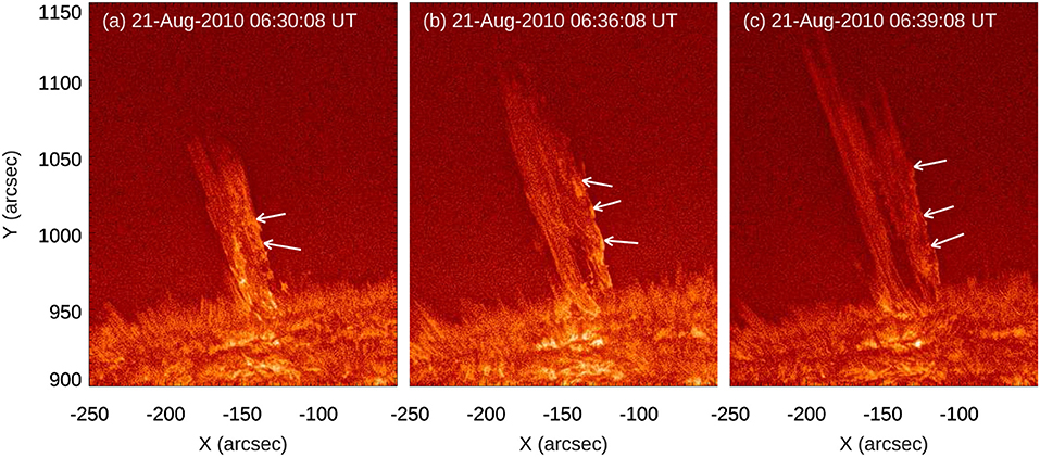
Figure 1. AIA 304 Å images showing the detailed evolution of the jet observed on 2010 August 21. The small moving blobs on the right side boundary of the jet as indicated by white arrows, could be produced by a KHI.

4.1. Kelvin–Helmholtz Instability in a Standard Polar Coronal Hole Jet

Chen et al. (2012) observationally studied the jet event of 2010 August 21, which occurred in the coronal hole region, close to the north pole of the Sun. Figure 1 presents the jet's evolution in AIA 304 Å. The jet started around 06:07 UT, reached its maximum height around 06:40 UT. During the evolution of the jet between 06:32 and 06:38 UT, small scale moving blobs appeared on the right boundary. We interpret these blobs, shown by arrows in Figure 1, as evidence of KHI. By tracking six identified moving features in the jet, Chen et al. (2012) found that the plasma moved at an approximately constant speed along the jet's axis. Inferred from linear and trigonometric fittings to the axial and transverse heights of the six tracks, the authors have found that the mean values of the axial velocity, U_z, transfer/rotational velocity, U_ϕ, angular speed, Ω, rotation period, T, and rotation radius, a, are 114 km s⁻¹, 136 km s⁻¹, 0.81°s⁻¹ (or 14.1 × 10⁻³ rad s⁻¹), 452 s, and 9.8 × 10³ km, respectively. The height of the jet is evaluated as H = 179 Mm.

It seems reasonable the shortest unstable wavelength, λ_KH, to be equal to 10 Mm (approximately half of the jet width, Δℓ = 19.6 Mm), which implies that its position on the k_za one-dimensional space is k_za = 6.158. The input parameters, necessary to find out that MHD wave mode number, whose instability range will contain the nondimensional wavenumber of 6.158, using inequality (15), are accordingly (see Table 1) η = 0.9, b = 1.834, v_Ai = 112.75 km s⁻¹, and U_ϕ = 136 km s⁻¹ (We note, that the values of b and v_Ai were obtained with the help of Equation (3) assuming that the magnetic field twist is ε₁ = 0.005). With these entry data, from inequality (15) one obtains that |m| > 15 should provide the required instability region or window. The numerical solutions to Equation (10) show that this value of m is overestimated—an m = 11 turns out to be perfect for the case. The discrepancy between the predicted and computed value of |m| is not surprising because inequality (15) yields only an indicative value. The input parameters for finding the solutions to the dispersion Equation (10) are as follows: m = 11, η = 0.9, ε₁ = 0.005, ε₂ = 1.2, b = 1.834, and M_A = 1.01 (= 114/112.75). The results of computations are graphically presented in Figure 2. From that figure, one can obtain the normalized wave phase velocity, Re(v_ph/v_Ai), and the normalized growth rate, Im(v_ph/v_Ai), of the unstable λ_KH = 10 Mm wave, both read at the purple cross points. From the same plot, one can find the instability characteristics at another wavelength, precisely λ_KH = 12 Mm, whose position on the k_za-axis is fixed at k_za = 5.131. The values of nondimensional wave phase velocity and growth rate can be read from the green cross points. The KHI wave growth rate, γ_KH, growth time, τ_KH = 2π/γ_KH, and wave velocity, v_ph, in absolute units, estimated from the plots in Figure 2, for the two wavelengths, are

$\begin{array}{l}{\gamma }_{\text{KH}}\cong 23.09\times 10^{-3}{\text{s}}^{-1},{\tau }_{\text{KH}}\cong 4.5\text{ min},v_{\text{ph}}\cong 178\text{ km }{\text{s}}^{-1},\\ \text{for }{\lambda }_{\text{KH}}=10\text{ Mm},\end{array}$

and

$\begin{array}{l}{\gamma }_{\text{KH}}\cong 50.65\times 10^{-3}{\text{s}}^{-1},{\tau }_{\text{KH}}\cong 2.1\text{ min},v_{\text{ph}}\cong 202\text{ km }{\text{s}}^{-1},\\ \text{for }{\lambda }_{\text{KH}}=12\text{ Mm}.\end{array}$

Let us recall that the value of the Alfvén speed used in the normalization is v_Ai = 112.75 km s⁻¹. We see that the two wave phase velocities are slightly super-Alfvénic and when moving along the k_za-axis to the left, the normalized wave velocity becomes higher. If we fix a k_za-position near the lower limit of the unstable region, (k_za)_lhs = 0.344, say, at k_za = 0.513, which means λ_KH = 120 Mm, the KHI characteristics obtained from the numerical solutions to Equation (10) are τ_KH = 1.4 min and v_ph = 1473 km s⁻¹, respectively. As we have discussed in Zhelyazkov et al. (2018), “the KHI growth time could be estimated from the temporal evolution of the blobs in their initial stage and it was found to be about 2–4 min,” so the instability developing times of 2.1 and 4.5 min obtained from our plots are in good agreement with the observations.

FIGURE 2

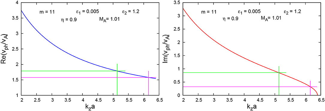
Figure 2. (Left) Dispersion curve of the m = 11 MHD mode propagating along a twisted incompressible coronal hole jet at η = 0.9, b = 1.834, M_A = 1.01, ε₁ = 0.005, and ε₂ = 1.2. (Right) Normalized growth rate curve of the m = 11 MHD mode computed at the same input parameters as in the left panel. The crosses of purple and green lines yield the normalized values of the wave phase velocity and the wave growth rate at the two unstable wavelengths of 10 and 12 Mm, respectively.

A specific property of the instability k_za-ranges is that for a fixed mode number, m, their widths depend upon ε₁ and with increasing the value of ε₁, the instability window becomes narrower and at some critical ε₁ its width equals zero. In our case that happens with ${\epsilon }_1^{\text{cr}}=0.653577$ at (k_za)_lhs = 0.344. In Figure 3, curves of dimensionless v_ph and γ_KH have been plotted for several ε₁ values. Note that each larger value of ε₁ implies an increase in B_iϕ. But that increase in B_iϕ requires an increase in B_iz too, in order the total pressure balance Equation (3) to be satisfied under the condition that the hydrodynamic pressure term and the environment total pressure are fixed. The increase in B_iz (and in the full magnetic field B_i) implies a decrease both in the magnetic field ratio, b, and in the Alfvén Mach number, M_A. Thus, gradually increasing the magnetic field twist ε₁ from 0.005 to 0.653577, we get a series of dispersion and growth rate curves with progressively diminishing parameters b and M_A. The red growth rate curve in the right panel of Figure 3 has been obtained for ${\epsilon }_1^{\text{cr}}=0.653577$ with M_A = 0.7652 and it visually fixes the lower limit of all other instability windows. The azimuthal magnetic field $B_{\text{i}\varphi }^{\text{cr}}$ that stops the KHI, computed at B_i = 2.58 G, is equal to 1.4 G.

FIGURE 3

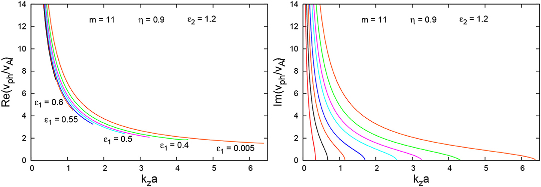
Figure 3. (Left) Dispersion curves of the unstable m = 11 MHD mode propagating along a twisted incompressible jet in a coronal hole at η = 0.9, ε₂ = 1.2, and the following values of ε₁ (from right to left): 0.005, 0.4, 0.5, 0.55, 0.6, 0.625, 0.645, and 0.653577 (red curve in the right plot). Alfvén Mach numbers for these curves are, respectively 1.01, 0.93, 0.88, 0.84, 0.81, 0.79, 0.77, and 0.7653. (Right) Growth rates of the unstable m = 11 mode for the same input parameters. The azimuthal magnetic field that corresponds to ${\epsilon }_1^{\text{cr}}=0.653577$ (the instability window with zero width) and stops the KHI onset is equal to 1.4 G.

4.2. Kelvin–Helmholtz Instability in a Blowout Polar Coronal Hole Jet

Young and Muglach (2014a) observed a small blowout jet at the boundary of the south polar coronal hole on 2011 February 8 at around 21:00 UT. The evolution of jet observed by the AIA is displayed in Figure 4. The jet activity was between 20:50 and 21:15 UT. This coronal hole is centered around x = −400 arcsec, y = −400 arcsec. The jet has very broad and faint structure and is ejected in the south direction. We could see the evolution of jet in the AIA 193 Å clearly. However, in AIA 304 Å the whole jet is not visible. Moreover, we observe the eastern boundary of the jet in AIA 304 Å. During its evolution in 304 Å we found the blob structures at the jet boundary. These blobs could be due to the KHI as reported in previous observations (see for example Zhelyazkov et al., 2018). At the jet initiation/base site, we observed the coronal hole bright points. These bright points are the results of coronal low-laying loops reconnection (Madjarska, 2019).

FIGURE 4

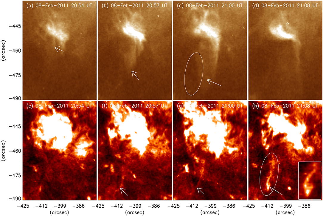
Figure 4. AIA 193 top (a–d) and 304 Å bottom (e–h) images showing the evolution of the jet observed on 2011 February 8 marked by white arrows could be produced by KHI. For the better visibility of the jet, we have saturated the image at the foot-point. The ellipse in the (c,h) represents the east edge of the jets. In 304 Å at ~21:08 UT we have observed the blob structures at the eastern boundary. The enlarged view of the blobs is shown in the inset in (h).

According to Young and Muglach (2014a) estimations, the jet is extended for H = 30 Mm with a width of Δℓ = 15 Mm. The jet duration is 25 min and the bright point is not significantly disrupted by the jet occurrence. The jet n is $n_{\text{i}}=1.7\times 10^8$ cm⁻³, while that of the surrounding coronal plasma we assume to be $n_{\text{e}}=1.5\times 10^8$ cm⁻³. The jet temperature is T_i = 1.7 MK and the environment one is T_e = 2.0 MK. The jet axial velocity is U_z = 250 km s⁻¹ and the rotational one is U_ϕ = 90 km s⁻¹. Assuming a magnetic field twist ε₁ = 0.025 and B_e = 3 G, from Equation (3), we obtain η = 0.882, v_Ai = 494.7 km s⁻¹ (Alfvén speed in the environment is v_Ae = 534.0 km s⁻¹), and b = 1.014. We note, that while in the derivation of Equation (11) we have neglected the thermal pressures, here, in using Equation (3), we kept them. If we anticipate that the shortest unstable wavelength is equal to 7.5 Mm (with k_za = 2π), the mode number m whose instability range would accommodate the aforementioned wavelength, according to inequality (15) must be at least |m| = 71. The numerics show that the suitable m is |m| = 65. Thus, the input parameters for obtaining the numerical solutions to Equation (11) are: m = 65, η = 0.882, ε₁ = 0.025, ε₂ = 0.36 (= 90/250), b = 1.014, and M_A = 0.505 (≅250.0/494.7). The results are illustrated in Figure 5. Along with λ_KH = 7.5 Mm (purple lines), we have calculated the KHI characteristics also for λ_KH = 15 Mm (at k_za = π) (green lines), and they are

$\begin{array}{l}{\gamma }_{\text{KH}}=72.0\times 10^{-3}{\text{s}}^{-1},{\tau }_{\text{KH}}\cong 1.5\text{ min},v_{\text{ph}}\cong 618\text{ km }{\text{s}}^{-1},\\ \text{for}{\lambda }_{\text{KH}}=7.5\text{ Mm},\end{array}$

and

$\begin{array}{l}{\gamma }_{\text{KH}}\cong 342.75\times 10^{-3}{\text{s}}^{-1},{\tau }_{\text{KH}}\cong 0.3\text{ min},v_{\text{ph}}\cong 1106\text{ km }{\text{s}}^{-1},\\ \text{ for}{\lambda }_{\text{KH}}=15\text{ Mm}.\end{array}$

It is seen from the left panel that the unstable m = 65 MHD waves are generally super-Alfvénic. Since the instability developing times of the m = 65 mode are relatively short, that is, much less than the jet lifetime of 25 min, we can conclude that the KHI in this jet is relatively fast.

FIGURE 5

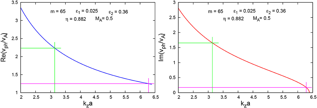
Figure 5. (Left) Dispersion curve of the m = 65 MHD mode propagating along a twisted cool coronal hole jet at η = 0.882, b = 1.014, M_A = 0.5, ε₁ = 0.025, and ε₂ = 0.36. (Right) Normalized growth rate curve of the m = 65 MHD mode computed at the same input parameters as in the left panel. The crosses of purple and green lines yield the normalized values of the wave phase velocity and the wave growth rate at the two unstable wavelengths of 7.5 and 15 Mm, respectively.

With the increase in the parameter ε₁, the instability region, as seen from the right panel of Figure 6, becomes narrower and at the lower limit (k_za)_lhs = π/2 with ${\epsilon }_1^{\text{cr}}=0.10682$ and M_A = 0.5026 its width is equal to zero. In other words, there is no longer instability. Therefore, the critical azimuthal magnetic field that suppresses the KHI is $B_{\text{i}\varphi }^{\text{cr}}\cong 0.3$ G—obviously a relatively small value.

FIGURE 6

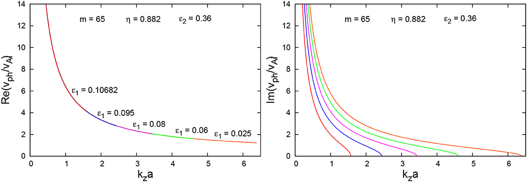
Figure 6. (Left) Dispersion curves of the unstable m = 65 MHD mode propagating along a twisted cool jet in a coronal hole at η = 0.882, ε₂ = 0.36, and the following values of ε₁ (from right to left): 0.025, 0.06, 0.08, 0.095, and 0.10682 (red curve in the right plot). Alfvén Mach numbers for these curves are, respectively 0.505, 0.505, 0.504, 0.503, and 0.5026. (Right) Growth rates of the unstable m = 65 mode for the same input parameters. The azimuthal magnetic field that corresponds to ${\epsilon }_1^{\text{cr}}=0.10682$ (the instability window with zero width) and stops the KHI onset is equal to 0.3 G.

4.3. Kelvin–Helmholtz Instability in a Jet Emerging From a Filament Eruption

Filippov et al. (2015) observationally studied three jets events originated from the active region NOAA 11715 (located on the west limb) on 2013 April 10–11. These authors claim that the jets originated from the emergence of a filament having a null-point (inverted Y) topology. We have considered the second event described in that paper for a detailed study. The jet electron number density, n_i, and electron temperature, T_i, both listed in Table 1, have been calculated by us using the techniques elaborated by Aschwanden et al. (2013). This technique requires the data from the six 94, 131, 171, 193, 211, and 335 Å AIA/SDO EUV channels. In addition to the electron number densities and electron temperatures in the jet and surrounding plasma, we have also estimated the jet width as Δℓ ≈ 30 Mm, its height as H = 180 Mm, and have found the jet lifetime to be 30 min. The two important parameters, axial and azimuthal velocities, according to the observations, are U_z = 100 and U_ϕ = 180 km s⁻¹, respectively. The time evolution of the jet in AIA 304 Å is shown in Figure 7 and we have observed vortex type structures in the eastern side of the jet, which are indicated by arrows. These structures implicitly indicate for occurrence of KHI.

FIGURE 7

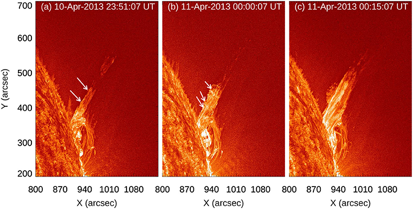
Figure 7. Evolution of the jet associated with a filament eruption observed on 2013 April 10–11 in AIA 304 Å. The structure shown by arrows can be due to the KHI.

With the typical n and T_e (see Table 1), rotating velocity U_ϕ = 180 km s⁻¹, assumed B_e = 6 G, and ε₁ = 0.1, Equation (3) yields η = 0.864, b = 4.36, and v_Ai = 44.00 km s⁻¹ (for comparison, the Alfvén speed in the environment is v_Ae = 206.3 km s⁻¹). We note that the choice of ε₁ was made taking into account the fact that the inclination of the treads of the jet in the event on 2013 April 10, detected by SDO/AIA, yields a relationship between B_iϕ and B_iz, which was evaluated as ε₁ ≈ 0.1. If we assume that the shortest unstable wavelength is λ_KH = 12 Mm, which is located at k_za = 2.5π on the k_za-axis, from inequality (15) we find that a MHD wave with |m| = 12 would provide an instability region, accommodating the non-dimensional k_za = 2.5π. It turns out that a suitable mode number is m = 10. The wave dispersion and growth rate diagrams are shown in Figure 8. In that instability range one can also find the instability characteristics at k_za = 2π, which corresponds to λ_KH = 15 Mm. The input parameters for finding the solutions to Equation (10) are: m = 10, η = 0.864, ε₁ = 0.1, ε₂ = 1.8, b = 4.36, and M_A = 2.27 (= 100/44) The KHI parameters at the aforementioned wavelengths are as follows:

$\begin{array}{l}{\gamma }_{\text{KH}}\cong 33.51\times 10^{-3}{\text{s}}^{-1},{\tau }_{\text{KH}}\cong 3.1\text{ min},v_{\text{ph}}\cong 170\text{ km }{\text{s}}^{-1},\\ \text{ for}{\lambda }_{\text{KH}}=12\text{ Mm},\end{array}$

and

$\begin{array}{l}{\gamma }_{\text{KH}}\cong 46.06\times 10^{-3}{\text{s}}^{-1},{\tau }_{\text{KH}}\cong 2.3\text{ min},v_{\text{ph}}\cong 198\text{ km }{\text{s}}^{-1},\\ \text{ for}{\lambda }_{\text{KH}}=15\text{ Mm}.\end{array}$

The KHI developing or growth times seem reasonable and the wave phase velocities are super-Alfvénic ones.

FIGURE 8

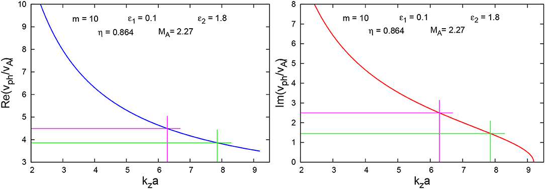
Figure 8. (Left) Dispersion curve of the m = 10 MHD mode propagating along a twisted incompressible emerging from a filament eruption jet at η = 0.864, b = 4.36, M_A = 2.27, ε₁ = 0.1, and ε₂ = 1.8. (Right) Normalized growth rate curve of the m = 10 MHD mode computed at the same input parameters as in the left panel. The crosses of green and purple lines yield the normalized values of the wave phase velocity and the wave growth rate at the two unstable wavelengths of 12 and 15 Mm, respectively.

It is intriguing to see how the width of the instability range will shorten as the magnetic field twist ε₁ is increased. Our numerical computations indicate that for a noticeable contraction of the instability window one should change the magnitude of ε₁ with relatively large steps. The results of such computations are illustrated in Figure 9. It is necessary to underline that at values of ε₁ close to 1, (i) β_i becomes <1 and the jet has to be treated as a cool medium, which implies a new wave dispersion relation and probably a higher wave mode number, m; (ii) one cannot use ε₁ > 1, because in that case the instability is of another kind, namely kink instability (Lundquist, 1951; Hood and Priest, 1979; Zaqarashvili et al., 2014). At this “pathological” case, one cannot reach the lower limit of the instability range, (k_za)_lhs = 0.524, and consequently we are unable to evaluate that azimuthal magnetic field, $B_{\varphi }^{\text{cr}}$, which will stop the KHI onset!

FIGURE 9

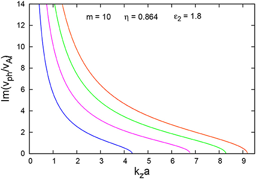
Figure 9. Growth rate curves of the unstable m = 10 MHD mode propagating along a twisted incompressible emerging from a filament eruption jet at η = 0.864, ε₂ = 1.8, and the following values of ε₁ (from right to left): 0.1 (orange), 0.6 (green), 0.8 (purple), and 0.9 (blue).

4.4. Kelvin–Helmholtz Instability in a Spinning Macrospicule

As we have mentioned in section 1, Pike and Mason (1998) did a statistical study of the dynamics of solar transition region features, like macrospicules. These features were observed on the solar disk and also on the solar limb by using data from the Coronal Diagnostic Spectrometer (CDS) onboard SOHO. In addition, in their article, Pike and Mason (1998) discussed the unique CDS observations of a macrospicule first reported by Pike and Harrison (1997) along with their own (Pike and Mason) observations from the Normal Incidence Spectrometer (NIS). This spectrometer covers the wavelength range from 307 to 379 Å and that from 513 to 633 Å using a microchannel plate and CCD combination detector. The details of macrospicule events observed near the limb are given in Table 1 in Pike and Mason, 1998, while those of macrospicule events observed on the disk are presented in Table 2. The main finding in the study of Pike and Mason (1998) was the rotation in these features based on the red and blue shifted emission on either side of the macrospicule axes. According to the authors, the detected rotation assuredly plays an important role in the dynamics of the transition region. Using the basic observational parameters obtained by Pike and Mason (1998), Zhelyazkov and Chandra (2019) examined the conditions for KHI rising in the macrospicule. Let us discuss that study as follows.

Our (Zhelyazkov and Chandra, 2019) choice for modeling namely the macrospicule observed on 1997 March 8 at 00:02 UT (see Table 2 in Pike and Mason, 1998) was made taking into account the fact that this macrospicule possesses the basic characteristics of the observed over the years tornado-like jets—the axial velocity of the jet was U_z = 75 km s⁻¹, while its rotating speed, we evaluate to be U_ϕ = 40 km s⁻¹. For the other characteristics of the macrospicule such as lifetime, maximum width, average flow velocity, and maximum length or height, we used some average values obtained from a huge number of observations and specified in Kiss et al. (2017) as 16.75 ± 4.5 min, 6.1 ± 4 Mm, 73.14 ± 25.92 km s⁻¹, and 28.05 ± 7.67 Mm, respectively. For our study here, we take the macrospicule width to be Δℓ = 6 Mm, its height H = 28 Mm, and lifetime of the order on 15 min. The basic macrospicule physical parameters (see Table 1) with U_ϕ = 40 km s⁻¹, ε₁ = 0.005, and B_e = 5 G yield (using Equation 3) η = 0.1, Alfvén speed v_Ai = 60.6 km s⁻¹ (while in the surrounding plasma we have v_Ae ≅ 345 km s⁻¹), and b = 1.798. The excited MHD mode, whose instability window would contain a λ_KH = 3 Mm, is |m| = 52. Performing the numerical computations with the input parameters: m = 52, η = 0.1, ε₁ = 0.005, ε₂ = 0.53 (= 40/75), b = 1.798, and M_A = 1.24 (= 75/60.6), we get plots very similar to those pictured in Figure 2, which (the plots) allow us to find the KHI characteristics for the two wavelengths of 3 and 5 Mm, exactly

$\begin{array}{l}{\gamma }_{\text{KH}}\cong 48.38\times 10^{-3}{\text{s}}^{-1},{\tau }_{\text{KH}}\cong 2.2\text{ min},v_{\text{ph}}\cong 361\text{ km }{\text{s}}^{-1},\\ \text{ for}{\lambda }_{\text{KH}}=3\text{ Mm},\end{array}$

and

$\begin{array}{l}{\gamma }_{\text{KH}}\cong 184.8\times 10^{-3}{\text{s}}^{-1},{\tau }_{\text{KH}}\cong 0.57\text{ min},v_{\text{ph}}\cong 556\text{ km }{\text{s}}^{-1},\\ \text{ for}{\lambda }_{\text{KH}}=5\text{ Mm}.\end{array}$

One observes that at both unstable wavelengths the corresponding phase velocities are supper-Alfvénic. Moreover, the two growth times of 2.2 and ~0.6 min seem reasonable bearing in mind the fact that the macrospicule lifetime is about 15 min, which implies that the KHI at the selected wavelengths is rather fast. The $B_{\text{i}\varphi }^{\text{cr}}$ that suppresses the KHI onset, equals 0.57 G and was calculated with ${\epsilon }_1^{\text{cr}}=0.202085$ and M_A = 1.2119. Our study (Zhelyazkov and Chandra, 2019) shows that a decrease in the background magnetic field to B_e = 4.8 G would require the excitation of MHD wave with mode number m = 48, at which the KHI characteristics at the wavelengths of 3 and 5 Mm are very close to those obtained with m = 52.

5. Summary and Outlook

In this article, we have studied the emerging of KHI in four different spinning solar jets (standard and blowout coronal hole jets, jet emerging from a filament eruption, and rotating macrospicule) due to the excitation of high-mode (m ⩾ 2) MHD waves traveling along the jets. First and foremost, we model each jet as a vertically moving with velocity U cylindrical twisted magnetic flux tube with radius a. There are four basic steps in the modeling as follows:

• Topology of jet–environment magnetic and velocity fields For simplicity, we assume that the plasma densities of the jet and its environment, ρ_i and ρ_e, respectively, are homogeneous. Generally they are different and the density contrast is characterized by the ratio ρ_e/ρ_i = η. The twisted internal magnetic and velocity fields are supposed to be uniform, that is, represented in cylindrical coordinates, (r, ϕ, z), by the vectors B_i = (0, B_iϕ(r), B_iz) and U = (0, U_ϕ(r), U_z), where their azimuthal components are considered to be linear functions of the radial position r, viz. B_iϕ(r) = Ar and U_ϕ(r) = Ωr, where A and Ω (the azimuthal jet velocity) are constants. We note that B_iz and U_z are also constants. It is convenient the twists of the magnetic field and the flow velocity of the jet to be characterized by the two numbers ε₁ = B_iϕ(a)/B_iz ≡ Aa/B_iz and ε₂ = U_ϕ(a)/U_z ≡ Ωa/U_z, respectively. Note that Ωa is the jet rotational speed U_z. The surrounding coronal or chromospheric plasma is assumed to be immobile and embedded in a constant magnetic field B_e = (0, 0, B_e). In our study, the density contrast, η, varies from 0.1 to 0.9, the magnetic field twist, ε₁, can have a wide range of magnitudes from 0.005 to 0.95 (it has to be less than 1 in order to avoid the rising of the kink instability), while the velocity twist parameter, ε₂, is fixed by the observationally measured rotational and axial speeds.

• Listing of the basic physical parameters and determination of plasmas betas In general, at a fixed density contrast, the plasma beta is controlled by the magnetic field (inside or outside the magnetic flux tube) and the electron temperatures of the jet and surrounding plasma. The values of these physical parameters should satisfy the total pressure balance Equation (3) at all levels (equilibrium and perturbational). Our practice is to fix B_e, and using Equation (3) to determine the internal Alfvén speed defined as $v_{\text{Ai}}=B_{\text{i}z}/\sqrt{\mu {\rho }_{\text{i}}}$. It is worth underlying that the usage of Equation (3) requires the specification of ε₁. In our four cases, for finding the KHI characteristics, we took ε₁ to be equal to 0.005, 0.025, or 0.1. The electron temperatures in the jets are from 500,000 K for the macrospicule to 2.0 MK in the jet emerging from a filament eruption. The electron temperatures of surrounding plasmas are 2.14 MK in the active solar region (Filippov et al., 2015), 2.0 MK in the blowout coronal hole jet (Young and Muglach, 2014a), and 1.0 MK in the environments of the standard coronal hole jet (Chen et al., 2012) and the macrospicule. With background magnetic fields of 3–6 G, rotating velocities of 40–180 km s⁻¹, and ε₁ = 0.005, the total pressure balance Equation (3) yields plasma betas of the first, third, and fourth jets greater than 1 and those of the environments and the internal medium of the second jet much <1 (see Table 1). With these plasma beta values one can consider the media of the standard coronal hole jet, the rotating jet emerging from a filament eruption, and microspicule as nearly incompressible plasmas, while the internal medium of the blowout coronal hole jet and the surrounding magnetized plasma in the four cases can be treated as a cool medium (Zank and Matthaeus, 1993).

• Solving of the wave dispersion relation and finding the KHI characteristics For finding the solutions to the MHD wave dispersion Equations (10) or (11), which are a slight modification of the ‘basic’ dispersion relation derived in Zaqarashvili et al., 2015, it is necessary to specify the following input data: the wave mode number, m, the density contrast, η, the two twist parameters ε₁ and ε₂, the magnetic fields ratio, b [obtainable from Equation (3)], and the Alfvén Mach number M_A = U_z/v_Ai. The roots of the dispersion Equations (10) or (11) are the normalized wave phase velocity and instability growth rate as functions of the non-dimensional wavenumber k_za. From plots which graphically represent the found solutions, one obtains at the anticipated wavelengths (given by their k_za-values on the horizontal k_za-axes) the corresponding Re(v_ph/v_Ai) and Im(v_ph/v_Ai) values. From them, one can find in absolute units the KHI growth rate, γ_KH, the instability developing or growth time, τ_KH = 2π/γ_KH, and the corresponding wave phase velocity, v_ph. The MHD wave mode numbers at which we were able to calculate the instability characteristics at wavelengths comparable to the radius or width of the jet are between 10 and 65 and the KHI growth times at those wavelengths are of the order on a few minutes, generally in good agreement with the observations. It is curious to note that in searching KHI growth times of the order on few seconds, when studying the dynamics and stability of small-scale rapid redshifted and blueshifted excursions, appearing as high-speed jets in the wings of the Hα line, Kuridze et al. (2016) had to assume the excitation of MHD waves with mode numbers up to 100. A typical property of the instability developing times, owing to the shape of the plotted dispersion curves, is that with increasing the examined wavelength the growth times become shorter—for instance, at λ_KH = 10 Mm the KHI developing time in the coronal hole jet (Chen et al., 2012) is around 4.5 min, while at λ_KH = 12 Mm it is equal to ≅2.1 min. A change in B_e can influence the MHD mode number m, which would yield an instability region similar or identical to that seen in Figure 2. It is necessary to mention that the width of the instability range except by changing the MHD wave mode number, m, can be regulated by increasing or diminishing the parameter ε₁.

• Finding the critical azimuthal magnetic field which suppresses the emergence of KHI It was numerically established, that any increase in ε₁ yields to the shortening of the instability range. This observation implies that there should exist some critical ε₁, at which the upper limit of the instability range coincides with the lower one—in that case the width of the instability window is zero, which means that there is no longer any instability. With such an ${\epsilon }_1^{\text{cr}}$, one can calculate the $B_{\text{i}\varphi }^{\text{cr}}$, which stops the KHI appearance. For the rotating blowout coronal hole jet this $B_{\text{i}\varphi }^{\text{cr}}$ is relatively small—it is equal to ≈0.3 G, while for the standard coronal hole jet it is 1.4 G. It is worth noticing that due to the specific parameters of the jet emerging from a filament eruption, we were unable to find a $B_{\text{i}\varphi }^{\text{cr}}$, which would stop the KHI onset because with values of ε₁ close to 1 our dispersion relation becomes inappropriate (the internal medium being nearly incompressible becomes a cool one) and we cannot calculate that ε₁ at which the lower limit, (k_za)_lhs = 0.524, can be reached (see Figure 9).

In this article, we also corrected the total pressure balance equation used in Zhelyazkov et al. (2018) and Zhelyazkov and Chandra (2018), which turns out to be erroneous. The true total balance equation is given by Equation (3). In fact, the corrected pressure balance equation, used here, changes the mode numbers at which the KHI occurs, namely from m = 12 to m = 11 for the coronal hole jet and from m = 18 to m = 10 for the rotating jet emerging from a filament eruption. The computed KHI developing or growth times in the aforementioned articles, nonetheless, are not changed noticeably—they are of the same order with these computed in this paper. In addition, there is another improvement issue, scilicet when studying how the increasing ε₁ shortens the instability region, one has to apply Equation (3) for obtaining the appropriate values of b = B_e/B_iz and $v_{\text{Ai}}=B_{\text{i}z}/\sqrt{\mu {\rho }_{\text{i}}}$, and subsequently M_A = U_z/v_Ai. Thus, one can claim that Equation (3) plays an important role in the numerical studies of the KHI in various solar jets.

Our approach in investigating the KHI in rotating twisted solar jets can be improved in the following directions: (i) to assume some radial profile of the plasma density of the jet, which immediately will require additional study on the occurrence of continuous spectra and resonant wave absorption (Goedbloed and Poedts, 2004), alongside to see to what extent these phenomena will influence the instability growth times; (ii) to investigate the impact of the non-linear azimuthal magnetic and velocity fields radial profiles on the emergence of KHI; and (iii) to derive a MHD wave dispersion relation without any simplifications like considering the jet and its environment as incompressible or cool plasmas—this will show how the compressibility will change the picture. We should also not forget that the non-linearity, as Miura and Pritchett (1982) and Miura (1984) claim, can lead to the saturation of the KHI growth, and to formation of non-linear waves. Nevertheless, even in its relatively simple form, our way of investigating the conditions under which the KHI develops is flexible enough to explore that event in any rotating solar jet in case that the basic physical and geometry parameters of the jet are provided by observations.

Author Contributions

IZh wrote the substantial parts of the manuscript. RJ wrote the Introduction section and prepared three figures associated with the observations. RC contributed by writing the parts devoted to observations, as well as in the careful proofreading of the text.

Funding

The work of IZh and RC was supported by the Bulgarian Science Fund contract DNTS/INDIA 01/7. RJ was funded by the Department of Science and Technology, New Delhi, India as an INSPIRE fellow. RC was also supported from the SERB-DST project no. SERB/F/7455/2017-17.

Conflict of Interest Statement

The authors declare that the research was conducted in the absence of any commercial or financial relationships that could be construed as a potential conflict of interest.

Acknowledgments

We thank Professor Teimuraz V. Zaqarashvili for useful discussions and are deeply grateful to the reviewers for their constructive comments.

References

Ajabshirizadeh, A., Ebadi, H., Vekalati, R. E., and Molaverdikhani, K. (2015). The possibility of Kelvin-Helmholtz instability in solar spicules. Astrophys. Space Sci. 357:33. doi: 10.1007/s10509-015-2277-8

CrossRef Full Text | Google Scholar

Aschwanden, M. J., Boerner, P., Schrijver, C. J., and Malanushenko, A. (2013). Automated temperature and emission measure analysis of coronal loops and active regions observed with the atmospheric imaging assembly on the solar dynamics observatory (SDO/AIA). Sol. Phys. 283, 5–30. doi: 10.1007/s11207-011-9876-5

CrossRef Full Text | Google Scholar

Barbulescu, M., and Erdélyi, R. (2018). Magnetoacoustic waves and the Kelvin–Helmholtz instability in a steady asymmetric slab. I: the effects of varying density ratios. Solar Phys. 293:86. doi: 10.1007/s11207-018-1305-6

PubMed Abstract | CrossRef Full Text | Google Scholar

Bennett, S. M., and Erdélyi, R. (2015). On the statistics of macrospicules. Astrophys. J. 808:135. doi: 10.1088/0004-637X/808/2/135

CrossRef Full Text | Google Scholar

Bodo, G., Mamatsashvili, G., Rossi, P., and Mignone, A. (2016). Linear stability analysis of magnetized jets: the rotating case. Mon. Not. R. Astron. Soc. 462, 3031–3052. doi: 10.1093/mnras/stw1650

CrossRef Full Text | Google Scholar

Bodo, G., Rosner, R., Ferrari, A., and Knobloch, E. (1989). On the stability of magnetized rotating jets: the axisymmetric case. Astrophys. J. 341, 631–649. doi: 10.1086/167522

CrossRef Full Text | Google Scholar

Bodo, G., Rosner, R., Ferrari, A., and Knobloch, E. (1996). On the stability of magnetized rotating jets: the nonaxisymmetric modes. Astrophys. J. 470, 797–805. doi: 10.1086/177910

CrossRef Full Text | Google Scholar

Bogdanova, M., Zhelyazkov, I., Joshi, R., and Chandra, R. (2018). Solar jet on 2014 April 16 modeled by Kelvin–Helmholtz instability. New Astron. 63, 75–87. doi: 10.1016/j.newast.2018.03.001

CrossRef Full Text | Google Scholar

Bondenson, A., Iacono, R., and Bhattacharjee, A. (1987). Local magnetohydrodynamic instabilities of cylindrical plasma with sheared equilibrium flows. Phys. Fluids 30, 2167–2180. doi: 10.1063/1.866151

CrossRef Full Text | Google Scholar

Chandra, R., Mandrini, C. H., Schmieder, B., Joshi, B., Cristiani, G. D., and Cremades, H., et al. (2017). Blowout jets and impulsive eruptive flares in a bald-patch topology. Astron. Astrophys. 598:A41. doi: 10.1051/0004-6361/201628984

CrossRef Full Text | Google Scholar

Chandrasekhar, S. (1961). Hydrodynamic and Hydromagnetic Stability. Oxford: Clarendon Press.

Google Scholar

Chen, H.-D., Zhang, J., and Ma, S.-L. (2012). The kinematics of an untwisting solar jet in a polar coronal hole observed by SDO/AIA. Res. Astron. Astrophys. 12, 573–583. doi: 10.1088/1674-4527/12/5/009

CrossRef Full Text | Google Scholar

Cheremnykh, O., Cheremnykh, S., Kozak, L., and Kronberg, E. (2018a). Magnetohydrodynamic waves and the Kelvin-Helmholtz instability at the boundary of plasma mediums. Phys. Plasmas 25:102119. doi: 10.1063/1.5048913

CrossRef Full Text | Google Scholar

Cheremnykh, O., Fedun, V., Ladikov-Roev, Y., and Verth, G. (2018b). On the stability of incompressible MHD modes in magnetic cylinder with twisted magnetic field and flow. Astrophys. J. 866:86. doi: 10.3847/1538-4357/aadb9f

CrossRef Full Text | Google Scholar

Cranmer, S. R., Asgari-Targhi, M., Miralles, M. P., Raymond, J. C., Strachan, L., and Tian, H., et al. (2015). The role of turbulence in coronal heating and solar wind expansion. Philos. Trans. R. Soc. A 373:20140148. doi: 10.1098/rsta.2014.0148

PubMed Abstract | CrossRef Full Text | Google Scholar

Culhane, J. L., Harra, L. K., James, A. M., Al-Janabi, K., Bradley, L. J., and Chaudry, R. A., et al. (2007). The EUV imaging spectrometer for Hinode. Sol. Phys. 243, 19–61. doi: 10.1007/s01007-007-0293-1

CrossRef Full Text | Google Scholar

Curdt, W., and Tian, H. (2011). Spectroscopic evidence for helicity in explosive events. Astron. Astrophys. 532:L9. doi: 10.1051/0004-6361/201117116

CrossRef Full Text | Google Scholar

De Pontieu, B., Carlsson, M., Rouppe van der Voort, L. H. M., Rutten, R. J., Hansteen, V. H., and Watanabe, H. (2012). Ubiquitous torsional motions in Type II spicules. Astrophys. J. 752:L12. doi: 10.1088/2041-8205/752/1/L12

CrossRef Full Text | Google Scholar

De Pontieu, B., Title, A. M., Lemen, J. R., Kushner, G. D., Akin, D. J., and Allard, B., et al. (2014). The interface region imaging spectrograph (IRIS). Solar Phys. 289, 2733–2779. doi: 10.1007/s11207-014-0485-y

CrossRef Full Text | Google Scholar

Domingo, V., Fleck, B., and Poland, A. I. (1995). SOHO: the solar and heliospheric observatory. Space Sci. Rev. 72, 81–84. doi: 10.1007/BF00768758

CrossRef Full Text | Google Scholar

Ebadi, H. (2016). Kelvin-Helmholtz instability in solar spicules. Indian J. Phys. Res. 16, 41–45. doi: 10.18869/acadpub.ijpr.16.3.41

CrossRef Full Text | Google Scholar

Fang, F., Fan, Y., and McIntosh, S. W. (2014). Rotating solar jets in simulations of flux emergence with thermal conduction. Astrophys. J. 789:L19. doi: 10.1088/2041-8205/789/1/L19

CrossRef Full Text | Google Scholar

Filippov, B., Srivastava, A. K., Dwivedi, B. N., Masson, S., Aulanier, G., and Joshi, N. C., et al. (2015). Formation of a rotating jet during the filament eruption on 2013 April 10–11. Mon. Not. R. Astron. Soc. 451, 1117–1129. doi: 10.1093/mnras/stv1039

CrossRef Full Text | Google Scholar

Goedbloed, J. P., and Poedts, S. (2004). Principles of Magnetohydrodynamics: With Applications to Laboratory and Astrophysical Plasmas. Cambridge: Cambridge University Press.

Google Scholar

Goossens, M., Hollweg, J. V., and Sakurai, T. (1992). Resonant behaviour of MHD waves on magnetic flux tubes tiny III. Effect of equilibrium flow. Solar Phys. 138, 233–255. doi: 10.1007/BF00151914

CrossRef Full Text | Google Scholar

Heyvaerts, J., Priest, E. R., and Rust, D. M. (1997). An emerging flux model for the solar flare phenomenon. Astrophys. J. 216, 123–137. doi: 10.1086/155453

CrossRef Full Text | Google Scholar

Hong, J.-C., Jiang, Y.-C., Yang, J.-Y., Zheng, R.-S., Bi, Y., and Li, H.-D., et al. (2013). Twist in a polar blowout jet. Res. Astron. Astrophys. 13, 253–258. doi: 10.1088/1674-4527/13/3/001

CrossRef Full Text | Google Scholar

Hood, A. W., and Priest, E. R. (1979). Kink instability of solar coronal loops as the cause of solar flares. Solar Phys. 64, 303–321. doi: 10.1007/BF00151441

CrossRef Full Text | Google Scholar

Ismayilli, R. F., Dzhalilov, N. S., Shergelashvili, B. M., Poedts, S., and Pirguliyev, M. Sh. (2018). MHD Kelvin-Helmholtz instability in the anisotropic solar wind plasma. Phys. Plasmas 25:062903. doi: 10.1063/1.5032161

CrossRef Full Text | Google Scholar

Joshi, R., Schmieder, B., Chandra, R., Aulanier, G., Zuccarello, F. P., and Uddin, W. (2017). Slippage of jets explained by the magnetic topology of NOAA active region 12035. Solar Phys. 292:152. doi: 10.1007/s11207-017-1176-2

CrossRef Full Text | Google Scholar

Kamio, S., Curdt, W., Teriaca, L., Inhester, B., and Solanki, S. K. (2010). Observations of a rotating macrospicule associated with an X-ray jet. Astron. Astrophys. 510: L1. doi: 10.1051/0004-6361/200913269

CrossRef Full Text | Google Scholar

Kayshap, P., Srivastava, A. K., Murawski, K., and Tripathi, D. (2013). Origin of macrospicule and jet in polar corona by a small-scale kinked flux tube. Astrophys. J. 770:L3. doi: 10.1088/2041-8205/770/1/L3

CrossRef Full Text | Google Scholar

Kiss, T. S., Gyenge, N., and Erdélyi, R. (2017). Systematic variations of macrospicule properties observed by SDO/AIA over half a decade. Astrophys. J. 835:47. doi: 10.3847/1538-4357/aa5272

CrossRef Full Text | Google Scholar

Kiss, T. S., Gyenge, N., and Erdélyi, R. (2018). Quasi-biennial oscillations in the cross-correlation of properties of macrospicules. Adv. Space Res. 61, 611–616. doi: 10.1016/j.asr.2017.05.027

CrossRef Full Text | Google Scholar

Kosugi, T., Matsuzaki, K., Sakao, T., Shimizu, T., Sone, Y., and Tachikawa, S., et al. (2007). The Hinode (Solar-B) Mission: An Overview. Solar Phys. 243, 3–17. doi: 10.1007/s11207-007-9014-6

CrossRef Full Text | Google Scholar

Kuridze, D., Zaqarashvili, T. V., Henriques, V., Mathioudakis, M., Keenan, F. P., and Hanslmeier, A. (2016). Kelvin–Helmholtz instability in solar chromospheric jets: theory and observation. Astrophys. J. 830:133. doi: 10.3847/0004-637X/830/2/133

CrossRef Full Text | Google Scholar

Lemen, J. R., Title, A. M., Akin, D. J., Boerner, P. F., Chou, C., and Drake, J. F., et al. (2012). The Atmospheric Imaging Assembly (AIA) on the Solar Dynamics Observatory (SDO). Solar Phys. 275, 17–40. doi: 10.1007/s11207-011-9776-8

CrossRef Full Text | Google Scholar

Liu, W., Berger, T. E., Title, A. M., and Tarbell, T. D. (2009). An intriguing chromospheric jet observed by Hinode: fine structure kinematics and evidence of unwinding twists. Astrophys. J. 707, L37–L41. doi: 10.1088/0004-637X/707/1/L37

CrossRef Full Text | Google Scholar

Lundquist, S. (1951). On the stability of magneto-hydrostatic fields. Phys. Rev. 83, 307–311. doi: 10.1103/PhysRev.83.307

CrossRef Full Text | Google Scholar

Madjarska, M. S. (2019). Coronal bright points. Living. Rev. Solar Phys. 16:2. doi: 10.1007/s41116-019-0018-8

CrossRef Full Text | Google Scholar

Martínez-Sykora, J., De Pontieu, B., Leenaarts, J., Pereira, T. M. D., Carlsson, M., and Hansteen, V., et al. (2013). A detailed comparison between the observed and synthesized properties of a simulated type II spicule. Astrophys. J. 771:66. doi: 10.1088/0004-637X/771/1/66

CrossRef Full Text | Google Scholar

Mishin, V. V., and Tomozov, V. M. (2016). Kelvin-Helmholtz instability in the solar atmosphere, solar wind and geomagnetosphere. Solar Phys. 291, 3165–3184. doi: 10.1007/s11207-016-0891-4

CrossRef Full Text | Google Scholar

Miura, A., and Pritchett, P. L. (1982). Nonlocal stability analysis of the MHD Kelvin-Helmholtz instability in a compressible plasma. J. Geophys. Res. 87, 7431–7444. doi: 10.1029/JA087iA09p07431

CrossRef Full Text | Google Scholar

Miura, A. (1984). Anomalous transport by magnetohydrodynamic Kelvin-Helmholtz instabilities in the solar wind-magnetosphere interaction. J. Geophys. Res. 89, 801–818. doi: 10.1029/JA089iA02p00801

CrossRef Full Text | Google Scholar

Moore, R. L., Cirtain, J. W., Sterling, A. C., and Falconer, D. A. (2010). Dichtonomy of solar coronal jets: standard jets and blowout jets. Astrophys. J. 720, 757–770. doi: 10.1088/0004-637X/720/1/757

CrossRef Full Text | Google Scholar

Moore, R. L., Sterling, A. C., Falconer, D. A., and Robe, D. (2013). The cool component and the dichotomy, lateral expansion, and axial rotation of solar X-ray jets. Astrophys. J. 769:134. doi: 10.1088/0004-637X/769/2/134

CrossRef Full Text | Google Scholar

Moore, R. L., Sterling, A. C., and Falconer, D. A. (2015). Magnetic untwisting in solar jets that go into the outer corona in polar coronal holes. Astrophys. J. 806:11. doi: 10.1088/0004-637X/806/1/11

CrossRef Full Text | Google Scholar

Murawski, K., Srivastava, A. K., and Zaqarashvili, T. V. (2011). Numerical simulations of solar macrospicules. Astron. Astrophys. 355:A58. doi: 10.1051/0004-6361/201116735

CrossRef Full Text | Google Scholar

Nisticò, G., Bothmer, V., Patsourakos, S., and Zimbardo, G. (2009). Characteristics of EUV coronal jets observed with STEREO/SECCHI. Sol. Phys. 259:87. doi: 10.1007/s11207-009-9424-8

CrossRef Full Text | Google Scholar

Nisticò, G., Bothmer, V., Patsourakos, S., and Zimbardo, G. (2010). Observational features of equatorial coronal hole jets. Ann. Geophys. 28, 687–696. doi: 10.5194/angeo-28-687-2010

CrossRef Full Text | Google Scholar

Panesar, N. K., Sterling, A. C., Moore, R. L., and Chakrapani, P. (2016b). Magnetic flux cancelation as the trigger of solar quiet-region coronal jets. Astrophys. J. 832:L7. doi: 10.3847/2041-8205/832/1/L7

CrossRef Full Text | Google Scholar

Panesar, N. K., Sterling, A. C., and Moore, R. L. (2016a). Homologous jet-driven coronal mass ejections from solar active region 12192. Astrophys. J. 822:L23. doi: 10.3847/2041-8205/822/2/L23

CrossRef Full Text | Google Scholar

Pariat, E., Antiochos, S. K., and DeVore, C. R. (2009). A model for solar polar jets. Astrophys. J. 691, 61–74. doi: 10.1088/0004-637X/691/1/61

CrossRef Full Text | Google Scholar

Pariat, E., Dalmasse, K., DeVore, C. R., Antiochos, S. K., and Karpen, J. T. (2015). Model for straight and helical solar jets. I. Parametric studies of the magnetic field geometry. Astron. Astrophys. 573:A130. doi: 10.1051/0004-6361/201424209

CrossRef Full Text | Google Scholar

Pariat, E., Dalmasse, K., DeVore, C. R., Antiochos, S. K., and Karpen, J. T. (2016). Model for straight and helical solar jets. II. Parametric study of the plasma beta. Astron. Astrophys. 596:A36. doi: 10.1051/0004-6361/201629109

PubMed Abstract | CrossRef Full Text | Google Scholar

Pesnell, W. D., Thompson, B. J., and Chamberlin, P. C. (2012). The Solar Dynamics Observatory (SDO). Solar Phys. 275, 3–15. doi: 10.1007/s11207-011-9841-3

CrossRef Full Text | Google Scholar

Pike, C. D., and Harrison, R. A. (1997). Euv observations of a macrospicule: evidence for solar wind acceleration? Solar Phys. 175, 457–465. doi: 10.1023/A:1004987505422

CrossRef Full Text | Google Scholar

Pike, C. D., and Mason, H. E. (1998). Rotating transition region features observed with the SOHO coronal diagnostic spectrometer. Solar Phys. 182, 333–348.

Google Scholar

Ryu, D., Jones, T. W., and Frank, A. (2000). The magnetohydrodynamic Kelvin-Helmholtz instability: a three-dimensional study of nonliner evolution. Astrophys. J. 545, 475–493. doi: 10.1086/317789

CrossRef Full Text | Google Scholar

Schmieder, B., Guo, Y., Moreno-Insertis, F., Aulanier, G., Yelles Chaouche, L., and Nishizuka, N., et al. (2013). Twisting solar coronal jet launched at the boundary of an active region. Astron. Astrophys. 559:A1. doi: 10.1051/0004-6361/201322181

CrossRef Full Text | Google Scholar

Shen, Y., Liu, Y., Su, J., and Ibrahim, A. (2011). Kinematics and fine structure of an unwinding polar jet observed by the solar dynamic observatory atmospheric imaging assembly. Astrophys. J. 735:L43. doi: 10.1088/2041-8205/735/2/L43

CrossRef Full Text | Google Scholar

Soler, R., Díaz, A. J., Ballester, J. L., and Goossens, M. (2015). Kelvin-Helmholtz instability in partially ionized compressible plasmas. Astrophys. J. 749:163. doi: 10.1088/0004-637X/749/2/163

CrossRef Full Text | Google Scholar

Sterling, A. C., Moore, R. L., Falconer, D. A., and Adams, M. (2015). Small-scale filament eruptions as the driver of X-ray jets in solar coronal holes. Nature 523, 437–440. doi: 10.1038/nature14556

PubMed Abstract | CrossRef Full Text | Google Scholar

Vasheghani Farahani, S., Van Doorsselaere, T., Verwichte, E., and Nakariakov, V. M. (2009). Propagating transverse waves in soft X-ray coronal jets. Astron. Astrophys. 498, L29–L32. doi: 10.1051/0004-6361/200911840

CrossRef Full Text | Google Scholar

Young, P. R., and Muglach, K. (2014a). A coronal hole jet observed with Hinode and the solar dynamics observatory. Publ. Astron. Soc. Japan 66:S12. doi: 10.1093/pasj/psu088

CrossRef Full Text | Google Scholar

Young, P. R., and Muglach, K. (2014b). Solar dynamics observatory and Hinode observations of a blowout jet in a coronal hole. Sol. Phys. 289, 3313–3329. doi: 10.1007/s11207-014-0484-z

CrossRef Full Text | Google Scholar

Zank, G. P., and Matthaeus, W. H. (1993). Nearly incompressible fluids. II: magnetohydrodynamics, turbulence, and waves. Phys. Fluids 5, 257–273. doi: 10.1063/1.858780

CrossRef Full Text | Google Scholar

Zaqarashvili, T. V., Vörös, Z., and Zhelyazkov, R. (2014). Kelvin-Helmholtz instability of twisted magnetic flux tubes in the solar wind Astron. Astrophys. 561:A62. doi: 10.1051/0004-6361/201322808

CrossRef Full Text | Google Scholar

Zaqarashvili, T. V., Zhelyazkov, I., and Ofman, L. (2015). Stability of rotating magnetized jets in the solar atmosphere. I. Kelvin–Helmholtz instability. Astrophys. J. 813:123. doi: 10.1088/0004-637X/813/2/123

CrossRef Full Text | Google Scholar

Zhang, Q. M., and Ji, H. S. (2014). A swirling flare-related EUV jet. Astron. Astrophys. 561:A134. doi: 10.1051/0004-6361/201322616

CrossRef Full Text | Google Scholar

Zhelyazkov, I., Chandra, R., Srivastava, A. K., and Mishonov, T. (2015a). Kelvin–Helmholtz instability of magnetohydrodynamic waves propagating on solar surges. Astrophys. Space Sci. 356:231. doi: 10.1007/s10509-014-2215-1

CrossRef Full Text | Google Scholar

Zhelyazkov, I., Chandra, R., and Srivastava, A. K. (2016). Kelvin–Helmholtz instability in an active region jet observed with Hinode. Astrophys. Space Sci. 361:51. doi: 10.1007/s10509-015-2639-2

CrossRef Full Text | Google Scholar

Zhelyazkov, I., Chandra, R., and Srivastava, A. K. (2017). Modeling Kelvin–Helmholtz instability in soft X-ray solar jets. Adv. Astron. 2017:2626495. doi: 10.1155/2017/2626495

CrossRef Full Text | Google Scholar

Zhelyazkov, I., and Chandra, R. (2018). High mode magnetohydrodynamic waves propagation in a twisted rotating jet emerging from a filament eruption. Mon. Not. R. Astron. Soc. 478, 5505–5513. doi: 10.1093/mnras/sty1354

CrossRef Full Text | Google Scholar

Zhelyazkov, I., and Chandra, R. (2019). Can High-Mode Magnetohydrodynamic Waves propagating in a spinning macrospicule be unstable due to the Kelvin–Helmholtz Instability? Solar Phys. 294:20. doi: 10.1007/s11207-019-1408-8

CrossRef Full Text | Google Scholar

Zhelyazkov, I., Zaqarashvili, T. V., Chandra, R., Srivastava, A. K., and Mishonov, T. (2015b). Kelvin–Helmholtz instability in solar cool surges. Adv. Space Res. 56, 2727–2737. doi: 10.1016/j.asr.2015.05.003

CrossRef Full Text | Google Scholar

Zhelyazkov, I., Zaqarashvili, T. V., Ofman, L., and Chandra, R. (2018). Kelvin–Helmholtz instability in a twisting solar polar coronal hole jet observed by SDO/AIA. Adv. Space Res. 61, 628–638. doi: 10.1016/j.asr.2017.06.003

CrossRef Full Text | Google Scholar

Zhelyazkov, I., and Zaqarashvili, T. V. (2012). Kelvin-Helmholtz instability of kink waves in photospheric twisted flux tubes. Astron. Astrophys. 547:A14. doi: 10.1051/0004-6361/201219512

CrossRef Full Text | Google Scholar

Zhelyazkov, I. (2012). Magnetohydrodynamic waves and their stability status in solar spicules. Astron. Astrophys. 537:A124. doi: 10.1051/0004-6361/201117780

CrossRef Full Text | Google Scholar

Zhelyazkov, I. (2015). On Modeling the Kelvin–Helmholtz instability in solar atmosphere. J. Astrophys. Astr. 36, 233–254. doi: 10.1007/s12036-015-9332-2

CrossRef Full Text | Google Scholar