 Matthew Allcock
 Daria Shukhobodskaia
 Noémi Kinga Zsámberger
 Robert Erdélyi
- 1Solar Physics and Space Plasma Research Centre, School of Mathematics and Statistics, University of Sheffield, Sheffield, United Kingdom
- 2Institute of Physics, University of Debrecen, Debrecen, Hungary
- 3Doctoral School of Physics, University of Debrecen, Debrecen, Hungary
- 4Department of Astronomy, Eötvös L. University, Budapest, Hungary
Diagnosing the solar atmospheric plasma is one of the major challenges in solar physics. Magnetohydrodynamic (MHD) waves, by means of applying the powerful concept of solar magneto-seismology (SMS), provide a tool to obtain diagnostic insight into the magnetized solar plasma in MHD waveguides. This paper provides a road-map of simple but applicable models of solar atmospheric waveguides in the framework of Cartesian geometry. We focus on exploiting the diagnostic potential of waveguide asymmetry and consider the effects of steady flow. In particular, the dispersion relation describing linear MHD wave propagation along a multi-layered MHD waveguide is derived. Aiming at lower solar atmospheric applications of SMS, the special case of a single magnetic slab embedded in an asymmetric magnetized plasma environment is revisited. As a proof of concept, the Amplitude Ratio Method is used to make a seismological estimate of the local Alfvén speed in several chromospheric fibrils that exhibit asymmetric oscillations. Absolute ratios of boundary oscillations between 1.29 and 3.42 are detected and, despite the significant errors expected, the local Alfvén speed estimates agree with previously derived estimates from magnetic field extrapolations. Finally, the effects of asymmetric shear flows present in these slab MHD waveguides are considered as a suitable model of Kelvin-Helmholtz instability initiation that is applicable, for example, to coronal mass ejection flanks.
1. Introduction
Over the past few decades, vast improvements in solar telescope technology, with the likes of both space-borne instrumentation, e.g., Solar and Heliospheric Observatory (SoHO), Solar Dynamics Observatory (SDO), and Interface Region Imaging Spectograph (IRIS), and ground-based solar observing facilities, e.g., Dunn Solar Telescope (DST) and Swedish Solar Telescope (SST), have enabled us to resolve the fine sub-structure within many of the larger magnetic features that bejewel the solar atmosphere. Considering the development of the next generation of observational mega-projects, such as the rather imminent commencement of the Daniel K. Inouye Solar Telescope (DKIST) and, within a decade, that of European Solar Telescope (EST), this trend looks set to continue, which motivates solar physicists to fill the gaps in theoretical understanding.
Magnetohydrodynamic (MHD) waves are a key in our understanding of the physical processes in the hot solar plasma. MHD waves are not only a mechanism to transfer non-thermal energy between distant locations in the solar plasma, that is then dissipated by physical processes that are yet to be fully understood, like resonant absorption (Goossens et al., 2011), phase mixing (Heyvaerts and Priest, 1983), non-linear shock damping (Ballai and Ruderman, 2011), rather, they are also excellent tools to be exploited for plasma diagnostics by solar magneto-seismology (SMS) (see the reviews by Andries et al., 2009; Ruderman and Erdélyi, 2009; Mathioudakis et al., 2013). SMS employs the measured properties of MHD waves, e.g., amplitude, frequency, and phase speed, and, using a suitable inversion, yields information about the waveguide properties that are often very hard to measure (e.g., magnetic field, gravity, magnetic scale heights, or density).
There are two geometric building-blocks that are popular to model solar atmospheric waveguides: the cylindrical flux tube and the magnetic slab waveguides. The present work focuses on the latter, which can be used in the first approximation to model a wide variety of solar atmospheric structures, including prominences, magnetic bright points, light bridges and their corresponding light walls, coronal hole boundary layers, the flank structure of coronal mass ejections, as well as several magnetospheric regions. First studied as an interface between two semi-infinite plasmas (Roberts, 1981b), the currently frequently used and popular format of the theory of MHD wave propagation in Cartesian geometry has been developed to describe magnetic slabs embedded in symmetric (Roberts, 1981a; Edwin and Roberts, 1982) and asymmetric environments (Allcock and Erdélyi, 2017; Zsámberger et al., 2018), and multi-layered plasmas (Ruderman, 1992; Shukhobodskaia and Erdélyi, 2018). Collective standing modes of a multi-layered Cartesian waveguide modeling multi-fibril prominence oscillations (Díaz et al., 2005; Díaz and Roberts, 2006) and coronal loop oscillations (Luna et al., 2006) have been studied. MHD wave theory in Cartesian waveguides has been explored in terms of SMS by Roberts et al. (1984), and more recently by Allcock and Erdélyi (2018).
Aside from providing a description and nomenclature of solar atmospheric wave physics, the theoretical studies have driven progress in SMS. The asymmetric environment of solar waveguides has been theoretically proposed as a proxy for local inhomogeneity, e.g., in the magnetic field, density, and temperature. This inhomogeneity, through the Amplitude Ratio and the Minimum Perturbation Shift Methods, can be exploited for SMS (Allcock and Erdélyi, 2018). With the sub-structure resolution that these techniques require being reached by some of the currently available instrument suits for solar atmospheric waveguide structures, we are now able to apply these techniques.
The aims of this paper are two-fold. First, we bring together the linear theory of MHD wave propagation in Cartesian waveguides modeled by magnetic steady slab equilibria, focusing on the effects of asymmetry surrounding the slab and steady states representing plasma flows. Secondly, we exploit the SMS diagnostic power of waveguide asymmetry by making the first inversion of the local Alfvén speed in chromospheric fibrils using the Amplitude Ratio Method, an SMS technique that has developed out of asymmetric waveguide theory.
The structure of the paper is as follows. Section 2 introduces a general model of a multi-layered MHD waveguide, for which the dispersion relation for linear magneto-acoustic waves is derived. Special cases of this model are discussed in section 3, including a magnetic slab in an asymmetric non-magnetic environment (section 3.1) and magnetic environment (section 3.2). Section 4 applies these models to the low solar atmosphere, first, to estimate the local Alfvén speed in chromospheric fibrils using solar magneto-seismology (section 4.1), then to present mode identification in high-plasma-beta regions (section 4.2). Section 5 analyses the effects of steady flows on linear MHD perturbations and instabilities of a multi-layered solar plasma.
2. General Multi-layered Waveguide Model
Let us first consider a model of a plasma structured by an arbitrary number of interfaces with different homogeneous magnetic fields, temperatures, and densities, illustrated by Figure 1 in Cartesian geometry. Such a model could be useful for studying linear MHD wave propagation in observed solar atmospheric structures closer to the photosphere, such as magnetic bright points, sunspot light bridges, or light walls.
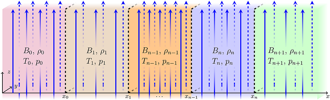
Figure 1. The equilibrium configuration of a layered magnetized plasma. The blue arrows represent the vertical magnetic field, . The kinetic pressure, pj, density, ρj, and temperature, Tj are equilibrium parameters. The subscript j corresponds to the relevant slab and varies from 0 to n + 1.
In what follows, we consider an infinite compressible inviscid structured static plasma with magnetic field , where
We ignore the effects of gravity. We denote the equilibrium kinetic plasma pressure, the density, and temperature by pj, ρj, and Tj, respectively, with subscript j that varies from 0 to n + 1. In total, there are n + 2 regions, all of which, in general, are magnetized.
We assume that the perturbations within the magnetic slab are governed by the ideal MHD equations,
where μ0 is the magnetic permeability of free space, γ is the adiabatic index, variables v = (vx, vy, vz), B, p, and ρ are velocity, magnetic field, kinetic pressure, and density, at time t. The Alfvén and sound speeds in the jth region are vAj = and cj = , respectively. For the system to remain in equilibrium, pressure balance across each interface is required, i.e.,
Equation (2.2) yields the following relation between characteristic speeds and density ratios for any two regions:
We linearize the governing equations by setting, for each variable f, , where fj is the background variable in region j and f′ is the comparatively much smaller perturbation variable, then neglecting terms of quadratic or higher order in perturbation variables. For brevity, we drop the ′ hereafter. We seek plane wave solutions to the linearized governing equations of the form
representing wave propagation in the -direction, where ω is the angular frequency and k is the wavenumber in the -direction. Substituting solutions (2.3) into the system of Equation (2.1), and combining the obtained equations, we derive an ordinary differential equation for representing transverse motions inside the magnetic slab,
where
Note that k = (0, 0, k), the system is homogeneous in the y-direction, and this derivation deals with magnetoacoustic modes and not Alfvén modes, since vy = 0. Now, we assume that the perturbations vanish at infinity, so that as x → ±∞. We note that may take positive or negative values for j from 1 to n. Since the wave amplitudes decay exponentially at infinity, we obtain a general solution of Equation (2.4) given by
where Pi and Qj are constants with i = 0, 1, … n + 1 and j = 1, 2, … n.
The total (kinetic plus magnetic) pressure perturbation, PT(x, t), satisfies the equation
Considering PT(x, t) in a Fourier form, PT(x, t) = , and using Equations (2.1) and (2.7), we obtain
with
Let us now establish appropriate boundary conditions. For physical solutions, the velocity, vx(x, t), and total pressure, PT(x, t), have to be continuous across the boundaries x = xj for j = 0… n. Equations (2.6) and (2.8) give us 2(n + 1) coupled homogeneous algebraic equations:
where Pi and Qj are constant with respect to x. Then, we define Q0 = P0 and Qn+1 = −Pn+1 and rewrite the above boundary conditions into the following compact form
for j = 0, 1, …n. One of the advantages of the above form is its simplistic format which enables it to be used in numerical studies for sufficiently large values of n.
We now rearrange the obtained boundary conditions into the following compact matrix form:
where M is a [2n + 2] × [2n + 2] matrix. The precise form of the matrix is given in Appendix A by Equations (A1)–(A5).
In order to have a non-trivial solution of the system, the determinant of the matrix M must be equal to zero:
Equation (2.13), the general dispersion relation, prescribes the nature of linear MHD waves that can propagate along a static multi-layered waveguide, visualized by Figure 1. The solutions to this equation, given by the angular frequency, ω, as a function of the wavenumber, k, correspond to the eigenfrequencies of the system.
3. Magnetic Slab in an Asymmetric Environment
In order to make analytical progress, we now analyze two special cases of this model in Cartesian geometry, namely, a slab in an asymmetric non-magnetic (section 3.1) and magnetic (section 3.2) homogeneous background plasma. These special cases bring the waveguide model closer to reality as there are several phenomena in the solar atmosphere that can be well modeled by isolated magnetic slabs, including prominences (Arregui et al., 2012), elongated magnetic bright points (Berger and Title, 1996), and light walls (Yang et al., 2015), to name a few.
3.1. Slab in an Asymmetric Non-magnetic Environment
By letting n = 1 and letting the left and right regions be magnetic field free, i.e., B0 = B2 = 0, we reduce the general multi-waveguide structure to a single magnetic slab waveguide in a non-magnetic environment (Figure 2). This waveguide model was studied by Allcock and Erdélyi (2017) and is summarized in this section.
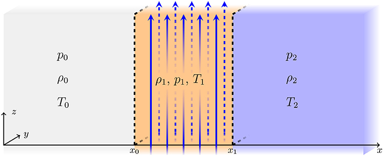
Figure 2. The equilibrium configuration for a magnetic slab in an asymmetric non-magnetic environment.
Under this configuration, the parameters mj and Λj reduce to
and
respectively. By letting x0 = −x1, the matrix form of the dispersion relation, Equation (2.13), reduces to
where Ci = cosh mix1 and Si = sinh mix1, for i = 0, 1, 2. This can be written in non-matrix form as
Using the original notation, the dispersion relation is
This agrees with the dispersion relation derived by Allcock and Erdélyi (2017), with a different subscript labeling.
This has implications for mode identification. Most notably, Table 1 highlights that merely observing cross-sectional oscillation is insufficient for the identification of sausage modes, and merely observing axial oscillation is insufficient for the identification of kink modes. It is a combination of these features and the phase relationship of the boundary oscillations that allows us to accurately identify these modes.
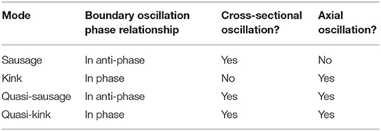
Table 1. The defining characteristics of each category of eigenmode.
The eigenmodes can be further categorized as surface and body modes, depending on whether the solution to the governing equations is evanescent or spatially oscillatory, respectively, within the slab. The main physical implication of this is that the amplitude, or wave power in observations, peaks at the boundaries of the waveguide for surface modes, and at one or more anti-nodes within the waveguide for body modes. Compared to body modes, surface modes are significantly more sensitive to the background plasma and hence the background asymmetry (Allcock and Erdélyi, 2017).
3.2. Slab in an Asymmetric Magnetic Environment
Generalizing the stationary slab embedded in an asymmetric plasma leads us to the model of the magnetic slab embedded in an asymmetric magnetic environment. By letting n = 1, but keeping the magnetic fields in the external regions (unlike in section 3.1), we reduce the general multi-waveguide structure to a single magnetic slab waveguide in an asymmetric homogeneous non-magnetic environment (see Figure 3, and also Zsámberger et al., 2018).
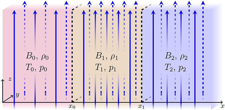
Figure 3. Equilibrium configuration for the magnetic slab in an asymmetric magnetic environment.
In this case, the parameters related to the wavenumbers and the total pressure in all three domains are expressed as
By letting x0 = −x1, we obtain the following dispersion relation
For the full derivation of the dispersion relation using the shifted coordinate system (defined by x0 = −x1, as in section 3.1), see Allcock and Erdélyi (2017) for the externally field-free, and Zsámberger et al. (2018) for the externally magnetic asymmetric slab system. Note also that if we remove the external magnetic fields, Equation (3.7) reduces to the dispersion relation for the externally field-free one-slab system (Equation 3.5).
In general, the solutions of the exact dispersion relation for both the externally field-free and magnetic asymmetric slab systems are the mixed-nature quasi-sausage and quasi-kink modes. Figure 4 shows a few characteristic examples of how the introduction of asymmetry influences the distribution of the transverse velocity perturbation of these eigenmodes under circumstances corresponding to lower solar atmospheric environments.
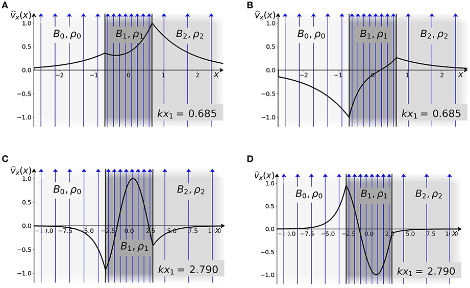
Figure 4. Distribution of the transverse velocity perturbation amplitude () in a strongly magnetized slab and its rarefied asymmetric environment, plotted with solid black curves, as a function of the transverse spatial coordinate, x. Lighter gray shading represents lower background densities, while the blue arrows show the equilibrium magnetic fields, and darker gray shading corresponds to higher background densities. In (A), a slow quasi-kink surface mode, in (B), a slow quasi-sausage surface mode, in (C), a fast quasi-kink body mode of order one, and in (D), a fast quasi-sausage body mode of order one is presented. (A,B) correspond to a thin slab (kx1 = 0.685), while (C,D) represent a wide slab (kx1 = 2.790). These solutions to the dispersion relation (Equation 3.7) were obtained numerically, for a slab system characterized by vA1 = 0.7c1, vA0 = 0.2c1, vA2 = 0.1c1, c0 = 2.23c1, c2 = 1.87c1, ρ0/ρ1 = 0.28, and ρ2/ρ1 = 0.4.
4. Application to the Lower Solar Atmosphere
In this section, we discuss two of the different diagnostic approaches and methods that are possible to pursue with asymmetric slab models. First, we demonstrate the power of the so-called amplitude ratio method with a specific application to surface waves, by briefly outlining the solar magneto-seismology theory of asymmetric MHD waveguides (section 4.1.1), and then applying this theory we estimate the Alfvén speed in several chromospheric fibrils (sections 4.1.2–4.1.7). Then, to illustrate how body waves can be used for diagnostic purposes, we discuss the analytical solutions of the asymmetric slab environment when the kinetic pressure dominates the magnetic pressure, as occurs in the low solar atmosphere (section 4.2).
4.1. Solar Magneto-Seismology With Asymmetric Waveguides
At present, some properties of the solar atmosphere, such as the strength of the magnetic field in the chromosphere and the corona, are very hard to measure directly from emitted or absorbed radiation. To get an estimate of such parameters, we must rely on observables which depend on the unknown parameter by proxy. The asymmetry of solar MHD waveguides is a proxy for the internal magnetic field. In this section, we summarize the Amplitude Ratio Method for solar magneto-seismology of asymmetric waveguides, first derived by Allcock and Erdélyi (2018), and use it to make the first demonstration of an inversion of the local Alfvén speed in the solar atmosphere using asymmetric MHD waves.
4.1.1. Amplitude Ratio Method
MHD waves perturb waveguides in the solar atmosphere in a non-uniform manner. Moreover, the wave power is distributed transversely across the waveguide in a way unique to the mode of oscillation and the background parameters. In particular, asymmetry in the background parameters is mirrored by asymmetry in the transverse distribution of wave power, that is, in the eigenfunction (e.g., Figure 4). One way to quantify this asymmetry is to take the ratio of the signed amplitudes, RA, at each interface of the waveguide, i.e.,
where is the transverse displacement and is evaluated at each boundary, ±x1. Through derivation of the eigenfunctions for each mode (see Allcock and Erdélyi, 2018, for more details), we can express this in terms of the wave parameters and equilibrium parameters,
for quasi-sausage modes, and
for quasi-kink modes. For quasi-sausage modes, the amplitude ratio is negative due to the anti-phase boundary oscillations, and for quasi-kink modes, the amplitude ratio is positive due to the in-phase boundary oscillations. By taking all the other parameters as measured inputs, the internal Alfvén speed, vA1, can be estimated by numerically inverting this equation. In the following application of this SMS technique, we use the Amplitude Ratio Method, as described above, to estimate the Alfvén speed in several chromospheric fibrils.
4.1.2. Alfvén Speed Inversion of Chromospheric Fibrils
The Alfvén speed in the chromospheric quiet Sun is highly inhomogeneous, due to the many magnetic structures that make up the magnetic canopy, and undergoes a steep gradient from 15 km s−1 in photospheric flux tubes to 1, 000 km s−1 in the corona (van Ballegooijen et al., 2011). Techniques including photospheric magnetic field extrapolation and magneto-seismology make up an arsenal of methods for characterizing the chromospheric magnetic field, yet the Alfvén speed in specific chromospheric structures remains hard to determine (Wiegelmann et al., 2014). Here, we apply the Amplitude Ratio Method to diagnose the Alfvén speed in several chromospheric fibrils as a demonstration of a new magneto-seismology technique to add to the picture.
The data were taken from observations close to the disk center with a narrow-band 0.25 ÅHα core (6562.8 Å) filter on the 29th September 2010 using the Rapid Oscillations in the Solar Atmosphere (ROSA) imager on the Dunn Solar Telescope (Jess et al., 2010). The data show a dynamic sea of dark dense fibrils that map, at least partially, the inter-network magnetic field overlying the bright and less dense plasma that permeates the quiet Sun (Leenaarts et al., 2012). The implementation of the Amplitude Ratio Method involves resolving sub-fibril structure, for which the ROSA instrument's high spatial (150 km) and temporal resolution (7.68 s) were necessary and just barely sufficient, with 10-20 pixels across each fibril.
More information about the observations is detailed by Morton et al. (2012), who originally used the same data for the analysis of ubiquitous MHD waves in the chromosphere. They interpreted the observed fibril oscillations as concurrent sausage and kink modes of circular cross-sectional magnetic flux-tubes. In the present analysis, we propose an alternative interpretation that the oscillations are MHD oscillations in asymmetric waveguides. Evidence in favor of the present interpretation comes from the observation that the oscillations in the transverse axial displacement, the cross-sectional width, and the integrated intensity across the fibrils are both in phase and demonstrate a similar phase speed (see Morton et al., 2012). However, we wish to make it clear that this interpretation is taken mainly to demonstrate a new SMS technique which depends on the existence of waveguide asymmetry. The evidence for or against either interpretation (concurrent modes in symmetric waveguides or individual modes in asymmetric waveguides) is too weak to be strongly conclusive.
In the absence of MHD wave theory in asymmetric cylindrical waveguides, we model each fibril as an isolated magnetic slab whose boundaries are parallel discontinuities between the uniform internal plasma and the asymmetric external plasma (e.g., Figure 2). Only sufficiently isolated fibrils that maintain their structure for at least a full period were analyzed.
4.1.3. Boundary Tracking
A primary slit is placed perpendicularly across each fibril and time-distance data produced from an average of the intensities across the primary slit and two parallel neighboring slits, placed at a distance of 1 pixel either side (Figure 5A). This averaging technique over several slits is used to increase the signal-to-noise ratio.
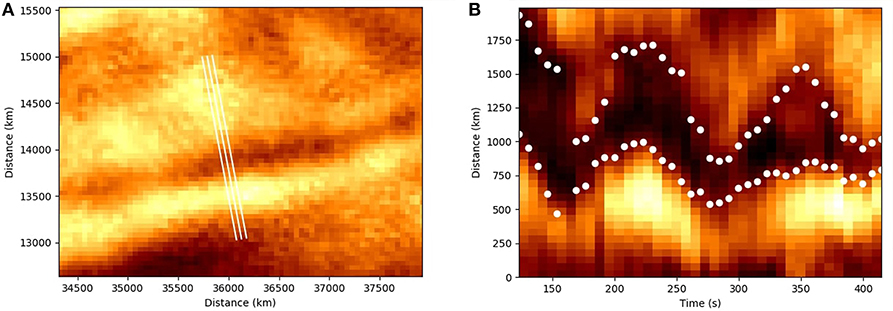
Figure 5. (A) A typical example of a ROSA Hα fibril taken at t = 399.36 s from the start of the observational window. The middle slit is placed perpendicular to the fibril. The mean of the intensities along the middle slit and two parallel slits at a pixel each side at each time step is plotted in (B). The white dots correspond to the boundaries of the fibril, calculated as the position of half-maximum of the fitted Gaussian. Axis values are in units from the bottom left of the observational domain.
To find the boundaries of the fibrils so that the boundary oscillation amplitudes can be determined, we fit a Gaussian function to each time frame of the time-distance data (Figure 5B). The boundaries are taken to be the positions along the slit at which the fitted Gaussian reaches half-maximum. Due to the limited number of data-points across each fibril, the high signal-to-noise ratio, and to improve the fitting stability, for time frames when the Gaussian fitting failed, the fitting domain was reduced to 10 pixels either side of the boundaries on the previous time step.
Fibrils for which the stabilized Gaussian fitting failed on a significant proportion of time steps were omitted from the analysis. The boundaries were cross-checked and the small number of isolated anomalous points were smoothed over using a linear interpolation between the preceding and following time frames. The width of each fibril was taken as the mean distance between the boundaries throughout the time window for which the stabilized Gaussian fitting was successful.
4.1.4. Frequency and Amplitude Measurement
For each fibril, both sets of boundary data were then detrended with a cubic polynomial fit by least-squares regression. The detrended boundaries were then fit with a sinusoidal curve (Figure 6) due to there being too few data points to make wavelet analysis useful. The frequency of each wave is taken to be the average of the frequencies of both boundary sinusoids. The amplitude ratio is the signed ratio of the amplitudes of the boundary sinusoids.
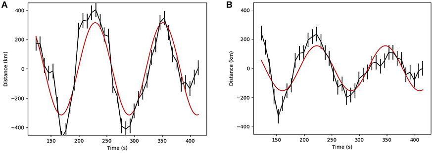
Figure 6. (A) Top and (B) bottom boundary positions along the averaged slits given in Figure 5A (black line), detrended with a cubic polynomial. The error bounds on each point are the pixel size and therefore correspond to the error in the observations rather than the error in the trend fitting so represent a lower bound on the total error. The boundaries are fitted with a sinusoid (red line).
4.1.5. Phase Speed Measurement
For each fibril, we plotted the cross-sectional width variation through time at five parallel slits, each five pixels apart and perpendicular the fibril. The widths at each time-step were calculated as the position of the half-maximum of the fitted Gaussian function along each slit. The intensity along each of the five slits used for the phase speed measurement is the mean of the intensities across three parallel slits spaced a pixel apart, as described in section 4.1.3. The width variation was smoothed with a 3-point box-car function and the temporal lag in the smoothed width variation was fitted with a straight line (see Figure 7). The gradient of this line is the estimated phase speed.
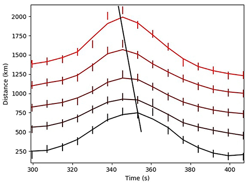
Figure 7. Five parallel slits, spaced by five pixels, are placed perpendicular to each fibril. The widths, calculated from the fitted Gaussian along each slit, are plotted and displaced in the y-direction by five pixels = 250 km, the distance between each slit. The peaks and troughs of the width oscillations are fitted by a straight line, the gradient of which is approximately the phase speed.
The measured phase speeds assume that the fibril waveguides are parallel to the plane-of-sky (PoS). In reality, the waveguides are inclined at some angle θ to the PoS. Therefore, the true phase speed will be a factor of sec(θ) greater than the measured phase speed. Unfortunately, using the given data it is impossible to infer the angle θ. The best we can do is use the fact that the fibrils tend to track the magnetic field of the magnetic canopy, which is dominated by a horizontal magnetic field, to motivate the assumption that θ is small. Under this assumption, we can take sec(θ) ≈ 1, to leading order, from which it follows that the true phase speed is approximately equal to the measured phase speed in the observational plane.
Additionally, it might appear that we have assumed that the oscillations are approximately polarized in the PoS because the amplitudes are measured in the observational plane. However, the amplitudes only enter the inversion calculation as a ratio, therefore eliminating any projection effects anyway.
4.1.6. Inversion Procedure
Using the results from section 4.1.2, we employed a numerical inversion procedure to estimate the Alfvén speed within the fibrils (more information can be found in Allcock and Erdélyi, 2018). First, for each fibril oscillation, the mode of oscillation (quasi-sausage or quasi-kink) was determined by assessment of the phase-shift between the oscillations on each boundary. After prescribing all the parameters apart from the internal Alfvén speed, vA1, in Equations (4.2) or (4.3) (depending on the mode identified), the secant method was used to find the Alfvén speed estimation.
For each inversion, we specified an internal sound speed of c0 = 10 km s−1 and density ratios of ρ1/ρ0 = 0.1 and ρ2/ρ0 = 0.2, and vice versa depending on which side had the largest amplitude. In the absence of any density-sensitive proxies from the data, they were chosen to match the order of magnitude difference between the densities external and internal to the fibrils as expected from previous fibril observations (Leenaarts et al., 2012; Morton et al., 2012).
To reduce the chance of finding the wrong root when the inverse problem is multi-valued, a hundred initial values for vA evenly spaced between 1 and 200 km s−1 were tried and only fibrils for which the inversion produced the same value for almost all of the initial values were included in the results.
4.1.7. Results
We made a successful inversion of five chromospheric fibrils and recorded the parameters in Table 2. Two of the fibrils were identified as oscillating in the quasi-kink mode and three in the quasi-sausage mode. All of the identified MHD modes are expected to be fast modes due to their phase speeds exceeding the expected sound speed. Fibril 1 exhibited a change in direction of propagation before breaking up. The other fibril oscillations propagated in one direction for the duration of the time for which Gaussian fitting was successful. The inverted Alfvén speeds agree with expected values for chromospheric fibrils (Morton et al., 2012). Although, we acknowledge the high degree of uncertainty in present and previous chromospheric Alfvén speed estimates.
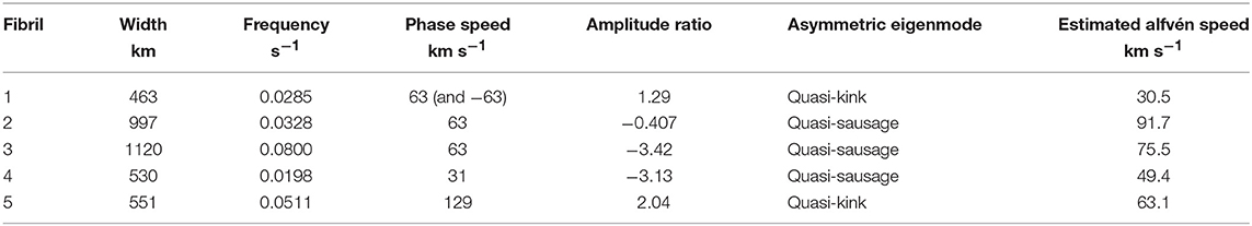
Table 2. A table of measured parameters, identified mode, and estimated local Alfvén speed of five chromospheric fibrils.
The error in the inversions due to the input parameters comes mainly from the density ratios. In Allcock and Erdélyi (2018), we determined that the relative errors in the density ratios are reduced by a factor of two when propagated into the errors in the inverted Alfvén speed. However, this was calculated by using an analytical inversion procedure, which involved taking a further approximation of the model. In the present work, we have used a numerical inversion procedure to avoid having to make such an approximation. To determine how the density errors propagate through the numerical inversion implemented here, we ran the inversion for a range of density parameters. We found that the relative error in each density ratio is approximately halved after propagating through the numerical inversion. As an example, for fibril 1, an input density ratio of ρ2/ρ0 = 0.4 rather than 0.2, i.e., a 100% difference, leads to an Alfvén speed estimate of 44.8 km s−1, approximately 50% greater than the 30.5 km s−1 estimated using ρ2/ρ0 = 0.2.
4.2. High-Beta Asymmetric Slab Eigenmodes
The dispersion relations of each slab configuration provide us with a wide variety of normal solutions. Since a completely general analytical description of all these waves does not seem possible, it is a worthwhile endeavor to further study the various solutions and uncover certain fundamental analytical relationships between the relevant parameters, next to, of course, applying the above-mentioned numerical inversion schemes.
One possible avenue is to examine how the ratios of plasma and magnetic pressures in all the domains influence the existence and properties of the different types of normal modes. This ratio is described by the plasma-β parameter, defined as βj = pj/pj,m for a domain j, where pj is the plasma pressure and pj,m is the magnetic pressure in the given domain.
As the solar atmosphere shows a range of complex and fine magnetic structures, we have chosen the externally magnetic asymmetric slab model to provide an example of the theoretical side of the investigation. Furthermore, since we have primarily focused on lower solar atmospheric applications, we will limit this section to the discussion of high-β asymmetric slab systems.
For the case when Λ2 is of the same order as Λ0, it is possible to derive an approximate decoupled dispersion relation, which is given by
Unlike the full dispersion relation (Equation 3.7), this relation, applicable to the special case of weak asymmetry, decouples into a separate equation for quasi-sausage (tanh version) and quasi-kink (coth version) eigenmodes, which is analogous to the decoupling of the symmetric case detailed in Edwin and Roberts (1982). In the infinite-β limit, magnetic forces are negligible compared to the pressure gradient force, i.e., cj/vAj ≫ 1, for j = 0, 1, 2. In this scenario, only essentially purely acoustic body waves occur. If we take into account that the total pressure must balance across the boundaries, and that the pressure in this case is purely the kinetic pressure, the dispersion relation (Equation 4.4) can be reduced to
where
and is a modified wavenumber coefficient introduced in the description of body waves (see e.g., Edwin and Roberts, 1982). For trapped body waves to exist, the conditions n1z, m0z and m2z > 0 must be fulfilled. This necessitates that the angular frequency of the waves should satisfy . The band of fast body waves therefore exists in the phase speed interval between the internal sound speed and the lower of the two external ones. Due to the periodicity of the tangent and cotangent functions, an infinite number of harmonics exist in the direction of structuring. Introducing the notation cm = min(c0, c2), the waves are expected to behave as . By using the general method of describing body waves irrespective of plasma-β value (see e.g., Roberts, 1981a; Allcock and Erdélyi, 2017), the coefficients νj can be determined. This leads to the following expression for the quasi-sausage mode solutions:
The approximation for quasi-kink modes becomes
A basic diagnostic purpose may be fulfilled by making these approximations. Namely, Equations (4.7) and (4.8) showcase a simple connection between the lower external sound speed, and the ratio of the same side's external density to the internal one for any given value of the wavenumber and angular frequency of a given order body mode. Thus, knowledge of one of these parameters can provide an estimate of the other.
In accordance with our analytical expectations, seeking numerical solutions in a few interesting high-β configurations reveals that, while a few types of eigenmodes will not occur in high-β slab systems, we can still hope to detect several types of waves in lower solar atmospheric conditions. For example, Figure 8A illustrates the results of the numerical examination in a typical high-β equilibrium configuration. There is a band of fast body modes confined between the sound speeds and a band of slow body modes between the internal Alfvén and cusp speeds. Here, slow surface waves are present as well, which would not occur in the low-β limit (corresponding more closely to higher atmospheric conditions).
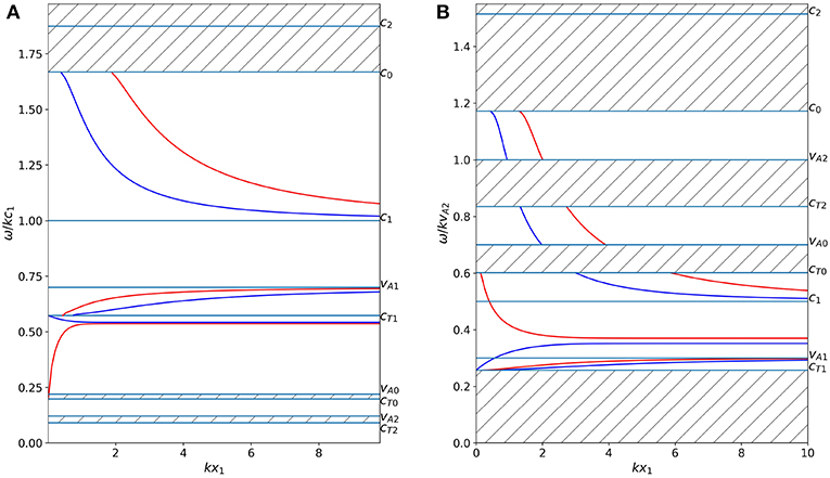
Figure 8. Solutions to the dispersion relation for high-β cases. (A) Slow and fast mode body waves, as well as slow surface waves are present when vA1 = 0.7c1, vA0 = 0.2c1, vA2 = 0.1c1, c0 = 1.6683c1, c2 = 1.8742c1, ρ0/ρ1 = 0.5, ρ2/ρ1 = 0.4. (B) Three bands of fast body modes, one band of slow body modes, and a pair of slow surface modes exist when vA1 = 0.2vA2, vA0 = 0.7vA2, c1 = 0.5vA2, c0 = 1.1vA2, c2 = 1.8vA2, ρ0/ρ1 = 0.2008, ρ2/ρ1 = 0.1163. In each panel, only a couple of examples in each band of body modes are displayed. Blue (red) curves illustrate quasi-sausage (quasi-kink) modes. No trapped oscillations exist in the hatched regions.
Since the magnetic pressure is negligible compared to the plasma pressure in the high-β limit, the possible eigenmodes would not change qualitatively if the relative magnitudes of the external and internal Alfvén speeds were interchanged. On the contrary, if the internal sound speed were greater than the external ones (c1 > c0, c2), no fast waves (neither body, nor surface) could be expected in the system, only slow surface and body waves.
Additionally, Figure 8B illustrates an exciting characteristic not just of high-β systems, but of asymmetric slab systems in general. In this diagnostic diagram, we find slow body modes (cT1 < vph < vA1) and slow surface modes (vA1 < vph < c1) in the region of lower phase speeds. Interestingly, the slow surface quasi-kink mode starts out in the band of fast body modes for thin slabs (small kx1), while the slow surface quasi-sausage mode begins as a slow body mode. Both of them change character as they progress toward wider slabs (kx1 increases). Additionally, the region of trapped fast body modes is split into three narrower bands (c1 < vph < cT0, vA0 < vph < cT2, and vA2 < vph < c0). This is due to the fact that the asymmetry introduces new cut-off frequencies for the dispersion curves, potentially excluding significant phase speed intervals from the regime of trapped oscillations.
5. Asymmetric Non-stationary Waveguides
So far, we have considered one-slab and multi-slab systems filled with static plasma. However, the study of waveguides incorporating steady flows has also been an important aspect of solar atmospheric research (see e.g., Nakariakov and Roberts, 1995; Terra-Homem et al., 2003). The inclusion of flows in our models modifies the phase speeds and cut-off speeds of the observable modes, and it opens up the possibility for the Kelvin-Helmholtz instability (KHI) to appear in the system. In order to showcase some of these meaningful physical additions to the behavior of perturbations in our MHD waveguides, in this section we will analyse MHD wave propagation in a few non-stationary slab systems that characterize solar waveguides with bulk flows present.
5.1. General Non-stationary Slab
The complex and dynamic solar atmosphere is observed to contain plasma flows and instances of Kelvin-Helmholtz Instability (KHI) throughout (e.g., Ryutova et al., 2010; Ofman and Thompson, 2011; Zhelyazkov, 2015). In the light of these detections, we can further extend the applicability of our slab models if we lift the restriction of static plasma, and allow for the presence of background bulk flow motions in one or several domains in the equilibrium.
Let us therefore consider a new one-slab model that incorporates asymmetric plasma with magnetic fields and steady flows. The slab is bounded by two interfaces at ±x1. Both the slab and the semi-infinite domains that enclose it are filled with uniform, compressible, inviscid plasma of different density, ρ, pressure, p, and temperature, T. Each part of the system is permeated by vertical magnetic fields, , of different strength, and is subject to steady flows in the vertical direction, , of different speeds:
where Fj denotes any of the five physical scalar parameters listed above, namely Fj = constant, for j = 0, 1, 2 (Figure 9).
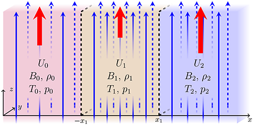
Figure 9. The equilibrium configuration for a steady and magnetized slab embedded in a steady, magnetized, and asymmeric semi-infinite plasma. The notation is the same as in the previous figures, with the addition of the thick red arrows representing the vertical plasma flow, .
We assume, as before, that perturbations within the system are governed by the ideal MHD equations (Equations 2.1). This time, we linearize these in the presence of Uj equilibrium steady flows, and then we perform Fourier-analysis, seeking plane wave solutions that propagate along the slab. Thus, a governing equation is obtained for each domain, which is formally similar to the case of the stationary slab systems:
where
Due to the presence of a steady background flow, however, instead of the angular frequency, ω, it is the Doppler-shifted frequency, defined as
that appears in all the coefficients.
Physically realistic trapped wave solutions still have to be evanescent far away from the slab (as x → ±∞), and uphold the continuity of the total pressure perturbation and the Lagrangian displacement across the slab boundaries. In order to find a non-trivial solution for the system of equations formulated by these boundary conditions, we have to solve
where
Written in terms of the characteristic speeds, the dispersion relation, Equation (5.5), of the general steady asymmetric slab system, takes the following form:
This relation is formally analogous to Equation (3.7) governing the static asymmetric slab system in a magnetic environment. Here, however, flows are present in all the domains, therefore, the Doppler-shifted frequencies take the place of the “ordinary” angular frequency in every expression.
Furthermore, just like in the case of the static asymmetric slab system, an approximate, decoupled dispersion relation can be obtained if conditions are different, but closely similar on the two sides of the slab:
For any unspecified measure of asymmetry, though, we have to note that (similarly to the stationary case) the dispersion relation of the asymmetric slab system does not decouple into separate equations for traditional (i.e., symmetric) sausage and kink modes, but instead, remains as one expression describing both quasi-sausage and quasi-kink modes. We can therefore say that in the most general description of a uniform, asymmetric one-slab system, the eigenmodes will reflect the differences between the external parameters on either side of the slab and possess mixed characteristics of the traditional (symmetric) sausage and kink mode oscillations.
5.2. Steady Slab in an Asymmetric Non-magnetic Environment
A special case of the general steady one-slab model has been studied by Barbulescu and Erdélyi (2018), whose results are summarized and adapted to our notation in the following subsection. They analyzed the propagation of magnetoacoustic waves and the threshold for the KHI in a magnetic slab under the effect of a steady flow, which was enclosed in an asymmetric, non-magnetic environment filled with stationary plasma (Figure 10). They derived the full dispersion relation of this configuration, which, in our notation, becomes
where
Equation (5.9) can be obtained as a special case of Equation (5.7) by setting the external magnetic fields and flows to B0 = B2 = U0 = U2 = 0.
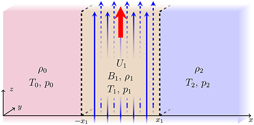
Figure 10. The equilibrium configuration for a steady and magnetized slab in an asymmetric non-magnetic environment.
In the presence of internal or external flows, it is worthwhile to extend the investigation of eigenmodes to negative phase speeds as well, since the symmetry between forward- and backward-propagating modes that characterizes stationary slabs, becomes broken in the presence of a steady state. Barbulescu and Erdélyi (2018) demonstrated that a strong enough internal flow is able to shift backward propagating modes into forward propagating ones. The presence of external asymmetry does not influence this phenomenon; instead, it manifests through the introduction of new, additional cut-off frequencies for trapped oscillations. Furthermore, any deviation from symmetry of the parameters in the external plasma regions leads to a greater range of slab widths (kx1) for which the system is KH unstable.
An exciting application of this model can be found, e.g., in the form of KHI detected at the flank of a coronal mass ejection (CME). Based on observations of Foullon et al. (2011), made using the Atmospheric Imaging Assembly on board the Solar Dynamics Observatory on November 3, 2010, Barbulescu and Erdélyi (2018) modeled the structure made up of the CME core, the CME flank, and the lower-density solar corona as a non-stationary slab enclosed between two static regions. They interpreted the observations as a slow kink mode and, by finding numerical solutions to the dispersion relation that agreed with the observed values, provided an estimate for the density of the CME ejecta.
The authors noted, however, that a limitation on the validity of this result stems from the inability of the model to explain why the KHI was not observed between the CME core and flank regions. A further approximation they made was that they considered the CME core to be static, since on the timescale of the KHI, the flow in that region is much slower than on the flank (Barbulescu and Erdélyi, 2018). Considering these simplifications, it might be advantageous to use a more complex model that includes external magnetic fields everywhere, as well as flows in the external domains, such that will be described in the following section.
5.3. Steady Slab in an Asymmetric Magnetic Environment With Bulk Flows
An interesting generalization of the steady slab problem, which offers some analytical simplification and reduces the number of parameters needed for a possible inversion from observational data, but still keeps the broad applicability of the model, is a configuration in which different magnetic fields permeate all parts of the asymmetric slab system, while only the internal plasma is stationary (Figure 11). For such a model, the dispersion relation (Equation 5.7) reduces to
with
The decoupled dispersion relation also takes a simpler form:
Of particular interest is once again the case when the system is filled with high-β plasma in each region, which is representative of the conditions in the lower atmospheric layers of our Sun. In order to better demonstrate the effect that the bulk flows have on the permitted modes, we can convert the previous two-flow system into a configuration containing one internal and one external flow by changing the frame of reference. Now U2,new = 0, U1,new = −U2,old, and U0,new = U0,old − U2,old. In the analytically tractable approximation of infinite-β, to describe fast body modes, Equation (5.13) in the new frame of reference simply becomes
where . The analytical description of the expected backward- and forward-propagating fast body waves, in this case, becomes
for quasi-sausage modes, and
for quasi-kink modes. The equilibrium bulk flow directly affects the phase speed of the guided waves, as it can be seen. Further numerical evaluations reveal that both the internal and external flow speeds can significantly change the angular frequency of the supported modes and influence the magnitudes of cut-off frequencies.
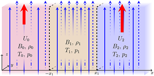
Figure 11. The equilibrium configuration for a slab with two external flows.
Although it is possible to convert such a configuration into an analytically more advantageous one, due to the initial asymmetry between the steady and static regions, new, unique variations arise in this configuration, which cannot be made symmetric or fully externally stationary simply by a change in the frame of reference, like it was possible in the case of a symmetric plasma environment described by Nakariakov and Roberts (1995).
A prime candidate for applying the high-beta two-flow slab model can be found in magnetic bright points in the solar photosphere. These small concentrations of intense magnetic field are wedged into the dark inter-granular lanes. Often, MBPs display an elongated shape (Liu et al., 2018), which makes it possible to treat them as asymmetric magnetic slabs (for the details and limitations of this approach, see Zsámberger et al., 2018). Let us now consider an isolated MBP enclosed in-between two segments of an inter-granular lane, which will serve as the asymmetric environment, as illustrated by Figure 12. Since the sound speed in the photosphere is around 7 km/s (Hurlburt et al., 2002), we will assume c0 = 7 km s−1 and c2 = 8 km s−1 to demonstrate our point. Following Keys et al. (2013), we set the internal sound speed to c1 = 12 km s−1, and choose the internal Alfvén speed as vA1 = 10 km s−1. Taking into consideration that the magnetic field is significantly weaker outside a bright point, we assume external Alfvén speeds of vA0 = 2.05 km s−1 and vA2 = 3 km s−1. We note that the actual values chosen are estimates and serve to demonstrate how asymmetry is relevant to wave propagation or to the formation of the KHI threshold. To apply our model, we consider the equilibrium bulk flow speed inside the slab to be negligible (U1 = 0 km s−1), and set the other two to values that we could realistically expect in the downflows of intergranular lanes (see Briand and Solanki 1998; Socas-Navarro et al. 2004; Danilovic et al. 2010): U0 = −2 km s−1, U1 = −8 km s−1 (where the negative signs correspond to downflows, while positive values would quantify upflows). The resulting wave solutions to the dispersion relation can be seen in Figure 13.
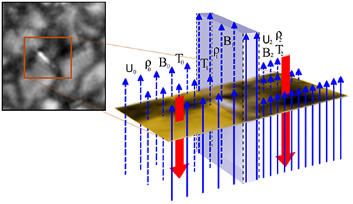
Figure 12. An elongated magnetic bright point visualized as a non-stationary slab. The sketch is based on Figure 12 of Liu et al. (2018), showing TiO 7058 Å observations taken by the New Vacuum Solar Telescope, and a further development on the model featured in Zsámberger et al. (2018). Blue arrows represent the magnetic field lines, and red arrows represent flowing plasma.
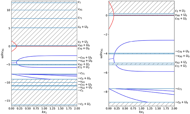
Figure 13. Solutions to the dispersion relation for a high-β MBP. The diagram on the left displays the full range of characteristic speeds, while for the one on the right, the narrower band of interest is enlarged. While in the static case, the characteristic speeds delineate the cut-off frequencies, in a steady slab, these have to be modified by the flow speeds.
For this particular parameter set, only slow mode solutions exist. While in the static case, the characteristic speeds delineate the cut-off frequencies, in a steady slab, these have to be modified by the flow speeds, which makes the propagation of not only slow surface modes (as in the static case for the same set of characteristic speeds and densities), but also that of slow body modes (−c0 + U0 < vph < −cT1) possible. In the presence of such high flow speeds, the symmetry between backward- and forward-propagating modes is strongly broken, as Figure 13 illustrates. This diagnostic diagram contains the real parts of the solutions colored blue, and the imaginary parts (of the surface modes) colored red, in order to let us discern stable and unstable modes. Namely, only the latter possess a non-zero imaginary component, which corresponds to an amplitude growth factor (Barbulescu and Erdélyi, 2018). In the case of the model MBP that we use here to demonstrate the permitted solutions of the dispersion relation, the surface mode solutions (having phase speeds in the range −cT1 < vph < cT0 + U0) are subject to KHI easily (see the dashed part of the blue curve in Figure 13) if the slab is thin. In a wide slab, on the other hand, the wave perturbations can be stable (continuous blue curves), but they do not exist as trapped oscillations for every value of the dimensionless slab width (kx1): in the hatched regions, only leaky modes are found. The solutions would not become unstable for any value of kx1 if the slab was symmetric and the flow speeds did not exceed the internal Alfvén speed. Due to the introduction of the asymmetry, however, the KHI-threshold is lowered, and the instability can set in in this model MBP even though both of the external flow speeds are sub-Alfvénic.
A further application of the asymmetric slab configuration containing two (or even three) different flows can be found in the alternating spine-intraspine pattern of the fibrillar structure in the penumbrae of sunspots, which is closely connected to the Evershed-flow (Tsiropoula, 2000; Borrero and Ichimoto, 2011). Besides the solar atmosphere, the triad of the Earth's magnetopause, magnetosheath, and bow shock region can also be locally considered as a slab-like structure that incorporates varying flows and magnetic fields (Turkakin et al., 2013). Since the asymmetry in the system enables the KHI to develop for a wide range of parameters (Barbulescu and Erdélyi, 2018), this model can also offer a possible explanation of the observed instability in both of these locations.
6. Conclusions
The propagation of linear MHD waves in a multi-layered magnetized plasma structure is studied in the Cartesian slab geometry approximation. Each magnetic slab is uniform and non-stratified (i.e., neither density nor magnetic stratification is considered). A general dispersion relation is derived for a mathematical model of this plasma structured by an arbitrary number of interfaces and two special cases of a plasma slab embedded in an asymmetric non-magnetic and magnetic environment are considered. Unlike the symmetric case, the obtained dispersion relation does not decouple into two dispersion relations of independent wave mode solutions. This coupling manifests as mixed properties of the eigenmodes, which are referred to as quasi-kink and quasi-sausage wave solutions to the governing linear magneto-acoustic equations. These newly obtained eigenmodes are generalizations of the traditionally known sausage and kink modes of symmetric linear MHD waveguides (Table 1).
The asymmetry of waveguides, which is highly likely in many solar structures due to the structural inhomogeneity of the various observed MHD waveguides in the solar atmosphere, is a proxy for background parameters of the waveguide. Motivated by this idea, the Amplitude Ratio Method from Allcock and Erdélyi (2018) is employed, as a proof of concept, to estimate the local Alfvén speed in five chromospheric fibrils using Hα data from the ROSA imager. We find that many of the observed fibrils displayed asymmetric oscillatory behavior, which we interpret here as quasi-kink and quasi-sausage eigenmodes, depending on the phase relationship between the boundary oscillations. The estimates of the local Alfvén speed, obtained after inverting the observed information, agree with highly uncertain expected values from photospheric extrapolations.
Incorporating asymmetric external magnetic fields into the slab model provides a further useful middle-ground between the breadth of applications and analytical tractability. From coronal hole boundaries, through prominences, to MBPs of the photosphere, a variety of solar atmospheric fine structures can be more closely described as a magnetized asymmetric slab system. Next to numerical root-finding methods, making certain well-known approximations, such as investigating the limit of a thin or a wide slab, low or high values of the plasma-β, allows us to concisely describe the various quasi-sausage, quasi-kink, surface, or body modes that we expect, and to identify some of their fundamental characteristics.
A further step in generalizing the newly developed asymmetric slab models is to move away from stationary plasmas, and incorporate equilibrium bulk flows (i.e., steady states) in one or more regions. This generalization has the consequence that the angular frequencies are replaced by their Doppler-shifted counterparts in the dispersion relations, and the cut-off frequencies for the different eigenmodes are influenced by the magnitudes of the flows. An externally stationary asymmetric slab system serves as a reasonable approximation of CME flank regions. Including multiple external bulk flows widens the scope of applicability to e.g., MBPs residing between sections of different inter-granular flows, fibrils in the dynamic sunspot penumbra, and the magnetosheath region of Earth's magnetosphere. Therefore, for all these features, such a slab configuration can offer a reasonable initial model that explains the observed KHI.
The one- or multi-slab approach to asymmetric waveguides has wide applicability in different layers of the solar atmosphere. MHD waves have been observed in many structures of our Sun, and to correctly interpret some of them, the asymmetry of their environments should be taken into account.
A variety of waves have been observed in sunspot structures, for example, in the penumbra, which itself shows a filamentary structure. Neighboring filaments may be modeled by different plasma and magnetic parameters, and they have been observed to support upward propagating slow-mode magneto-acoustic waves in the form of running penumbral waves (Bloomfield et al., 2007; Freij et al., 2014; Löhner-Böttcher and Bello González, 2015). The multi-slab model may be a good approximation for high-frequency waves. Another sunspot element where asymmetry of the plasma environment could heavily influence wave propagation is the light bridge and corresponding light wall reaching up into higher layers of the atmosphere, which are trapped between two, sometimes vastly different umbral cores. Oscillations recently detected in light walls have been interpreted as signatures of propagating magneto-acoustic (shock) waves (Yang et al., 2015; Zhang et al., 2017).
Small, bright magnetic flux concentrations are located in the intergranular lanes wedged in-between two granular cells, whose plasma and magnetic properties can potentially be highly different. This asymmetry then naturally affects the characteristics of any waves present in the above-mentioned MBPs. These small-scale magnetic elements, which might take on the appearance of a nearly circular flux tube or a strongly elongated slab-like structure, have been put forward as the photospheric anchor points of chromospheric waveguides that show sausage-mode oscillations (Morton et al., 2012). The existence of a wealth of magneto-acoustic oscillations within MBPs themselves has also been concluded from high-cadence observations performed at different altitudes (Jess et al., 2012). Chromospheric manifestations of bright points have been confirmed to sway around their photospheric counterparts, signaling the presence of kink type oscillations (Xiong et al., 2017).
In section 4, we have already addressed that chromospheric fibrils exist in a complex, asymmetric environment, and whether they are considered as flux tubes or as magnetic slabs, the asymmetry can lead to the appearance of different-looking modes, for which previously the only explanation was the simultaneous presence of sausage and kink type waves (Morton et al., 2012; Mooroogen et al., 2017). Higher up in the solar atmosphere, MHD waves are also found in prominences (Arregui et al., 2018), which themselves lie between different layers of the vertically stratified corona. Another coronal example of applicability could be the studies of MHD wave propagation at the boundary of coronal holes (see e.g., Banerjee et al., 2000; Banerjee, 2012).
Additionally, Alfvén waves are also known to propagate in the solar atmosphere. However, Alfvén waves are local waves as opposed to the sausage and kink waves that have a global character. Alfvén waves propagate along constant magnetic surfaces. If there is a suitable driver, each magnetic surface supports its own Alfvén wave, which will be characterized by the properties of the individual flux sheets and will not be strongly affected by the rest of the plasma environment. Because of this, Alfvén waves are not very promising disturbances for the application of our magneto-seismological technique described in this paper.
As detailed above, recent high-resolution state-of-the-art ground-based or space-borne observations clearly show that there is strong structuring (inhomogeneity) and dynamics in the observed solar (and magnetospheric) MHD waveguides. Solar MHD wave theory is boosted by the development of solar magneto-seismology; see the avalanche of Space Sci. Reviews since 2010. SMS is an excellent tool to obtain sub-resolution information about MHD waveguides present in the Sun. Here we make a step forward by applying this tool to structured MHD waveguides by demonstrating, as a proof-of-concept in a limited number of test cases, how this newly developed tool can be used for the much wanted solar plasma diagnostics. This latter result has an additional importance, given that the field of solar physics is at the brink of its greatest historic development: the imminent commencing of our 4 m aperture ground-based DKIST telescope.
Data Availability
The datasets for this manuscript are not publicly available because Data can be requested freely directly from the corresponding author. Requests to access the datasets should be directed to cm9iZXJ0dXNAc2hlZmZpZWxkLmFjLnVr.
Author Contributions
The research concept was formulated and the project led by RE. MA derived the results of the asymmetric slab in a non-magnetic environment, including the associated solar magneto-seismology theory, and application to observations. DS derived the results of the general multi-layered waveguide. NZ derived the results of the asymmetric slab in a magnetic environment and the generalizations to flowing plasma, and prepared the sample parametric solutions presented.
Conflict of Interest Statement
The authors declare that the research was conducted in the absence of any commercial or financial relationships that could be construed as a potential conflict of interest.
The handling editor declared a past co-authorship with one of the authors RE.
Acknowledgments
MA acknowledges support from the University Prize Scholarship awarded by the University of Sheffield. DS acknowledges support from the University of Sheffield. NZ is grateful for the support of the University of Debrecen and the University of Sheffield. RE is grateful to Science and Technology Facilities Council (STFC_grant_nr_ST/M000826/1) UK for the support received. Observations were obtained at the National Solar Observatory, operated by the Association of Universities for Research in Astronomy, Inc. (AURA), under agreement with the National Science Foundation. We would like to thank the technical staff at the DST for their help and support during the observations. Further thanks are required for M. Mathioudakis Francis Keenan (Queen's University Belfast, UK) for ROSA support in 2010 when the observing proposal was awarded and data taken. For the relevant ROSA data discussed in the paper please contact RE, while access to the overall ROSA archive is available via weblink1.
All authors acknowledge the valuable input from M. Barbulescu regarding waves and instabilities in steady plasma and thank him for making available the PyTES software package (https://github.com/BarbulescuMihai/PyTES). The authors are also grateful to F. Allian for use of and assistance with his code for processing the ROSA Hα data.
Footnotes
1. ^https://star.pst.qub.ac.uk/wiki/doku.php/public/research_areas/solar_physics/rosa_reconstructed_archive
References
Allcock, M., and Erdélyi, R. (2017). Magnetohydrodynamic waves in an asymmetric magnetic slab. Solar Phys. 292:35. doi: 10.1007/s11207-017-1054-y
Allcock, M., and Erdélyi, R. (2018). Solar magnetoseismology with magnetoacoustic surface waves in asymmetric magnetic slab waveguides. Astrophys. J. 855:90. doi: 10.3847/1538-4357/aaad0c
Andries, J., van Doorsselaere, T., Roberts, B., Verth, G., Verwichte, E., and Erdélyi, R. (2009). Coronal seismology by means of Kink oscillation overtones. Space Sci. Rev. 149, 3–29. doi: 10.1007/s11214-009-9561-2
Arregui, I., Oliver, R., and Ballester, J. L. (2012). Prominence oscillations. Living Rev. Solar Phys. 9:2. doi: 10.12942/lrsp-2012-2
Arregui, I., Oliver, R., and Ballester, J. L. (2018). Prominence oscillations. Living Rev. Sol. Phys. 15:3. doi: 10.1007/s41116-018-0012-6
Ballai, I., and Ruderman, M. S. (2011). Nonlinear effects in resonant layers in solar and space plasmas. Space Sci. Rev. 158, 421–450. doi: 10.1007/s11214-010-9717-0
Banerjee, D. (2012). “Diagnosing chromosphere- Corona connection by waves in open structures,” in 39th COSPAR Scientific Assembly, Vol. 39 (Mysore), 96.
Banerjee, D., Teriaca, L., Doyle, J. G., and Lemaire, P. (2000). Polar Plumes and Inter-plume regions as observed by SUMER on SOHO. Solar Phys. 194, 43–58. doi: 10.1023/A:1005253413687
Barbulescu, M., and Erdélyi, R. (2018). Magnetoacoustic waves and the Kelvin-Helmholtz instability in a steady asymmetric slab. I: the effects of varying density ratios. Solar Phys. 293:86. doi: 10.1007/s11207-018-1305-6
Berger, T. E., and Title, A. M. (1996). On the dynamics of small-scale solar magnetic elements. Astrophys. J. 463:365. doi: 10.1086/177250
Bloomfield, D. S., Lagg, A., and Solanki, S. K. (2007). The nature of running penumbral waves revealed. Astrophys. J. 671, 1005–1012. doi: 10.1086/523266
Borrero, J. M., and Ichimoto, K. (2011). Magnetic structure of sunspots. Living Rev. Sol. Phys. 8:4. doi: 10.12942/lrsp-2011-4
Briand, C., and Solanki, S. K. (1998). Velocity fields below the magnetic canopy of solar flux tubes: evidence for high-speed downflows? Astron. Astrophys. 330, 1160–1168.
Danilovic, S., Schüssler, M., and Solanki, S. K. (2010). Magnetic field intensification: comparison of 3D MHD simulations with Hinode/SP results. Astron. Astrophys. 509:A76. doi: 10.1051/0004-6361/200912283
Díaz, A. J., Oliver, R., and Ballester, J. L. (2005). Fast magnetohydrodynamic oscillations in a multifibril Cartesian prominence model. Astron. Astrophys. 440, 1167–1175. doi: 10.1051/0004-6361:20052759
Díaz, A. J., and Roberts, B. (2006). Fast magnetohydrodynamic oscillations in a fibril prominence model. Solar Phys. 236, 111–126. doi: 10.1007/s11207-006-0137-y
Edwin, P. M., and Roberts, B. (1982). Wave propagation in a magnetically structured atmosphere. III - The slab in a magnetic environment. Solar Phys. 76, 239–259. doi: 10.1007/BF00170986
Foullon, C., Verwichte, E., Nakariakov, V. M., Nykyri, K., and Farrugia, C. J. (2011). Magnetic Kelvin-Helmholtz instability at the sun. Astrophys. J. Lett. 729:L8. doi: 10.1088/2041-8205/729/1/L8
Freij, N., Scullion, E. M., Nelson, C. J., Mumford, S., Wedemeyer, S., and Erdélyi, R. (2014). The detection of upwardly propagating waves channeling energy from the chromosphere to the low corona. Astrophys. J. 791:61. doi: 10.1088/0004-637X/791/1/61
Goossens, M., Erdélyi, R., and Ruderman, M. S. (2011). Resonant MHD waves in the solar atmosphere. Space Sci. Rev. 158, 289–338. doi: 10.1007/s11214-010-9702-7
Heyvaerts, J., and Priest, E. R. (1983). Coronal heating by phase-mixed shear Alfven waves. Astron. Astrophys. 117, 220–234.
Hurlburt, N. E., Alexander, D., and Rucklidge, A. M. (2002). Complete models of axisymmetric sunspots: magnetoconvection with coronal heating. Astrophys. J. 577, 993–1005. doi: 10.1086/342154
Jess, D. B., Mathioudakis, M., Christian, D. J., Keenan, F. P., Ryans, R. S. I., and Crockett, P. J. (2010). ROSA: A high-cadence, synchronized multi-camera solar imaging system. Solar Phys. 261, 363–373. doi: 10.1007/s11207-009-9500-0
Jess, D. B., Shelyag, S., Mathioudakis, M., Keys, P. H., Christian, D. J., and Keenan, F. P. (2012). Propagating wave phenomena detected in observations and simulations of the lower solar atmosphere. Astrophys. J. 746:183. doi: 10.1088/0004-637X/746/2/183
Keys, P. H., Mathioudakis, M., Jess, D. B., Shelyag, S., Christian, D. J., and Keenan, F. P. (2013). Tracking magnetic bright point motions through the solar atmosphere. Mon. Not. Roy. Astron. Soc. 428, 3220–3226. doi: 10.1093/mnras/sts268
Leenaarts, J., Carlsson, M., and Rouppe van der Voort, L. (2012). The formation of the Hα line in the solar chromosphere. Astrophys. J. 749:136. doi: 10.1088/0004-637X/749/2/136
Liu, Y., Xiang, Y., Erdélyi, R., Liu, Z., Li, D., Ning, Z., et al. (2018). Studies of isolated and non-isolated photospheric bright points in an active region observed by the new vacuum solar telescope. Astrophys. J. 856:17. doi: 10.3847/1538-4357/aab150
Löhner-Böttcher, J., and Bello González, N. (2015). Signatures of running penumbral waves in sunspot photospheres. Astron. Astrophys. 580:A53. doi: 10.1051/0004-6361/201526230
Luna, M., Terradas, J., Oliver, R., and Ballester, J. L. (2006). Fast magnetohydrodynamic waves in a two-slab coronal structure: collective behaviour. Astron. Astrophys. 457, 1071–1079. doi: 10.1051/0004-6361:20065227
Mathioudakis, M., Jess, D. B., and Erdélyi, R. (2013). Alfvén waves in the solar atmosphere. From theory to observations. Space Sci. Rev. 175, 1–27. doi: 10.1007/s11214-012-9944-7
Mooroogen, K., Morton, R. J., and Henriques, V. (2017). Dynamics of internetwork chromospheric fibrils: basic properties and magnetohydrodynamic kink waves. Astron. Astrophys. 607:A46. doi: 10.1051/0004-6361/201730926
Morton, R. J., Verth, G., Jess, D. B., Kuridze, D., Ruderman, M. S., Mathioudakis, M., et al. (2012). Observations of ubiquitous compressive waves in the Sun's chromosphere. Nat. Commun. 3:1315. doi: 10.1038/ncomms2324
Nakariakov, V. M., and Roberts, B. (1995). Magnetosonic waves in structured atmospheres with steady flows, I. Solar Phys. 159, 213–228. doi: 10.1007/BF00686530
Ofman, L., and Thompson, B. J. (2011). SDO/AIA observation of Kelvin-Helmholtz instability in the solar corona. Astrophys. J. Lett. 734:L11. doi: 10.1088/2041-8205/734/1/L11
Roberts, B. (1981a). Wave propagation in a magnetically structured atmosphere - II - waves in a magnetic slab. Solar Phys. 69, 39–56. doi: 10.1007/BF00151254
Roberts, B. (1981b). Wave propagation in a magnetically structured atmosphere. I - surface waves at a magnetic interface. Solar Phys. 69, 27–38. doi: 10.1007/BF00151253
Roberts, B., Edwin, P. M., and Benz, A. O. (1984). On coronal oscillations. Astrophys. J. 279, 857–865. doi: 10.1086/161956
Ruderman, M. S. (1992). Soliton propagation on multiple-interface magnetic structures. J. Geophys. Res. 97:16. doi: 10.1029/91JA02672
Ruderman, M. S., and Erdélyi, R. (2009). Transverse oscillations of coronal loops. Space Sci. Rev. 149, 199–228. doi: 10.1007/s11214-009-9535-4
Ryutova, M., Berger, T., Frank, Z., Tarbell, T., and Title, A. (2010). Observation of plasma instabilities in quiescent prominences. Solar Phys. 267, 75–94. doi: 10.1007/s11207-010-9638-9
Shukhobodskaia, D., and Erdélyi, R. (2018). Propagation of surface magnetohydrodynamic waves in asymmetric multilayered plasma. Astrophys. J. 868:128. doi: 10.3847/1538-4357/aae83c
Socas-Navarro, H., Martínez Pillet, V., and Lites, B. W. (2004). Magnetic properties of the solar internetwork. Astrophys. J. 611, 1139–1148. doi: 10.1086/422379
Terra-Homem, M., Erdélyi, R., and Ballai, I. (2003). Linear and non-linear MHD wave propagation in steady-state magnetic cylinders. Solar Phys. 217, 199–223. doi: 10.1023/B:SOLA.0000006901.22169.59
Tsiropoula, G. (2000). Physical parameters and flows along chromospheric penumbral fibrils. Astron. Astrophys. 357, 735–742. Available online at: https://ui.adsabs.harvard.edu/abs/2000A&A…357.735T
Turkakin, H., Rankin, R., and Mann, I. R. (2013). Primary and secondary compressible kelvin-helmholtz surface wave instabilities on the earth's magnetopause. J. Geophys. Res. 118, 4161–4175. doi: 10.1002/jgra.50394
van Ballegooijen, A. A., Asgari-Targhi, M., Cranmer, S. R., and DeLuca, E. E. (2011). Heating of the solar chromosphere and corona by Alfvén wave turbulence. Astrophys. J. 736:3. doi: 10.1088/0004-637X/736/1/3
Wiegelmann, T., Thalmann, J. K., and Solanki, S. K. (2014). The magnetic field in the solar atmosphere. Astron. Astrophys. Rev. 22:78. doi: 10.1007/s00159-014-0078-7
Xiong, J., Yang, Y., Jin, C., Ji, K., Feng, S., Wang, F., et al. (2017). The characteristics of thin magnetic flux tubes in the lower solar atmosphere observed by hinode/SOT in the G band and in Ca II H bright points. Astrophys. J. 851:42. doi: 10.3847/1538-4357/aa9a44
Yang, S., Zhang, J., Jiang, F., and Xiang, Y. (2015). Oscillating light wall above a sunspot light bridge. Astrophys. J. Lett. 804:L27. doi: 10.1088/2041-8205/804/2/L27
Zhang, J., Tian, H., He, J., and Wang, L. (2017). Surge-like oscillations above sunspot light bridges driven by magnetoacoustic shocks. Astrophys. J. 838:2. doi: 10.3847/1538-4357/aa63e8
Zhelyazkov, I. (2015). On modeling the Kelvin-Helmholtz instability in solar atmosphere. J. Astrophys. Astron. 36, 233–254. doi: 10.1007/s12036-015-9332-2
Zsámberger, N. K., Allcock, M., and Erdélyi, R. (2018). Magneto-acoustic waves in a magnetic slab embedded in an asymmetric magnetic environment: the effects of asymmetry. Astrophys. J. 853:136. doi: 10.3847/1538-4357/aa9ffe
A. Appendix
A.1. Boundary Conditions in Matrix Form
We rewrite the boundary conditions (2.10) in the compact matrix form (2.12) with [2n + 2] × [2n + 2] matrix M. The precise form of the matrix with the first row corresponding to the continuity of the velocity at x = x0, is
The second row represents the continuity of the total pressure at x = x0:
The last but one row corresponds to the continuity of the velocity at x = xn:
Finally, the last row represents the continuity of the total pressure at x = xn and is
For 1 ≤ j ≤ n−1, general boundary condition takes the form
For the rest of the values i and j, M[i, j] = 0.
Introducing the notation
and using Equations (A1)–(A5), the matrix in explicit form can be written as:
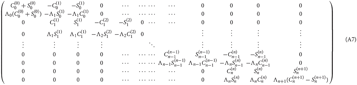
Keywords: solar atmosphere, plasma, waves, magnetohydrodynamics (MHD), magnetic fields, magneto-seismology, fibrils, magnetic bright points
Citation: Allcock M, Shukhobodskaia D, Zsámberger NK and Erdélyi R (2019) Magnetohydrodynamic Waves in Multi-Layered Asymmetric Waveguides: Solar Magneto-Seismology Theory and Application. Front. Astron. Space Sci. 6:48. doi: 10.3389/fspas.2019.00048
Received: 25 February 2019; Accepted: 24 June 2019;
Published: 12 July 2019.
Edited by:
Tom Van Doorsselaere, KU Leuven, BelgiumReviewed by:
Abhishek Kumar Srivastava, Indian Institute of Technology (BHU), IndiaYoura Taroyan, Aberystwyth University, United Kingdom
Inigo Arregui, Instituto de Astrofísica de Canarias, Spain
Copyright © 2019 Allcock, Shukhobodskaia, Zsámberger and Erdélyi. This is an open-access article distributed under the terms of the Creative Commons Attribution License (CC BY). The use, distribution or reproduction in other forums is permitted, provided the original author(s) and the copyright owner(s) are credited and that the original publication in this journal is cited, in accordance with accepted academic practice. No use, distribution or reproduction is permitted which does not comply with these terms.
*Correspondence: Robert Erdélyi, cm9iZXJ0dXNAc2hlZmZpZWxkLmFjLnVr