Multipoint Observations of the June 2012 Interacting Interplanetary Flux Ropes

1. Introduction

Coronal mass ejections (CMEs; e.g., Webb and Howard, 2012) are the key drivers of space weather storms at Earth (e.g., Gosling et al., 1991; Webb et al., 2000; Huttunen et al., 2002; Richardson and Cane, 2012; Kilpua et al., 2017b) and related hazards for many modern technologies and infrastructures in orbit and on the ground (e.g., Schrijver et al., 2015; Eastwood et al., 2017). Particularly geoeffective are those interplanetary CMEs (ICMEs; e.g., Kilpua et al., 2017a) classified as magnetic clouds (e.g., Zhang et al., 2007; Kilpua et al., 2017b). Magnetic clouds are discrete large-scale structures in the solar wind that exhibit enhanced magnetic field magnitudes, coherent rotation of the magnetic field direction over a large angle, and depressed proton temperatures (e.g., Burlaga et al., 1981; Klein and Burlaga, 1982). Magnetic clouds can thus provide the sustained periods of strong and southward magnetic fields in the near-Earth solar wind that are a prerequisite for severe disturbances in the geomagnetic field (e.g., Pulkkinen, 2007). Soon after their discovery, it was suggested that magnetic clouds can be described in terms of cylindrically symmetric force-free magnetic flux ropes (e.g., Goldstein, 1983; Burlaga, 1988). The current consensus holds that magnetic flux ropes are an integral part of all erupting CMEs (e.g., Vourlidas et al., 2013, 2017; Chen, 2017; Green et al., 2018), but are not always detected in interplanetary space due to significant deformations or due to probing of the flux rope far from its center (e.g., Gosling, 1990; Cane et al., 1997; Cane and Richardson, 2003; Huttunen et al., 2005; Jian et al., 2006; Kilpua et al., 2011, 2017a).

Magnetic clouds are often conceptualized as large, curved flux rope loops that extend back to the Sun at both ends, in which the field characteristics and flux rope orientation remain similar over large longitudinal distances (e.g., Burlaga et al., 1990; Crooker et al., 1998; Janvier et al., 2015). Such possible underlying longitudinal coherence is a highly important property both for understanding flux ropes as physical structures in the heliosphere and for forecasting their space weather effects. CME geoeffectiveness depends strongly on the magnetic field magnitude profile and on how the magnetic field vectors vary within the flux rope, i.e., on the “flux rope type” determined by the handedness (chirality) of the field, the axial field direction, and the orientation of the flux rope with respect to the ecliptic plane (e.g., Bothmer and Schwenn, 1998; Huttunen et al., 2005; Kilpua et al., 2017b; Palmerio et al., 2018).

Studies of the spatial and temporal variations of interplanetary flux ropes and their heliospheric interactions are complicated by the lack of suitable multipoint observations. Investigations have mostly taken the form of case studies combining observations from planetary missions (e.g., MESSENGER and Venus Express) and missions located near Earth's orbit (e.g., STEREO and the spacecraft located at L1). For instance, Farrugia et al. (2011), Möstl et al. (2012), and Ruffenach et al. (2012) have all reported significant differences in flux rope properties, in particular in the orientation of flux ropes when the observing spacecraft were separated by a few tens of degrees in heliographic longitude. For weak ICMEs at solar minimum, clear differences have also been reported over longitudinal separations of only a few degrees (e.g., Kilpua et al., 2011). In a recent study, Good et al. (2019) investigated 18 interplanetary flux ropes that were observed by pairs of radially aligned spacecraft in the inner heliosphere (with typical longitudinal separations of ~ 5°) using a technique that maps the magnetic field profile from one spacecraft to the other. Observations matched well at two locations for most cases, but in two cases the tilt of the flux rope differed by more than 20°. In addition, Lugaz et al. (2018) have recently reported clear differences in the magnetic field components of ICME flux ropes at observation points only ~ 0.01 AU apart. These studies imply that flux ropes embedded in CMEs may not be coherent structures on a global-scale, or that significant temporal evolution can occur over relatively short radial distances in the heliosphere (see also discussion in Owens et al., 2017). It should be noted, however, that results derived from flux rope reconstructions may depend strongly on the model used and on boundary time identification, as shown, for example, by Al-Haddad et al. (2013). Multiple CMEs may also interact and merge in interplanetary space, leading to the observation of “complex ejecta” (Burlaga et al., 2002) in which individual characteristics of the flux ropes may no longer be discernible, the preceding flux rope may be compressed (e.g., Liu et al., 2014; Mishra and Srivastava, 2014), or the multiple flux ropes have coalesced into one large structure that resembles a single, coherent flux rope (e.g., Odstrcil et al., 2003; Lugaz et al., 2013, 2017; Chi et al., 2018; Feng et al., 2019).

In this paper, we investigate the interactions, magnetic field structure, and coherence of the interplanetary counterparts of a series of CMEs that erupted from the Sun between June 12 and 14, 2012. The last of these CMEs (June 14 CME) was considerably faster and brighter than the previous two and had a clear Earth-directed component. Observations at Earth's Lagrange L1 point (at 1 AU) show a weak ejecta (June 12 CME) followed by a coherent and strong flux rope structure. This flux rope had the highest magnetic field magnitudes (about 40 nT) measured in the near-Earth solar wind during Solar Cycle 24. Our close inspection of observations reveals that this flux rope was likely composed of the June 13 and June 14 CMEs, which coalesced on their way from Venus to Earth. The Venus Express spacecraft orbiting Venus (at a heliocentric distance of 0.72 AU) also observed the weak June 12 CME, but the June 13 and June 14 CMEs were still separate entities, just on the verge of interaction. As shown in Figure 1, Earth and Venus were almost radially aligned during the passage of the CMEs; their longitudinal separation was 5.4° and their latitudinal separation was 0.2°. The solar and heliospheric characteristics of these CMEs, as well as some of their in-situ signatures (particularly those at Earth), have been investigated in several previous studies (e.g., Kubicka et al., 2016; James et al., 2017, 2018; Palmerio et al., 2017; Srivastava et al., 2018; Pomoell et al., 2019; Scolini et al., 2019; Wang et al., 2019). Here, we focus on comparing interplanetary observations at Venus and Earth. We also discuss how the CMEs are connected with their in-situ counterparts by performing a heliospheric CME propagation simulation and examining heliospheric imagery.

FIGURE 1

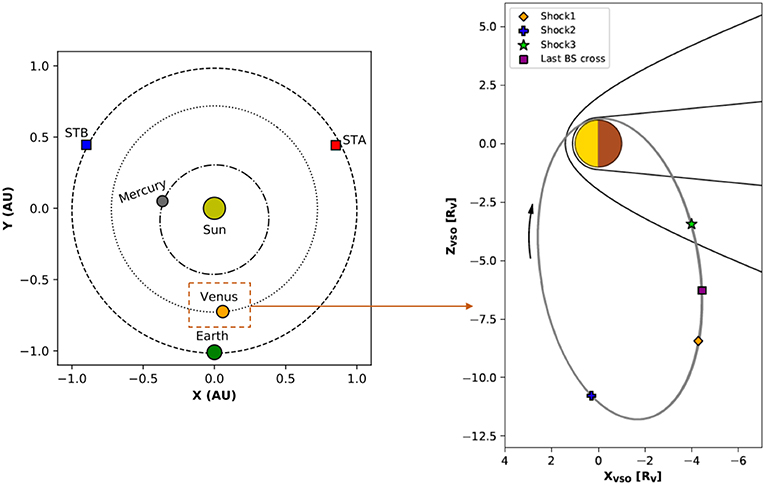
Figure 1. Left: Position of the planets in the inner heliosphere in the ecliptic plane on June 14, 2012. The CME launched on June 14 subsequently arrived at Venus and Earth, which were almost radially aligned at this time. Venus Express (VEX) was orbiting Venus and the Wind and ACE spacecraft were located at the L1 point close to Earth. Right: The orbit of VEX (solid gray line, the orbital direction is indicated by the arrow) around Venus during the time when the June 14 CME reached Venus. The locations of the nominal bow shock (BS) and ion composition boundary (Martinecz et al., 2008) are indicated with black solid lines. Symbols along the orbit indicate the position of VEX during the passage of the interplanetary shocks and the last outbound BS crossing, when VEX entered from the magnetosheath into the solar wind.

The paper is organized as follows: in section 2 we describe the data sets used in this study; in section 3 we present remote-sensing observations of the Sun, the solar corona, and the inner heliosphere, together with in-situ observations at Venus and Earth; this section also includes results from a global heliospheric simulation of the CMEs' propagation; in section 4 we present in-situ flux rope reconstructions; and in section 5 we discuss and summarize our results.

2. Spacecraft Data

Remote-sensing solar disc data used in this study come from the Atmospheric Imaging Assembly (AIA; Lemen et al., 2012) and the Helioseismic and Magnetic Imager (HMI; Schou et al., 2012) instruments onboard the Solar Dynamics Observatory (SDO; Pesnell et al., 2012). AIA provides Extreme Ultra-Violet (EUV) data and HMI provides photospheric vector magnetograms. White-light observations of the solar corona are provided by the COR1 and COR2 coronagraphs, which are part of the Sun Earth Connection Coronal and Heliospheric Investigation (SECCHI; Howard et al., 2008) package onboard the Solar Terrestrial Relations Observatory (STEREO; Kaiser et al., 2008), and by the C2 and C3 coronagraphs of the Large Angle Spectrometric Coronagraph (LASCO; Brueckner et al., 1995) instrument onboard the Solar and Heliospheric Observatory (SOHO; Domingo et al., 1995). The LASCO/C2 field of view extends from 1.5 to 6 solar radii (R_S) and the LASCO/C3 view from 3.7 to 30 R_S. Finally, observations of the inner heliosphere in white light were obtained from the Heliospheric Imager (HI; Eyles et al., 2009) cameras onboard STEREO.

The solar wind data around Venus were obtained from the Venus Express (VEX; Svedhem et al., 2007) spacecraft, which was orbiting Venus at the time of this study. We use magnetic field data from the Magnetometer (MAG; Zhang et al., 2006) instrument and plasma data from the Analyser of Space Plasmas and Energetic Atoms (ASPERA-4; Barabash et al., 2007) instrument. Data from ASPERA-4's Ion Mass Analyser (IMA) and Electron Spectrometer (ELS) sensors have been used. VEX had a 24 h orbit that was highly elliptical and quasi-polar (see Figure 1). It spent a few hours each day within the magnetosheath of Venus. ASPERA-4 was operational at periapsis and apoapsis only, while the magnetometer ran continuously.

Additional in-situ data were obtained from the Wind (Ogilvie and Desch, 1997) and Advanced Composition Explorer (ACE; Stone et al., 1998) spacecraft, which are continuously monitoring the solar wind ahead of Earth at L1. We use magnetic field data from the Magnetic Field Investigation (MFI; Lepping et al., 1995) instrument, plasma data from the Solar Wind Experiment (SWE; Ogilvie et al., 1995) instrument, ion moments, and electron pitch angle distributions from the Three-Dimensional Plasma and Energetic Particle Investigation (3DP; Lin et al., 1995) instrument, all onboard Wind, and ion charge state data from the Solar Wind Ion Composition Spectrometer (SWICS; Gloeckler et al., 1998) instrument onboard ACE.

3. Sun–to–Earth Observations and Connections

3.1. Solar Observations

A series of CMEs erupted from the Sun between June 12 and 14, 2012: (1) on June 12, 2012 at 17:24 UT (hereafter CME1), (2) on June 13, 2012 at 14:09 UT (hereafter CME2), and (3) on June 14, 2012 at 14:24 UT (hereafter CME3). These times correspond to their first appearance in the STEREO/SECCHI/COR2-A field of view. CME1 originated from two sympathetic eruptions (e.g., Török et al., 2011; Lynch and Edmondson, 2013) from an extended region of diffuse fields in the western hemisphere as seen from Earth. The two erupting structures can be clearly seen off-limb in STEREO/SECCHI/EUVI-A 195 Å data (not shown). CME2 and CME3 subsequently erupted from NOAA active region (AR) 11504 and were associated with solar flares M1.2, peaking on June 13 at 13:17 UT, and M1.9, peaking on June 14 at 14:35 UT, respectively. AR 11504 was located at S17E26 on June 12 and was at the central meridian of the Sun (S17W00) from Earth's viewpoint by June 14.

Given the complexity of CME1 at the Sun, the following analysis of the solar sources will concern CME2 and CME3 only. The remote-sensing analysis of the solar disc conducted by Palmerio et al. (2017) shows that the flux rope embedded in CME3 had a positive magnetic helicity (i.e., right-handed chirality) and a low inclination with respect to the ecliptic plane. Its estimated flux rope type was North–East–South (NES), signifying that, at Earth, a flux rope would be observed where the field rotates from north at the leading edge to south at the trailing edge, while pointing eastwards at the center. Figures 4, 5 in Palmerio et al., 2017 present a complete analysis of the flux rope type of CME3 from solar observations. CME2, having erupted from the same source region as CME3, was expected to exhibit the same chirality and flux rope type as CME3. Indeed, the sheared coronal loops in AR 11504 before the eruption of CME2 display a clear forward-S shape, as was the case for CME3, and as expected for a right-handed source region (e.g., Green et al., 2007). Observations of the local polarity inversion line do not show significant changes in inclination between June 13 and June 14, indicating that the flux rope embedded in CME2 should also have had an NES type configuration upon eruption. Figure 7 in Scolini et al., 2019 shows images of the pre- and post-eruptive configurations of AR 11504 for both CME2 and CME3.

Additionally, we estimate the poloidal magnetic flux gathered in the flux ropes during their eruption by analyzing the post-eruption arcades (PEAs; e.g., Tripathi et al., 2004), which are multi-loop structures visible in EUV. They are often used as indicators of the magnetic field that has been closed due to reconnection below the flux rope rising upwards in the corona. We apply the flux estimation technique developed by Gopalswamy et al. (2017), which is based on the derivation of the reconnected magnetic flux that lies under PEAs. For our analysis, we have used SDO/HMI vector magnetograms instead of the usual treatment based on line-of-sight (LOS) magnetograms. For each CME, we calculated the area of the PEAs in the SDO/AIA 131 Å and 193 Å channels and then considered their average for the total flux derivation, estimating the error bar to equal half of the range between the two values. The values that we obtain for the total unsigned flux are: (4.60 ± 0.54) × 10²¹ Mx for CME2 (estimated on June 13, 14:30 UT) and (6.04 ± 0.56) × 10²¹ Mx for CME3 (estimated on June 14, 17:00 UT). The estimate of the reconnected poloidal flux is equal to half these values. We compare the values to those derived by Kazachenko et al. (2017), who built a database of poloidal flux estimates using flare ribbons. Flare ribbons are structures also seen in EUV or X-rays that arise from flare-accelerated particles. The values based on flare ribbon analysis are: (2.21 ± 0.89) × 10²¹ Mx for CME2 (derived from the related M1.2 flare on June 13, 11:29 UT) and (3.88 ± 1.2) × 10²¹ Mx for CME3 (derived from the M1.9 flare on June 14, 12:52 UT). Our estimates based on PEAs are of the same order of magnitude, but about 1.6–2 times larger and not in agreement within the error bars. Such discrepancies between the flux values derived using the two methods for these same eruptions were also reported by Scolini et al. (2019), suggesting that they arise from the area under the PEAs being larger than the ribbon area by a factor of at least four. Indeed, differences between the two techniques are to be expected since PEAs span the local polarity inversion line (PIL) from both sides, whereas flare ribbons initially form at a certain distance from the PIL and then migrate further away. A more detailed comparison of the methods and their uncertainties is beyond the scope of this paper. We note that, when considering the order of magnitude comparison of (half of) the PEA and flare ribbon estimates to the poloidal fluxes F_ϕ from the in-situ analysis (see section 4.2), the PEA and flare ribbon flux estimates are broadly consistent. In fact, the results from both methods indicate that CME3 gathered more flux during its eruption than CME2, supporting the interpretation that CME3 was the most prominent of the CMEs investigated.

Next, we consider observations of the three CMEs in coronagraph imagery from three viewpoints (SOHO, STEREO-A, and STEREO-B). CME1 was clearly visible from the STEREO images as a structure propagating along the ecliptic, while in the LASCO field of view it appeared as a very faint halo that is only discernible in difference movies. The morphology of CME1 through the STEREO coronagraphs evolved from that of a double-fronted CME to that of a single, flattened CME, suggesting that the two sympathetic eruptions interacted at low altitudes. The resulting structure shall thus be considered as a single, merged CME in the rest of our analysis. CME2 appeared as a clear partial halo from all three viewpoints, although with its apex propagating around 30° south and only a small fraction of its body moving along the ecliptic. Finally, CME3 appeared as a full halo from all three viewpoints, and was significantly larger than the two preceding CMEs.

In order to quantify the geometrical and kinematic parameters of the CMEs under study in the outer corona (useful for the heliospheric simulation that will be presented in the following section), we have performed multi-spacecraft CME geometric reconstructions using the graduated cylindrical shell (GCS; Thernisien et al., 2006, 2009) model. An example of GCS reconstruction for CME3 using three viewpoints is shown in Figure 2. Since it is hard to identify CME1 from still images in the LASCO field of view, we have used the STEREO viewpoints only for its fitting. The Parameters needed to inject the three CMEs at the model's heliospheric inner boundary of 0.1 AU (21.5R_⊙) are injection time, latitude, longitude, half-angle, and speed. We obtain the geometric parameters for each CME from reconstructions performed at the last observation time available from the three viewpoints simultaneously, i.e., as close as possible to the simulation's inner boundary. Here, the CME half-angle is the face-on half-angular width, defined as ω/2 = γ + ψ, where γ is the angle between the leg axis and the propagation axis and ψ is the edge-on half-angular width (Thernisien, 2011). The CME injection speeds are obtained from the difference in apex height between the latest observations and observations made 30 minutes earlier. Finally, the CME injection times are obtained by propagating the CME apexes from the last observations up to 21.5 R_⊙, assuming constant speeds. The resulting parameters are given in Table 1 for the three CMEs.

FIGURE 2

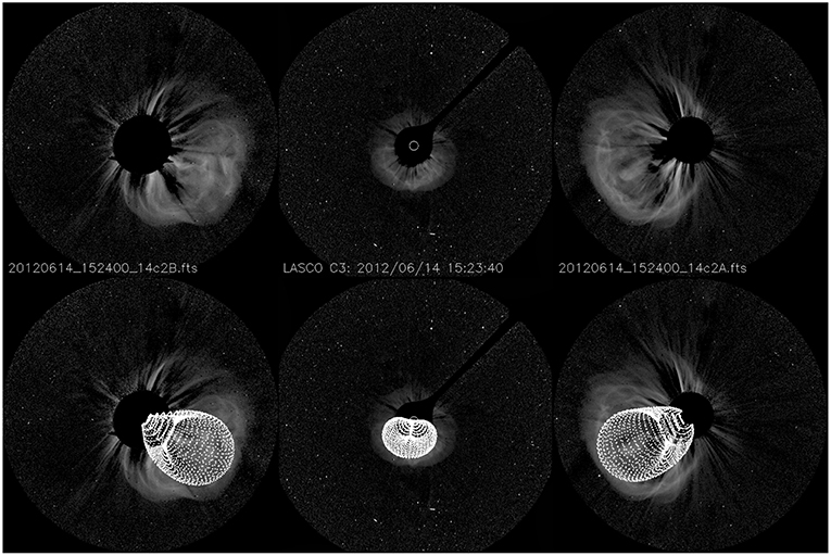
Figure 2. Example of GCS fitting of CME3 using images at 15:24 UT from STEREO/SECCHI/COR2-B (Left), SOHO/LASCO/C3 (Middle), and STEREO/SECCHI/COR2-A (Right).

TABLE 1

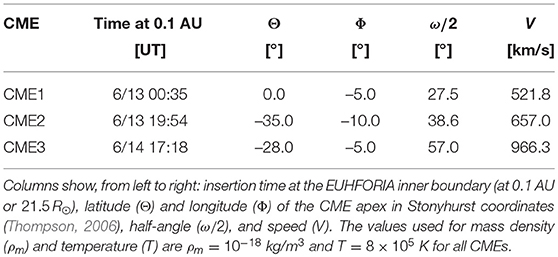
Table 1. Parameters obtained from GCS reconstructions of each CME in the outer corona and used as input to the EUHFORIA cone model described in section 3.2.

3.2. Heliospheric Observations and Modeling

We now consider the arrival of the CMEs at Venus and Earth using 3D heliospheric modeling and heliospheric imaging. In order to estimate the global propagation of the three CMEs in the heliospheric context, we perform a 3D simulation using the EUropean Heliospheric FOrecasting Information Asset (EUHFORIA; Pomoell and Poedts, 2018) model. EUHFORIA consists of a semi-empirical Wang–Sheeley–Arge (WSA; Arge et al., 2004) coronal model and a 3D time-dependent magnetohydrodynamic (MHD) heliospheric model. It allows propagation of CMEs through a steady background solar wind in the inner heliosphere from 0.1 AU onwards. We here use EUHFORIA with a cone CME model (e.g., Scolini et al., 2018) that treats CMEs as dense spheres with no internal magnetic field structure, using the input parameters presented in Table 1. The EUHFORIA simulation run for the three CMEs is shown in Supplementary Video 1. A snapshot from the simulation around the time of arrival at Earth of CME3 is shown in Figure 3. All three CMEs are seen to propagate close to the Sun–Earth line, with some differences in their latitudes. The apex of the relatively small CME1 propagates close to the ecliptic, while the propagation direction of CME2 is significantly toward the south (as expected from the latitude of −35.0° reported in Table 1). CME3 is clearly the widest and most prominent eruption in the simulation, with its apex propagating southward. However, this CME is wide enough to result in a significant component propagating along the ecliptic. The EUHFORIA simulation indicates that the three CMEs arrived at Venus in close proximity but still as mostly separated structures, while CME3 has reached the front of CME2 by the time the structures impact Earth. Finally, the merged CME2 and CME3 are seen to overtake CME1 after Earth's orbit. The arrival times of the three CMEs at Venus and Earth estimated by the EUHFORIA simulation are reported in Table 2.

FIGURE 3

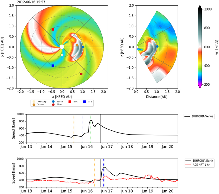
Figure 3. Snapshot of the solar wind speed simulated with EUHFORIA, showing the arrival at Earth of CME3 around June 16, 2012 at 16:00 UT. The heliographic equatorial plane (Left) and the meridional plane containing Earth (Right) are shown, together with the time series at Venus and Earth (Bottom). The arrival times of the CME-driven shocks taken from in-situ data for both locations (analyzed in section 3.3) are indicated in the time series with vertical dashed lines (CME1, orange; CME2, blue; CME3, green).

TABLE 2

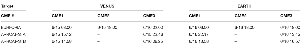
Table 2. Arrival times of the three CMEs at Venus and Earth based on EUHFORIA results and HELCATS/ARRCAT STEREO/SECCHI/HI-A and -B reconstructions.

We also follow the CMEs in heliospheric imagery. Supplementary Video 2 includes a movie of HI1-A and -B data that shows the CMEs' propagation. The HI1 observations show, in agreement with coronagraph observations and heliospheric modeling results, that CME1 was fairly narrow and propagating along the ecliptic, that CME2 propagated mostly toward the south but with a non-zero component along the ecliptic, and that CME3 was the largest of the three, expanding in latitude well beyond the HI1 field of view. HI2 observations (not shown) suggest that CME3 subsumed CME2 between the orbits of Venus and Earth.

The HELCATS (http://www.helcats-fp7.eu) project has cataloged a number of CMEs from 2007 through 2015 using the wide-angle HIs onboard STEREO. The ARRCAT catalog (Möstl et al., 2017) produced by HELCATS gives arrival times of CMEs at various locations in the solar system that are estimated with a self-similar expansion fitting of HI data with a fixed 30° CME angular half-width (SSEF30; Davies et al., 2012). According to the ARRCAT catalog (see also the discussion in Kubicka et al., 2016), CME1 made a glancing encounter with Venus and Earth, CME2 did not encounter either of these locations, and CME3 impacted Earth almost centrally. The arrival times of the three CMEs estimated in the ARRCAT catalog are listed in Table 2.

Our simulation results are thus consistent with the information reported in the HELCATS/ARRCAT catalog for the impact of CME1 and CME3 (albeit with significant differences in arrival time) while for CME2 an in-situ impact is forecasted by EUHFORIA only. We note that, in the case of CME2, the apex was propagating at a latitude of −35° (from the GCS reconstruction reported in Table 1); thus, the fixed CME half-width of 30° assumed in SSEF30 reconstructions may explain why an arrival ‘hit' is not predicted. Now considering CME1 and CME3, the discrepancies in arrival times between our EUHFORIA simulation and the ARRCAT results may arise from both the fixed half-angular width and from the circular CME front assumed in the SSEF30 model. In the EUHFORIA model, CMEs are also launched with an initial spherical cross-section, but their fronts flatten with heliocentric distance as a result of solar wind drag (e.g., Vršnak et al., 2013). Furthermore, we note that Srivastava et al. (2018) analyzed time–elongation maps based on HI data and reconstructed the fronts of CME2 and CME3 by applying the two-spacecraft version of the SSE model, i.e., the stereoscopic SSE (SSSE; Davies et al., 2013) fitting, concluding that the two CMEs would have interacted significantly before the orbit of Venus already, at a heliocentric distance of ~ 100R_⊙ (i.e., ~ 0.47 AU). We propose a later interaction of the two CMEs (at ~ 0.72 AU), as supported by the EUHFORIA simulation, heliospheric imagery, and consideration of the eruption times of CME2 and CME3 and their relative speeds. We attribute these discrepancies to the circular CME front assumed in the SSSE model and to the fact that Srivastava et al. (2018) used a CME half-width of 90° for both CME2 and CME3, while we estimated values of 38.6° and 57.0°, respectively (see Table 1). Given that CME3 was traveling faster than CME2, both of these factors would yield an earlier CME arrival (and, therefore, interaction) than was found in our EUHFORIA simulation. We further note that our EUHFORIA cone model results are consistent with the EUHFORIA simulation performed by Scolini et al. (2019) using a cone model for CME2 and a spheromak (Verbeke et al., 2019) model for CME3.

3.3. Interplanetary Observations

We now describe the in-situ observations from VEX at Venus and the L1 spacecraft (ACE and Wind) in the near-Earth solar wind. Table 3 lists the observation times of various significant features that we discuss in detail below, including some key shock and ICME ejecta parameters.

TABLE 3

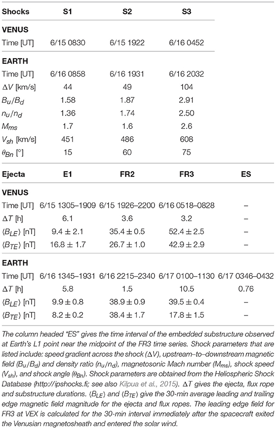
Table 3. Observation times of interplanetary shocks (S), ejecta (E) and flux ropes (FR) around Venus (in VEX data) and Earth (in Wind data).

3.3.1. Observations at Venus

Figure 4 shows magnetic field measurements, plasma parameters, and proton and electron counts (where available) measured by VEX. The magnetic field components are given in Venus Solar Orbital (VSO) coordinates.

FIGURE 4

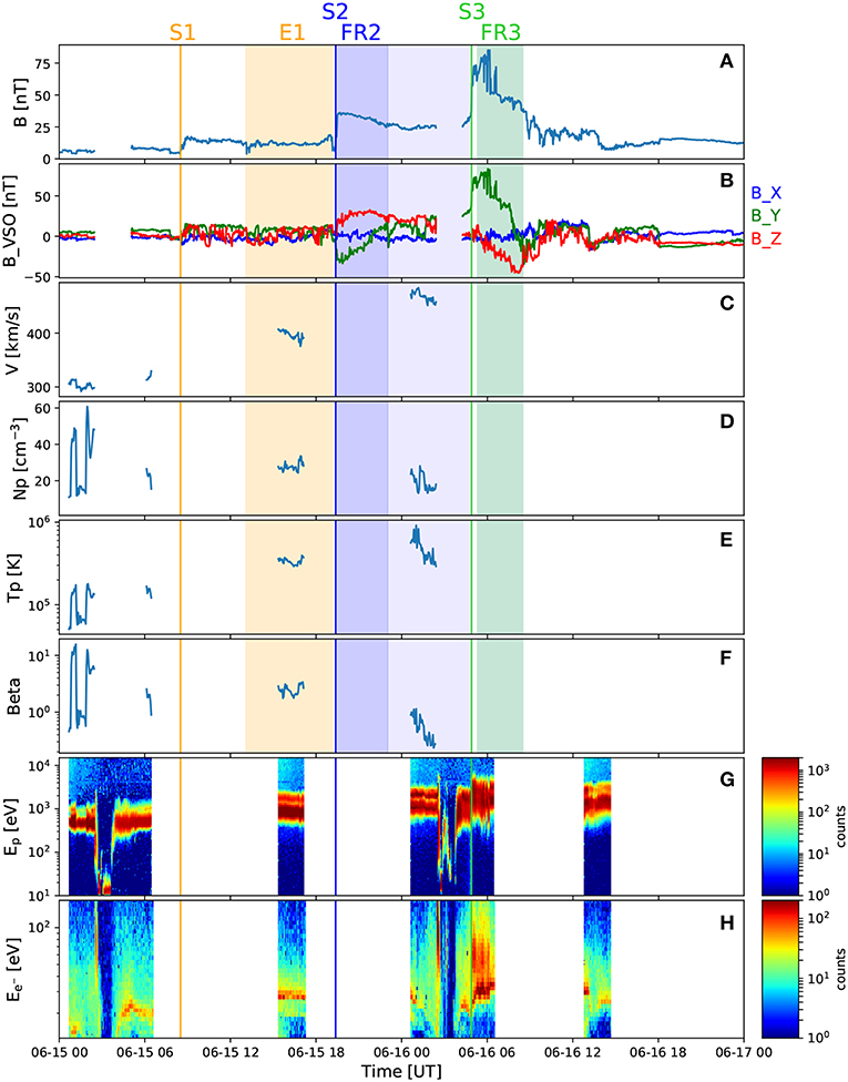
Figure 4. In-situ measurements taken by VEX around Venus. The panels show, from top to bottom: (A) magnetic field magnitude, (B) magnetic field components in VSO coordinates (blue: B_x, green: B_y, red: B_z), solar wind (C) speed, (D) density, (E) temperature, and (F) plasma beta, and counts for (G) protons and (H) electrons. The CME-driven shocks (S1, S2, and S3) are marked by vertical lines, while the ejecta and flux ropes (E1, FR2, and FR3) are highlighted with shaded regions. Intervals in the Venusian magnetosphere have been cut out from the magnetic field and plasma data. ASPERA-4, providing electron and proton counts (and from which plasma data are derived), was operational at periapsis and apoapsis only.

We interpret the increase in the magnetic field magnitude at 08:30 UT on June 15, 2012 as the shock driven by CME1 (hereafter S1). The observation time of S1 matches exactly with the arrival time of CME1 at Venus as predicted by EUHFORIA and is 6–7 h before the estimated CME1 arrival times reported in the ARRCAT catalog (see Table 2). The subsequent period with fluctuating magnetic fields represents the sheath region behind S1. On June 15, 2012 at 19:29 UT VEX entered into a flux rope (hereafter FR2) as indicated by smooth and enhanced magnetic field and the start of a steady rotation. A zoom-in around this transition region (see Supplementary Figure 1) reveals first a small field decrease on June 15 at 19:09 UT followed by a field increase at 19:22 UT. The field decrease could possibly mark the end of the ejecta related to the weak CME1 (hereafter E1, which cannot be identified robustly due to the lack of consistent plasma data at VEX), while the increase likely represents a developing shock wave (hereafter S2) driven by CME2. We also note that the magnetic field between 19:09 and 19:22 UT resembles that of the ambient solar wind, with a Parker spiral-like (Parker, 1958) configuration.

The FR2 leading edge time coincides almost exactly with the EUHFORIA prediction of the CME2 arrival at Venus (see Table 2) and this interpretation is also in agreement with observations at Earth's L1 point (see section 3.3.2). The two top panels of Figure 4 show that FR2 was characterized by an enhanced and smooth magnetic field and that the field components rotated in a coherent way. The Y-component of the magnetic field (B_Y) in FR2 at VEX rotated from negative to positive, while the Z-component of the field (B_Z) stayed positive (i.e., northward). CME2 likely continued several hours past the FR2 trailing boundary at VEX, i.e., coherent rotation of the magnetic field direction had ceased, but the field magnitude remained enhanced. As discussed by Richardson and Cane (2010) and Kilpua et al. (2013), cases where ICME signatures continue beyond the flux rope boundaries are not uncommon and could arise, e.g., from interaction with the ambient solar wind and/or erosion of the magnetic flux (e.g., Dasso et al., 2007), or represent a CME wake. VEX entered the Venusian induced magnetosphere on June 16 at 02:24 UT. The approximately 2 h interval when VEX was in the magnetosphere, until June 16 UT at 04:16 UT, has been cut out from Figure 4. The average magnetic field magnitude at the FR2 leading edge (over the first 30 min) at VEX was 35.4 nT and during the last 30 min of FR2 the field has decreased to 26.7 nT.

Approximately 1 h after VEX had traveled from the magnetosphere to the magnetosheath, the magnetic field magnitude increased abruptly on June 16 at 04:52 UT. Since outbound bow shock (BS) transitions exhibit decreases of the field magnitude rather than increases, we interpret this field jump as the interplanetary shock driven by CME3 (hereafter S3), similarly to the interpretation given by Kubicka et al. (2016). The detection time of S3 at VEX is also only 2 h later than the arrival time of CME3 predicted by EUHFORIA. The high magnetic fields after S3 represent the sheath driven by CME3 and the following flux rope (hereafter FR3) being compressed in the Venusian magnetosheath. The sharp field variations at the leading edge of FR3 are BS crossings. Supplementary Figure 2 shows a zoom-in of the VEX magnetic field data around this time. The first outbound BS crossing occurred on June 16 at 05:46 UT and the last outbound crossing at 06:37 UT. The BS crossings were partly beyond the nominal Venusian BS location (see Figure 1). We note that Zhang et al. (2008) showed that during a strong CME that impacted Venus on September 10–11, 2006 VEX observed clear BS crossings all along its trajectory even out to 12 Venusian radii. After the last outbound BS crossing, the magnetic field within FR3 is 52 nT and the field decreases to 42.9 nT by the trailing edge of FR3. We define the end boundary of FR3 where the smooth rotation ended and the magnetic field magnitude decreased. At the leading edge of FR3, B_Y was strongly positive and then rotated toward zero by the trailing edge. B_Z started from small positive values and rotated to large negative values.

3.3.2. Observations Near Earth and Comparison With Venus

Figure 5 shows observations at Earth's Lagrange L1 point; Figures 5A–C show interplanetary magnetic field (IMF) observations; the IMF magnitude, IMF components in the GSE coordinate system, and the root-mean-square of the magnetic field vector. Figures 5D–G give the solar wind plasma speed, density, temperature, and plasma beta. Figure 5F also displays the expected solar wind temperature calculated using three different approaches. The red curve is the expected temperature according to Cane and Richardson (1995) based on the solar wind–temperature relationship derived by Lopez and Freeman (1986), and which has different dependencies for slow and fast wind (break-point at 500 km/s). The light and dark orange curves are from Elliott et al. (2005) who derived a formula separately for solar wind compressions and rarefactions (based on the slopes in the 2 day averaged solar wind speed), respectively, by using a 5 year dataset from ACE and removing all ICME intervals. The solar wind oxygen charge ratio O⁺⁷/O⁺⁶ and average iron charge ratio 〈Q_Fe〉 (2 h cadence) are shown in Figures 5H,I, while the bottom Figure 5J shows the suprathermal electron 255 eV pitch angle spectrogram. Counterstreaming suprathermal electrons at 0° and 180° pitch angles are generally interpreted as a signature of closed magnetic field configurations where the field lines are connected to the Sun at both ends, while a unidirectional strahl indicates field lines that are open to the heliosphere (e.g., Zwickl et al., 1983; Gosling et al., 1987; Shodhan et al., 2000).

FIGURE 5

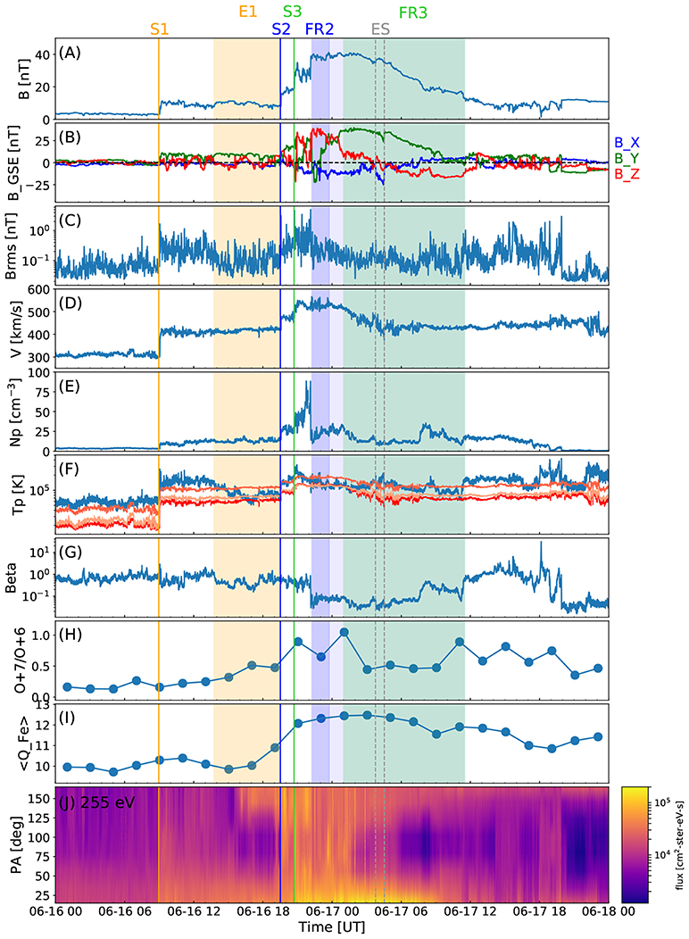
Figure 5. In-situ measurements taken at Earth's L1 point. The panels show, from top to bottom: (A) magnetic field magnitude, (B) magnetic field components in GSE coordinates (blue: B_x, green: B_y, red: B_z), (C) root-mean-square magnetic field vector (B_rms), and solar wind (D) speed, (E) density, (F) temperature (the blue curve is the measured temperature and the red/orange curves indicate the expected temperatures. The red line is from Cane and Richardson (1995), light and dark orange from Elliott et al. (2005) for the rarefactions and compression, respectively; see section 3.3.2 for details), (G) plasma beta, (H) oxygen charge state ratio, (I) average iron charge state, and (J) pitch angle spectrogram of suprathermal 255 eV electrons. The 1 m IMF and 3 s solar wind plasma data are from the Wind spacecraft, while the 2 h charge state data are from the ACE spacecraft. Red solid lines show the interplanetary shocks (S1, S2, and S3). Flux rope intervals are indicated by the dark blue and green shaded regions for FR2 and FR3, respectively; though still associated with the CME2 ejecta, the pale blue shaded region is identified as not being part of FR2. The embedded substructure (ES) is bounded by a pair of dashed gray lines.

The comparison of Figures 4, 5 shows some obvious similarities as well as several differences between the structures detected at Venus and at Earth. Similarly to Venus, the sequence of events at Earth began with shock S1 that was detected on June 16 at 08:58 UT by Wind. This shock time is only 3 h later than the predicted CME1 arrival time at Earth by EUHFORIA, and 5 and 12 h earlier than reported in the HELCATS/ARRCAT catalog for STEREO-A and -B, respectively (see Table 2). The plasma data reveal lower temperatures than during the first 4–5 h after the shock and counterstreaming suprathermal electrons starting around June 16, 13:45 UT and continuing until a shock was observed at 19:31 UT on June 16. This interval, shaded in orange in Figure 5, likely represents the ejecta related to the weak CME1, i.e., E1. Contrarily to Venus, where CME1 was followed by two separate flux ropes and from which only the latter one drove a well-developed shock, at Earth two close-by shocks were observed followed by one apparently coherent flux rope structure. The first of these shocks (S2) was observed at 19:31 UT and the other shock (S3) only about an hour later at 20:32 UT. Table 3 shows that of the three shocks detected at L1, S3 was clearly the strongest, being associated with the largest speed jump and shock speed, and the largest upstream–to–downstream magnetic field magnitude and density ratios, and magnetosonic Mach number. It was also the most perpendicular shock, with the shock angle θ_Bn being 75°.

The flux rope following S3 featured several classic ICME flux rope signatures (e.g., Zwickl et al., 1983; Richardson and Cane, 2004; Zurbuchen and Richardson, 2006; Kilpua et al., 2017a): enhanced magnetic field magnitude, a coherent rotation of the magnetic field components, some decrease in the field variability, low plasma beta, and enhanced oxygen charge ratio O⁺⁷/O⁺⁶ and average iron charge ratio 〈Q_Fe〉. The measured temperatures were generally high throughout the flux rope structure, being momentarily below only the Elliott et al. (2005) expected temperature curve for compressions. Figure 5J shows intervals of counterstreaming suprathermal electrons toward the end of the event.

Our interpretation is that shock S2 at 19:31 UT was driven by CME2 and the closely following shock S3 was driven by CME3, and thus that S3 had propagated through CME2 during the transit from Venus to Earth. In our EUHFORIA simulation run, the arrival of CME2 and CME3 cannot be separated, but their joint arrival time on June 16 at 18 UT corresponds well with the observed shock times. The arrival time of S3 at Wind is also only about 4 h later than CME3 arrival time reported in the ARRCAT catalog for STEREO-B, while the difference is a few hours larger for STEREO-A.

As discussed above, observations following S3 near Earth feature a coherent flux rope and this interval has indeed been interpreted as a single flux rope in previous studies (e.g., Kubicka et al., 2016; Palmerio et al., 2017; Srivastava et al., 2018; Good et al., 2019) and in online ICME catalogs. We suggest, in contrast, that the flux rope structure at L1 consists of two coalesced flux ropes related to CME2 and CME3, i.e., that these CMEs, which at VEX were just about to start interacting, had coalesced into one coherent structure by the time they had reached Earth's orbit. This interpretation is also supported by our EUHFORIA simulation run showing that the fast and prominent CME3 starts overtaking the slower CME2 approximately around the orbit of Venus and then engulfs it (see section 3.2 and Supplementary Video 1). We also note that there were no other possible significant CMEs that could have arrived to Venus or Earth during this period.

We have marked the possible intervals featuring the flux ropes related to CME2 and CME3 at Earth's L1 point in Figure 5 with blue- and green-shaded regions and labeled them FR2 and FR3, respectively. The lighter blue region after FR2 likely represents the part of CME2 that did not contain flux rope signatures, as discussed previously (see section 3.3.1 and Figure 4). FR2 was thus compressed from 3.6 h at VEX to 1.5 h at Earth's L1 point and its magnetic field magnitude was higher by a few nanoteslas (see Table 3). FR3, in turn, has expanded from 3.2 h at VEX to 10.5 h at Earth's L1 point. Note that the FR3 duration around Venus is underestimated because its front part was compressed in the Venusian magnetosheath. From Venus to Earth, the leading edge field of FR3 had slightly decreased, but the trailing edge field was considerably lower, falling from 42.9 nT to 17.8 nT.

The interface between FR2 and FR3 has been selected to coincide with the end of the high density region and negative–to–positive signature in B_Y. The front part of FR2 also features enhanced temperatures and solar wind speed. However, we note that this interface time is not unambiguous. In order to test our interface identifications, we have applied the mapping technique described by Good et al. (2018) in Figure 6 for the FR2 and FR3 intervals separately. In outline, the technique maps the magnetic field time series of a flux rope at an inner spacecraft (VEX in the present case) to the radial distance of an outer, aligned spacecraft (Wind) located further away from the Sun. The leading and trailing edges of the mapped profiles are constrained to overlap with the corresponding edges observed at the outer spacecraft, and the field vectors through the flux rope are mapped with a mean linear speed profile derived from the mean propagation speeds of the rope edges. The field vectors of the outer and mapped inner spacecraft profiles are normalized to the field magnitude to emphasize similarities (or dissimilarities) in the underlying flux rope structure. Figure 6 shows significant similarities in the flux rope field components and direction angles for FR3, with a more approximate similarity seen in FR2. These mappings give some support for the interface locations identified. We also note that with this interface selection, FR3 features some higher speed and fields at its leading edge. In the end part of FR3 the speed profile is almost steady, signifying the FR3 has relaxed considerably and adjusted to the speed of the trailing solar wind.

FIGURE 6

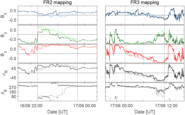
Figure 6. Mapping of the magnetic field data between VEX (pale-colored lines) and Wind (dark-colored lines) for FR2 (Left) and FR3 (Right). Details of the technique are given by Good et al. (2018). The panels show the normalized field components in the SCEQ coordinate system and the field latitude and longitude angles. Vertical dashed lines denote the flux rope boundaries.

The end boundary of FR3 is selected at the point where the plasma beta increased and the most coherent field rotation ended. This boundary coincided with the end of the flux rope included in the Wind ICME list (https://wind.nasa.gov/ICMEindex.php, Nieves-Chinchilla et al., 2018). Again, some ICME-related signatures continued for a few hours after the marked end time; for example, the field magnitude profile was relatively smooth, and O⁺⁷/O⁺⁶ and 〈Q_Fe〉 remained elevated.

We identify a small and distinct substructure within FR3 on June 17 between 03:46 UT and 04:32 UT. This substructure is marked as “ES” in Figure 5 and its boundaries are indicated by a pair of dashed vertical lines. Figure 7 shows a zoomed-in view of the substructure, highlighting that it was bounded by a pair of sharp field changes that suggest the presence of current sheets. The magnetic field components are shown here in the minimum variance analysis (MVA, see section 4.1) coordinate system, where the maximum variance component is marked in pink, the intermediate variance component in lime and the minimum variance component in light blue. The MVA has been performed over the substructure interval. Compared to its surroundings, the substructure features a slight enhancement in the magnetic field magnitude and temperature, but lower density and plasma beta. The solar wind speed shows a declining trend throughout the substructure. The intermediate and minimum variance components are relatively steady over the substructure, while the maximum variance component rotates from slightly negative to positive values. Hence, this substructure does not show signatures of a magnetic reconnection exhaust (e.g., Gosling et al., 2005), i.e., a decreased magnetic field magnitude coinciding with enhanced densities and temperatures, and the maximum variance component showing a large change in the field orientation. We also note that the substructure here occurred concurrently with the B_Z component changing sign within FR3. It could thus be similar to substructures studied, e.g., by Dasso et al. (2007) and Steed et al. (2011). They occurred near the centers of CME flux ropes and were interpreted to arise from interaction with the ambient solar wind causing warping of the flux surfaces as, at this point, the spacecraft path is almost tangential to the magnetic flux surfaces of the flux rope.

FIGURE 7

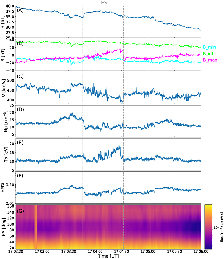
Figure 7. The embedded substructure (ES) in FR3 observed at Earth's L1 point. The ES is bounded by the vertical dashed lines. The panels show, from top to bottom: (A) magnetic field magnitude, (B) magnetic field components in MVA coordinates (light blue: B_min, lime: B_int, pink: B_max), solar wind (C) speed, (D) density, (E) temperature, (F) plasma beta, and (G) the pitch angle spectrogram of suprathermal 255 eV electrons. The 3 s IMF and solar wind plasma data are from the Wind spacecraft.

4. Analysis of the in-situ Flux Ropes

4.1. Reconstruction Techniques

Minimum variance analysis (MVA), Lundquist fitting (LQF), and Gold-Hoyle fitting (GHF) have been used to determine the orientation of the flux ropes at Venus and Earth. These relatively simple in-situ reconstruction techniques allow global parameters of a flux rope to be estimated from local observations made along the spacecraft trajectory.

MVA involves determining the eigenvalues and eigenvectors of the covariance matrix of the magnetic field vector components (Sonnerup and Cahill, 1967). The eigenvector associated with the eigenvalue of intermediate variance ideally corresponds to the flux rope axis direction (Goldstein, 1983). MVA accuracy is greater when the spacecraft intersects the flux rope near its central axis (i.e., a low impact parameter encounter; Gulisano et al., 2007) and when the variance directions are well defined. This latter condition may be assessed through the ratio of the maximum and intermediate eigenvalues, λ₁/λ₂, and the minimum and intermediate eigenvalues, λ₃/λ₂. Ratios of λ₁/λ₂ > 1.37 and λ₃/λ₂ < 0.72 are typically applied as thresholds for well-defined variance directions (Siscoe and Suey, 1972). We note that a recent study by Démoulin et al. (2018) questions the validity of eigenvalue ratios as a measure of MVA accuracy when determining flux rope axis directions.

LQF uses Bessel functions to model the flux rope field structure (Burlaga, 1988; Lepping et al., 1990). The simplest form of LQF models the flux rope as an axisymmetric cylinder with a circular cross section, in which the component of the magnetic field along the cylinder axis, B_z, and the poloidal component, B_ϕ, are given by:

$\begin{array}{ll}{B}_z^L=B_0{J}_0(\alpha r)& (1)\end{array}$

$\begin{array}{ll}{B}_{\varphi }^L=H{B}_0{J}_1(\alpha r),& (2)\end{array}$

respectively, where B₀ is the field strength at the rope axis, J₀ and J₁ are the zeroth- and first-order Bessel functions, respectively, H is the rope handedness (+1 or –1 for a right- or left-handed rope, respectively), r is the radial distance from the axis, and α is a constant. The field component in the radial direction is zero. Following a common convention, we locate the flux rope boundaries at the first zero of J₀; thus the field at the boundaries has no axial component and is purely poloidal.

In GHF (Gold and Hoyle, 1960), the flux rope field components are given by:

$\begin{array}{ll}{B}_z^G=\frac{B_0}{1+{\tau }^2{r}^2}& (3)\end{array}$

$\begin{array}{ll}{B}_{\varphi }^G=\frac{\tau r{B}_0}{1+{\tau }^2{r}^2},& (4)\end{array}$

where the twist, τ, gives the number of complete field–line turns per AU. The Gold–Hoyle solutions were first used to fit an interplanetary flux rope by Farrugia et al. (1999). In contrast to the Lundquist rope, in which twist is at a minimum at the axis and infinite at the boundaries, the τ profile across the Gold–Hoyle rope is uniform. As in LQF, the simplest form of GHF assumes a cylindrically symmetric rope geometry with a circular cross section. We locate the rope boundaries at a distance of 1/τ from the rope axis, following the convention of Hood and Priest (e.g., Hood and Priest, 1979).

LQF and GHF are performed with a three-stage, reduced χ² minimization of the model field components to the observed, normalized magnetic field time series. This minimization technique has previously been applied by Good et al. (2019). The flux rope orientation previously obtained from MVA is used as the rope's initial estimate as input for the first minimization of χ², which yields fitting F1. The minimization is then repeated with F1 as the initial orientation to give fitting F2, and repeated again with F2 as the initial orientation to give fitting F3. F2 is taken as the final reported fit, and the angle between the F2 and F3 axis orientations, δ, is used as a measure of fit sensitivity to the initialization parameters. Ideally, δ will be zero; non-zero δ values indicate that convergent fits with similar χ² values can be obtained for a range of fit parameters, i.e., that there is some elongation to the χ² minimum. The value of B₀ is determined separately with the procedure described by Lepping et al. (2003) using the F2 fit parameters.

LQF and GHF provide a range of global flux rope parameters, including the axis direction latitude and longitude angles, θ₀ and ϕ₀, respectively, B₀, H, τ (in GHF), and spacecraft impact parameter, p. The value of p ranges from 0 for spacecraft trajectories intersecting the rope axis to 1 for a skimming intersection at the rope's outer surface. With an estimate of the flux rope diameter, R, and length, L, it is also possible to estimate the magnetic flux content of the ropes. In the Lundquist rope, the axial and poloidal fluxes are approximately given by:

$\begin{array}{ll}{F}_z^L=1.4B_0{R}^2& (5)\end{array}$

$\begin{array}{ll}{F}_{\varphi }^L=\frac{B_0}{2.4}RL,& (6)\end{array}$

and in the Gold-Hoyle rope, the corresponding fluxes are given by:

$\begin{array}{ll}{F}_z^G=\frac{B_0\pi ln(1+{\tau }^2{R}^2)}{{\tau }^2}& (7)\end{array}$

$\begin{array}{ll}{F}_{\varphi }^G=\frac{B_{0}Lln(1+{\tau }^2{R}^2)}{2\tau }.& (8)\end{array}$

Derivations of Equations (5–8) are found in Dasso et al. (2006), and references therein. These expressions are valid for cylindrical ropes with circular cross-sections.

4.2. Reconstruction Results

Fitting results are given in Table 4. Fits have been performed that treat FR2 and FR3 as a single flux rope (listed under “FR2+FR3” in Table 4) and as separate flux ropes at both Venus and Earth. Figure 8 displays the LQF and GHF reconstructions (red and blue lines, respectively) of the flux ropes treated separately. The FR2 and FR3 intervals in Figure 8 are shaded as in previous figures. Fittings have been made to magnetic field data in the Spacecraft–Equatorial (SCEQ) coordinate system; note that Figures 4, 5 display data in VSO and GSE coordinates, respectively. At both spacecraft, the flux ropes could be fitted relatively well with both methods. Table 4 gives two quality-of-fit measures for the GHF and LQF, namely, the δ initiation sensitivity angle and the minimized χ² values associated with the fits (see section 4.1); for all fits listed, the δ and χ² values are relatively low and consistent with accurate fits. The MVA eigenvalue ratios met the Siscoe and Suey (1972) conditions for well-defined variance directions (see section 4.1).

TABLE 4

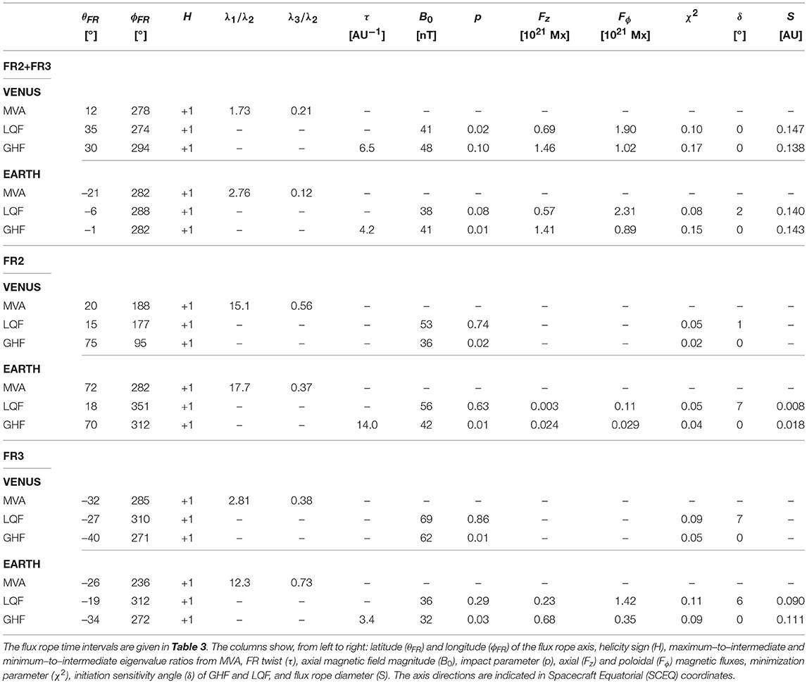
Table 4. MVA, GHF, and LQF results for FR2 and FR3 treated as a single structure and separately.

FIGURE 8

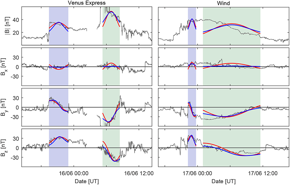
Figure 8. Gold-Hoyle fits (blue lines) and Lundquist fits (red lines) to the magnetic field data at VEX (Left) and Wind (Right) separately for FR2 (blue-shaded interval) and FR3 (green-shaded interval). Measurements made in the Venusian magnetosphere have been removed. The panels show, from top to bottom, the magnetic field magnitude and the three field components in Spacecraft Equatorial (SCEQ) coordinates. The SCEQ coordinate system is identical to the Heliocentric Earth Equatorial (HEEQ; Thompson, 2006) system at the locations of Earth and the Sun–Earth L1 point.

Fits to the combined FR2+FR3 interval at both spacecraft indicate a rope axis that was directed approximately toward the solar east direction, i.e., ${\varphi }_{FR}~270^{°}$. This was found consistently with all three reconstruction techniques. Axis inclination ϕ_FR for all reconstructions was higher at Venus than at Earth, with the difference varying from 31° for GHF to 41° for LQF. Fits to the FR2+FR3 interval at Earth performed in previous studies are consistent with our fit results: Palmerio et al. (2017) applied Grad–Shafranov reconstruction (GSR; e.g., Hu and Sonnerup, 2002; Isavnin et al., 2011) obtaining an axis orientation of ${\varphi }_{FR}=299^{°}$ and ${\theta }_{FR}=6^{°}$; Nieves-Chinchilla et al. (2018) used the circular-cylindrical flux rope analytical model (Nieves-Chinchilla et al., 2016) to obtain an axis orientation of ${\varphi }_{FR}=297^{°}$ and ${\theta }_{FR}=-3^{°}$. We also note that our fits had a positive chirality (helicity sign) at both Venus and Earth. This is consistent with the analysis of indirect solar proxies (see Section 3.1 and Palmerio et al., 2017), the hemispheric helicity rule (e.g., Seehafer, 1990; Bothmer and Schwenn, 1998; Pevtsov and Balasubramaniam, 2003), and with the presumption of helicity sign conservation (e.g., Woltjer, 1958; Berger, 2005).

Table 4 also lists estimates of the flux rope diameter, S. At Wind, these estimates are derived from the flux rope's passage time and mean proton speed, and take into account the axis orientations and spacecraft impact parameters obtained from the fits. For the FR2+FR3 interval at Wind, the mean proton speed was ~ 439 km/s, yielding S = 0.140 AU for LQF and S = 0.143 AU for GHF. At VEX, a burst of speed measurements averaging ~ 468 km/s is used to determine S values of 0.147 AU in LQF and 0.138 AU in GHF. The τ, F_z, and F_ϕ values listed in Table 4 (and discussed below) are functions of R = S/2.

We now consider the fits made to FR2 and FR3 separately, as displayed in Figure 8. Fitting results for FR2 varied considerably between the different techniques. At Venus, MVA and LQF gave a low inclination axis pointing toward the Sun, while GHF gave a highly (northward) inclined, eastward tilted axis. At Earth, in contrast, MVA and GHF both gave a highly inclined axis tilted toward the east, while LQF gave a low inclination, antisunward-directed axis. At both Venus and Earth, LQF estimated considerably higher p and B₀ values than GHF. Some indication of the origin of these differences can be seen in Figure 8, which shows quite different reconstructions for B_X between LQF and GHF; the flatter B_X of the GHF better captures the observed profile. However, the large impact parameters found in LQF are consistent with the apex of CME2 propagating toward the south, as seen in remote sensing observations (see Table 1 and Supplementary Video 2) and EUHFORIA modeling (see Figure 3 and Supplementary Video 1). Estimates of S suggest that FR2 was very small in size by the time of arrival at Earth. S has not been determined at Venus for FR2 or FR3 because suitable speed measurements were lacking. The reconstructions presented for FR2 should be considered only as approximations due to the short duration of the event, interactions, and potentially off-centers encounter (e.g., Al-Haddad et al., 2013).

Fitting orientations for FR3 are much more consistent across the different fitting techniques. They all indicate, at both Venus and Earth, an approximately eastward directed rope with a moderate inclination toward the south. It is notable that each technique indicates a slight reduction in inclination (i.e., | θ_FR | reducing) from Venus to Earth; such reductions with heliocentric distance have been observed previously (e.g., Good et al., 2019). However, p values for LQF and GHF differ significantly; as with FR2, this is partly a result of differences in reconstruction of the B_X component. The diameter S of FR3 was much greater than that of FR2 at Earth.

The magnetic flux content of the ropes have been obtained with Equations 5–8 and parameters from the fits. The axial (F_z) and poloidal (F_ϕ) flux values are listed in Table 4. In order to obtain the F_ϕ values, the flux rope length L has been estimated to equal 2πγR/180°, i.e., L spans the arc length defined by the angle 2γ, where γ is the half-angle between the CME legs obtained from the GCS reconstructions (see section 3.1). CME2 and CME3 had γ values of 15° and 27°, respectively; these give L values for FR2 and FR3 of 0.38 AU and 0.68 AU at Venus, and 0.52 and 0.94 AU at Earth, respectively. For the FR2+FR3 interval, the FR3 L values are used. First considering the FR2+FR3 interval, it can be seen that the total flux content at Venus and Earth was comparable in both LQF and GHF. Total flux from the LQF was 2.59 × 10²¹ Mx at Venus and 2.88 × 10²¹ Mx at Earth; the corresponding values from GHF were 2.48 × 10²¹ Mx and 2.30 × 10²¹ Mx, respectively. The flux is distributed more poloidally than axially in the LQF than in the GHF due to the nature of the respective model fields. Treating the flux ropes separately, both LQF and GHF estimated low flux content in FR2 at Earth, reflecting its small size, while FR3 contained a considerably larger amount of flux.

As discussed in section 3.3.2, FR2 had contracted significantly by the time it reached Earth and, in any case, it represented only a glancing encounter through the northern part of the larger flux rope related to CME2. The resulting fluxes (in particular, $F_{\varphi }=0.11\times 10^{21}$ Mx from LQF and $F_{\varphi }=0.029\times 10^{21}$ Mx for GHF) are thus small and considerably below (by one to two orders of magnitude) the values derived from solar analysis (see section 3.1, where $F_{\varphi }=0.5\times 4.60\times 10^{21}=2.30\times 10^{21}$ Mx from PEA analysis and $F_{\varphi }=0.5\times 2.21\times 10^{21}=1.11\times 10^{21}$ Mx from ribbon analysis). For FR3, the poloidal flux values estimated at Wind are equal to $F_{\varphi }=1.42\times 10^{21}$ Mx from LQF and $F_{\varphi }=0.35\times 10^{21}$ Mx from GHF. The poloidal flux from LQF is thus smaller but of the same order of magnitude as the fluxes estimated from solar observations (see section 3.1, where $F_{\varphi }=0.5\times 6.04\times 10^{21}=3.02\times 10^{21}$ Mx and $F_{\varphi }=0.5\times 3.88\times 10^{21}=1.94\times 10^{21}$ Mx for PEA and ribbon analyses, respectively), whereas the GHF estimates are an order of magnitude smaller than the solar estimates.

Estimates of magnetic flux in CME flux ropes are subject to large uncertainties. In the case of in-situ estimates, uncertainties are related to the length L of the flux rope loop, fitting parameters, distribution of magnetic flux in the flux rope, knowledge of the true cross-sectional shape, and the possible occurrence of erosive reconnection in interplanetary space (e.g., see discussion in Möstl et al., 2008). For example, if CME flux ropes flatten normal to their propagation direction as they travel through interplanetary space, in-situ flux values are expected to be underestimated by cylindrical models (Owens, 2008), and thus lower than those obtained from solar observations. Such a discrepancy between solar and in-situ estimates has been found in our analysis, and also in several previous works (e.g., Longcope et al., 2007; Qiu et al., 2007; Möstl et al., 2008; Lynch et al., 2010). We further note that estimates for the events analyzed here are complicated by interactions and off-center encounters, particularly for FR2. Recent studies have also emphasized difficulties in the present flux rope fitting techniques, e.g., for detecting writhe (e.g., Al-Haddad et al., 2019). Due to these constraints and the complexity of the events studied, we stress that the flux values are approximate and no firm conclusions should be drawn from them.

5. Summary and Discussion

In this work, we have analyzed the interplanetary counterparts of three CMEs that erupted from the Sun between June 12 and 14, 2012 using multipoint measurements from VEX at 0.7 AU, and from Wind and ACE at 1 AU. During the investigated period, Venus and Earth were separated by 5.4° in longitude and by 0.2° in latitude, i.e., they very close to radial alignment.

Our analysis of remote-sensing data from the solar disc through the inner heliosphere combined with a careful investigation of in-situ measurements supported by 3D heliospheric modeling suggests the following scenario: the first CME (CME1; launched on June 12, 2012 as two sympathetic eruptions that merged close to the Sun) encountered Venus and Earth quite centrally as it propagated along the ecliptic and close to the Sun–Earth line. The most prominent signatures of CME1 detected at Venus and at Earth were a shock and a turbulent sheath. Plasma data also revealed that a magnetic ejecta (E1), featuring lower temperatures and counterstreaming electrons, was likely encountered by Wind. A magnetic cloud structure was likely missing because interaction of the two sympathetic eruptions at the Sun produced a complex ejecta (e.g., Burlaga et al., 2002). The second and third CMEs (CME2 and CME3; launched on June 13, 2012 and June 14, 2012, respectively) arrived in succession at Venus, producing two separate flux rope (FR2 and FR3) intervals. Soon after the passage of FR2, VEX moved into Venus's induced magnetosphere for 2 h. The shock driven by CME3 (S3) and the following FR3 arrived at Venus when VEX was back in the magnetosheath on the nightside; the sheath and the front part of FR3 were thus compressed in the Venusian magnetosheath. Due to solar wind preconditioning provoked by the preceding CMEs, CME3 likely propagated out to Venus's orbit experiencing relatively little solar wind drag, thus maintaining its high speed and magnetic field magnitude (e.g., Liu et al., 2014). Significant interactions occurred between Venus and Earth; the shock driven by CME3 propagated through CME2 and resulted in a closely-based double shock signature before FR2 at Earth's L1 point. Both simulation and observational studies have shown that the shock of a faster CME can propagate through a slower preceding CME and that their shocks may finally merge into a single, stronger shock (e.g., Odstrcil et al., 2003; Farrugia and Berdichevsky, 2004; Wu et al., 2004; Xiong et al., 2007; Lugaz et al., 2013).

Observations at Earth's L1 point showed that CME3 had compressed CME2 to create a structure resembling one coherent flux rope. Compared to measurements at Venus, the flux ropes FR2 and FR3 had mostly maintained their integrity. This is in agreement with the trailing part of FR2 and its wake having had fields directed in a roughly similar direction as those at the leading edge of FR3. Thus, no significant magnetic reconnection is expected to have occurred between these two CMEs.

On average, the magnetic field magnitudes in ICMEs decrease with increasing distance from the Sun as a result of expansion (e.g., Richardson et al., 2006). For example, Leitner et al. (2007) obtained the radial dependence $r_H^{-1.64\pm 0.4}$ (where r_H is the radial distance from the Sun) from their analysis of 130 magnetic clouds observed during the Helios era between 0.3 and 1 AU. Using this approximate dependence, the leading edge field of 35.6 nT for FR2 at Venus would have dropped to about 20 nT by the time it had reached Earth's orbit. In the case of FR2, the magnetic fields were now instead slightly higher at Earth than at Venus. The high magnetic fields observed at Earth (~40 nT) were thus partly related to the compression of CME2, i.e., not only to the fast and prominent CME3, which, according to remote-sensing observations, appeared as the most obviously Earth-directed CME. In their simulation study, Schmidt and Cargill (2004) investigated cases where a faster and high-B CME and a slower and low-B CME interact at their flanks, i.e., in a similar fashion to our case. The two cases studied, one where the interacting CMEs have the same chirality and the other where the CMEs have opposite chirality, are presented in their Figures 4, 5, respectively. Both scenarios result in contraction of the leading CME at the point of interaction and enhancement of the field. Similar cases have also been analyzed e.g. by Lugaz et al. (2013), where contraction of a leading CME and relaxation of a trailing CME were observed. However, the details of CME–CME interaction depend strongly on the specific properties and directions of the interacting CMEs.

As discussed in section 3.3, the combined structure consisting of FR2 and FR3 at Earth has been treated as a single flux rope (linked to CME3) in previous studies. However, when considering observations at Venus, this interpretation is clearly problematic. There are no other CMEs in a suitable time window that could have caused such a strong interplanetary shock to propagate through CME3. In this single-rope scenario, the flux rope would have also had to rotate by about 30–40° between Venus and Earth (see our reconstruction results from Table 4), due either to radial evolution or to the flux rope being highly warped over small longitudinal distances. As noted in the Introduction, significant changes in the tilts of flux rope axes have been reported in multi-spacecraft studies, but were mostly connected to cases where the observing spacecraft have been separated by at least a few tens of degrees in longitude.

We emphasize the ambiguity in determining the interface between FR2 and FR3 at Earth due to CME–CME interaction and the interplanetary counterpart of CME2 featuring a wake after FR2 (as discussed in section 3.3.1, the ICME ejecta-like magnetic field signatures continued beyond the FR2 trailing boundary). We note, however, that our selected FR2 and FR3 intervals show clear similarities between Venus and Earth when compared through a direct mapping technique, and this interpretation also better matches with the observed speed profile at Wind. The substructure we identified within FR3 did not show signatures of a reconnection exhaust. We conclude that it either represented a warping of flux surfaces near the center of the flux rope, as suggested by Dasso et al. (2007), or to have been formed spontaneously due to the flux rope kinematic propagation (Owens, 2009). We also note that the solar wind density was high at Earth in FR2 and temperatures were relatively enhanced throughout the whole FR2 and FR3 interval, particularly during the passage of FR2 and the front part of FR3. The plasma beta, however, was depressed during the passage of both flux ropes, consistent with the findings of Farrugia and Berdichevsky (2004) who analyzed interacting CMEs using in-situ observations by Helios and ISEE.

As discussed above, the magnetic field characteristics of FR3 were quite similar at the two observation points. While the flux rope axis orientation matched relatively well (within ~ 10° for LQF and GHF) for FR3 between Venus and Earth, the FR2 reconstruction results were less consistent, possibly due to the significant compression and spacecraft crossings made far from the flux rope axis. Kubicka et al. (2016) concluded that observations at VEX for this CME–CME interaction event yielded a good proxy of the corresponding geomagnetic storm strength at Earth. This likely results from the flux ropes roughly maintaining their integrity despite significant interaction. Were reconnection and drastic merging of the CMEs to have occurred between Venus and Earth, it is likely that the prediction of a storm would have been less accurate. However, the results indicate that, in some interacting CME cases at least, a probe at the distance of Venus could be used successfully for space weather forecasting (see also Lindsay et al., 1999). One possibility to obtain consistent solar wind monitoring closer to the Sun is the placement of identical probes in orbit about the Sun, e.g., at the orbit of Venus (Ritter et al., 2015; Törmä, 2016) or in orbit around Earth in a diamond-like configuration (Cyr et al., 2000). The aim is to have such a large grid of monitors that at least one of them would always encounter any Earth-impacting CME. The accuracy of forecasting using these approaches is, however, significantly influenced by any considerable change over small spacecraft separations (as suggested e.g., by Kilpua et al., 2011; Lugaz et al., 2018; Good et al., 2019) and significant evolution or interaction of CMEs over relatively small radial distances.

In conclusion, we have highlighted in this paper the complexity of interpreting interplanetary observations made during interacting CME events. During the investigated period, remote-sensing observations showed only one clearly Earth-directed CME that was fast and prominent, with a single coherent flux rope being detected in situ at Earth. Measurements taken by VEX around Venus were crucial for revealing that this coherent flux rope structure at Earth was actually composed of two coalesced flux ropes, the first being embedded in an edge-encountered CME and compressed by the following CME. Together, they produced the strongest magnetic field magnitudes observed in the near-Earth solar wind during Solar Cycle 24. Although Earth and Venus were almost radially aligned and separated by only 0.28 AU in radial distance, the spacecraft at these locations observed interaction between the two successive CMEs at very different phases: VEX observed the interaction just prior to onset, while the spacecraft at Earth's L1 point made observations when the interaction was almost complete. A considerable interaction thus occurred over a relatively short radial distance. Our study also highlights the importance of heliospheric modeling and imaging for building a comprehensive picture of CMEs and their interactions in interplanetary space.

Author Contributions

EK: in-situ analysis and interpretation, primary responsibility for drafting the text, and combining different elements of the analysis. SG: in-situ analysis and interpretation, flux rope fitting and mapping, and text composition. EP: solar, coronagraph, and heliospheric remote-sensing observations and interpretation, Venus in-situ analysis, and text composition. EA: CME reconstructions at the Sun and EUHFORIA simulation. EL: solar observations and estimation of magnetic flux at the Sun. MA-L: earth in-situ analysis (substructure). MK, DM, and DP: analysis of solar observations. JP: EUHFORIA simulation, heliospheric evolution. JM and SP: EUHFORIA simulation. YF: Venus in-situ data analysis and interpretation. All of the authors read and critically revised the paper, approved the final version, and agreed to be accountable for all aspects of the work.

Funding

This work was supported by funding from the SolMAG project (ERC-COG 724391) funded by the European Research Council (ERC) in the framework of the Horizon 2020 Research and Innovation Programme, the BRAIN-be project CCSOM, and the Academy of Finland project SMASH 310445. EK and DP were supported with funding from the Finnish Society of Sciences and Letters and the Ruth och Nils Stenbäcks stipendium. The results presented here have been achieved under the framework of the Finnish Centre of Excellence in Research of Sustainable Space (Academy of Finland grant number 312390), which we gratefully acknowledge.

Conflict of Interest Statement

The authors declare that the research was conducted in the absence of any commercial or financial relationships that could be construed as a potential conflict of interest.

Acknowledgments

EUHFORIA is developed as a joint effort between the University of Helsinki and KU Leuven. The validation of solar wind and CME modeling with EUHFORIA throughout the inner heliosphere is being performed within the BRAIN-be project CCSOM (Constraining CMEs and Shocks by Observations and Modeling; http://www.sidc.be/ccsom/). We acknowledge the European Union FP7-SPACE-2013-1 programme for the HELCATS project (#606692). EK and DP acknowledge the Finnish Society of Sciences and Letters and the Ruth och Nils Stenbäcks stipendium. We also acknowledge use of the CDAW SOHO/LASCO event catalog (https://cdaw.gsfc.nasa.gov/CME_list/), which is generated and maintained at the CDAW Data Center by NASA and the Catholic University of America in cooperation with NRL, and the STEREO/SECCHI/COR2 CME catalog (http://solar.jhuapl.edu/Data-Products/COR-CME-Catalog.php) that is generated and maintained by John Hopkins University Applied Physics Laboratory, in collaboration with NRL and the NASA Goddard Space Flight Center. The authors thank the STEREO/SECCHI consortium for providing the data (COR and HI). The SECCHI data used here were produced by an international consortium of the Naval Research Laboratory (USA), Lockheed Martin Solar and Astrophysics Lab (USA), NASA Goddard Space Flight Center (USA), Rutherford Appleton Laboratory (UK), University of Birmingham (UK), Max-Planck-Institut for Solar System Research (Germany), Centre Spatiale de Liége (Belgium), Institut d'Optique Theorique et Appliquée (France), and Institut d'Astrophysique Spatiale (France). We acknowledge A. Szabo for the Wind/MFI data, K. Ogilvie for the Wind/SWE data, R. Lin/S. Bale for the Wind/3DP data, and G. Gloeckler for the ACE/SWICS data.

Supplementary Material

The Supplementary Material for this article can be found online at: https://www.frontiersin.org/articles/10.3389/fspas.2019.00050/full#supplementary-material

References

Al-Haddad, N., Nieves-Chinchilla, T., Savani, N. P., Möstl, C., Marubashi, K., Hidalgo, M. A., et al. (2013). Magnetic field configuration models and reconstruction methods for interplanetary coronal mass ejections. Sol. Phys. 284, 129–149. doi: 10.1007/s11207-013-0244-5

CrossRef Full Text | Google Scholar

Al-Haddad, N., Poedts, S., Roussev, I., Farrugia, C. J., Yu, W., and Lugaz, N. (2019). The magnetic morphology of magnetic clouds: multi-spacecraft investigation of twisted and writhed coronal mass ejections. Astrophys. J. 870:100. doi: 10.3847/1538-4357/aaf38d

CrossRef Full Text | Google Scholar

Arge, C. N., Luhmann, J. G., Odstrcil, D., Schrijver, C. J., and Li, Y. (2004). Stream structure and coronal sources of the solar wind during the May 12th, 1997 CME. J. Atmosp. Sol. Terrest. Phys. 66, 1295–1309. doi: 10.1016/j.jastp.2004.03.018

CrossRef Full Text | Google Scholar

Barabash, S., Sauvaud, J.-A., Gunell, H., Andersson, H., Grigoriev, A., Brinkfeldt, K., et al. (2007). The Analyser of Space Plasmas and Energetic Atoms (ASPERA-4) for the Venus Express mission. Planet. Space Sci. 55, 1772–1792. doi: 10.1016/j.pss.2007.01.014

CrossRef Full Text | Google Scholar

Berger, M. A. (2005). Magnetic helicity conservation. Highlights Astron. 13:85. doi: 10.1017/S1539299600015148

CrossRef Full Text | Google Scholar

Bothmer, V., and Schwenn, R. (1998). The structure and origin of magnetic clouds in the solar wind. Ann. Geophys. 16, 1–24. doi: 10.1007/s00585-997-0001-x

CrossRef Full Text | Google Scholar

Brueckner, G. E., Howard, R. A., Koomen, M. J., Korendyke, C. M., Michels, D. J., Moses, J. D., et al. (1995). The Large Angle Spectroscopic Coronagraph (LASCO). Sol. Phys. 162, 357–402. doi: 10.1007/BF00733434

CrossRef Full Text | Google Scholar

Burlaga, L., Sittler, E., Mariani, F., and Schwenn, R. (1981). Magnetic loop behind an interplanetary shock: Voyager, Helios, and IMP 8 observations. J. Geophys. Res. 86, 6673–6684. doi: 10.1029/JA086iA08p06673

CrossRef Full Text | Google Scholar

Burlaga, L. F. (1988). Magnetic clouds and force-free fields with constant alpha. J. Geophys. Res. 93, 7217–7224. doi: 10.1029/JA093iA07p07217

CrossRef Full Text | Google Scholar

Burlaga, L. F., Lepping, R. P., and Jones, J. A. (1990). “Global configuration of a magnetic cloud,” in Physics of Magnetic Flux Ropes, volume 58 of Geophysical Monograph eds C. T. Russell, E. R. Priest, and L. C. Lee (Washington, DC: American Geophysical Union), 373–377.

Google Scholar

Burlaga, L. F., Plunkett, S. P., and St. Cyr, O. C. (2002). Successive CMEs and complex ejecta. J. Geophys. Res. 107:1266. doi: 10.1029/2001JA000255

CrossRef Full Text | Google Scholar

Cane, H. V., and Richardson, I. G. (1995). Cosmic ray decreases and solar wind disturbances during late October 1989. J. Geophys. Res. 100, 1755–1762. doi: 10.1029/94JA03073

CrossRef Full Text | Google Scholar

Cane, H. V., and Richardson, I. G. (2003). Interplanetary coronal mass ejections in the near-Earth solar wind during 1996–2002. J. Geophys. Res. 108:1156. doi: 10.1029/2002JA009817

CrossRef Full Text | Google Scholar

Cane, H. V., Richardson, I. G., and Wibberenz, G. (1997). Helios 1 and 2 observations of particle decreases, ejecta, and magnetic clouds. J. Geophys. Res. 102, 7075–7086. doi: 10.1029/97JA00149

CrossRef Full Text | Google Scholar

Chen, J. (2017). Physics of erupting solar flux ropes: coronal mass ejections (CMEs), Recent advances in theory and observation. Phys. Plasmas 24:090501. doi: 10.1063/1.4993929

CrossRef Full Text | Google Scholar

Chi, Y., Zhang, J., Shen, C., Hess, P., Liu, L., Mishra, W., et al. (2018). Observational study of an earth-affecting problematic ICME from STEREO. Astrophys. J. 863:108. doi: 10.3847/1538-4357/aacf44

CrossRef Full Text | Google Scholar

Crooker, N. U., Gosling, J. T., and Kahler, S. W. (1998). Magnetic clouds at sector boundaries. J. Geophys. Res. 103, 301–306. doi: 10.1029/97JA02774

CrossRef Full Text | Google Scholar

Cyr, O. C. S., Mesarch, M. A., Maldonado, H. M., Folta, D. C., Harper, A. D., Davila, J. M., et al. (2000). Space weather diamond: a four spacecraft monitoring system. J. Atmos. Sol. Terrest. Phys. 62, 1251–1255. doi: 10.1016/S1364-6826(00)00069-9

CrossRef Full Text | Google Scholar

Dasso, S., Mandrini, C. H., Démoulin, P., and Luoni, M. L. (2006). A new model-independent method to compute magnetic helicity in magnetic clouds. Astron. Astrophys. 455, 349–359. doi: 10.1051/0004-6361:20064806

CrossRef Full Text | Google Scholar

Dasso, S., Nakwacki, M. S., Démoulin, P., and Mandrini, C. H. (2007). Progressive transformation of a flux rope to an ICME. Comparative analysis using the direct and fitted expansion methods. Sol. Phys. 244, 115–137. doi: 10.1007/s11207-007-9034-2

CrossRef Full Text | Google Scholar

Davies, J. A., Harrison, R. A., Perry, C. H., Möstl, C., Lugaz, N., Rollett, T., et al. (2012). A self-similar expansion model for use in solar wind transient propagation studies. Astrophys. J. 750:23. doi: 10.1088/0004-637X/750/1/23

CrossRef Full Text | Google Scholar

Davies, J. A., Perry, C. H., Trines, R. M. G. M., Harrison, R. A., Lugaz, N., Möstl, C., et al. (2013). Establishing a stereoscopic technique for determining the kinematic properties of solar wind transients based on a generalized self-similarly expanding circular geometry. Astrophys. J. 777:167. doi: 10.1088/0004-637X/777/2/167

CrossRef Full Text | Google Scholar

Démoulin, P., Dasso, S., and Janvier, M. (2018). Exploring the biases of a new method based on minimum variance for interplanetary magnetic clouds. Astron. Astrophys. 619:A139. doi: 10.1051/0004-6361/201833831

CrossRef Full Text | Google Scholar

Domingo, V., Fleck, B., and Poland, A. I. (1995). The SOHO mission: an overview. Sol. Phys. 162, 1–37. doi: 10.1007/BF00733425

CrossRef Full Text | Google Scholar

Eastwood, J. P., Biffis, E., Hapgood, M. A., Green, L., Bisi, M. M., Bentley, R. D., et al. (2017). The economic impact of space weather: where do we stand? Risk Analy. 37, 206–228. doi: 10.1111/risa.12765

PubMed Abstract | CrossRef Full Text | Google Scholar

Elliott, H. A., McComas, D. J., Schwadron, N. A., Gosling, J. T., Skoug, R. M., Gloeckler, G., et al. (2005). An improved expected temperature formula for identifying interplanetary coronal mass ejections. J. Geophys. Res. 110:A04103. doi: 10.1029/2004JA010794

CrossRef Full Text | Google Scholar

Eyles, C. J., Harrison, R. A., Davis, C. J., Waltham, N. R., Shaughnessy, B. M., Mapson-Menard, H. C. A., et al. (2009). The heliospheric imagers onboard the STEREO mission. Sol. Phys. 254, 387–445. doi: 10.1007/s11207-008-9299-0

CrossRef Full Text | Google Scholar

Farrugia, C., and Berdichevsky, D. (2004). Evolutionary signatures in complex ejecta and their driven shocks. Ann. Geophys. 22, 3679–3698. doi: 10.5194/angeo-22-3679-2004

CrossRef Full Text | Google Scholar

Farrugia, C. J., Berdichevsky, D. B., Möstl, C., Galvin, A. B., Leitner, M., Popecki, M. A., et al. (2011). Multiple, distant (40°) in situ observations of a magnetic cloud and a corotating interaction region complex. J. Atmos. Sol. Terrest. Phys. 73, 1254–1269. doi: 10.1016/j.jastp.2010.09.011

CrossRef Full Text | Google Scholar

Farrugia, C. J., Janoo, L. A., Torbert, R. B., Quinn, J. M., Ogilvie, K. W., Lepping, R. P., et al. (1999). “A uniform-twist magnetic flux rope in the solar wind,” in American Institute of Physics Conference Series, Solar Wind Nine, eds S. R. Habbal, R. Esser, J. V. Hollweg, and P. A. Isenberg (Melville, NY: American Institute of Physics), 745–748.

Google Scholar

Feng, H., Zhao, Y., Zhao, G., Liu, Q., and Wu, D. (2019). Observations on a series of merging magnetic flux ropes within an interplanetary coronal mass ejection. Geophys. Res. Lett. 46, 5–10. doi: 10.1029/2018GL080063

CrossRef Full Text | Google Scholar

Gloeckler, G., Cain, J., Ipavich, F. M., Tums, E. O., Bedini, P., Fisk, L. A., et al. (1998). Investigation of the composition of solar and interstellar matter using solar wind and pickup ion measurements with SWICS and SWIMS on the ACE spacecraft. Space Sci. Rev. 86, 497–539. doi: 10.1023/A:1005036131689

CrossRef Full Text | Google Scholar

Gold, T., and Hoyle, F. (1960). On the origin of solar flares. Month. Not. R. Astron. Soc. 120:89. doi: 10.1093/mnras/120.2.89

CrossRef Full Text | Google Scholar

Goldstein, H. (1983). “On the field configuration in magnetic clouds,” in NASA Conference Publication, JPL Solar Wind Five, Vol. 228, ed M. Neugebauer (Washington, DC: NASA, 731–733

Google Scholar

Good, S. W., Forsyth, R. J., Eastwood, J. P., and Möstl, C. (2018). Correlation of ICME magnetic fields at radially aligned spacecraft. Sol. Phys. 293:52. doi: 10.1007/s11207-018-1264-y

PubMed Abstract | CrossRef Full Text | Google Scholar

Good, S. W., Kilpua, E. K. J., LaMoury, A. T., Forsyth, R. J., Eastwood, J. P., and Möstl, C. (2019). Self-Similarity of ICME flux ropes: observations by radially aligned spacecraft in the inner heliosphere. J. Geophys. Res. 124. doi: 10.1029/2019JA026475

CrossRef Full Text | Google Scholar

Gopalswamy, N., Yashiro, S., Akiyama, S., and Xie, H. (2017). Estimation of reconnection flux using post-eruption arcades and its relevance to magnetic clouds at 1 AU. Sol. Phys. 292:65. doi: 10.1007/s11207-017-1080-9

CrossRef Full Text | Google Scholar

Gosling, J. T. (1990). Coronal mass ejections and magnetic flux ropes in interplanetary space. Am. Geophys. Union Geophy. Monogr. Ser. 58, 343–364.

Google Scholar

Gosling, J. T., Baker, D. N., Bame, S. J., Feldman, W. C., Zwickl, R. D., and Smith, E. J. (1987). Bidirectional solar wind electron heat flux events. J. Geophys. Res. 92, 8519–8535. doi: 10.1029/JA092iA08p08519

CrossRef Full Text | Google Scholar

Gosling, J. T., McComas, D. J., Phillips, J. L., and Bame, S. J. (1991). Geomagnetic activity associated with earth passage of interplanetary shock disturbances and coronal mass ejections. J. Geophys. Res. 96, 7831–7839. doi: 10.1029/91JA00316

CrossRef Full Text | Google Scholar

Gosling, J. T., Skoug, R. M., McComas, D. J., and Smith, C. W. (2005). Direct evidence for magnetic reconnection in the solar wind near 1 AU. J. Geophys. Res. 110:A01107. doi: 10.1029/2004JA010809

CrossRef Full Text | Google Scholar

Green, L. M., Kliem, B., Török, T., van Driel-Gesztelyi, L., and Attrill, G. D. R. (2007). Transient coronal sigmoids and rotating erupting flux ropes. Sol. Phys. 246, 365–391. doi: 10.1007/s11207-007-9061-z

CrossRef Full Text | Google Scholar

Green, L. M., Török, T., Vršnak, B., Manchester, W., and Veronig, A. (2018). The origin, early evolution and predictability of solar eruptions. Space Sci. Rev. 214:46. doi: 10.1007/s11214-017-0462-5

CrossRef Full Text | Google Scholar

Gulisano, A. M., Dasso, S., Mandrini, C. H., and Démoulin, P. (2007). Estimation of the bias of the Minimum Variance technique in the determination of magnetic clouds global quantities and orientation. adv. Space Res., 40:1881–1890. doi: 10.1016/j.asr.2007.09.001

CrossRef Full Text | Google Scholar

Hood, A. W., and Priest, E. R. (1979). Kink instability of solar coronal loops as the cause of solar flares. Sol. Phys. 64, 303–321. doi: 10.1007/BF00151441

CrossRef Full Text | Google Scholar

Howard, R. A., Moses, J. D., Vourlidas, A., Newmark, J. S., Socker, D. G., Plunkett, et al. (2008). Sun Earth Connection Coronal and Heliospheric Investigation (SECCHI). Space Sci. Rev. 136, 67–115. doi: 10.1007/978-0-387-09649-0-5

CrossRef Full Text | Google Scholar

Hu, Q., and Sonnerup, B. U. Ö. (2002). Reconstruction of magnetic clouds in the solar wind: Orientations and configurations. J. Geophys. Res. 107, SSH 10-1–SSH 10-15. doi: 10.1029/2001JA000293

CrossRef Full Text | Google Scholar

Huttunen, K. E. J., Koskinen, H. E. J., and Schwenn, R. (2002). Variability of magnetospheric storms driven by different solar wind perturbations. J. Geophys. Res. 107, SMP 20-1–SMP 20-8. doi: 10.1029/2001JA900171

CrossRef Full Text | Google Scholar

Huttunen, K. E. J., Schwenn, R., Bothmer, V., and Koskinen, H. E. J. (2005). Properties and geoeffectiveness of magnetic clouds in the rising, maximum and early declining phases of solar cycle 23. Ann. Geophys. 23, 625–641. doi: 10.5194/angeo-23-625-2005

CrossRef Full Text | Google Scholar

Isavnin, A., Kilpua, E. K. J., and Koskinen, H. E. J. (2011). Grad–Shafranov reconstruction of magnetic clouds: overview and improvements. Sol. Phys. 273, 205–219. doi: 10.1007/s11207-011-9845-z

CrossRef Full Text | Google Scholar

James, A. W., Green, L. M., Palmerio, E., Valori, G., Reid, H. A. S., Baker, D., et al. (2017). On-disc observations of flux rope formation prior to its eruption. sol. phys. 292:71. doi: 10.1007/s11207-017-1093-4

CrossRef Full Text | Google Scholar

James, A. W., Valori, G., Green, L. M., Liu, Y., Cheung, M. C. M., Guo, Y., et al. (2018). An observationally constrained model of a flux rope that formed in the solar corona. Astrophys. J. 855:L16. doi: 10.3847/2041-8213/aab15d

CrossRef Full Text | Google Scholar

Janvier, M., Dasso, S., Démoulin, P., Masías-Meza, J. J., and Lugaz, N. (2015). Comparing generic models for interplanetary shocks and magnetic clouds axis configurations at 1 AU. J. Geophys. Res. 120, 3328–3349. doi: 10.1002/2014JA020836

CrossRef Full Text | Google Scholar

Jian, L., Russell, C. T., Luhmann, J. G., and Skoug, R. M. (2006). Properties of interplanetary coronal mass ejections at one AU during 1995 – 2004. Sol. Phys. 239, 393–436. doi: 10.1007/s11207-006-0133-2

CrossRef Full Text | Google Scholar

Kaiser, M. L., Kucera, T. A., Davila, J. M., St. Cyr, O. C., Guhathakurta, M., and Christian, E. (2008). The STEREO mission: an introduction. Space Sci. Rev. 136, 5–16. doi: 10.1007/s11214-007-9277-0

CrossRef Full Text | Google Scholar

Kazachenko, M. D., Lynch, B. J., Welsch, B. T., and Sun, X. (2017). A database of flare ribbon properties from the solar dynamics observatory. I. Reconnection flux. Astrophys. J. 845:49. doi: 10.3847/1538-4357/aa7ed6

CrossRef Full Text | Google Scholar

Kilpua, E., Koskinen, H. E. J., and Pulkkinen, T. I. (2017a). Coronal mass ejections and their sheath regions in interplanetary space. Living Rev. Sol. Phys. 14:5. doi: 10.1007/s41116-017-0009-6

CrossRef Full Text | Google Scholar

Kilpua, E. K. J., Balogh, A., von Steiger, R., and Liu, Y. D. (2017b). Geoeffective properties of solar transients and stream interaction regions. Space Sci. Rev. 212, 1271–1314. doi: 10.1007/s11214-017-0411-3

CrossRef Full Text | Google Scholar

Kilpua, E. K. J., Isavnin, A., Vourlidas, A., Koskinen, H. E. J., and Rodriguez, L. (2013). On the relationship between interplanetary coronal mass ejections and magnetic clouds. Ann. Geophys. 31, 1251–1265. doi: 10.5194/angeo-31-1251-2013

CrossRef Full Text | Google Scholar

Kilpua, E. K. J., Jian, L. K., Li, Y., Luhmann, J. G., and Russell, C. T. (2011). Multipoint ICME encounters: Pre-STEREO and STEREO observations. J. Atmos. Sol. Terrest. Phys. 73, 1228–1241. doi: 10.1016/j.jastp.2010.10.012

CrossRef Full Text | Google Scholar

Kilpua, E. K. J., Lumme, E., Andreeova, K., Isavnin, A., and Koskinen, H. E. J. (2015). Properties and drivers of fast interplanetary shocks near the orbit of the Earth (1995-2013). J. Geophys. Res. 120, 4112–4125. doi: 10.1002/2015JA021138

CrossRef Full Text | Google Scholar

Klein, L. W., and Burlaga, L. F. (1982). Interplanetary magnetic clouds at 1 AU. J. Geophys. Res. 87, 613–624. doi: 10.1029/JA087iA02p00613

CrossRef Full Text | Google Scholar

Kubicka, M., Möstl, C., Amerstorfer, T., Boakes, P. D., Feng, L., Eastwood, J. P., et al. (2016). Prediction of geomagnetic storm strength from inner heliospheric in situ observations. Astrophys. J. 833:255. doi: 10.3847/1538-4357/833/2/255

CrossRef Full Text | Google Scholar

Leitner, M., Farrugia, C. J., MöStl, C., Ogilvie, K. W., Galvin, A. B., Schwenn, R., et al. (2007). Consequences of the force-free model of magnetic clouds for their heliospheric evolution. J. Geophys. Res. 112:A06113. doi: 10.1029/2006JA011940

CrossRef Full Text | Google Scholar

Lemen, J. R., Title, A. M., Akin, D. J., Boerner, P. F., Chou, C., Drake, J. F., et al. (2012). The Atmospheric Imaging Assembly (AIA) on the Solar Dynamics Observatory (SDO). Sol. Phys. 275, 17–40. doi: 10.1007/s11207-011-9776-8

CrossRef Full Text | Google Scholar

Lepping, R. P., Acũna, M. H., Burlaga, L. F., Farrell, W. M., Slavin, J. A., Schatten, K. H., et al. (1995). The Wind magnetic field investigation. Space Sci. Rev. 71, 207–229. doi: 10.1007/BF00751330

CrossRef Full Text | Google Scholar

Lepping, R. P., Berdichevsky, D. B., and Ferguson, T. J. (2003). Estimated errors in magnetic cloud model fit parameters with force-free cylindrically symmetric assumptions. J. Geophys. Res. 108:1356. doi: 10.1029/2002JA009657

CrossRef Full Text | Google Scholar

Lepping, R. P., Jones, J. A., and Burlaga, L. F. (1990). Magnetic field structure of interplanetary magnetic clouds at 1 AU. J. Geophys. Res. 95, 11957–11965. doi: 10.1029/JA095iA08p11957

CrossRef Full Text | Google Scholar

Lin, R. P., Anderson, K. A., Ashford, S., Carlson, C., Curtis, D., Ergun, R., et al. (1995). A three-dimensional plasma and energetic particle investigation for the Wind spacecraft. Space Sci. Rev. 71, 125–153. doi: 10.1007/BF00751328

CrossRef Full Text | Google Scholar

Lindsay, G. M., Russell, C. T., and Luhmann, J. G. (1999). Predictability of Dst index based upon solar wind conditions monitored inside 1 AU. J. Geophys. Res. 104, 10335–10344. doi: 10.1029/1999JA900010

CrossRef Full Text | Google Scholar

Liu, Y. D., Luhmann, J. G., Kajdič, P., Kilpua, E. K. J., Lugaz, N., Nitta, N. V., et al. (2014). Observations of an extreme storm in interplanetary space caused by successive coronal mass ejections. Nat. Commun. 5:3481. doi: 10.1038/ncomms4481

PubMed Abstract | CrossRef Full Text | Google Scholar

Longcope, D., Beveridge, C., Qiu, J., Ravindra, B., Barnes, G., and Dasso, S. (2007). Modeling and measuring the flux reconnected and ejected by the two-ribbon flare/CME event on 7 November 2004. Sol. Phys. 244, 45–73. doi: 10.1007/s11207-007-0330-7

CrossRef Full Text | Google Scholar

Lopez, R. E., and Freeman, J. W. (1986). Solar wind proton temperature-velocity relationship. J. Geophys. Res. 91, 1701–1705. doi: 10.1029/JA091iA02p01701

CrossRef Full Text | Google Scholar

Lugaz, N., Farrugia, C. J., Manchester, W. B. IV., and Schwadron, N. (2013). The interaction of two coronal mass ejections: influence of relative orientation. Astrophys. J. 778:20. doi: 10.1088/0004-637X/778/1/20

CrossRef Full Text | Google Scholar

Lugaz, N., Farrugia, C. J., Winslow, R. M., Al-Haddad, N., Galvin, A. B., Nieves-Chinchilla, T., et al. (2018). On the spatial coherence of magnetic ejecta: measurements of coronal mass ejections by multiple spacecraft longitudinally separated by 0.01 AU. Astrophys. J. Lett. 864:L7. doi: 10.3847/2041-8213/aad9f4

CrossRef Full Text | Google Scholar

Lugaz, N., Temmer, M., Wang, Y., and Farrugia, C. J. (2017). The interaction of successive coronal mass ejections: a review. Sol. Phys. 292:64. doi: 10.1007/s11207-017-1091-6

CrossRef Full Text | Google Scholar

Lynch, B. J., and Edmondson, J. K. (2013). Sympathetic magnetic breakout coronal mass ejections from pseudostreamers. Astrophys. J. 764:87. doi: 10.1088/0004-637X/764/1/87

CrossRef Full Text | Google Scholar

Lynch, B. J., Li, Y., Thernisien, A. F. R., Robbrecht, E., Fisher, G. H., Luhmann, J. G., et al. (2010). Sun to 1 AU propagation and evolution of a slow streamer-blowout coronal mass ejection. J. Geophys. Res. 115:A07106. doi: 10.1029/2009JA015099

CrossRef Full Text | Google Scholar

Martinecz, C., Fränz, M., Woch, J., Krupp, N., Roussos, E., Dubinin, E., et al. (2008). Location of the bow shock and ion composition boundaries at Venus—initial determinations from Venus Express ASPERA-4. Planet. Space Sci. 56, 780–784. doi: 10.1016/j.pss.2007.07.007

CrossRef Full Text | Google Scholar

Mishra, W., and Srivastava, N. (2014). Morphological and kinematic evolution of three interacting coronal mass ejections of 2011 February 13-15. Astrophys. J. 794:64. doi: 10.1088/0004-637X/794/1/64

CrossRef Full Text | Google Scholar

Möstl, C., Farrugia, C. J., Kilpua, E. K. J., Jian, L. K., Liu, Y., Eastwood, J. P., Harrison, R. A., Webb, D. F., Temmer, M., Odstrcil, D., et al. (2012). Multi-point shock and flux rope analysis of multiple interplanetary coronal mass ejections around 2010 August 1 in the inner heliosphere. Astrophys. J. 758:10. doi: 10.1088/0004-637X/758/1/10

CrossRef Full Text | Google Scholar

Möstl, C., Isavnin, A., Boakes, P. D., Kilpua, E. K. J., Davies, J. A., Harrison, R. A., Barnes, D., Krupar, V., Eastwood, J. P., Good, S. W., et al. (2017). Modeling observations of solar coronal mass ejections with heliospheric imagers verified with the Heliophysics System Observatory. Space Weather 15, 955–970. doi: 10.1002/2017SW001614

PubMed Abstract | CrossRef Full Text | Google Scholar

Möstl, C., Miklenic, C., Farrugia, C. J., Temmer, M., Veronig, A., Galvin, A. B., et al. (2008). Two-spacecraft reconstruction of a magnetic cloud and comparison to its solar source. Ann. Geophys. 26, 3139–3152. doi: 10.5194/angeo-26-3139-2008

CrossRef Full Text | Google Scholar

Nieves-Chinchilla, T., Linton, M. G., Hidalgo, M. A., Vourlidas, A., Savani, N. P., Szabo, A., et al. (2016). A circular-cylindrical flux-rope analytical model for magnetic clouds. Astrophys. J. 823:27. doi: 10.3847/0004-637X/823/1/27

CrossRef Full Text | Google Scholar

Nieves-Chinchilla, T., Vourlidas, A., Raymond, J. C., Linton, M. G., Al-haddad, N., Savani, N. P., et al. (2018). Understanding the internal magnetic field configurations of ICMEs using more than 20 years of Wind observations. Sol. Phys. 293:25. doi: 10.1007/s11207-018-1247-z

CrossRef Full Text | Google Scholar

Odstrcil, D., Vandas, M., Pizzo, V. J., and MacNeice, P. (2003). “Numerical simulation of interacting magnetic flux ropes,”. in Solar Wind Ten, volume 679 of American Institute of Physics Conference Series, eds M. Velli, R. Bruno, F. Malara, and B. Bucci (Melville, NY: American Institute of Physics), 699–702.

Google Scholar

Ogilvie, K. W., Chornay, D. J., Fritzenreiter, R. J., Hunsaker, F., Keller, J., Lobell, J., et al. (1995). SWE, a comprehensive plasma instrument for the Wind spacecraft. Space Sci. Rev. 71, 55–77. doi: 10.1007/BF00751326

CrossRef Full Text | Google Scholar

Ogilvie, K. W., and Desch, M. D. (1997). The Wind spacecraft and its early scientific results. Adv. Space Res. 20, 559–568. doi: 10.1016/S0273-1177(97)00439-0

CrossRef Full Text | Google Scholar

Owens, M. J. (2008). Combining remote and in situ observations of coronal mass ejections to better constrain magnetic cloud reconstruction. J. Geophys. Res. 113:A12102. doi: 10.1029/2008JA013589

CrossRef Full Text | Google Scholar

Owens, M. J. (2009). The formation of large-scale current sheets within magnetic clouds. Sol. Phys. 260, 207–217. doi: 10.1007/s11207-009-9442-6

CrossRef Full Text | Google Scholar

Owens, M. J., Lockwood, M., and Barnard, L. A. (2017). Coronal mass ejections are not coherent magnetohydrodynamic structures. Sci. Rep. 7:4152. doi: 10.1038/s41598-017-04546-3

CrossRef Full Text | Google Scholar

Palmerio, E., Kilpua, E. K. J., James, A. W., Green, L. M., Pomoell, J., Isavnin, A., et al. (2017). Determining the intrinsic CME flux rope type using remote-sensing solar disk observations. Sol. Phys. 292:39. doi: 10.1007/s11207-017-1063-x

CrossRef Full Text | Google Scholar

Palmerio, E., Kilpua, E. K. J., Möstl, C., Bothmer, V., James, A. W., Green, L. M., et al. (2018). Coronal magnetic structure of earthbound CMEs and in situ comparison. Space Weather 16, 442–460. doi: 10.1002/2017SW001767

CrossRef Full Text | Google Scholar

Parker, E. N. (1958). Dynamics of the interplanetary gas and magnetic fields. Astrophys. J. 128:664. doi: 10.1086/146579

CrossRef Full Text | Google Scholar

Pesnell, W. D., Thompson, B. J., and Chamberlin, P. C. (2012). The Solar Dynamics Observatory (SDO). Sol. Phys. 275, 3–15. doi: 10.1007/s11207-011-9841-3

CrossRef Full Text | Google Scholar

Pevtsov, A. A., and Balasubramaniam, K. S. (2003). Helicity patterns on the Sun. Adv Space Res. 32, 1867–1874. doi: 10.1016/S0273-1177(03)90620-X

CrossRef Full Text | Google Scholar

Pomoell, J., Lumme, E., and Kilpua, E. (2019). Time-dependent data-driven modeling of active region evolution using energy-optimized photospheric electric fields. Sol. Phys. 294:41. doi: 10.1007/s11207-019-1430-x

PubMed Abstract | CrossRef Full Text | Google Scholar

Pomoell, J., and Poedts, S. (2018). EUHFORIA: European heliospheric forecasting information asset. J. Space Weather Space Clim. 8:A35. doi: 10.1051/swsc/2018020

CrossRef Full Text | Google Scholar

Pulkkinen, T. (2007). Space weather: terrestrial perspective. Living Rev. Sol. Phys. 4:1. doi: 10.12942/lrsp-2007-1

CrossRef Full Text | Google Scholar

Qiu, J., Hu, Q., Howard, T. A., and Yurchyshyn, V. B. (2007). On the magnetic flux budget in low-corona magnetic reconnection and interplanetary coronal mass ejections. Astrophys. J. 659, 758–772. doi: 10.1086/512060

CrossRef Full Text | Google Scholar

Richardson, I. G., and Cane, H. V. (2004). Identification of interplanetary coronal mass ejections at 1 AU using multiple solar wind plasma composition anomalies. J. Geophys. Res. 109:A09104. doi: 10.1029/2004JA010598

CrossRef Full Text | Google Scholar

Richardson, I. G., and Cane, H. V. (2010). Near-earth interplanetary coronal mass ejections during solar cycle 23 (1996 - 2009): catalog and summary of properties. Sol. Phys. 264, 189–237. doi: 10.1007/s11207-010-9568-6

CrossRef Full Text | Google Scholar

Richardson, I. G., and Cane, H. V. (2012). Solar wind drivers of geomagnetic storms during more than four solar cycles. J. Space Weather Space Cilmate 2:A01. doi: 10.1051/swsc/2012001

CrossRef Full Text | Google Scholar

Richardson, J. D., Liu, Y., Wang, C., and Burlaga, L. F. (2006). ICMES at very large distances. Adv. Space Res. 38, 528–534. doi: 10.1016/j.asr.2005.06.049

CrossRef Full Text | Google Scholar

Ritter, B., Meskers, A. J. H., Miles, O., Rußwurm, M., Scully, S., Roldán, A., et al. (2015). A space weather information service based upon remote and in-situ measurements of coronal mass ejections heading for Earth. A concept mission consisting of six spacecraft in a heliocentric orbit at 0.72 AU. J. Space Weather Space Clim., 5:A3. doi: 10.1051/swsc/2015006

CrossRef Full Text | Google Scholar

Ruffenach, A., Lavraud, B., Owens, M. J., Sauvaud, J.-A., Savani, N. P., Rouillard, A. P., Démoulin, P., Foullon, C., Opitz, A., Fedorov, A., et al. (2012). Multispacecraft observation of magnetic cloud erosion by magnetic reconnection during propagation. J. Geophys. Res. 117:A09101. doi: 10.1029/2012JA017624

CrossRef Full Text | Google Scholar

Schmidt, J., and Cargill, P. (2004). A numerical study of two interacting coronal mass ejections. Ann. Geophys. 22, 2245–2254. doi: 10.5194/angeo-22-2245-2004

CrossRef Full Text | Google Scholar

Schou, J., Scherrer, P. H., Bush, R. I., Wachter, R., Couvidat, S., Rabello-Soares, M. C., et al. (2012). Design and ground calibration of the Helioseismic and Magnetic Imager (HMI) instrument on the Solar Dynamics Observatory (SDO). Sol. Phys. 275, 229–259. doi: 10.1007/s11207-011-9842-2

CrossRef Full Text | Google Scholar

Schrijver, C. J., Kauristie, K., Aylward, A. D., Denardini, C. M., Gibson, S. E., Glover, A., et al. (2015). Understanding space weather to shield society: a global road map for 2015-2025 commissioned by COSPAR and ILWS. Adv. Space Res. 55, 2745–2807. doi: 10.1016/j.asr.2015.03.023

CrossRef Full Text | Google Scholar

Scolini, C., Rodriguez, L., Mierla, M., Pomoell, J., and Poedts, S. (2019). Observation-based modelling of magnetised coronal mass ejections with EUHFORIA. Astron. Astrophys. 626:A122. doi: 10.1051/0004-6361/201935053

CrossRef Full Text | Google Scholar

Scolini, C., Verbeke, C., Poedts, S., Chané, E., Pomoell, J., and Zuccarello, F. P. (2018). Effect of the initial shape of coronal mass ejections on 3-D MHD simulations and geoeffectiveness predictions. Space Weather 16, 754–771. doi: 10.1029/2018SW001806

CrossRef Full Text | Google Scholar

Seehafer, N. (1990). Electric current helicity in the solar atmosphere. Sol. Phys. 125, 219–232. doi: 10.1007/BF00158402

CrossRef Full Text | Google Scholar

Shodhan, S., Crooker, N. U., Kahler, S. W., Fitzenreiter, R. J., Larson, D. E., Lepping, R. P., et al. (2000). Counterstreaming electrons in magnetic clouds. J. Geophys. Res. 105, 27261–27268. doi: 10.1029/2000JA000060

CrossRef Full Text | Google Scholar

Siscoe, G. L., and Suey, R. W. (1972). Significance criteria for variance matrix applications. J. Geophys. Res. 77, 1321–1322. doi: 10.1029/JA077i007p01321

CrossRef Full Text | Google Scholar

Sonnerup, B. U. O., and Cahill, L. J. Jr. (1967). Magnetopause structure and attitude from explorer 12 observations. J. Geophys. Res. 72:171–183. doi: 10.1029/JZ072i001p00171

CrossRef Full Text | Google Scholar

Srivastava, N., Mishra, W., and Chakrabarty, D. (2018). Interplanetary and geomagnetic consequences of interacting CMEs of 13 - 14 June 2012. Sol. Phys. 293:5. doi: 10.1007/s11207-017-1227-8

CrossRef Full Text | Google Scholar

Steed, K., Owen, C. J., Démoulin, P., and Dasso, S. (2011). Investigating the observational signatures of magnetic cloud substructure. J. Geophys. Res. 116:A01106. doi: 10.1029/2010JA015940

CrossRef Full Text | Google Scholar

Stone, E. C., Frandsen, A. M., Mewaldt, R. A., Christian, E. R., Margolies, D., Ormes, J. F., et al. (1998). The Advanced Composition Explorer. Space Sci. Rev. 86, 1–22. doi: 10.1023/A:1005082526237

CrossRef Full Text | Google Scholar

Svedhem, H., Titov, D. V., McCoy, D., Lebreton, J. P., Barabash, S., Bertaux, J. L., et al. (2007). Venus Express—The first European mission to Venus. Planet. Space Sci. 55, 1636–1652. doi: 10.1016/j.pss.2007.01.013

CrossRef Full Text | Google Scholar

Thernisien, A. (2011). Implementation of the graduated cylindrical shell model for the three-dimensional reconstruction of coronal mass ejections. Astrophys. J. Suppl. Ser. 194:33. doi: 10.1088/0067-0049/194/2/33

CrossRef Full Text | Google Scholar

Thernisien, A., Vourlidas, A., and Howard, R. A. (2009). Forward modeling of coronal mass ejections using STEREO/SECCHI data. Sol. Phys. 256, 111–130. doi: 10.1007/s11207-009-9346-5

CrossRef Full Text | Google Scholar

Thernisien, A. F. R., Howard, R. A., and Vourlidas, A. (2006). Modeling of flux rope coronal mass ejections. Astrophys. J. 652, 763–773. doi: 10.1086/508254

CrossRef Full Text | Google Scholar

Thompson, W. T. (2006). Coordinate systems for solar image data. Astron. Astrophys. 449, 791–803. doi: 10.1051/0004-6361:20054262

CrossRef Full Text | Google Scholar

Törmä, O. (2016). Laser communication concept for space weather forecasting CubeSat fleet mission. (Ph.D. thesis), Aalto University.

Google Scholar

Török, T., Panasenco, O., Titov, V. S., Mikić, Z., Reeves, K. K., Velli, M., et al. (2011). A model for magnetically coupled sympathetic eruptions. Astrophys. J. Lett. 739:L63. doi: 10.1088/2041-8205/739/2/L63

CrossRef Full Text | Google Scholar

Tripathi, D., Bothmer, V., and Cremades, H. (2004). The basic characteristics of EUV post-eruptive arcades and their role as tracers of coronal mass ejection source regions. Astron. Astrophys. 422, 337–349. doi: 10.1051/0004-6361:20035815

CrossRef Full Text | Google Scholar

Verbeke, C., Pomoell, J., and Poedts, S. (2019). The evolution of coronal mass ejections in the inner heliosphere: implementing the spheromak model with EUHFORIA. Astron. Astrophys. 627:A111. doi: 10.1051/0004-6361/201834702

CrossRef Full Text | Google Scholar

Vourlidas, A., Balmaceda, L. A., Stenborg, G., and Dal Lago, A. (2017). Multi-viewpoint coronal mass ejection catalog based on STEREO COR2 observations. Astrophys. J. 838:141. doi: 10.3847/1538-4357/aa67f0

CrossRef Full Text | Google Scholar

Vourlidas, A., Lynch, B. J., Howard, R. A., and Li, Y. (2013). How many CMEs have flux ropes? Deciphering the signatures of shocks, flux ropes, and prominences in coronagraph observations of CMEs. Sol. Phys. 284, 179–201. doi: 10.1007/s11207-012-0084-8

CrossRef Full Text | Google Scholar

Vršnak, B., Žic, T., Vrbanec, D., Temmer, M., Rollett, T., Möstl, C., Veronig, A., et al. (2013). Propagation of interplanetary coronal mass ejections: the drag-based model. Sol. Phys. 285, 295–315. doi: 10.1007/s11207-012-0035-4

CrossRef Full Text | Google Scholar

Wang, W., Zhu, C., Qiu, J., Liu, R., Yang, K. E., and Hu, Q. (2019). Evolution of a magnetic flux rope toward eruption. Astrophys. J. 871:25. doi: 10.3847/1538-4357/aaf3ba

CrossRef Full Text | Google Scholar

Webb, D. F., Cliver, E. W., Crooker, N. U., Cry, O. C. S., and Thompson, B. J. (2000). Relationship of halo coronal mass ejections, magnetic clouds, and magnetic storms. J. Geophys. Res. 105, 7491–7508. doi: 10.1029/1999JA000275

CrossRef Full Text | Google Scholar

Webb, D. F., and Howard, T. A. (2012). Coronal mass ejections: observations. Living Rev. Sol. Phys. 9:3. doi: 10.12942/lrsp-2012-3

CrossRef Full Text | Google Scholar

Woltjer, L. (1958). A theorem on force-free magnetic fields. Proc. Natl. Acad. Sci. U.S.A. 44, 489–491. doi: 10.1073/pnas.44.6.489

PubMed Abstract | CrossRef Full Text | Google Scholar

Wu, C.-C., Wu, S. T., and Dryer, M. (2004). Evolution of fast and slow shock interactions in the inner heliosphere. Sol. Phys. 223, 259–282. doi: 10.1007/s11207-004-1108-9

CrossRef Full Text | Google Scholar

Xiong, M., Zheng, H., Wu, S. T., Wang, Y., and Wang, S. (2007). Magnetohydrodynamic simulation of the interaction between two interplanetary magnetic clouds and its consequent geoeffectiveness. J. Geophys. Res. 112:A11103. doi: 10.1029/2007JA012320

CrossRef Full Text | Google Scholar

Zhang, J., Richardson, I. G., Webb, D. F., Gopalswamy, N., Huttunen, E., Kasper, J. C., et al. (2007). Solar and interplanetary sources of major geomagnetic storms (Dst ≤−100 nT) during 1996-2005. J. Geophys. Res. 112:A10102. doi: 10.1029/2007JA012321

CrossRef Full Text | Google Scholar

Zhang, T. L., Baumjohann, W., Delva, M., Auster, H.-U., Balogh, A., Russell, C. T., et al. (2006). Magnetic field investigation of the Venus plasma environment: Expected new results from Venus Express. Planet. Space Sci. 54, 1336–1343. doi: 10.1016/j.pss.2006.04.018

CrossRef Full Text | Google Scholar

Zhang, T. L., Pope, S., Balikhin, M., Russell, C. T., Jian, L. K., Volwerk, M., et al. (2008). Venus Express observations of an atypically distant bow shock during the passage of an interplanetary coronal mass ejection. J. Geophys. Res. 113:E00B12. doi: 10.1029/2008JE003128

CrossRef Full Text | Google Scholar

Zurbuchen, T. H., and Richardson, I. G. (2006). In-situ solar wind and magnetic field signatures of interplanetary coronal mass ejections. Space Sci. Rev. 123, 31–43. doi: 10.1007/978-0-387-45088-9-3

CrossRef Full Text | Google Scholar

Zwickl, R. D., Asbridge, J. R., Bame, S. J., Feldman, W. C., Gosling, J. T., and Smith, E. J. (1983). “Plasma properties of driver gas following interplanetary shocks observed by ISEE-3.” in NASA Conference Publication, JPL Solar Wind Five, Vol 228, ed M. Neugebauer (Washington, DC: NASA), 711–717.

Google Scholar