Inferring Plasma Flows at Granular and Supergranular Scales With a New Architecture for the DeepVel Neural Network

1. Introduction

The Quiet Sun (i.e., in the absence of significant magnetic activity), hereafter QS, is filled with patterns of flows at multiple spatial and temporal scales. Granules, which typically have a diameter of 1 Mm and a lifespan of the order of 6 min, are associated with hot plasma upwellings whereas the intergranular lanes surrounding them, smaller in comparison, are associated with cold plasma sinking back in the interior. Supergranular flows are found at greater scale, i.e., above 20 Mm in diameter and with lifespans that range from hours to nearly 2 full days. This supercell-like pattern in the Quiet Sun is only revealed indirectly, for example by analyzing Dopplergrams and magnetograms or by tracking the average motion of granulation. It is believed that supergranulation originates from the deeper layers in the convection zone (see Rieutord and Rincon, 2010, and references therein). More advanced techniques can provide actual images of supergranular cells (Potts and Diver, 2008; Attie et al., 2009, 2016). Sunspots, which appear as dark spots in intensitygrams with diameters ranging from 1 to 50 Mm and lifespans of the order of days, are signatures of the magnetic activity of the Sun (i.e., Active Regions, hereafter ARs), as revealed by magnetograms. The strong magnetic field in sunspots inhibits the convective motions of the plasma. Centered around sunspots are moat flows which start from the penumbra and expand horizontally and radially outward (i.e., away from the sunspot). This flow was originally revealed through the analysis of spectroheliograms and moving magnetic features in magnetograms (Sheeley, 1969; Hagenaar, 2005). When the moat flow encounters the neighboring supergranular cells of the quiet sun, it forms a ring-shaped boundary around the sunspot that looks like a rather dynamic, yet coherent supergranule-like cell structure (Attie et al., 2018).

Dopplergrams measure only the line-of-sight component of the aforementioned flows (Welsch et al., 2013). Methods were thus developed to recover the missing transverse component of the velocity vector by either inversion of the velocity vector as is done here or by finding the electric fields instead and then applying the ideal MHD Ohm's law to find velocity (Kazachenko et al., 2014). Subsequent applications include the estimation of energy fluxes (Kazachenko et al., 2015), the inferral of boundary conditions from which to drive simulations of the Sun (Fisher et al., 2015) or the inferral of synthetic observations such as velocity field reconstructions for data assimilation in a model of the solar photosphere, as suggested in Abbett and Fisher (2010). Reconstruction algorithms for ARs solve the magnetic induction equation with the vertical velocity and magnetic field vector being assigned Dopplergrams and vector magnetograms (e.g., Longcope, 2004; Schuck, 2005, 2006, 2008). Intensitygrams are used to track optical flows in the Quiet Sun, i.e., the displacement that needs to be applied to one image subfield to recover the image subfield at the following timestep. Optical flows were shown to be highly correlated with actual plasma motions averaged over spatial scales of the order of a megameter or larger and timescales of the order of 30 min (Rieutord et al., 2001). Correlation-based tracking methods such as “Local Correlation Tracking” (LCT: November and Simon, 1988) and “Fourier-based Local Correlation Tracking” (FLCT: Fisher and Welsch, 2008) calculate optical flows by correlating series of images locally while other methods like “Coherent Structure Tracking” (CST: Rieutord et al., 2007) or “Balltracking” (Potts et al., 2004) exploit the coherency of photospheric granules to track them and use the group motions of the granules as a proxy of the average plasma flows advecting them. Recently, a deep-learning algorithm was trained with computations performed by a radiative magnetohydrodynamics (MHD) simulation of the solar photosphere to emulate the physics that relate the continuum intensity to the velocity vector that appears in the model equations (i.e., not an optical flow). DeepVel¹ (Asensio Ramos et al., 2017) is a fully-convolutional neural network that infers instantaneous depth-dependent transverse plasma motions from pairs of intensitygrams (i.e., the same inputs as tracking methods). Outputs are dependent on the spatial resolution, cadence and physics of the model presented during training. Versions of the neural network have been trained for the QS (e.g., Asensio Ramos et al., 2017; Tremblay et al., 2018) and ARs (e.g., Tremblay et al., submitted) and have been used to generate synthetic SDO/HMI observations, i.e., estimates of the plasma motions that reflect a numerical simulation but appear as though they were derived from the Helioseismic Magnetic Imager (HMI: Schou et al., 2012) onboard the Solar Dynamics Observatory (SDO: Hoeksema et al., 2014).

A comparison between a sample of intensity-based methods as a function of spatial scales identified DeepVel as best capturing the physics of the Quiet Sun at granular scales whereas it appeared less effective at supergranular scales (Tremblay et al., 2018). In this paper, we use simulation data at the HMI instrument spatial resolution to test whether adapting the architecture of the DeepVel neural network to that of a U-Net (Ronneberger et al., 2015) could further improve reconstructions at supergranular scales in the QS and ARs. Additionally, the architecture is modified to accept a combination of intensitygrams, magnetograms, and Dopplergrams as input to account for the physics and spatial features they encompass and their impact on the inferred flows.

2. Methodology

U-nets are widely used for image segmentation, e.g., the segmentation of coronal holes in solar data (Illarionov and Tlatov, 2018). This neural network inherits its name from the shape of its architecture which features a contracting branch, a bottleneck and an expansive branch (Ronneberger et al., 2015). The contracting branch identifies the dominant features at a given spatial scale through convolutional layers and downsampling operations to halve the resolution. The number of channels is doubled at each level. The expansive branch mirrors the contracting branch, upsampling from the low spatial resolution output of the bottleneck to higher resolution to provide context. Skip-connections concatenate the outputs of the contracting branch with inputs of each level of the expansive branch to localize features (Ronneberger et al., 2015). Moreover, U-nets have the ability to train for specific spatial scales by freezing (i.e., stop training) the weights and biases of other layers.

Photospheric flows range from subgranular scales (<1 Mm) to supergranular scales (>10 Mm). We adapt the architecture of DeepVel to that of a U-net to probe spatial scales that range from the pixel-size to the size of the sub-images presented to the neural network during training. We refer to Asensio Ramos et al. (2017) for a detailed description of the original DeepVel architecture. Each level of the contracting branch features in succession a 2D convolutional layer with a kernel of 3 by 3 pixels², batch normalization (Ioffe and Szegedy, 2015), a ReLU activation function and a Dropout layer of 50 % to avoid overtraining. Downsampling is then performed using 2D convolutional layers with strides of two pixels in all directions. The expanding branch mirrors the contracting branch, with the output of each level being concatenated with the output from the contracting branch at the same spatial scale. Upsampling in the expansion branch is performed by repeating each row and each column twice. Unlike the classic U-net architecture, the number of channels is maintained throughout all layers (i.e., 128 channels), with the exception of the bottleneck (i.e., 256 channels), to diminish the number of free parameters to adjust.

Versions of the U-net architecture (hereafter DeepVelU) are trained, validated and tested using the Tremblay et al. (2018) dataset for the Quiet Sun (hereafter the QS dataset) and the Tremblay et al. (submitted) dataset which features a mixture of ARs and QS (hereafter the ARs dataset). Training of the DeepVel and DeepVelU neural networks relies on a similar approach to that of measuring optical flows: two consecutive images (i.e., intensitygrams, Dopplergrams, and/or magnetograms) are presented to the network and their differences and dominant features are used to reconstruct a velocity vector. The ARs dataset is required in addition to the QS dataset as a neural network trained exclusively with examples of the QS will fail to extrapolate the flows in Sunspots whose physical mechanisms governing plasma motions in relation to the observed light intensity is very different from those in the QS Tremblay et al. (submitted). On the other hand, although it is presented a dataset that differs from the one used for training, the neural network is capable of generalizing the behavior for granulation (Tremblay et al., 2018, Tremblay et al., submited).

The QS dataset was derived from the STAGGER magneto-convection simulation² of solar granulation (Stein, 2012; Stein and Nordlund, 2012). It features maps of the continuum intensity I_c at 500 nm and the velocity vector $\overrightarrow{v}$ at optical depths τ = {1, 0.1, 0.01} with a field of view of dimensions 96.768 by 96.768 Mm², spatial resolution Δx = Δy = 96 km pixel⁻¹ and time step Δt = 60 s for a total duration of 6 h (i.e., many turnover times). The ARs dataset for I_c, $\overrightarrow{v}$ and $\overrightarrow{B}$ was generated by the MURaM simulation of a Sunspot (Rempel and Cheung, 2014). The Sunspot has a diameter of ≈25 Mm and is featured at the center of a field of view of 98.304 by 98.304 Mm². The spatial resolution of the dataset is the same as the QS dataset (i.e., Δx = Δy = 96 km pixel⁻¹), but the cadence Δt is higher at 45 s which coincides with the cadence of SDO/HMI level-2 products (Hoeksema et al., 2014).

The simulation data was convolved with the SDO/HMI point spread function (PSF; Wachter et al., 2012) before being resampled to the SDO/HMI spatial resolution near disk center (Δx = Δy ≈ 368 km pixel⁻¹) using nearest-neighbor sampling. Patches of 48 by 48 pixels² were then extracted at random positions in planes of constant τ and at consecutive times t = {t_i, t_i + Δt} where i is a randomly-selected timestep. The QS dataset includes 2,000 training examples and 200 validation examples for I_c(x, y, τ = 1, t = {t_i, t_i + Δt}) and ${\overrightarrow{v}}_t(x,y,\tau =\left\{1,0.1,0.01\right\},t=t_i)$. The ARs dataset is comprised of 3200 training examples and 900 validation examples for I_c(x, y, τ = 1, t = {t_i, t_i + Δt}), ${\overrightarrow{v}}_t(x,y,\tau =1,t=t_i)$, the vertical velocity v_z(x, y, τ = 1, t = {t_i, t_i + Δt}) and the vertical magnetic field B_z(x, y, τ = 1, t = {t_i, t_i + Δt}). Computations were performed on a NVIDIA-GTX-960 GPU using the Keras library with the Tensorflow backend. Weights and biases were only updated when the mean square error for the validation set improved.

3. Results

Full field-of-view maps in sequences of 30 to 80 time steps from the QS and ARs datasets are used as test sets to evaluate the performance of DeepVelU at scales equal to and greater than those analyzed in Tremblay et al. (2018).

3.1. Metrics

Agreement between the simulation vector field $\left[{\overrightarrow{v}}_{\text{ref}}\right]$ (i.e., the reference case) and the reconstructed vector field $\left[{\overrightarrow{v}}_{\text{D}}\right]$ is quantified by the mean absolute errors

$\begin{array}{ll}{\text{E}}_{\text{abs}}=\langle {(v_{\text{ref},x}-v_{\text{D},x})}^2+{(v_{\text{ref},y}-v_{\text{D},y})}^2\rangle ,& (1)\end{array}$

and mean relative errors

$\begin{array}{ll}{\text{E}}_{\text{rel}}=\langle \frac{{(v_{\text{ref},x}-v_{\text{D},x})}^2+{(v_{\text{ref},y}-v_{\text{D},y})}^2}{(v_{\text{ref},x}^2+v_{\text{ref},y}^2)}\rangle ,& (2)\end{array}$

where 〈·〉 is the spatial average operator. Additionally, the Pearson linear correlation coefficient between ${\overrightarrow{v}}_{\text{ref}}$ and ${\overrightarrow{v}}_{\text{D}}$, denoted [C], is introduced as a measure of similarity (or discrepancy) that takes into account different spatial scales of the vector amplitude. The averaged normalized dot product

$\begin{array}{ll}\text{A}\equiv \langle \frac{{\overrightarrow{v}}_{\text{ref}}·{\overrightarrow{v}}_{\text{D}}}{\left|\right|{\overrightarrow{v}}_{\text{ref}}\left|\right|\left|\right|{\overrightarrow{v}}_{\text{D}}\left|\right|}\rangle ,& (3)\end{array}$

is used to assess the global orientation of the inferred velocity vectors with respect to the simulation, with values A = ±1 for parallel/anti-parallel vectors and A = 0 for perpendicular vectors.

Response as function of the spatial scales is evaluated through the power spectrum of the total kinetic energy of the transverse plasma motions. Energy densities [E(k)] are computed following the definition of Rieutord et al. (2010) for a square dataset (i.e., n_x = n_y and Δx = Δy):

$\begin{array}{ll}E(k)=\frac{n_x\Delta x}{2\pi }{\displaystyle \sum _{\forall k^{\prime }\in \left[k,k+\text{d}k\right]/2\pi }}\frac{{\bar{v}}_x^2(k^{\prime })+{\bar{v}}_y^2(k^{\prime })}{2},& (4)\end{array}$

where ${\bar{v}}_x$ and ${\bar{v}}_y$ are the discrete Fourier transform of v_x and v_y, and the wavenumber [k] is an inverse measure of the spatial scale.

Finally, for each velocity field, we compute the unsigned “shear” component of the vertical Poynting flux [S_z] and then integrate it over the field-of-view (Liu and Schuck, 2012; Welsch, 2015):

$\begin{array}{ll}{S}_z=-\frac{1}{4\pi }\left({\overrightarrow{v}}_D·{\overrightarrow{B}}_{\text{ref},t}\right)B_{\text{ref},z},& (5)\end{array}$

where $\left[{\overrightarrow{B}}_{\text{ref},t}\right]$ and [B_{ref, z}] are the transverse component and the vertical component of the magnetic field, respectively, computed from the reference simulation. Note that the total Poynting flux also includes the “emergence” term, which contains Doppler velocity. However the division into “shearing” and “emergence” terms is done conceptually, since both terms involve emergence of magnetized plasma across the photosphere (Welsch, 2015).

3.2. Quiet Sun Test Set

Plasma motions ${\overrightarrow{v}}_{\text{D},t}(\tau \approx 1)$ inferred by DeepVelU are consistent with ${\overrightarrow{v}}_{\text{ref},t}$, producing divergent velocity vectors at the center of granules and converging vectors in the intergranular lanes (Figure 1A). Furthermore, the new architecture results in reduced errors for ${\overrightarrow{v}}_{\text{D},t}(\tau \approx 1)$, ${(\overrightarrow{\nabla }\times {\overrightarrow{v}}_{\text{D},t})}_z$ and ${\overrightarrow{\nabla }}_t·{\overrightarrow{v}}_{\text{D},t}$ in comparison to DeepVel (Table 1). Both methods underestimate flow amplitudes, as suggested by the scatterplot in Figure 1B, but the similarity with the reference velocity amplitudes increases from C = 0.841 to 0.947 when transitioning from DeepVel to the DeepVelU architecture (Table 1). Furthermore, the RMSE, E_abs and E_rel at τ ≈ 1 decrease from 0.777 km s⁻¹, 0.694 km s⁻¹ and 70.6% to 0.501 km s⁻¹, 0.442 km s⁻¹ and 43.7 %, respectively. Similar improvements are noted for the divergence and the curl of the flow fields (Table 1). The global orientation of the velocity vectors is also improved, with A increasing from 0.786 when using DeepVel to 0.914 when using DeepVelU. Further analysis identified regions of downflows as the largest sources of errors (not shown). These are typically associated with intergranular lanes which feature more complex flow structures confined in small areas.

TABLE 1

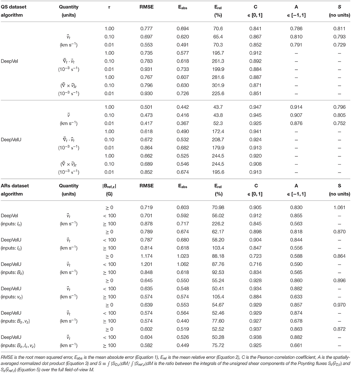
Table 1. Comparison between the 30-timestep-averaged ${\overrightarrow{v}}_{\text{D},t}$ and ${\overrightarrow{v}}_{\text{ref},t}$ for the QS dataset and ARs dataset.

FIGURE 1

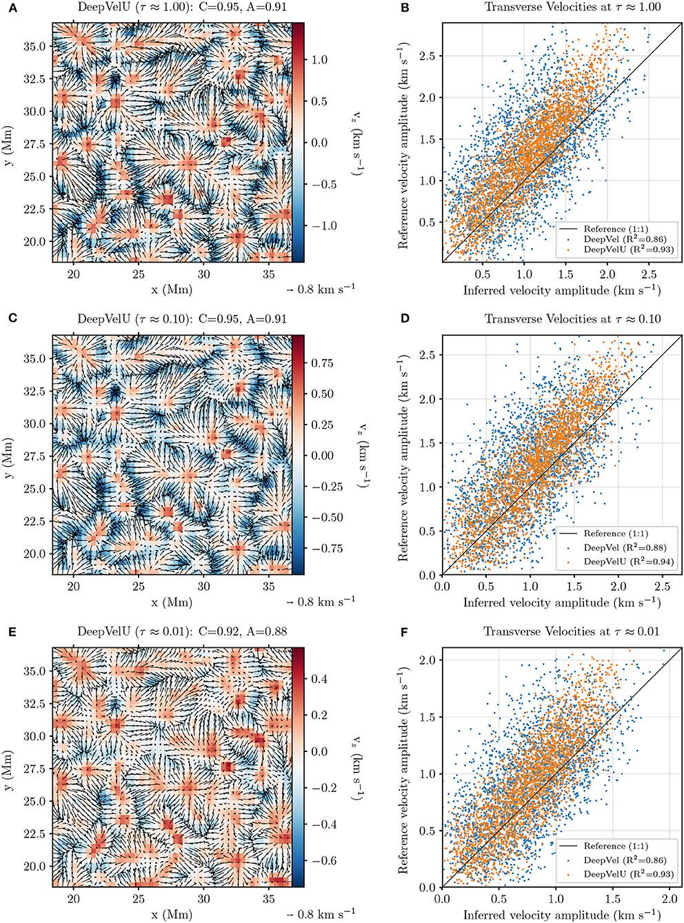
Figure 1. (Left) Patches of 50 by 50 pixels² extracted from the 30-timestep-averaged transverse velocity fields ${\overrightarrow{v}}_{D,t}$ inferred by DeepVelU at optical depths (A) τ ≈ 1, (C) τ ≈ 0.1, and (E) τ ≈ 0.01. The 30-timestep-averaged vertical velocity v_{z, ref}(τ ≈ {1, 0.1, 0.01}) computed by the STAGGER simulation and resampled to the SDO/HMI resolution is displayed as background (colorscale). (Right) Scatterplots comparing amplitudes $\left|{\overrightarrow{v}}_{\text{D},t}\right|$ to $\left|{\overrightarrow{v}}_{\text{ref},t}\right|$ at optical depths (B) τ ≈ 1, (D) τ ≈ 0.1, and (F) τ ≈ 0.01. The black line represents the expected solution (i.e., a coefficient of determination R² = 1).

Similar conclusions are drawn for the inversion of flows at optical depths τ ≈ {0.1, 0.01} (i.e., at higher geometrical heights above the surface) from I_c(τ ≈ 1) (Figure 1 and Table 1). More specifically, τ ≈ 0.1 is just beyond the height where the reversal of the granulation pattern occurs (i.e., a few hundred kilometers above the surface: Cheung et al., 2007), with the center of granules becoming colder than the intergranular network. At τ ≈ 0.01, this pattern is more diffused but remains well-correlated with the surface granulation pattern (not shown). By extension, the structures in ${\overrightarrow{v}}_t(\tau \approx \left\{0.1,0.01\right\})$ correlate with I_c(τ ≈ 1).

The power spectrum of the kinetic energy (Equation 4) as a function of the spatial scales shows an improved response for DeepVelU at supergranular scales (k⁻¹ ≈ 100 Mm) with respect to the test set (green and blue curves in Figure 2A). The transition from a loss to a gain in signal with respect to DeepVel (orange curve) occurs close to the spatial scale that is achieved through downsampling at the bottleneck of the U-net architecture (k⁻¹ ≈ 2.944 Mm). This change is interpreted as the new architecture favoring signal at supergranular scales over the pixel-size and granular scales to further optimize the cost function during the training process.

FIGURE 2

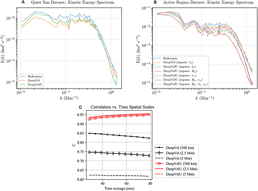
Figure 2. Power spectra of the total kinetic energy E(k) of the 30-timestep averaged transverse velocities as a function of the wavenumber k. (A) QS dataset. (B) ARs dataset. (C) Pearson correlation between the simulated transverse velocity field in the QS as a function of time and spatial averaging windows. The latter is shown with the full width at half maximum of the Gaussian kernel used.

In addition, Figure 2C shows a significant improvement for DeepVelU in the correlation between the inferred velocities and the simulation at all time and spatial scales for the QS. DeepVel's flows have the surprising disadvantage of losing correlation at increasing time averages by a few percents, whereas the correlation increases for DeepVelU. Similarly, DeepVel's correlations significantly decreases at greater spatial averages, e.g., from (resp.) C ≈ 0.85 to C ≈ 0.62 between 368 km and 5 Mm (resp.), which is not the case for DeepVelU which consistently correlates very well with the simulation at C > 0.9. The latter, however, plateaus near 3 Mm which coincides with the pixel-size in the bottleneck of the U-net architecture. Future work will test if increasing the field-of-view of the training images affects favorably the ability to improve the correlation further at greater spatial scales.

3.3. Active Region Test Set

Figures 3A,C,E show a subset of velocity field inversions generated by DeepVelU from single-quantity inputs that relate to SDO/HMI level-2 data products i.e., intensitygrams, line-of-sight magnetograms,and Dopplergrams, respectively. Only a sub-field of 50 by 50 pixels² is shown for clarity. The position of this patch in the field-of-view was selected to highlight distinct flow structures in the presence of ARs: the center of the sunspot (upper right corner), the flows in the penumbra, the moat-like flows around the latter (close to the diagonal connecting the upper left corner to the lower right corner), and finally, the granulation like in the QS dataset (lower left corner). Scatterplots in Figure 3 were computed over the sub-field whereas the metrics compiled in Table 1 were computed over the entire field-of-view and include all tested combinations of inputs. An arbitrary threshold of |B_{ref, z}| ≥ 100 G is set to compute metrics that are specific to the AR and the magnetic field network. Regions where |B_{ref, z}| < 100 G are interpreted as QS.

FIGURE 3

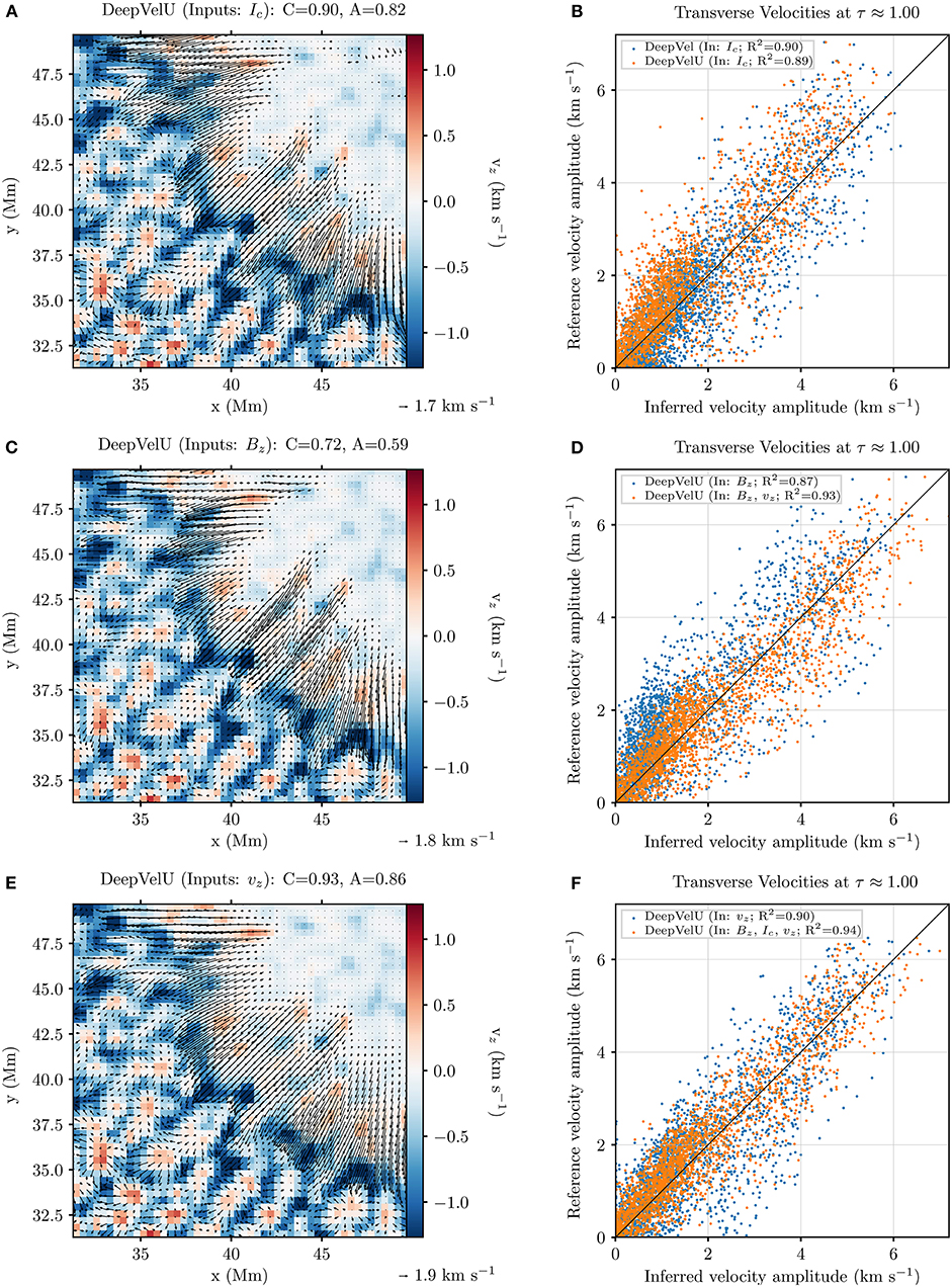
Figure 3. (Left) Patches of 50 by 50 pixels² extracted from the 30-timestep-averaged ${\overrightarrow{v}}_{D,t}(\tau \approx 1)$ inferred by DeepVelU from (A) I_c(t = t_i, t_i + Δt), (C) B_z(t = t_i, t_i + Δt), and (E) v_z(t = t_i, t_i + Δt). The 30-timestep-averaged v_{z, ref} computed by the MURaM simulation and resampled to the SDO/HMI resolution is displayed as background (colorscale). (Right) Scatterplots comparing $\left|{\overrightarrow{v}}_{\text{ref},t}\right|$ to $\left|{\overrightarrow{v}}_{D,t}\right|$ inferred from a combination of intensitygrams I_c(t = t_i, t_i + Δt), magnetograms B_z(t = t_i, t_i + Δt) and Dopplergrams v_z(t = t_i, t_i + Δt). The black line represents the expected solution (i.e., R² = 1). (Right) Scatterplots comparing $\left|{\overrightarrow{v}}_{\text{ref},t}\right|$ to $\left|{\overrightarrow{v}}_{\text{ref},t}\right|$ inferred from a combination of (B) consecutive intensitygrams I_c(t = {t_i, t_{i + Δt}}), (D) magnetograms B_z(t = {t_i, t_{i + Δt}}) and Dopplergrams v_z(t = {t_i, t_{i + Δt}}), and (F) Dopplergrams, intensitygrams and magnetograms.

DeepVel and DeepVelU generate very similar velocity fields from consecutive intensitygrams, with DeepVel performing slightly better where |B_{ref, z}| < 100 G and DeepVelU (Figure 3A) improving absolute and relative errors slightly where |B_{ref, z}| ≥ 100 G (Table 1) but underestimating low amplitude velocities (Figure 3B). In fact, the performances of the two neural networks are comparable to that of DeepVel with the QS dataset (Table 1). For both architectures, the signal for the continuum intensity inside the Sunspot results in less effective flow inversions where |B_{ref, z}| ≥ 100 G. More specifically, the mean relative error almost doubles when transitioning from the QS to strong field regions and the metric A describing the global orientation of the vectors decreases to a value of about 0.55 (Table 1). For this reason, different combinations of physical inputs were tested to measure their impact on photospheric flows. Although these tests were performed using the DeepVelU architecture, we expect that similar conclusions can be drawn for the DeepVel neural network.

The use of line-of-sight magnetograms as inputs instead of intensitygrams slightly improves the errors where |B_{ref, z}| ≥ 100 G (Table 1), i.e., where there is the most signal in the input data. Despite weak magnetic fields in the QS, the neural network is capable of distinguishing individual granules and their flow patterns (Figure 3C), but the errors are significantly larger with greatly underestimated flow amplitudes (Figure 3D) and misaligned vectors (Table 1). The overall performance is thus worse due to a larger fraction of the field-of-view being covered by QS (Table 1).

Dopplergrams, such as the ones depicted in the background of Figures 3A,C,E, are the inputs that best capture the behavior of flows in both QS and ARs (Table 1 and Figure 3F). The granulation pattern from intensitygrams is clearly outlined in Dopplergrams by the cold sinking plasma in the intergranular lanes and the hot rising plasma at the center of granules. Meanwhile convective motions are inhibited inside Sunspots. However, flows in the penumbra are predicted by DeepVelU to be almost purely radial with respect to the center of the Sunspot (Figure 3E), whereas the simulation penumbral flows resemble more closely those seen in Figures 3A,C. Although the metric A was slightly improved in strong field regions, vector orientations remain much less accurately reproduced than in the QS (Table 1).

Combining B_{ref, z} and v_{ref, z}, which yielded the best reconstructions for ARs and QS, respectively, significantly improves the performance for ARs and the integrated Poynting flux (Table 1). Magnetograms provide to Dopplergrams additional signal inside Sunspots. Both quantities are coupled physically to ${\overrightarrow{v}}_t$ through the magnetic induction equation, which could further explain the increase in performance. The addition of intensitygrams provides more context for the QS and improves the metrics where |B_{ref, z}| < 100 G, with very little to no decrease in performance where |B_{ref, z}| ≥ 100 G (Table 1).

The use of Dopplergrams or combinations of inputs in DeepVelU improves the response in the power spectrum of the kinetic energy for spatial scales larger than k⁻¹ ≈ 3 Mm (Figure 2B), which could again be related to the spatial scales probed in the U-net's bottleneck. Although the power is generally underestimated, its variations as a function of k are matched more consistently by DeepVelU, with DeepVel generating more signal than the simulation at supergranular scales.

4. Conclusion

We trained DeepVelU, a U-net-inspired architecture for the DeepVel neural network, using simulations of the QS and ARs and evaluated the method's response as a function of spatial and temporal scales. DeepVelU shows significant improvement over DeepVel for the QS test set. The correlations for the latter falls close to 0.6 at spatial scales of 5 Mm whereas it stays consistently above 0.9 for DeepVelU; increasing at greater time averages and plateauing at spatial scales above 3 Mm. Thus DeepVelU's QS model appears more effective than the other tracking methods tested in Tremblay et al. (2018) against the same dataset, with increased correlations and lower errors being achieved over DeepVel at granular scales and over FLCT at supergranular scales. The results for the ARs dataset are not as conclusive, but may be further improved by training for granulation, penumbra and sunspots separately. This approach could, however, introduce discontinuities at the edges of the different structures.

Current efforts are meant to be a proof of concept. Limitation of the method include the input image dimensions in each direction which must be a factor of 2ⁿ where n is the number of downsampling or upsampling layers in the network architecture (here n = 3). For example, the dimensions of the sub-images (48 × 48 px²) presented to the network during training limited the number of downsampling/upsampling layers in the architecture to n = 3, corresponding to a spatial of about 3 Mm. This could explain the plateauing of the correlation above this spatial scale. In this context, development is underway for a deeper version of DeepVelU (i.e., with more downsampling/upsampling layers) that will be trained on (almost) full field-of-view images (256 × 256 px² or 94.192 × 94.192 Mm²) of the QS dataset and that will also double (resp. halve) the number of filters after each downsampling (resp. upsampling) operation. In addition, the simulations do not model actual supergranulation which is known to advect granules over spatial scales greater than 3 Mm. Therefore it will be worth exploring further inferences on actual photospheric observations. For example we plan to compare the inferred supergranular (QS) and moat flow patterns (ARs) with those of Attie et al. (2018) which uses a new implementation of the “Balltracking” method that is more accurate than the one of Potts et al. (2004) and that had not been tested by Tremblay et al. (2018). Similarly, the MURaM simulation includes a deep seated flow system with velocities in the 200–500 m/s range which extends about 10 Mm past the sunspot boundary, which seems in line with many observations of moat flows (Rempel, 2015). Using the data of both experiments (observations and simulation), we will compare the moat flow patterns revealed by DeepVel, DeepVelU and Balltracking.

The inclusion of Dopplergrams and line-of-sight magnetograms as inputs in the neural network architecture, both of which provide more signal than intensitygrams inside sunspots and are tied to the transverse plasma motions through the magnetic induction equation, have improved reconstructions in the context of ARs and response at supergranular scales. Evaluating the impact of additional inputs such as the transverse magnetic field vector ${\overrightarrow{B}}_t$ which also appears in the magnetic induction equation or its strength $\left|{\overrightarrow{B}}_t\right|$ which is not subjected to ambiguities is left as future work.

Despite the changes in architecture and the success of the neural network at capturing the spatial distribution of flows, velocity amplitudes are generally underestimated in the QS and overestimated in ARs by both DeepVel and DeepVelU. Future efforts will be dedicated to improving the inferral of amplitudes.

All versions of the neural networks were trained to generate synthetic data that is consistent with a given simulation and the SDO/HMI cadence (if the velocity is multiplied by a factor of 45/60 for the QS dataset) and spatial resolution near disk center. SDO/HMI level-2 products can thus be used as input, however one should first assess if the physics and preprocessing of the training set is consistent with the observations presented as input. For instance, SDO/HMI Dopplergrams measure the superposition of the line-of-sight components of the satellite motion, meridional flows, differential rotation, p-mode oscillations, and plasma motions. Simulation Dopplergrams only feature the latter two. Additional preprocessing steps are thus required to correct SDO/HMI Dopplergrams for the aforementioned effects (e.g., Welsch et al., 2013) or to project the simulation data in the observations space prior to training. The resulting velocity fields may then serve as synthetic observations or first estimates when performing data assimilation in an MHD model of the photosphere, or as boundary conditions driving a simulation. The method may also be used to estimate and evolve a Poynting flux vector that is representative of a given epoch of the Sun.

The velocity vector that the neural networks are trying to recover is the same vector as physics-based velocity inversion methods, i.e., ${\overrightarrow{v}}_t$ such that the magnetic induction equation is satisfied. Furthermore, DeepVelU best performed when using Dopplergrams and magnetograms as input, with both quantities appearing in the magnetic induction equation alongside $\overrightarrow{v}$. The training process may be revisited in the future to incorporate more effectively the physics when estimating the plasma motions, e.g., through the loss function or a physics-informed network (Raissi et al., 2019).

Data Availability Statement

The QS and ARs weights and biases as well as the DeepVel and DeepVelU outputs generated and analyzed for this study can be found in the DeepVelU_Frontiers repository (https://github.com/tremblaybenoit/DeepVelU_Frontiers).

Author Contributions

BT generated the QS and ARs datasets from simulation data. BT also trained and tested all versions of the DeepVel and DeepVelU neural networks. RA acquired the ARs dataset prior to BT downsampling the data to the SDO/HMI spatial resolution. RA also provided the analysis of the QS dataset.

Conflict of Interest

The authors declare that the research was conducted in the absence of any commercial or financial relationships that could be construed as a potential conflict of interest.

Acknowledgments

The authors would like to thank Prof. Laurence Perreault-Levasseur (MILA; Université de Montréal) for her advice regarding the neural network architecture. The authors would also like to thank Prof. Maria Kazachenko for her insight and her advice during the writing of this manuscript. The MURaM simulation data was kindly provided by Dr. Matthias Rempel (NCAR).

Footnotes

1. ^DeepVel is an open-source neural network: https://github.com/aasensio/deepvel.

2. ^Computations performed by the STAGGER code are available for download: http://steinr.pa.msu.edu/~bob/96averages/.

References

Abbett, W. P., and Fisher, G. H. (2010). Improving large-scale convection-zone-to-corona models. Memorie della Societa Astronomica Italiana 81:721. Available online at: https://www.adsabs.harvard.edu/abs/2010MmSAI.81.721A

Google Scholar

Asensio Ramos, A., Requerey, I. S., and Vitas, N. (2017). DeepVel: deep learning for the estimation of horizontal velocities at the solar surface. Astron. Astrophys. 604:A11. doi: 10.1051/0004-6361/201730783

CrossRef Full Text | Google Scholar

Attie, R., Innes, D. E., and Potts, H. E. (2009). Evidence of photospheric vortex flows at supergranular junctions observed by FG/SOT (Hinode). Astron. Astrophys. 493, L13-L16. doi: 10.1051/0004-6361:200811258

CrossRef Full Text | Google Scholar

Attie, R., Innes, D. E., Solanki, S. K., and Glassmeier, K. H. (2016). Relationship between supergranulation flows, magnetic cancellation and network flares. Astron. Astrophys. 596:A15. doi: 10.1051/0004-6361/201527798

CrossRef Full Text | Google Scholar

Attie, R., Kirk, M. S., Thompson, B. J., Muglach, K., and Norton, A. A. (2018). Precursors of magnetic flux emergence in the moat flows of active region ar12673. Space Weather 16, 1143–1155. doi: 10.1029/2018SW001939

CrossRef Full Text | Google Scholar

Cheung, M. C. M., Schüssler, M., and Moreno-Insertis, F. (2007). The origin of the reversed granulation in the solar photosphere. Astron. Astrophys. 461, 1163–1171. doi: 10.1051/0004-6361:20066390

CrossRef Full Text | Google Scholar

Fisher, G. H., Abbett, W. P., Bercik, D. J., Kazachenko, M. D., Lynch, B. J., Welsch, B. T., et al. (2015). The coronal global evolutionary model: using HMI vector magnetogram and doppler data to model the buildup of free magnetic energy in the solar corona. Space Weather 13:369. doi: 10.1002/2015SW001191

CrossRef Full Text | Google Scholar

Fisher, G. H., and Welsch, B. T. (2008). “FLCT: a fast, efficient method for performing local correlation tracking,” in Subsurface and Atmospheric Influences on Solar Activity, Volume 383 of Astronomical Society of the Pacific Conference Series, eds R. Howe, R. W. Komm, K. S. Balasubramaniam, and G. J. D. Petrie (San Francisco, CA), 373.

Google Scholar

Hagenaar, M. (2005). “Photospheric surface flows and sunspot moats,” in Large-Scale Structures and Their Role in Solar Activity, Volume 346 of Astronomical Society of the Pacific Conference Series, eds K. Sankarasubramanian, M. Penn, and A. Pevtsov (San Francisco, CA), 41.

Google Scholar

Hoeksema, J. T., Liu, Y., Hayashi, K., Sun, X., Schou, J., Couvidat, S., et al. (2014). The helioseismic and magnetic imager (HMI) vector magnetic field pipeline: overview and performance. Sol. Phys. 289, 3483–3530. doi: 10.1007/s11207-014-0516-8

PubMed Abstract | CrossRef Full Text | Google Scholar

Illarionov, E. A., and Tlatov, A. G. (2018). Segmentation of coronal holes in solar disc images with a convolutional neural network. Monthly Notices R. Astron. Soc. 481, 5014–5021. doi: 10.1093/mnras/sty2628

CrossRef Full Text | Google Scholar

Ioffe, S., and Szegedy, C. (2015). “Batch normalization: accelerating deep network training by reducing internal covariate shift,” in Proceedings of the 32nd International Conference on International Conference on Machine Learning, Vol. 37 (Lille: JMLR), 448–56. doi: 10.5555/3045118.3045167

CrossRef Full Text | Google Scholar

Kazachenko, M. D., Fisher, G. H., and Welsch, B. T. (2014). A comprehensive method of estimating electric fields from vector magnetic field and Doppler measurements. Astrophys. J. 795:17. doi: 10.1088/0004-637X/795/1/17

CrossRef Full Text | Google Scholar

Kazachenko, M. D., Fisher, G. H., Welsch, B. T., Liu, Y., and Sun, X. (2015). Photospheric electric fields and energy fluxes in the eruptive active region NOAA 11158. Astrophys. J. 811:16. doi: 10.1088/0004-637X/811/1/16

CrossRef Full Text | Google Scholar

Liu, Y., and Schuck, P. W. (2012). Magnetic energy and helicity in two emerging active regions in the sun. Astrophys. J. 761:105. doi: 10.1088/0004-637X/761/2/105

CrossRef Full Text | Google Scholar

Longcope, D. W. (2004). Inferring a photospheric velocity field from a sequence of vector magnetograms: the minimum energy fit. Astrophys. J. 612, 1181–1192. doi: 10.1086/422579

CrossRef Full Text | Google Scholar

November, L. J., and Simon, G. W. (1988). Precise proper-motion measurement of solar granulation. Astrophys. J. 333, 427–442. doi: 10.1086/166758

CrossRef Full Text | Google Scholar

Potts, H. E., Barrett, R. K., and Diver, D. A. (2004). Balltracking: an highly efficient method for tracking flow fields. Astron. Astrophys. 424, 253–262. doi: 10.1051/0004-6361:20035891

CrossRef Full Text | Google Scholar

Potts, H. E., and Diver, D. A. (2008). Automatic recognition and characterisation of supergranular cells from photospheric velocity fields. Sol. Phys. 248, 263–275. doi: 10.1007/s11207-007-9068-5

CrossRef Full Text | Google Scholar

Raissi, M., Perdikaris, P., and Karniadakis, G. E. (2019). Physics-informed neural networks: a deep learning framework for solving forward and inverse problems involving nonlinear partial differential equations. J. Comput. Phys. 378, 680–707. doi: 10.1016/j.jcp.2018.10.045

CrossRef Full Text | Google Scholar

Rempel, M. (2015). Numerical simulations of sunspot decay: on the penumbra-evershed flow-moat flow connection. Astrophys. J. 814:125. doi: 10.1088/0004-637X/814/2/125

CrossRef Full Text | Google Scholar

Rempel, M., and Cheung, M. C. M. (2014). Numerical simulations of active region scale flux emergence: from spot formation to decay. Astrophys. J. 785:90. doi: 10.1088/0004-637X/785/2/90

CrossRef Full Text | Google Scholar

Rieutord, M., and Rincon, F. (2010). The sun's supergranulation. Living Rev. Solar Phys. 7, 16–17. doi: 10.12942/lrsp-2010-2

CrossRef Full Text | Google Scholar

Rieutord, M., Roudier, T., Ludwig, H.-G., Nordlund, Å., and Stein, R. (2001). Are granules good tracers of solar surface velocity fields? Astron. Astrophys. 377, L14-L17. doi: 10.1051/0004-6361:20011160

CrossRef Full Text | Google Scholar

Rieutord, M., Roudier, T., Rincon, F., Malherbe, J.-M., Meunier, N., Berger, T., et al. (2010). On the power spectrum of solar surface flows. Astron. Astrophys. 512:A4. doi: 10.1051/0004-6361/200913303

CrossRef Full Text | Google Scholar

Rieutord, M., Roudier, T., Roques, S., and Ducottet, C. (2007). Tracking granules on the Sun's surface and reconstructing velocity fields. I. The CST algorithm. Astron. Astrophys. 471, 687–694. doi: 10.1051/0004-6361:20066491

CrossRef Full Text | Google Scholar

Ronneberger, O., Fischer, P., and Brox, T. (2015). U-Net: convolutional networks for biomedical image segmentation. arXiv preprints arXiv:1505.04597. doi: 10.1007/978-3-319-24574-4_28

CrossRef Full Text | Google Scholar

Schou, J., Scherrer, P. H., Bush, R. I., Wachter, R., Couvidat, S., Rabello-Soares, M. C., et al. (2012). Design and ground calibration of the helioseismic and magnetic imager (HMI) instrument on the solar dynamics observatory (SDO). Sol. Phys. 275, 229–259. doi: 10.1007/s11207-011-9842-2

PubMed Abstract | CrossRef Full Text | Google Scholar

Schuck, P. W. (2005). Local correlation tracking and the magnetic induction equation. Astrophys. J. Lett. 632, L53-L56. doi: 10.1086/497633

CrossRef Full Text | Google Scholar

Schuck, P. W. (2006). Tracking magnetic footpoints with the magnetic induction equation. Astrophys. J. 646, 1358–1391. doi: 10.1086/505015

CrossRef Full Text | Google Scholar

Schuck, P. W. (2008). Tracking vector magnetograms with the magnetic induction equation. Astrophys. J. 683, 1134–1152. doi: 10.1086/589434

CrossRef Full Text | Google Scholar

Sheeley, N. R. J. (1969). The evolution of the photospheric network. Sol. Phys. 9, 347–357. doi: 10.1007/BF02391657

CrossRef Full Text | Google Scholar

Stein, R. F. (2012). Solar surface magneto-convection. Living Rev. Sol. Phys. 9:5. doi: 10.12942/lrsp-2012-4

PubMed Abstract | CrossRef Full Text | Google Scholar

Stein, R. F., and Nordlund, Å. (2012). On the formation of active regions. Astrophys. J. Lett. 753:L13. doi: 10.1088/2041-8205/753/1/L13

CrossRef Full Text | Google Scholar

Tremblay, B., Roudier, T., Rieutord, M., and Vincent, A. (2018). Reconstruction of horizontal plasma motions at the photosphere from intensitygrams: a comparison between DeepVel, LCT, FLCT, and CST. Sol. Phys. 293:57. doi: 10.1007/s11207-018-1276-7

CrossRef Full Text | Google Scholar

Wachter, R., Schou, J., Rabello-Soares, M. C., Miles, J. W., Duvall, T. L., and Bush, R. I. (2012). Image quality of the helioseismic and magnetic imager (HMI) onboard the solar dynamics observatory (SDO). Sol. Phys. 275, 261–284. doi: 10.1007/s11207-011-9709-6

CrossRef Full Text | Google Scholar

Welsch, B. T. (2015). The photospheric Poynting flux and coronal heating. Publ. Astron. Soc. Japan 67:18. doi: 10.1093/pasj/psu151

CrossRef Full Text | Google Scholar

Welsch, B. T., Fisher, G. H., and Sun, X. (2013). A magnetic calibration of photospheric Doppler velocities. Astrophys. J. 765:98. doi: 10.1088/0004-637X/765/2/98

CrossRef Full Text | Google Scholar