Spectral Deconvolution With Deep Learning: Removing the Effects of Spectral PSF Broadening

1. Introduction

The finite spectral resolution of real instruments affects the inferred signal by blending the intensities at different wavelengths. This phenomenon is problematic for (solar) spectral lines, since the shape of a line encodes essential information about a range of heights in the solar atmosphere. However, some instruments use a lower spectral resolution (broader spectral transmission profile) to increase instrument throughput and reduce integration times. Such a broad spectral point-spread function (sPSF) results fundamentally in a multiplexed sampling of the line profile, with the information from a given portion of the original spectral profile sampled multiple times at various positions in the sPSF (i.e., with varying relative attenuation) as the transmission function is tuned through the line. This means that it should be possible to recover much of the underlying spectral information from this linear combination of samplings. The concept of exploiting this multiplexing to recover spectral information was originally developed by Caccin and Roberti (1979) and later Baranyi and Ludmány (1983) in order to reconstruct spectral profiles sampled by the relatively broad (0.15–0.5 Å FWHM) sPSF of the tunable Universal Birefringent Filter (UBF) (Beckers et al., 1975). The method developed, which relied on analytical descriptions of the sPSF, was employed by Caccin et al. (1983) and Baranyi (1986) to reconstruct H-alpha and Na D line profiles recorded through a UBF. However, the data at the time were recorded on photographic film and the method was sensitive to noise and computationally demanding. The current observational demands for high-resolution imaging have resulted in instruments based on Fabry-Pérot-interferometers that have sPSF's that are again suitable for this method.

In this work, we seek to evaluate machine-learning techniques that can retrieve higher-resolution spectra from instrumentally broadened spectral profiles. The effect of spectral smearing on the line shape is shown in the left panel of Figure 1 with an example spectrum of Ca II 8,542 Å from the FISS/BBSO (Chae et al., 2013) spectrograph. The orange line is the spectrum as observed with the full spectral resolution of FISS of about R~150,000 (where spectral resolution R is defined as the wavelength of observation divided by the FWHM of the profile). Instead, the blue line shows the same spectrum convolved with a Lorentzian-shaped sPSF with R~45,000. Given the typical shape of an absorption line, the convolution with a broad sPSF raises the intensity around the line core and broadens the wings of the profile.

FIGURE 1

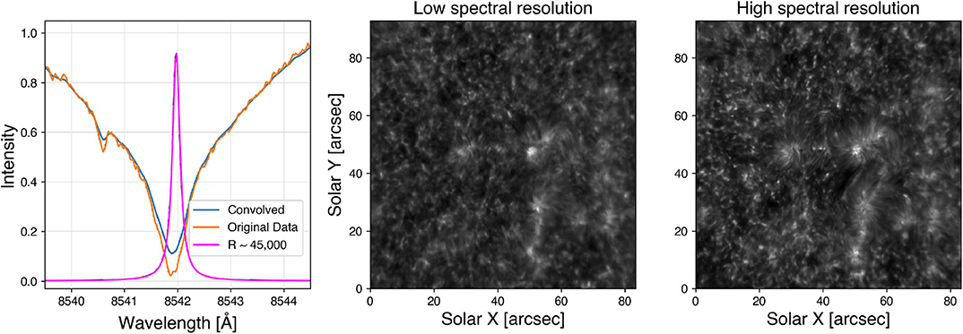
Figure 1. (Left) Comparison of a sample line profile of the Ca II 8,542 Å line from the FISS dataset described in section 3 before ($\text{orange}$) and after ($\text{blue}$) convolution with the sPSF ($\text{magenta}$); The $\text{magenta}$ curve is the transmission profile used for convolving the orange profile to get the blue one (corresponding to FP 2 of IBIS with R~45,000); (Center and Right) Comparison of chromospheric quiet Sun region observed with IBIS with low spectral resolution (R~50,000) on the central panel and with high spectral resolution (R~200,000) in the right panel.

This smearing tends to increase the similarity among different spectral profiles, also reducing the spatial contrast and the ability to identify small scale structures in images of the solar atmosphere. An example of this is presented in Figure 1 (central and right panels), with observations in the core of the Ca II 8,542 Å line from the Interferometric Bidimensional Spectrometer (IBIS) (Cavallini, 2006) instrument at the Dunn Solar Telescope The same FOV was observed at the instrument's normal high spectral resolution (R~200,000), but also at a much lower spectral resolution (R~50,000), which was achieved by removing the “narrow passband” Fabry-Pérot interferometer (FPI) from the optical path (Reardon and Cavallini, 2008). We can see the reduced contrast in the FOV with lower spectral resolution which deteriorates the identification of the chromospheric features. Hence, mitigation of the degraded spectral purity of our observations is essential for furthering our understanding of the Sun.

Furthermore, the compressible nature of spectral lines as suggested by allow the sampling and subsequent recovery of the full spectral profiles with a lesser number of measurements by using a suitably adopted measurement basis. This approach could improve instrumental performance by increasing the sampling cadence through a reduction in the number of instrumental tuning steps needed to sample the line.

In this paper we perform experiments to test the applicability of Convolutional Neural Networks (CNNs) to perform the de-multiplexing of spectral line profiles in different scenarios. We examine the photometric accuracy than can be achieved with these techniques. Finally, we discuss the limitations on the precision of the recovered profiles based on the dimensionality of the data derived from maximum-likelihood intrinsic-dimensionality estimate (Levina and Bickel, 2004).

2. A Deep Learning Approach

We utilize deep Convolutional Neural Networks (CNNs) for the deconvolution process as they are powerful function approximators which are widely used for pattern recognition and image processing (Goodfellow et al., 2016). We used an encoder-decoder architecture because it can extract the relevant features from noisy data (encoder) and then recreate the signal of interest from the latent space (decoder). The architecture of the network consists of three convolutional layers, followed by three symmetric upsampling (“deconvolutional”) layers, followed by two dense layers with dimensions of the output data. The three consecutive convolutional layers (and their corresponding upscaling layers) have [5, 10, 20] filters and used a three-pixel kernel. Rectified Linear unit (RELU) activation function was used for all layers with the exception of the last one where we have used a linear activation function (He et al., 2016). Furthermore, in section 3 we add the input layer to the last dense layer of the network to improve the performance of the network. This is due to the fact that in this architecture, the network has to estimate only the corrections to the convoluted signal instead of recreating the whole spectral line profile. However, this will cause the core of the spectral profile to be poorly fit since the most significant corrections are needed there (as can be seen in left panel of Figure 1). To alleviate this issue, we introduce a custom loss function which is a weighted mean square error. The weights are chosen inversely proportional to the intensity of the line profile so as to emphasize the precision of the recovered profiles in the line core. We trained our network with the Adam optimizer (Kingma and Ba, 2014) for about one thousand epochs before satisfactory convergence was achieved. The network was implemented with Keras under Tensorflow (Abadi et al., 2015) and can be found in the public repository of the project.

3. Spectral Deconvolution With CNN

3.1. Deconvolution of Synthetic Data From FISS

To test the CNN approach for sPSF deconvolution, we utilized Ca II 8,542 Å data from the FISS/BBSO (Chae et al., 2013) instrument (R~150,000) obtained on June 22, 2016. We created a training set by convolving each spectral profile with a Lorentzian sPSF with an effective R ~ 45,000 [corresponding roughly to the FWHM of IBIS's FPI #2 transmission profile (Reardon and Cavallini, 2008)]. The bottom left panel of Figure 2 shows a sample profile from the FISS instrument in blue and convolved with the FPI #2 profile in green. The CNN was trained with spectra from a single raster scan 100 × 250 spatial pixels corresponding to 16 × 20 arcseconds on the Sun centered on a pore near disk center which took 16.5 s. Satisfactory convergence was accomplished in about 1,000 epochs with the relative RMS error at the last epoch of the training reaching about 1.5 × 10⁻⁴.

FIGURE 2

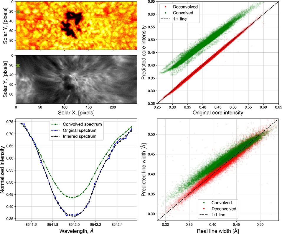
Figure 2. (Top left) Continuum image/Line core intensity of Ca II 8542 Å of the FISS dataset used for the experiment in sections 3.1 and 4; (Bottom left) A sample profile (coordinates [4, 21] in our datacube, green cross in top left panel) shown before convolution with wide SPSF ($\text{blue line}$), after the convolution ($\text{green}$) and after the deconvolution with the CNN (black); (Top right) Comparison of the line core intensity recovered with the algorithm—true line profile (black line is the one-to-one line). The approach for measuring line intensity and width are described in section 3.1. (Bottom right) Same as the previous panel but for the line core width of the Ca II 8,542 Å line.

The performance of the CNN was tested on a different raster (data not seen by the network previously) from FISS of the same region of the Sun acquired 5 minutes after the scan used for training. The line core intensity value and position was determined as the minimum of a parabola fitted to the 7 points around the pixel position with the lowest intensity. The core width of the line profile was measured (following Cauzzi et al., 2009) as the bisector width at the intensity equal to half the difference between intensity of the line core and the intensity at a fixed offset of 0.4 Å from the wavelength position of the line core.

The algorithm achieved 0.76% precision photometry of the line core intensity and 2.5% precision retrieving the line core width. These results are illustrated in the right column of Figure 3. This example shows the robustness of the ML approach for retrieving spectral line profiles. The algorithm takes about 7 × 10⁻⁶ s for a single inversion of 40 point spectrum on an Intel i7-4780HQ CPU and only 0.3 × 10⁻⁶ s on a NVIDIA TITAN RTX GPU. We take into account the I/O overhead for the GPU inversions, as we used a dataset of 16 million spectra with 40 wavelengths points (similar to the VTF full CCD readout) which amounts to about 20% of the memory of the GPU. This method is slightly faster than the scipy.signal.deconvolve algorithm which uses a digital filter, but the latter cannot reproduce the wings of the line well due to boundary effects. Compared to more computationally intensive algorithms such as the Richardson-Lucy (Richardson, 1972) deconvolution algorithm, we found that our algorithm is about 100 times faster. Furthermore, it does not require fine tuning of parameters once a suitable training set is provided.

FIGURE 3

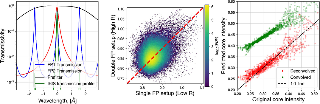
Figure 3. (Left) Transmission profile of the components of the IBIS Instrument centered around 8,542 Å. The transmission profiles of the two Fabry-Pérot etalons are in $\text{red}$ and $\text{blue}$; the 8,542 Å prefilter profile is the black line; The effective transmission profile of the instrument is presented in $\text{green}$; (Center) Histogram of the wing intensity in the data sets with single FP (low R) and both FPs (high R) in the optical system; (Right) The result of the deconvolution algorithm applied to real IBIS data (same as top right panel in Figure 2) for the line core intensity.

3.2. Deconvolution of Real Spectral Data From IBIS

To test the method on real Fabry-Pérot data we obtained a dataset with the IBIS instrument at the DST with high (R ~ 200,000) and low (R ~ 50,000, similar to the FISS tests above) spectral resolution of the same region of the Sun. We achieved the different spectral resolutions by utilizing the fact that the IBIS instrument consists of two Fabry-Pérot (FP) interferometers in series, one of which has a profile three times narrower than the other (the components of the IBIS instrument are presented in the left panel of Figure 3). Hence, if we take the narrower FP (FP #1) out of the optical path, we obtain observations with a lower spectral resolution. We imaged a region near disk center of the Sun in the Ca II 8,542 Å line, where we scanned a spectral region of 4.4 Å centered around the line core with a spacing of 50 mÅ. We acquired five separate exposures at each wavelength [for post-processing MOMFBD (van Noort et al., 2005) reconstruction to minimize seeing effects] which resulted in two datasets of the same solar structures with different spectral resolution taken 4 minutes apart. We applied the deconvolution algorithm to the these datasets using as the input the lower spectral resolution data obtained with a single FP and as the expected output the higher spectral resolution dataset obtained with both FPs. Images from the two datasets are presented in the central and right panels of Figure 1.

We had limited success with deconvolving this dataset as the spectral profiles had changed significantly even over the 4 minute interval between the datasets. To illustrate this, the central panel of Figure 3 shows the density plot of the quasi-continuum in the wings of the two datasets. The lack of obvious correlation (confirmed by visual inspection of the data) shows that the structures on the solar surface have significantly changed between the two datasets were obtained (consistent with granular lifetimes of ~8 minutes).

To explore the validity of this deconvolution approach, we chose a subset of spatial pixels from the IBIS scans based on certain criteria to identify spectral profiles that did not change significantly between the two samplings. This step allows the CNN to train primarily on the effects from the spectral smearing, not the evolution of the solar atmosphere. The imposed criteria are that the measured Doppler velocity change¹ between the two consecutive samplings is no greater than half a resolution element (0.6 km/s) and that the location of the pixel in the cumulative distribution of intensity and width (relative to the other pixels sampled at the same spectral resolution) does not change by more than 5 percentiles. The expected vs. deconvolved core intensities are presented in the right panel of Figure 3 (compare to Figure 2). The scatter is larger than the FISS synthetic data due to the effects of solar surface evolution occurring between the acquisition of the two components of the training set, whose correction is beyond the scope of this project. Future tests of this method could emphasize obtaining a more nearly cotemporal training dataset by restricting the range of the spectral scan around line core, reducing the time separation between the different spectral resolution scans significantly. We note that distinct training datasets, derived at different times or even using a separate instrument (e.g., a slit spectrograph), could be applied to multiple datasets obtained with a low-spectral-resolution FP instrument [e.g., VTF (Kentischer et al., 2012) at the DKIST (Tritschler et al., 2016)], under the assumption that: (a) the sPSF and straylight of each instrument is well characterized; and (b) the same general types of solar spectral profiles are sampled in both cases.

4. Recovering Undersampled Spectral Profiles With Multi-Peaked sPSF

It was suggested by Asensio Ramos et al. (2007) that not all wavelength points in a spectral line are linearly independent and that recovery of a full spectral profile with lesser number of measurements (in a suitably chosen basis) is possible. This presents us with the opportunity to extract useful information from undersampled spectral line profiles which can result in more efficient spectral sampling or better compression techniques for space-based missions.

To test the ability of CNNs to recover spectral profiles multiplexed with multipeaked transmission profiles as suggested in Asensio Ramos and López Ariste (2010) we created a transmission profile of a hypothetical dual Fabry-Pérot interferometer with spacings of the etalons of 2.6 and 0.058 cm with 0.99 reflectance coatings. The resulting transmission profile of this hypothetical instrument is presented in the top left panel of Figure 4 overplotted on the Ca II average line profile. The transmission profile was designed such that the higher-spectral-resolution FP generates multiple peaks within the chromospheric core of the solar spectral line while the lower-spectral-resolution FP selects a limited range such that 80% of the transmitted light is coming from the three central peaks. The properties of the FPs were chosen to optimize the precision of the deconvolutions. If the peaks of the transmission profile are too close or too far apart, the neural network's performance drops. Further optimization of the FP setup can be achieved through exploration of the dimensionality of the data as described in the following paragraphs.

FIGURE 4

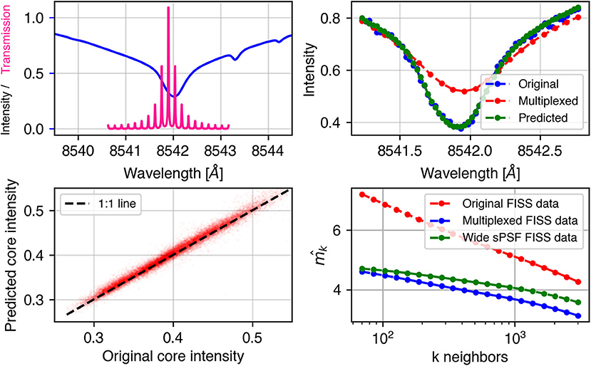
Figure 4. (Top left) The spectral transmission profile is ($\text{magenta}$ scaled by 9 for best representation) applied to the spectral profiles overlaid over the average Ca II 8,542 Å line. (Top right) Sample spectral profile from the multiplexing ($\text{red}$), the retrieved spectral profile ($\text{green}$) and the original spectral profile ($\text{blue}$); (Bottom left) Retrieved line core intensity from this approach vs the original line core intensity; (Bottom right): Maximum Likelihood Intrinsic Dimensionality Estimate for the original FISS data, the multiplexed FISS data and the data convolved with the wide sPSF in section 3.1.

We applied the transmission profile to the FISS data used in section 3.1 where we downsampled the number of spectral samples by 3 for this particular example. A sample deconvolution is presented in the top right panel of Figure 4, which shows a good agreement between the original and deconvolved spectral profiles. The bottom left of Figure 4 shows the scatter of the derived line core intensity of the multiplexed line vs. the original line core intensity. We achieve a RMS of the retrieved line core intensity of about 2% for this numerical setup. This is about three times worse than the previous experiment with FISS data in section 3.1. Our result is close to the precision obtained by Asensio Ramos (2010) where the author uses a single FP etalon with a prefilter.

To explain the lower precision of this multipeaked-multiplexing deconvolution approach compared to the deconvolution of the wide sPSF in section 3, we evaluate the dimensionality of the data. The dimensionality quantifies how much information is contained in the observations and can be used to evaluate the losses due to the spectral multiplexing. We computed the maximum likelihood intrinsic estimated dimensionality [MLIED, introduced by Levina and Bickel (2004) and suggested for spectroscopic use by Asensio Ramos et al. (2007)], which is an estimate of the dimensionality of the data based on phase density distribution. The bottom right panel of Figure 4 shows the dimensionality estimate for the original data, the multiplexed data, and the data convolved with a wide sPSF vs. the number of neighboring spectra used for the computation of the dimensionality. We find that the dimensionality of the multipeaked-multiplexed data is lower than the data convolved with a wide sPSF, while the original data has the highest dimensionality. It is expected since the convolution process introduces a loss of information. This greater loss of information is why the multipeak approach (as modeled in this section) results in a lower precision compared to the results those for a single, broad sPSF.

This approach, evaluating spectral dimensionality, could be used in future design studies of instruments as a way toward building more efficient instruments, optimizing throughput and preservation of spectral information. Further work is needed to connect the dimensionality analysis (and resulting choice of instrumental sPSF) with the accuracy and precision of the retrieval of physical information from the spectral profiles via the optimal choice of parameters for the FP system.

5. Conclusions and Future Work

We have presented a novel way to perform deconvolution of spectral data with deep learning. Our method is robust and reliable if the sPSF of the instrument is well known a priori and we have a reliable training set. Our method can deconvolve a single, 40-wavelength spectrum in 0.3 microsecond on a NVIDIA TITAN RTX GPU with a photometric precision of the line core intensity of <1%. The speed of the proposed algorithm makes it very effective for processing large numbers of spectra, with further improvements possible if the deconvolution is performed on batches of data on a GPU. With the next generation of solar instruments (such as the VTF at the DKIST), which will produce terabytes of spectral data per day, the speed of deconvolutional techniques will become increasingly important.

The technique was demonstrated here only for non-polarized spectroscopic measurements, but full spectropolarimetric measurements (including also the spectral dependence of the circularly and linearly polarized components of the signal) are a key aspect of observational solar science. There is no conceptual reason why this method could not be extended to the measurement of the Stokes profiles, given suitable training sets. However, since the polarized components of the signal tend to be just a small fraction of the overall signal (a few percent or less), any systematic errors introduced into the deconvolved profiles might bias the recovery of the information about the magnetic field. Future work will evaluate the application of this method to this common usage scenario.

We successfully recovered spectral line profiles observed with a multipeaked spectral transmission profile, as suggested before in Asensio Ramos and López Ariste (2010), using a theoretical dual Fabry-Pérot etalon instrument with optically realistic parameters. Our numerical experiments showed that a careful choice in the separation of the peaks of the transmission profile allows the retrieval of the spectral line profiles with a photometric precision of about ~2% while requiring 3 times fewer spectral samples. This could be used in the design of future Fabry-Pérot based instruments that would require fewer measurements (higher cadence) and potentially have higher transmission (shorter exposure times).

Future work will include obtaining a more suitable dataset for improving the results from the experiment with IBIS data in section 3.2. In order to apply this deconvolutional approach to real observations in a routine manner we will need training sets consisting of low and high resolution data of a variety of regions on the Sun. One approach would be to obtain nearly simultaneous observations of the same region of the Sun with low and high spectral resolution instruments at comparable spatial resolution. Another feasible way to create the training dataset is by numerically convolving data from a high-spectral-resolution instrument with the known sPSF of the low-spectral-resolution instrument to generate simulated observations Both approaches have advantages and disadvantages but provide alternative approaches to real world applications of this method. We therefore hope that future instruments will consider the approaches described here and in Asensio Ramos and López Ariste (2010) to leverage the advantages of machine learning and compressive sensing to more efficiently retrieve information from the solar spectrum and further our understanding of the Sun.

Data Availability Statement

The datasets and the code for this study can be found in the github repository of the author, https://github.com/momomolnar/SPSF_remove.

Author Contributions

KR proposed the setup of the two problems and suggested the approach to solving it and obtained the FISS data. KR and MM acquired the IBIS data at the DST. MM reduced the IBIS data and constructed the CNNs with help from CO and IM. MM performed the tests of the accuracy of the methods. All authors contributed to the manuscript.

Funding

MM was supported for the work on this article from the GEH fellowship provided from the University of Colorado, Boulder. Funding for the DKIST Ambassadors program was provided by the National Solar Observatory, a facility of the National Science Foundation, operated under Cooperative Support Agreement Number AST-1400405. CO acknowledges support from the UK's Science and Technology Facilities Council (STFC) doctoral training grant ST/R504750/1.

Conflict of Interest

The authors declare that the research was conducted in the absence of any commercial or financial relationships that could be construed as a potential conflict of interest.

Acknowledgments

MM would like to thank the organizers of the ML in Helio conference for the support to attend this great workshop. CO is grateful to the members of the National Solar Observatory for many scintillating discussions. The authors would like to thank Kyeore Lee, Jongchul Chae, and Kwangsu Ahn for generously providing the FISS spectra. Furthermore, the authors would like to thank the referees for their comments which helped improve the manuscript and Andres Asensio Ramos for the useful discussions which helped with the CNN approach and the Maximum Likelihood Dimensionality Estimate. The National Solar Observatory (NSO) is operated by the Association of Universities for Research in Astronomy, Inc. (AURA), under cooperative agreement with the NSF. IBIS has been designed and constructed by the INAF/Osservatorio Astrofisico di Arcetri with contributions from the Università di Firenze, the Università di Roma Tor Vergata, and upgraded with further contributions from NSO and Queens University Belfast.

Footnotes

1. ^For symmetric line profiles, Doppler velocity does not depend on R.

References

Abadi, M., Agarwal, A., Barham, P., Brevdo, E., Chen, Z., Citro, C., et al. (2015). TensorFlow: Large-Scale Machine Learning on Heterogeneous Systems. Available online at: tensorflow.org.

Google Scholar

Asensio Ramos, A. (2010). Compressed sensing for next generation instruments. Astron. Nachrich. 331:652. doi: 10.1002/asna.201011394

CrossRef Full Text | Google Scholar

Asensio Ramos, A., and López Ariste, A. (2010). Compressive sensing for spectroscopy and polarimetry. Astron. Astrophys. 509:A49. doi: 10.1051/0004-6361/200913019

CrossRef Full Text | Google Scholar

Asensio Ramos, A., Socas Navarro, H., Lopez Ariste, A., and Martinez Gonzalez, M. J. (2007). The intrinsic dimensionality of spectropolarimetric data. Astrophys. J. 660, 1690–1699. doi: 10.1086/513069

CrossRef Full Text | Google Scholar

Baranyi, T. (1986). Study of solar hα line profiles by means of filtergrams. Publ. Debrecen Heliophys. Observ. 6:25.

Google Scholar

Baranyi, T., and Ludmány, A. (1983). Synthesis of Hα-profiles from filter transmission functions. Publ. Debrecen Heliophys. Observ. 5, 595–602.

Google Scholar

Beckers, J. M., Dickson, L., and Joyce, R. S. (1975). Observing the sun with a fully tunable Lyot-Öhman filter. Appl. Opt. 14, 2061–2066. doi: 10.1364/AO.14.002061

PubMed Abstract | CrossRef Full Text | Google Scholar

Caccin, B., Falciani, R., Roberti, G., Sambuco, A. M., and Smaldone, L. A. (1983). Bidimensional analysis of solar active regions and flares - part one - imaging spectroscopy with universal birefringent filters. Solar Phys. 89, 323–339. doi: 10.1007/BF00217254

CrossRef Full Text | Google Scholar

Caccin, B., and Roberti, G. (1979). A method for a rough reconstruction of line profiles from a series of narrow-band filtergrams. Mem. Soc. Astron. Ital. 50, 393–404.

Google Scholar

Cauzzi, G., Reardon, K., Rutten, R. J., Tritschler, A., and Uitenbroek, H. (2009). The solar chromosphere at high resolution with IBIS. IV. Dual-line evidence of heating in chromospheric network. Astron. Astrophys. 503, 577–587. doi: 10.1051/0004-6361/200811595

CrossRef Full Text | Google Scholar

Cavallini, F. (2006). IBIS: A new post-focus instrument for solar imaging spectroscopy. Solar Phys. 236, 415–439. doi: 10.1007/s11207-006-0103-8

CrossRef Full Text | Google Scholar

Chae, J., Park, H.-M., Ahn, K., Yang, H., Park, Y.-D., Nah, J., et al. (2013). Fast imaging solar spectrograph of the 1.6 meter new solar telescope at big bear solar observatory. Solar Phys. 288, 1–22. doi: 10.1007/s11207-012-0147-x

CrossRef Full Text | Google Scholar

Goodfellow, I., Bengio, Y., and Courville, A. (2016). Deep Learning. MIT Press. Available online at: http://www.deeplearningbook.org.

Google Scholar

He, K., Zhang, X., Ren, S, and Sun, J. (2016). “Deep residual learning for image recognition,” in 2016 IEEE Conference on Computer Vision and Pattern Recognition (CVPR) (Las Vegas, NV), 770–778. doi: 10.1109/CVPR.2016.90

CrossRef Full Text | Google Scholar

Kentischer, T. J., Schmidt, W., von der Lühe, O., Sigwarth, M., Bell, A., Halbgewachs, C., et al. (2012). “The visible tunable filtergraph for the ATST,” in Proceedings Vol. 8446, Ground-based and Airborne Instrumentation for Astronomy IV of Society of Photo-Optical Instrumentation Engineers (SPIE) Conference Series, 844677 (Amsterdam).

Google Scholar

Kingma, D. P., and Ba, J. (2014). Adam: A Method for Stochastic Optimization. arXiv[Preprint]. arXiv:1412.6980. Available online at: https://arxiv.org/abs/1412.6980.

Google Scholar

Levina, E., and Bickel, P. J. (2004). “Maximum likelihood estimation of intrinsic dimension,” in Advances in Neural Information Processing Systems 17. (Vancouver, BC: MIT Press), 777–784.

Google Scholar

Reardon, K. P., and Cavallini, F. (2008). Characterization of Fabry-Perot interferometers and multi-etalon transmission profiles. The IBIS instrumental profile. Astron. Astrophys. 481, 897–912. doi: 10.1051/0004-6361:20078473

CrossRef Full Text | Google Scholar

Richardson, W. H. (1972). Bayesian-based iterative method of image restoration*. J. Opt. Soc. Am. 62, 55–59. doi: 10.1364/JOSA.62.000055

PubMed Abstract | CrossRef Full Text | Google Scholar

Tritschler, A., Rimmele, T. R., Berukoff, S., Casini, R., Kuhn, J. R., Lin, H., et al. (2016). Daniel K. Inouye Solar Telescope: high-resolution observing of the dynamic Sun. Astron. Nachrich. 337:1064. doi: 10.1002/asna.201612434

CrossRef Full Text | Google Scholar

van Noort, M., Rouppe van der Voort, L., and Löfdahl, M. G. (2005). Solar image restoration by use Of multi-frame blind de-convolution with multiple objects and phase diversity. Solar Phys. 228, 191–215. doi: 10.1007/s11207-005-5782-z

CrossRef Full Text | Google Scholar