Neural Network Based Identification of Energy Conversion Regions and Bursty Bulk Flows in Cluster Data

Introduction

As sensor resolutions and sampling frequencies increase, data available from space missions is steadily increasing. For example, the SMILE mission will generate 30 Gbits/orbit of data (Raab et al., 2016). Processing these data requires large amounts of time spent by researchers in order to identify interesting events. For example, Paschmann et al. (2018) assembled a database with thousands of manually selected events from the MMS mission.

Pattern recognition tasks can be handled very well by the human brain which has a highly complex, non-linear and parallel structure (Haykin, 2009). Such an information processing system is able to perform these tasks much faster than today's computers. An artificial neural network is based on a simplified model of the biological neural network and brings the pattern recognition power of the brain into the world of computers.

As another example, Wing et al. (2003) showed the application of a multilayer feedforward neural network in the classification of radar signals from ionospheric irregularities. The neural network implementation correctly classified 98% of the signals.

In this paper we show results obtained by using a feedforward neural network for automatically locating regions of interest in time series. We searched for events in data from the Cluster mission, consisting of four identical spacecraft launched in pairs in July and August 2000, with a perigee of 4 R_E and an apogee of 19.6 R_E (Escoubet et al., 2001). The mission, whose operational phase started in February 2001, allows for in situ exploration of particle and field data, with emphasis on investigations that require multi-point data and techniques—for example, analysis of vector fields, like deriving current density from magnetic field data, or examination of magnetospheric boundary layers, like, e.g., the magnetopause. While in the following we concentrate on Cluster data, the broader goal of the paper is to investigate and illustrate the potential benefits of applying neural networks to time series of space physics interest. We aim to provide examples of using NN algorithms to quickly identify specific events, and by doing so to enable automated build-up of event databases. This can help a better exploitation of big volumes of data, much of which are time series, and by that a better view over the phenomena under study and a better insight to the relevant physics.

In the next section we present the type of neural networks architecture used in this paper and detail the software implementation of the algorithm. In section Neural Network Identification of ECRs: Key Questions, we describe several difficulties encountered during the application of the algorithm and the solutions to overcome those. In sections Neural Network Identification of ECRs: Comparison With an Algorithmic Approach and Neural Network Identification of BBFs, we present the application of this algorithm on two types of time series data provided by instruments onboard Cluster spacecrafts, namely energy conversion regions (ECRs) and bursty bulk flows (BBFs). These two examples illustrate the cases of low and high signal to noise ratio, for ECRs and BBFs, respectively, and provide qualitative information on the impact of this parameter, as well as a test bed for an upcoming quantitative assessment. In the last section we present our conclusions.

Neural Networks

Introduction: Various NN Types

Depending on the interconnection between the artificial neurons, neural networks can have different architectures. We further present three main classes:

• Single-layer feedforward networks: contain just an input and an output layer. The information is passed from the input directly to the output. This network architecture contains only one layer of processing neurons, as the input layer does not perform any computations.

• Multi-layer feedforward networks: contain more than one processing layer. Information is passed from the input layer to the output layer via one or more hidden layers.

• Recurrent networks: these networks contain at least one feedback loop connecting the output to the input.

Neural networks can learn either helped by a “teacher” or without one. The first case is called supervised learning and it involves a previously known set of input-output pairs that can be presented to the network. When learning without a “teacher,” the method is called unsupervised learning. In this case, the network attempts to split the input data in different classes. A combination of the two methods is reinforcement learning, where the network is just presented with the consequences of its actions. In this case, the network attempts to minimize a given criterion by modifying the decisions it makes.

Feedforward Back Propagation NN

In order to identify the regions of interest in time series, we make use of a feedforward back propagation neural network, which is of single or multi-layer feedforward network type. The feed-forward direction refers to the traveling of the processed input toward the output when the trained network is used. The back propagation refers to the traveling of the error backwards through the network as part of the training of the network.

During the training phase, the network learns to map a series of input vectors to the corresponding, known, output vectors. The learning process modifies the values of the inter-neuron connection weights.

The first layer of the network, the input layer, has the size equal to the size of the input vector and does not perform any computations. Its function is to feed the input information to the network. The next layers, one or more hidden layers or directly the output layer, process the information.

As data travel through the network, it is adjusted via the inter-neuron connection weights. Based on these inputs, each neuron computes its activation function. The usual types of activation functions are sigmoid and linear, and both of them are used in this paper.

The forward mechanism involves the processing of the input data by the neurons, through use of weights and transfer functions. While the latter are fixed, the weights of the network are adjusted during the training process. Data are multiplied with the corresponding weights and the input of each neuron is computed as the sum of the weighted input values:

$\begin{array}{l}{I}_j^{(1)}={\displaystyle \sum _{i=1}^m}{\omega }_{ji}{O}_i^{(0)}\end{array}$

Where

• $I_j^{(1)}$ is the input of neuron j from layer 1

• ω_ji is the weight of the connection from input i to neuron j

• $O_i^{(0)}$ is the output of the i-th element of the previous layer (input value in the case of the first layer of neurons)

• m is the number of elements of the previous layer (input in the case of the first layer of neurons).

The computed weighted sum $I_j^{(1)}$ is further passed to the activation function of the neuron j and the corresponding output computed:

$\begin{array}{l}{O}_j^{(1)}=f(I_j^{(1)})\end{array}$

Where

• $O_j^{(1)}$ is the output of neuron j from layer 1

• f is the activation function of the neuron

In case of the last layer, the output ($O_j^{(1)}$) of the neuron is an element in the output vector of the network.

During training, the values of the corresponding output vector for a given input vector are known. The error vector (e) is computed as the difference between the desired output and the actual output:

$\begin{array}{l}e=D-O\end{array}$

Where

• D—desired output vector

• O–actual output vector.

The aim of the algorithm is to minimize the error, so the weights are adjusted backward from the output, in an iterative process:

$\begin{array}{l}{\omega }_{ji}(n+1)={\omega }_{ji}(n)+\alpha \left[\Delta {\omega }_{ji}(n-1)\right]+\eta {\delta }_j(n)I_i(n)\end{array}$

Where

• ω_ji(n + 1) is the adjusted weight (step n + 1)

• ω_ji(n) is the unadjusted weight (step n)

• α is the momentum constant

• η is the learning rate

• δ_j is the local gradient—takes into account the error and the derivative of the activation function.

Essentially, the training phase represents the non-linear optimization of the weights, by using specific functional forms for the activation functions and interconnection between neurons. The learning rate and momentum constant are fixed parameters for a given instance of the network, that can be adjusted during the training phase. Together with the number of layers and the number of neurons in each layer, they represent the global parameters of the network. The user has to tune these parameters during the training phase in order to improve the results of the network. As detailed under Section Neural Network Identification of ECRs: Key Questions, the key tasks of the training phase are both the training per se and identifying the network configuration that optimizes the results.

The training stops when one of these conditions is met:

• The error drops below a certain value

• The specified number of training epochs was reached

• The error decrease rate is slow enough.

Key Features/Parameters

The sizes of the input and output layers are determined by the sizes of the input and corresponding output, respectively. The hidden layer size is determined experimentally by the user. There is no fixed rule that specifies the size or even the presence of the hidden layer.

In general, an increase in the size of the hidden layer can help the network to better learn the features of the training set. On the other hand, if the network size is increased too much, it might lose its ability to generalize and therefore to address data sets which are different from the training set—which is the actual goal of the training. A correctly configured and trained NN must be able to accurately evaluate new data, based on key features learned from the training set.

The neural network architecture presented in this paper relies either on none or one hidden layer and can be tuned to better perform the task at hand by adjusting the size of this hidden layer, the learning rate (η) and the momentum constant (α). Further degrees of freedom that need to be handled are the intrinsic variability of the network results and setting the training stop condition—all detailed under Section Neural Network Identification of ECRs: Key Questions.

Software Implementation

We implemented a feedforward neural network algorithm (private communication by Simon Wing) in C. The C programming language gives more flexibility in choosing the platform where to run the software (Linux or Windows). For switching between platforms, the program requires only a recompilation on the target platform.

The program configuration parameters are read from a file, whose name is given at runtime as a command line parameter. Inside the parameter file, the user must specify:

• Number of layers of the network

• Transfer function for each layer

• Number of neurons for each layer

• Number of training pairs

• Name of the file containing training data (input-output pairs)

• Number of testing pairs

• Name of the file containing testing data (input data)

• Name of the file containing the evolution of the error rate

• Name of the file containing the response of the network to the testing data.

The parameters that control the evolution of the network during training, the learning rate and the momentum, are specified inside the C code and can be modified if needed. This setup gives the user the possibility to explore in parallel multiple network configurations. A simple script can start the predefined configurations, each with its separate output file. A batch system allows the execution of multiple instances in parallel, each with different parameters and input data. This allows the user to search the parameter space more efficiently.

Neural Network Identification of ECRs: Key Questions

The manual examination of the Cluster plasma sheet data from the summer of 2001 provided a first set of energy conversion regions (ECRs; Marghitu et al., 2010), where E·J ≠ 0, with E the electric field and J the current density. Estimates of E are typically available on Cluster from more than one instrument, providing a necessary redundancy when the electric field is low, while J is inferred from the magnetic field, B, measured by the four Cluster satellites, as a direct application of Ampère's law.

More specifically, the electric field, was derived as E = –V × B, with plasma velocity, V, inferred from the Hot Ion Analyzer (HIA) and Composition and Distribution Function (CODIF) sensors of the Cluster Ion Spectrometer (CIS) experiment. At each time, the electric field was obtained as an average value, by using ion data from Cluster 1, Cluster 3, and Cluster 4, where one or both sensors were operational (no CIS sensor was operational on Cluster 2). Data from the Electric Field and Wave (EFW) experiment were only used to cross-check the CIS estimates. EFW provides just the spin plane projection of the electric field and the assumption E·B = 0 is needed to derive the full electric field vector. In the tail plasma sheet, where we searched for ECR events, the angle between the magnetic field vector and the Cluster spin plane was in general too small for inferring the missing electric field component (perpendicular to the spin plane) from the condition E·B = 0. Therefore, EFW data were just used to cross-check the spin plane electric field, in particular the dawn-dusk, Ey component (Ex, typically small and affected by a Sun offset, is less reliable). The current density, J, was computed from magnetic field data of the FluxGate Magnetometer (FGM) experiment, by using the Curlometer method (Dunlop et al., 2002), taking care of the spacecraft separation, as well as planarity and elongation of the Cluster tetrahedron (see below). For further details on the electric field and current density estimates, used to derive the power density E·J, the reader is referred to Marghitu et al. (2006).

Among the observed ECRs, some were concentrated generator regions (CGRs), E·J < 0, where mechanical energy is converted into electromagnetic energy, while others, more numerous in the geomagnetic tail, were concentrated load regions (CLRs), E·J > 0, where the sense of energy conversion is reversed. As illustrated in Figure 1, in both cases energy conversion is rather well-defined and observed for a relatively short time (a few minutes to a few tens of minutes). Since energy conversion is associated with interesting signatures in the plasma parameters (notably plasma velocity and related BBFs), and is known to be an important ingredient of key plasma processes, it appeared as useful to replace the time-consuming manual search with an automated procedure.

FIGURE 1

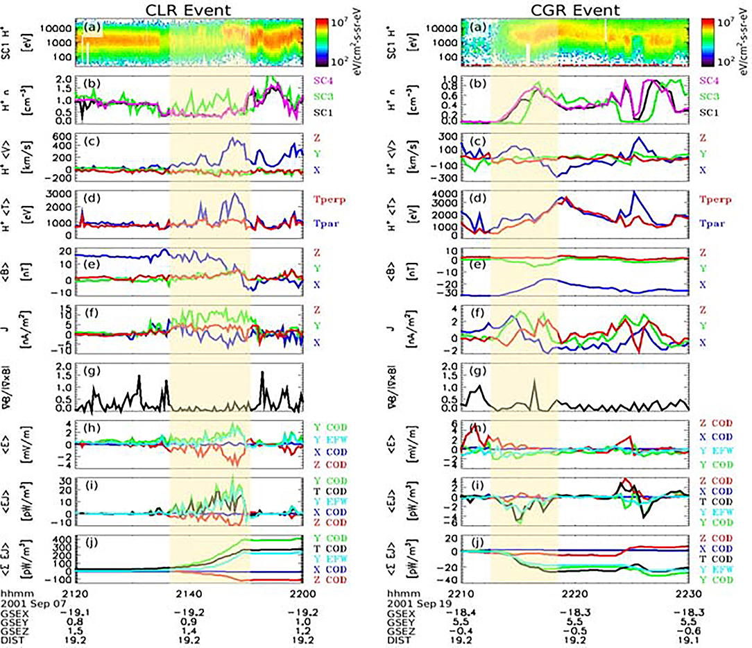
Figure 1. Left: CLR Event, Right: CGR event—after (Marghitu et al., 2010).

An algorithmic procedure has been developed by Hamrin et al. (2009a) which led to the identification of 151 ECR events, of which 116 CLRs and 35 CGRs, in the Cluster crossings of the plasma sheet from 2001. The adjusted and refined procedure was applied later on to Cluster plasma sheet crossings from 2001, 2002, and 2004 (Hamrin et al., 2010), resulting in a total of 555 ECRs, of which 428 CLRs and 127 CGRs. A broader set of events, extended to cover also 2003 and 2005 (with due care to the small Cluster tetrahedron size in 2003 and multi-scale configuration in 2005), was used to select the NN training base, consisting of 81 CLRs and the testing set consisting of 326 CLRs (see section Selection of the Training Set).

The 81 CLRs selected for training had the following distribution over 2001–2005: 11 of 2001, 28 of 2002, 19 of 2003, 21 of 2004, and 2 of 2005. The testing set consisted of 326 events, distributed as follows: 59 of 2001, 107 of 2002, 46 of 2003, 108 of 2004, and 6 of 2005. As indicated by Hamrin et al. (2009a), for all selected ECRs the tetrahedron was reasonably regular (elongation and planarity <0.4), which applied also for the events of 2003 and (few) of 2005. Moreover, ECR events that were too short (<100 s), too weak (absolute value of average E·J < 0.4 pW/m³, absolute value of integrated power density <200 pJ/m³), or too close to the kinetic regime (duration multiplied by plasma velocity <5 proton gyro-radii) were not selected. Further details of the event selection algorithm are provided by Hamrin et al. (2009a). While specific thresholds of this procedure were tuned manually, its application provided a fair selection of ECR events, whose features could be examined subsequently in a consistent manner (Hamrin et al., 2009a,b, 2010).

In a first stage, the trained NNs were used to identify both CLRs and CGRs. Accordingly, the NN output was a vector of the same size as the input data, populated with one of three values: 1 for CLRs, −1 for CGRs, and 0 in rest. Later on, as described below (sections Sliding Window Approach, Selection of the Training Set), we concentrated just on CLRs.

Size of the Input/Output Layer

Our first approach to identify energy conversion events with neural networks consisted of dividing the data into fixed size intervals (of about 100 elements). For each input interval, we had a corresponding output interval of the same size. This approach resulted in a highly complex network architecture, with 100 input neurons, a hidden layer of various sizes, and 100 output neurons. Since the feed-forward backpropagation NN we used was fully connected (every neuron in a layer was connected to all the neurons in the next layer), the training algorithm had to compute a large number of weights, which required significant training time and computer resources (memory, cpu). The trained network was also not very good in identifying the events. The data used to train the network consisted of concatenated intervals of satellite readings, containing both event (1 or −1 desired output) and non-event data (0 desired output), of which non-event data were by far dominant, therefore the trained network regarded the non-event data as the “right” ones and mostly ignored the event data.

Use of Synthetic Data for Training and Testing

Using real E·J data raised additional problems: the training set was limited and the data used for training could not be explored later—in a consistent manner—for the presence of CLRs and CGRs. In order to overcome these problems, we tried to use synthetic data for training and testing the NN. When building the synthetic data sets, we randomized the intensity, duration, and sign. During the tests with synthetic data, we noticed an improvement in detection for less complex network configurations. The network worked better for a smaller number of neurons on the hidden layer, but after training with more input data.

For simplicity, we further considered only the search for CLR events (E·J > 0), as presented in section Selection of the Training Set. This search is also similar to the case of BBFs (section Neural Network Identification of BBFs), where events are as well-positive and NN output is accordingly just 1 (event) and 0 (non-event). Moreover, in the tail plasma sheet CLRs dominate over CGRs, consistent with the large-scale load character of this region.

Sliding Window Approach

In order to decrease the training time and the complexity of the network, we opted eventually for another structure of the NN by implementing a sliding window algorithm. The sliding window consists of a certain number of input neurons, typically more than one, and just one output neuron; which implies a great decrease in the complexity of the NN and accordingly of the training time (from days to tens of minutes). As the window moves across the time series, the output is 1 when the window slides over the CLR event.

Selection of the Training Set

During the tests with real and synthetic data we noticed the importance of a heterogeneous and representative selection of input data for training the network. By including many non-event data points (associated with an output value of 0), the network is biased toward false negatives (more values of 0 in the output), therefore a balanced input selection is required (see also Section Size of the Input/Output Layer).

Starting from the dataset of ECRs observed in 2001, 2002, and 2004, analyzed by Hamrin et al. (2010), extended to cover also 2003 and 2005 (as described above), we constructed training sets with equally distributed events, in duration or intensity. In the data presented to the network during training, one must maintain a balance between event and non-event intervals. Given that the quality of the network training is judged by the mean error of the output (difference between desired and actual output), if one uses mostly non-event intervals (i.e., mostly 0 desired output) a network trained to supply mostly 0 will be wrongly considered well-trained. By using a better tuned training set, we managed to improve the detection accuracy of the NN.

A key question for this better tuning was the uniform selection of training data. For this aim, we sorted the events considering their duration, as well as their intensity, quantified by the median E·J value (similar to Hamrin et al., 2009a). The median was computed over the length of each event, consisting of at least 25 points (minimum duration 100 s, with 4 s per point—see also the brief description of the event selection algorithm above). After sorting the events, we tested two selection methods: a linear sampling, 1 out of n, and a logarithmic sampling, to take into account that most events are weak, i.e., of short duration and low intensity While the linear sampling selects mostly weak events, and thus is essentially biased comparable to the case of dominant non-event intervals, the logarithmic sampling emphasizes longer/stronger events, which turns out to compensate this bias and to provide better results. Hamrin et al. (2009a) found that intensity is indeed distributed close to logarithmic, while Hamrin et al. (2009b) found the same for duration, in particular of CLRs, therefore logarithmic sampling appears to be a better choice.

While the linear selection 1 out of n is self-explanatory (every nth event), in the case of logarithmic sampling we used the natural logarithms of the respective values and made the selection according to the following formula:

$\begin{array}{l}Index=1+(N-1)·\frac{ln\left(\frac{y_1+j\frac{y_N-y_1}{M}}{y_1}\right)}{ln\left(\frac{y_N}{y_1}\right)}\end{array}$

Where

• Index is the index of the element to be selected from the input set, comprising in our case 407 CLR events.

• y_{1, N} are the elements of the input set (of size N, in our case 407), from which we select elements of the training set; y₁ is the first element of the input set and y_N the last one.

• j is the index in the destination (selected) training set, containing selected elements, and runs from 0 to M; in our case M is 80 and the training set comprises 81 events.

In Figure 2 we present the duration of the events in the training set, selected by linear sampling 1 out of 5 (top panel-red line) and logarithmic sampling (top panel-blue line), as well as the duration of the events used for testing (bottom panel). The full set of events includes 407 CLRs, the training sets 81 events, and the testing set 326 events. For logarithmic sampling, 81 was the maximum number that ensured distinct indices after rounding at the low index end. For the linear selection, 1 out of 5 provides a training set of similar size with the logarithmic selection. As expected, the logarithmic sampling provides a more uniform selection as compared to the linear sampling, that a is, a somewhat better representation of the longer events. The plots are similar (not shown) when duration is replaced by intensity, in agreement with the distributions observed by Cluster (Hamrin et al., 2009a,b).

FIGURE 2

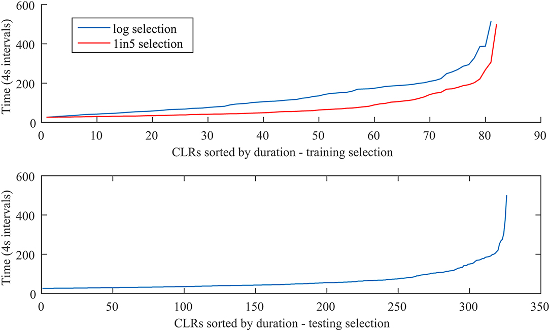
Figure 2. CLRs sorted by duration—training selection (top), testing selection (bottom). The top panel shows both the logarithmic selection (blue) of 81 events and the linear selection (red) 1 out 5, which provides a similar number of events with the logarithmic one. The x axis shows the event index in the respective set, while the y axis shows the event duration in Cluster spin periods of 4 s (the number on y axis should be multiplied by four to get the duration in seconds). See text for details.

Other Parameters: Momentum Constant, Learning Rate, Stop Condition, Initial Conditions

One difficulty encountered in the tests with ECR data was the unstable NN behavior, with fast growth of the weights (defining the connections between neurons) and error (i.e., the difference between the actual response of the NN and the target response) sometimes leading to numerical overflow.

The momentum constant (α) controls the adjustment of the network's weights, based on the previous evolution of the weight. The value of α must be kept >-1 and smaller than 1. A value of 0 means no momentum influence during training the network. The momentum constant can prevent the network from stopping in a local minimum during training. In our tests, we found that a momentum constant of 0.5 favors the stability of the network.

A smaller learning rate parameter (η) determines a smaller change in the synaptic weights of the network from one iteration to another. If the learning rate parameter is too large, in order to speed up the training, the resulting large changes of the weights may render the evolution of the network unstable during the training phase. The value of the learning rate parameter should be kept above 0 and less or equal to 1. In practice, we found appropriate a small η value, of 0.0001.

Two more important features proved to be the stop condition and the intrinsic variability of the network. Thus, the stop condition had to be formulated in terms of relative decrease in the error, as opposed to a fixed number of iterations. The intrinsic variability of the network was related to the randomly selected initial weights. In practice, the network was trained several times, and the best instance selected for further operation.

Neural Network Identification of ECRs: Comparison With an Algorithmic Approach

The detailed examination of the results on real E·J data (not concatenated individual events) shows that the NN identifies neighboring events as separate ones, while the semi-automatic algorithmic procedure set up by Hamrin et al. (2009a) includes a post-processing that merges such neighboring events into a single one. As detailed below, since post-processing introduces further degrees of freedom, we decided to skip it for the time being and to compare the results in a way that is less sensitive to this step, by using the cumulative sum of E·J.

In Figure 3 we present a sample output of the NN search for ECR events over a time interval of ~3 h. The NN configuration in this case included no hidden layer and the sliding window (Section Sliding Window Approach) had five points. During our tests, we explored the use of different window sizes, from 5 to 101 points, with various hidden layer sizes, from 0 (no hidden layer) to 71. Following the evaluation detailed below, the NN configuration behind Figure 3 provided the results that we regarded as the best match to the algorithmic approach, used for reference. This means that most events identified by the algorithmic approach were also detected by the NN (which does not exclude additional events detected by the NN).

FIGURE 3

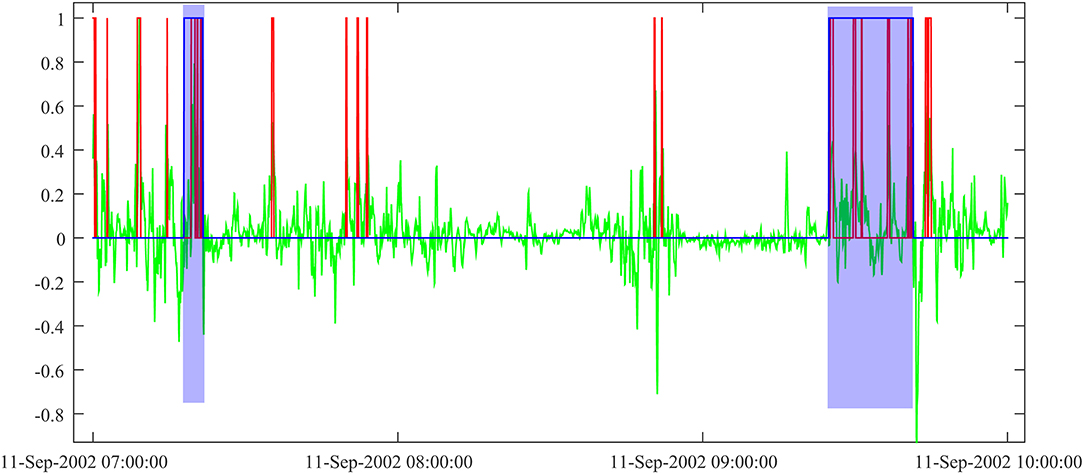
Figure 3. NN output on E·J data: NN output (rounded) in red, E·J in green (normalized to the maximum value of the time interval, here 17.4 pW/m³). Events found by the algorithmic approach are shaded in blue.

In order to evaluate the multiple network configurations, we compared the NN output with the results of the algorithmic approach by building pie charts and scatter plots for all network configurations, as illustrated in Figure 4. This allowed a quick and overall visual comparison of the events selected by the NN with those selected by the algorithmic approach. Figure 4 corresponds to a NN with no hidden layer and an input sliding window of five elements. The events used for training were logarithmically distributed in duration and selected from Cluster data between 30th May 2001 and 30th December 2004.

FIGURE 4

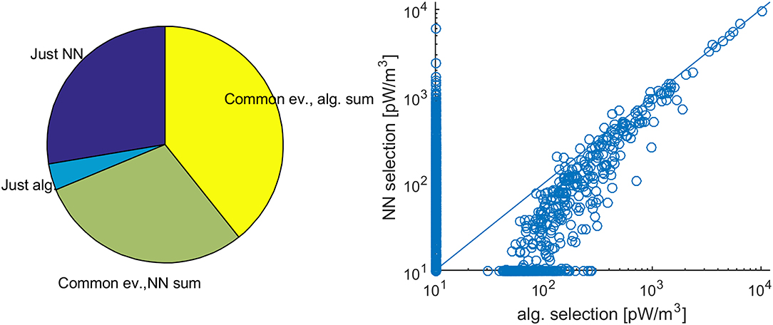
Figure 4. Comparison between the algorithmic approach and NN output. Pie chart representation of the total cumulative sum of E·J (left) and scatter plot of the cumulative sum of E·J for individual events, as derived by the two procedures (right). The unit for the cumulative sum of E·J is pW/m³. The scatter plot is presented on logarithmic scale, in order to emphasize the more numerous weak events (compare with Figure 2). The points on the x and y axis are identified just by the algorithmic and NN approach, respectively, and the actual cumulative sums are 0. In order to make these points visible in logarithmic representation, the value of 0 was changed artificially to 10. See text for details.

The left plot of Figure 4 shows the cumulative sum of E·J over the selected events. As hinted at above, we picked the integrated magnitude of the events since this is less sensitive to the exact definition of an event—whether the individual spikes identified by the NN are merged together, as in the algorithmic approach, or not. We also selected the pie chart for the visual representation, even if in this case the whole pie does not have the usual meaning, namely it is not equal to the sum of the slices. Nevertheless, it provides a useful tool to quickly assess the matching of the two procedures. More exactly, dark/light blue indicates events found only by the neural network/algorithmic approach, while light green/yellow shows the cumulative sum for the common events, computed over the results of the neural network/algorithmic approach. For the first, the small light blue and large dark blue slices show that the NN events is essentially a super-set of the events derived by the algorithmic approach, which looks promising. For the latter, the positive difference between yellow and light green is consistent with the visual impression of Figure 3, that the “elementary” events identified by the NN do not fully fill the merged events obtained by the algorithmic approach after post-processing.

A complementary view is provided by the scatter plot on the right side of Figure 4, which helps to substantiate further the comparison of the results by an event-oriented perspective. Each event is indicated by an empty bullet, with the cumulative sum of E·J as derived by the algorithmic/NN approach on the x/y axis. Most bullets indicate values of < ~1,000 pW/m³, consistent with the point made before that most events are observed to be short and weak (Figure 2). Most of the bullets identified by both the algorithmic and the NN approach are also slightly under the first bisector, consistent with the larger yellow slice compared to the light green one, and the respective cumulative sums of the algorithmic approach are larger than 50 pW/m³, as required by the threshold of 200 pJ/m³, indicated in Section Neural Network Identification of ECRs: Key Questions (which, when expressed in terms of cumulative sum, should be divided by the 4 s duration of each sample). Several bullets are aligned along the x and y axes, consistent with the light blue and dark blue slices of the pie chart, respectively, in the left plot of Figure 4. For these latter bullets, 10 pW/m³ were artificially added, to make them visible in logarithmic representation—whose origin here is the point (10, 10) pW/m³.

Since typical magnitudes of E and J are in the range of a few up to several mV/m and nA/m², respectively, the power density unit for E·J, and for the cumulative sum of E·J in Figure 4, is pW/m³. Note that by scaling E·J with 4 s (the duration of the sampling interval), one can derive the energy density profile along Cluster crossing of the CLR, in pJ/m³. From this perspective, by scaling the cumulative sum of E·J with 4 s and by dividing the result through the number of points (i.e., 4 s intervals), one can derive a proxy for the average energy density of each CLR event. While Cluster data provide some information on the size and lifetime of the CLR events (Hamrin et al., 2009b), the precise relevance of this proxy depends on the particular geometry of the Cluster crossing with respect to the CLR. For this reason, we prefer to show the cumulative sum of E·J and refrain from scaling this result.

The visual information provided by the pie chart and scatter plot can aid in quickly assessing the performance of the NN and is preferred here against the standard evaluation in terms of false positive and false negative events. As described above (section Neural Network Identification of ECRs: Key Questions), the definition of the “event” in the algorithmic approach—which provides our comparison benchmark—is to some extent empirical, and cannot be regarded as an “absolute” reference. The identification of the events allows for jitter in the start and end time, the NN approach can select individual smaller events corresponding to a larger, singular event of the algorithmic approach, and several new events are detected by the NN (the dark blue slice of the pie chart and the points on the y axis of the scatter plot in Figure 4). Therefore, comparing the results in terms of “events” is not straight forward and, in this case, performance assessment by means of the more flexible cumulative sum looks better suited than the classical manner.

Neural Network Identification of BBFs

Using the software developed to search for ECRs, we considered testing the functionality of the selection tool provided by the neural network implementation on other time series. We decided to explore the possibility of using this setup to locate Bursty Bulk Flow (BBF; Angelopoulos et al., 1992) events in ion velocity observed by the HIA instrument (Rème et al., 2001) on Cluster. In qualitative terms, BBFs are better defined than ECRs, meaning less weak events and a better signal-to-noise ratio. Intuitively, one can expect that an automatic pattern recognition tool will work better with BBFs. Unlike for ECRs, in the case of BBFs we did not benefit from an event database at hand, to provide the training set. On the other hand, the definition of BBF events is documented in several studies (even though there is some variability in the relevant criteria), therefore assembling a training set is significantly easier compared to ECRs. Moreover, observation of BBFs requires just single-s/c ion data, compared to multi-s/c, multi-instrument data for ECRs. This has a positive effect on the errors and on the signal-to-noise ratio.

In order to assemble the training set, we manually selected 39 events, with duration between 500 and 3,000 s and a velocity threshold of 400 km/s. The actual training set was built by extending the selection around the events to include also non-event data points and by finally concatenating the data. Similar to the ECR case, we tested several network configurations with this training set and eventually selected once again the one used with ECRs (window size 5, no hidden layer).

Figure 5 shows a representative sample output of the trained network over a ~5 h Cluster crossing of the plasma sheet. Compared to the ECR sample in Figure 3, covering a shorter interval, the NN output is less abundant (fewer red events per unit time), which is a consequence of the better signal-to-noise ratio. The event selection seems reasonably accurate, but it still requires further post-processing (i.e., joining short, neighboring events; rejecting events below the velocity threshold). For this particular time interval, the actual number of BBF events is 4 (shaded in blue), while the NN output is ~20 (counting the red rectangles/spikes). This suggests a rough multiplication factor of five, between the actual number of events and the network result. Implementing the post-processing will also make possible a quantitative assessment of the NN performance, in the standard terms of false positive and false negative events.

FIGURE 5

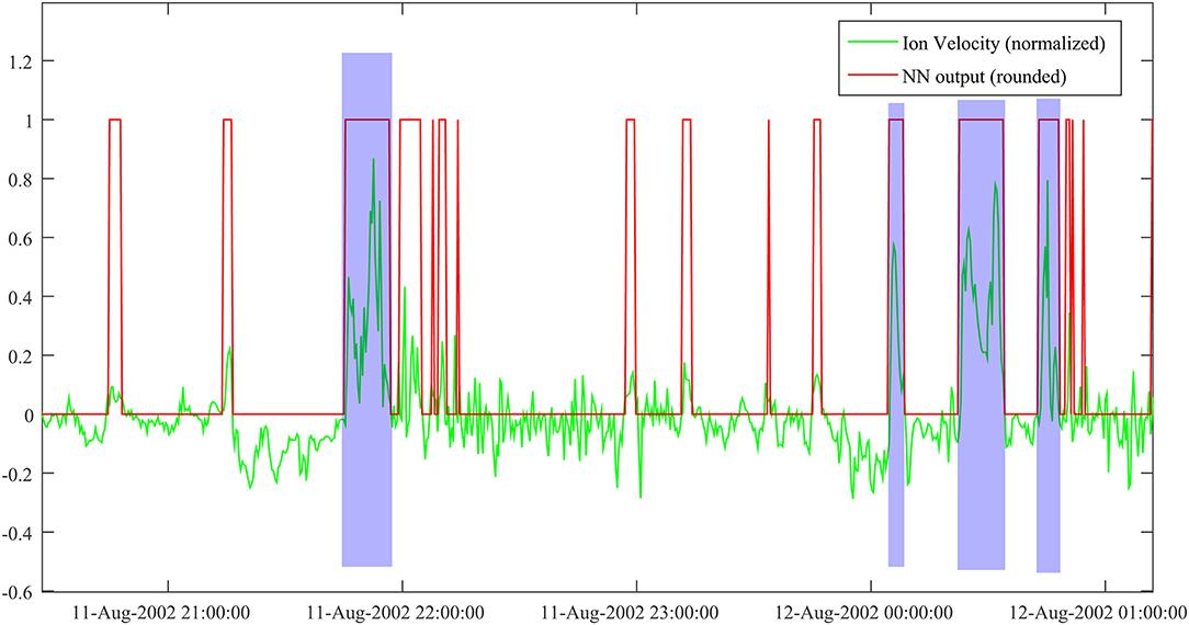
Figure 5. NN output for ion velocity data. Velocity is normalized to a maximum value of 1,000 km/s. Actual BBF events are shaded in blue.

The test data was built by using Cluster plasma sheet measurements from the tail seasons of 2001–2004, 1st of August to 10th of October. The actual tail seasons were actually somewhat longer, but we made a conservative choice, to avoid contamination with magnetosheath data on the dawn flank (before 1st of August) and on the dusk flank (after 10th of October). A preliminary count provided about 4,150 NN events, namely some 800 actual events for the rough multiplication factor of five estimated above. Compared to the training set of 39 events, the gain in the number of events is of the order of 20, which consolidates the case for using NNs in exploring time series. Obviously, in a particular case like this, the human effort to build up a large event data base, appropriate, e.g., for statistical studies, is tremendously decreased.

Conclusions

The NN approach explored in this paper provides an efficient tool to automatically identify specific events in time series. When using supervised learning, as illustrated here, a key stage is building a representative training set, to be extended by the network later on, during its nominal use. Another essential feature is that the user must explore different network configurations, by training and testing, in order to find the right setup for the problem at hand.

The effort spent on finding the proper NN setup can be considerable, as illustrated with the case of the weaker/noisier ECRs, which are also harder to identify. In such cases, the benefits of using the NN approach may appear questionable. On the other hand, for the stronger/clearer BBF events, detection is both easier and more reliable. Opposite to ECRs, the benefits of using NNs to build up large event data bases are in such cases obvious. In the future, we plan to further explore and try to quantify the connection between the noise level and the results of neural networks approaches.

Time series data are generously supplied nowadays by a broad spectrum of high-resolution satellite (and ground) experiments. Searching such data for specific events, as well as assembling relevant statistical sets, are notoriously time-consuming in space physics research. By taking advantage of machine learning tools, like neural networks, to automate such operations, the time share for creative (and rewarding) research will increase, to the benefit of both event-oriented and statistical studies.

Data Availability Statement

Publicly available datasets were analyzed in this study. This data can be found here: https://csa.esac.esa.int/csa-web/.

Author Contributions

VC implemented the C code and batch scripts and ran tests with different network configurations. OM guided the exploration of E·J and ion velocity data, helped in manually selecting the BBF training events, and evaluated the results of different network configurations. All authors contributed to the article and approved the submitted version.

Funding

This work was supported by the PRODEX project MAGICS, ESA contract 4000127660, and by the Core Program LAPLAS VI of the Romanian Ministry of Education and Research. Earlier relevant work was performed under the PECS project ECSTRA, ESA contract 4200098048.

Conflict of Interest

The authors declare that the research was conducted in the absence of any commercial or financial relationships that could be construed as a potential conflict of interest.

Acknowledgments

Helpful suggestions by Simon Wing, on optimizing the NN performance, are gratefully acknowledged. Useful discussions with Maria Hamrin and Patrik Norqvist, on the Cluster ECR database, are thankfully acknowledged too.

References

Angelopoulos, V., Baumjohann, W., Kennel, C. F., Coroniti, F. V., Kivelson, M. G., Pellat, R., et al. (1992). Bursty bulk flows in the inner central plasma sheet. J. Geophys. Res. Space Phys. 97, 4027–4039. doi: 10.1029/91JA02701

CrossRef Full Text | Google Scholar

Dunlop, M., Balogh, A., Glassmeier, K.-H., and Robert, P. (2002). Four-point cluster application of magnetic field analysis tools: the curlometer. J. Geophys. Res. 107:1384. doi: 10.1029/2001JA005088

CrossRef Full Text | Google Scholar

Escoubet, C. P., Fehringer, M., and Goldstein, M. (2001). The Cluster mission. Ann. Geophys. 19, 1197–1200. doi: 10.5194/angeo-19-1197-2001

CrossRef Full Text | Google Scholar

Hamrin, M., Norqvist, P., Marghitu, O., Buchert, S., Klecker, B., Kistler, L. M., et al. (2009a). Occurrence and location of concentrated load and generator regions observed by Cluster in the plasma sheet. Ann. Geophys. 27, 4131–4146. doi: 10.5194/angeo-27-4131-2009

CrossRef Full Text | Google Scholar

Hamrin, M., Norqvist, P., Marghitu, O., Buchert, S., Klecker, B., Kistler, L. M., et al. (2010). Geomagnetic activity effects on plasma sheet energy conversion. Ann. Geophys. 28, 1813–1825. doi: 10.5194/angeo-28-1813-2010

CrossRef Full Text | Google Scholar

Hamrin, M., Norqvist, P., Marghitu, O., Vaivads, A., Klecker, B., Kistler, L. M., et al. (2009b). Scale size and life time of energy conversion regions observed by cluster in the plasma sheet. Ann. Geophys. 27, 4147–4155. doi: 10.5194/angeo-27-4147-2009

CrossRef Full Text | Google Scholar

Haykin, S. S. (2009). Neural Networks and Learning Machines. Upper Saddle River, NJ: Pearson Prentice Hall.

PubMed Abstract | Google Scholar

Marghitu, O., Hamrin, M., Klecker, B., and Rönnmark, K. (2010). “Cluster observations of energy conversion regions in the plasma sheet,” in The Cluster Active Archive: Studying the Earth's Space Plasma Environment, eds H. Laakso, M. Taylor, and C. P. Escoubet (Dordrecht: Springer), 453–459. doi: 10.1007/978-90-481-3499-1_32

CrossRef Full Text | Google Scholar

Marghitu, O., Hamrin, M., Klecker, B., Vaivads, A., McFadden, J., Buchert, S., et al. (2006). Experimental investigation of auroral generator regions with conjugate Cluster and FAST data. Ann. Geophys. 24, 619–635. doi: 10.5194/angeo-24-619-2006

CrossRef Full Text | Google Scholar

Paschmann, G., Haaland, S. E., Phan, T. D., Sonnerup, B. U. Ö., Burch, J. L., Torbert, R. B., et al. (2018). Large-scale survey of the structure of the dayside magnetopause by MMS. J. Geophys. Res. Space Phys. 123, 2018–2033. doi: 10.1002/2017ja025121

CrossRef Full Text | Google Scholar

Raab, W., Branduardi-Raymont, G., Wang, C., Dai, L., Donovan, E., Enno, G., et al. (2016). “SMILE: a joint ESA/CAS mission to investigate the interaction between the solar wind and Earth's magnetosphere,” in Space Telescopes and Instrumentation 2016: Ultraviolet to Gamma Ray, Vol. 9905 (Edinburgh: International Society for Optics and Photonics).

Google Scholar

Rème, H., Aoustin, C., Bosqued, J. M., Dandouras, I., Lavraud, B., Sauvaud, J. A., et al. (2001). First multispacecraft ion measurements in and near the earth's magnetosphere with the identical Cluster ion spectrometry (CIS) experiment. Ann. Geophys. 19, 1303–1354. doi: 10.5194/angeo-19-1303-2001

CrossRef Full Text | Google Scholar

Wing, S., Greenwald, R. A., Meng, C.-I., Sigillito, V. G., and Hutton, L. V. (2003). Neural networks for automated classification of ionospheric irregularities in HF radar backscattered signals. Radio Sci. 38, 2-1–2-8. doi: 10.1029/2003RS002869

CrossRef Full Text | Google Scholar