Some Similarities and Differences Between the Observed Alfvénic Fluctuations in the Fast Solar Wind and Navier–Stokes Turbulence

Borovsky, Joseph E.; Mina, Tiziano

doi:10.3389/fspas.2020.00053

ORIGINAL RESEARCH article

Front. Astron. Space Sci., 31 August 2020
Sec. Space Physics
Volume 7 - 2020 | https://doi.org/10.3389/fspas.2020.00053

Some Similarities and Differences Between the Observed Alfvénic Fluctuations in the Fast Solar Wind and Navier–Stokes Turbulence

Joseph E. Borovsky¹^*

Tiziano Mina^2,3

¹Center for Space Plasma Physics, Space Science Institute, Boulder, CO, United States
²Facoltà di Matematica, Università Degli Studi di Torino, Turin, Italy
³Los Alamos National Laboratory, Theoretical Division, Los Alamos, NM, United States

Using two long data sets analyzed on equal footing, the properties of Alfvénic fluctuations in the fast (coronal-hole-origin) solar wind and Navier–Stokes turbulence are compared. A 26.4-s-long interval of hot-wire measurements in the ONERA wind tunnel is used, and a 71-h-long interval of unperturbed coronal-hole plasma measured by the WIND spacecraft at 1 AU is used. Similarities and differences between a Navier–Stokes fluid and the collisionless magnetized solar-wind plasma are discussed, as are differences between the physical natures of the advecting evolving turbulent fluctuations and the propagating non-evolving Alfvénic fluctuations. The details of the power spectral densities of the turbulence and the Alfvénic fluctuations are compared. Statistics of first and second time derivatives are examined for the wind-tunnel and solar-wind time series, and the statistics are compared with the statistics of time derivatives of phase-randomized time series. Using running medians, the statistics of flat spots in the time series of Alfvénic fluctuations is examined, which is evidence of a cellular structure to the magnetic field and velocity field. A call for a campaign of expanded coordinated future work is made.

Introduction

A side-by-side comparison is made between Navier–Stokes turbulence measured in a wind tunnel and Alfvénic fluctuations measured in the fast solar wind. Measurements of the Alfvénic fluctuations in the fast solar wind are often considered to be measurements of magnetohydrodynamics (MHD) turbulence (Tu et al., 1989; Marsch and Tu, 1990a; Bavassano and Bruno, 1992; Wicks et al., 2013; Telloni et al., 2019), although the Alfvénic fluctuations have some properties different from a turbulence. Navier–Stokes fluid turbulence comprised rapidly evolving advecting structures (eddies) that strongly interact with each other, whereas the Alfvénic fluctuations in the solar wind propagate en masse through the plasma away from the Sun and are largely non-evolving.

In the theory of MHD turbulence, Alfvénic fluctuations can only be involved in turbulence if there are counterpropagating fluctuations in order to enable non-linear interactions (Kraichnan, 1965; Dobrowolny et al., 1980). If there is turbulence acting in the fast solar wind, it is related to the inward (toward the Sun) propagating Alfvénic fluctuations, which, if they exist, are in the noise of the measurements (Wang et al., 2018). Relatedly, in the reference frame that moves outward away from the Sun at the velocity of the Alfvénic fluctuations, the plasma flow velocity component locally perpendicular to B is in the noise of the measurement, indicating little or no evolution of the magnetic structure as it propagates outward (Borovsky J. E., 2020a).

This study will make a systematic comparison of the properties of Alfvénic solar wind fluctuations with true Navier–Stokes Kolmogorov active turbulence, asking what is similar, what is different, and for the properties that are similar asking why they are similar. As will be pointed out, the Navier–Stokes Kolmogorov turbulence measurements in the wind tunnel and the MHD Alfvénic structure propagation measurements in the fast solar wind are observations of two completely different processes. Similarities might point to some universal properties.

For a sample of Navier–Stokes turbulence, hot-wire 4 × 10⁻⁵-s resolution measurements of the streamwise velocity v from the return-flow channel of the ONERA S1 wind tunnel at Modane are used (cf. Kahalerras et al., 1998; Malecot et al., 2000; Gagne et al., 2004; Podesta et al., 2009). The measurements are taken at the axis of the 24-m-diameter return channel. No grid is used in the return channel to generate turbulence; rather, as is the case for pipe flow (cf. Schlichting, 1979), the turbulence is driven by a velocity shear across a boundary layer between the wind flow and the wall (Kim et al., 1971). Some of the properties of this Navier–Stokes–turbulence time series are collected into Table 1. Applying the Reynolds-number scaling R ~ (L_eddy/L_Kolmog)^4/3 (e.g., Equation 7.18 of Frisch, 1995), where L_eddy is the large eddy size (taken to be the low-frequency breakpoint of the power spectral density), and L_Kolmog is the Kolmogorov scale (taken to be the high-frequency breakpoint of the power spectral density), with the values L_eddy = 20 m and L_Kolmog = 1.6 cm in Table 1, the large-eddy Reynolds number R for the wind-tunnel turbulence is estimated as R ~ 1.3 × 10⁴. Gagne et al. (2004) estimate the Taylor microscale to be λ ≈ 2.8 cm and the Taylor-scale Reynolds number to be R_λ ≈ 2,260.

TABLE 1

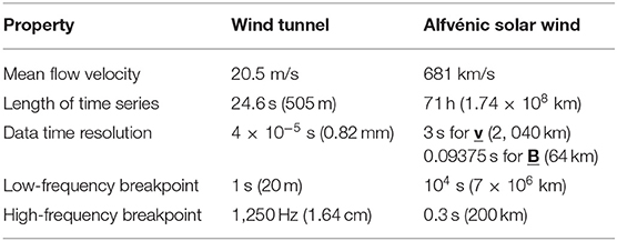
Table 1. Some properties of the wind-tunnel and Alfvénic solar-wind time series analyzed in this study.

For a sample of Alfvénic fluctuations in the fast solar wind, a 71-h interval of unperturbed coronal-hole-origin plasmas measured by the WIND spacecraft at 1 AU is used. The long sample (13:00 UT on November 4, 2005, to 12:00 UT on November 7, 2005) of data analyzed is from “Flattop 15” in Table 1 of Borovsky (2016). In Figure 1, the radial (from the Sun) flow velocity –v_x of the solar wind is plotted as a function of time for the solar-wind high-speed stream that contains Flattop 15. The flat top of the –v_x plot indicates an interval of unperturbed fast wind, unperturbed in the sense that it has not been compressed or rarefacted by interaction with slower-wind streams. The WIND spacecraft measured the plasma flow vector v with 3-s time resolution using the 3DP (three-dimensional plasma) instrument (Lin et al., 1995) and measured the magnetic-field vector B with 0.09375-s time resolution using the MFI (magnetic field instrument) (Lepping et al., 1995). Note that the 3DP velocity measurements are noisier than the MFI magnetic-field measurements, and so some of the analyses will focus on B instead of v. WIND spacecraft data are supplied in the GSE (geocentric solar ecliptic) XYZ right-hand coordinate system, where the direction X points from the Earth to the Sun, Y points from the Earth duskward in the ecliptic plane, and Z is normal to the ecliptic plane. During the 71-h interval denoted as Flattop 15 in Figure 1, the mean values ± standard deviations for some solar-wind parameters are radial flow speed –v_x = 681 ± 32 km/s, plasma number density n = 1.47 ± 0.26 cm⁻³, magnetic-field strength B_mag = 4.47 ± 0.60 nT, Alfvén speed v_A = 81.1 ± 10.5 km/s, Alfvén Mach number M_A = –v_x/v_A = 8.6 ± 2.1, ion-inertial length c/ω_pi = 190 ± 18 km, and thermal proton gyroradius r_gi = 107 ± 27 km. To estimate an effective large-eddy Reynolds number, the Reynolds-number scaling R_eff ~ (L_eddy/L_Kolmog)^4/3 is applied, where the scale size associated with the high-frequency breakpoint is used for L_Kolmog, even though it is not a Kolmogorov scale where viscosity balances the cascade rate; with the values L_eddy = 7 × 10⁶ km and L_Kolmog = 200 km in Table 1, the effective Reynolds number R for the Alfvénic fluctuations is estimated as R_eff ~ 1.1 × 10⁶. At 681 km/s, the transit time of the solar wind (= age of the solar-wind plasma) from the Sun to 1 AU is ~61 h, which is less than the 71-h duration of the interval; hence (like a wind tunnel), the beginning of the Flattop-15 plasma interval was being measured at 1 AU before the final part of the interval was created at the Sun. This 61-h transit time is also approximately the age of the plasma τ_age when it is measured at 1 AU. A large spatial scale for this interval of coronal-hole-origin solar wind is defined by causality and the age of the plasma: the spatial scale L_caus = v_Aτ_age, which is the distance an Alfvénic signal can propagate along the mean field and so represents the “domains of communication” scale size in the plasma. This value is L = v_Aτ_age = M $_{A}^{- 1}$ d, where d = 1 AU = 1.5 × 10⁸ km is the distance from the Sun to the WIND spacecraft. It would be associated with a spacecraft timescale t_caus = M $_{A}^{- 1} τ_{age}$ = 7.1 h. Another large spatial scale in this plasma is the ~5-h domains of Alfvénicity shown in Figure 14 of Borovsky (2016); it has been suggested that these domains could be associated with the large-scale open-flux-funnel structure of coronal holes. Some properties of this Alfvénic-fluctuation time series are collected into Table 1.

FIGURE 1

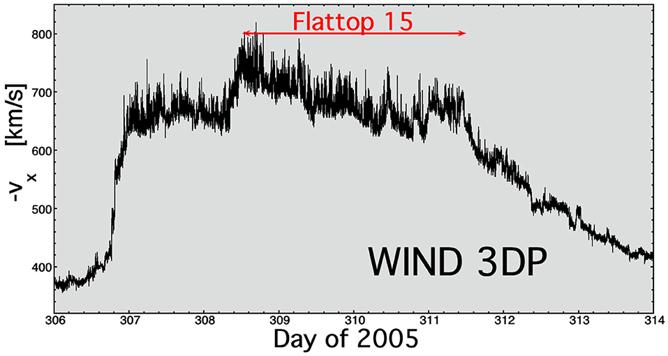
Figure 1. The high-speed stream in November 2005 that contains Flattop 15. The radial-velocity measurements were taken by the WIND spacecraft at 1 AU.

In making the comparison between the Navier–Stokes wind-tunnel measurements and the solar-wind fluctuation measurements, it would be useful to normalize the two data sets to each other, perhaps by scaling the amplitudes and the times. Owing to uncertainties, such a normalization is not made for the present study. One-time scaling could be based on the correlation time of each time series; however, the correlation time is ambiguous, and depends on the length of the time series used for its calculation. A less-ambiguous time normalization could be based on the timescale of the high-frequency Fourier breakpoint of the power spectral density of each time series. The analysis of the two time series in Similarities and Differences in the Statistics of Derivatives will be based on the timescale difference from the high-frequency breakpoint of the two series.

This article is organized as follows. In Similarities and Differences in the Medium, similarities and differences between a Navier–Stokes fluid and the magnetized collisionless solar-wind plasma are discussed. In Similarities and Differences in the Fluctuations, similarities and differences in the physical nature of the fluctuations in Navier–Stokes turbulence vs. the Alfvénic solar wind are discussed. Similarities and Differences in the Fourier Spectra examines the similarities and differences in the power spectral densities of the wind-tunnel Navier–Stokes turbulence vs. the Alfvénic fluctuations in the fast solar wind. Similarities and Differences in the Statistics of Derivatives examines the statistics of time derivatives in the wind-tunnel Navier–Stokes turbulence measurements vs. the measurements of the Alfvénic fluctuations of the solar wind. Level Shifts and Calm Regions examines flat spots in the measurement time series of the wind tunnel vs. the Alfvénic solar wind. Summary and Discussion contains a summary of findings and a discussion about the possible origin of the properties of the Alfvénic fluctuations. Similarities and Differences in the Medium also contains a summary. A call for coordinated future work is also made in Summary and Discussion.

Similarities and Differences in the Medium

A Navier–Stokes fluid (such as air) is an isotropic medium that obeys the Navier–Stokes equation for momentum transport

\begin{array}{l} ρ (\partial \underline{v} / \partial t + \underline{v} • \nabla \underline{v}) = - \nabla P + ρ ν \nabla^{2} v, & (1) \end{array}

where ρ is the mass density of the fluid, P is an isotropic pressure, and ν is the kinematic viscosity. In this medium, momentum is transferred locally from one element of fluid to the adjacent elements via the stress tensor and via ∇P. In transporting momentum long distances, one element transfers its momentum to a neighbor, which in turn transports its momentum to its neighbor, and so forth. In the Navier–Stokes equation, momentum transport occurs at a sound speed ~P/ρ.

A collisionless magnetized plasma (such as the solar wind) is anisotropic on global and local scales. It is anisotropic globally in that the magnetic structure of the plasma can propagate without evolution in the direction of the global mean magnetic-field vector (cf. Figure 7.1 of Parker, 1979; Borovsky J. E., 2020a; Nemecek et al., 2020), and it is anisotropic locally in that the nature of the forces perpendicular and parallel to the local magnetic-field vector B differs. In the MHD description of plasmas, the momentum transport is given by

\begin{array}{l} ρ (\partial \underline{v} / \partial t + \underline{v} • \nabla \underline{v}) = - \nabla P + (1 / c) \underline{j} \times \underline{B} + ρ ν \nabla^{2} v, & (2) \end{array}

where j is the electrical current density in the plasma. In the direction parallel to B, the j × B term of expression (2) vanishes, and the MHD description reduces to the Navier–Stokes equation (expression 1). A collisionless plasma has fluid-like properties in the directions perpendicular to B where the magnetic field constrains the charged particles of the plasma to orbit the magnetic-field lines together (e.g., Chew et al., 1956; Parker, 1957), but in the direction along B, the particles of the plasma travel ballistically. In a collisionless plasma parallel to B, momentum is transported at the speed of the individual particles (e.g., ions), and momentum is not shared with neighboring parcels of plasma. Occasional warnings have appeared about the use of MHD to describe the collisionless solar wind (e.g., Lemaire and Scherer, 1973; Montgomery, 1992). As pointed out by Borovsky and Gary (2009), the solar-wind plasma fails fluid-behavior tests in the parallel-to-B direction. Three examples are the following. (1) The ballistic-ion behavior along B observed when the solar-wind plasma and the magnetospheric plasma are magnetically joined by field-line reconnection (Paschmann, 1984; Thomsen et al., 1987); fluid behavior would produce a local sharing of momentum and a separation of the two reconnected plasmas, rather than the long-distance interpenetration of the ion populations that is seen. (2) The inability of the solar-wind plasma to form a stationary bow shock when the shock-normal angle is parallel to the solar-wind magnetic field (Thomsen et al., 1990; Mann et al., 1994; Wilkinson, 2003; Lucek et al., 2004). (3) The strictly particle-kinetic dynamics along B of the solar-wind as it fills in the wake created by flow past the moon (Ogilvie et al., 1996; Farrell et al., 2002).

This difference is noted as item 1 in Table 2.

TABLE 2

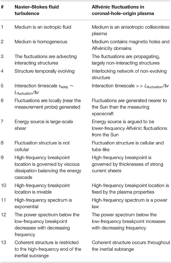
Table 2. A summary of differences between the Navier–Stokes turbulence in the wind tunnel and the Alfvénic fluctuations of the fast solar wind.

Similarities and Differences in the Fluctuations

In the Navier–Stokes wind tunnel, the fluctuations δv are interacting, “advecting” perturbations with a spatial pattern that evolves with time. Historically, the fluctuations have been described as eddies with a range of spatial scales (Tennekes and Lumley, 1972 sect. 8.2; Frisch, 1995 sect. 7.3); however, there are also coherent structures in the turbulence such as vortex filaments (e.g., Belin et al., 1996; Jimenez and Wray, 1998; Biferale et al., 2010). The eddies are thought to strongly interact with each other, particularly eddies of similar spatial scales, producing eddies of smaller spatial scale during the interaction; those eddy–eddy interactions (along with intermittent-structure interactions) create a cascade of flow kinetic energy from large scales to smaller scales (e.g., Argoul et al., 1989; Ch. 6 of Pope, 2000). Stretching of vorticity structures, important for both Navier–Stokes and MHD (e.g., Figure 8.4 of Tennekes and Lumley, 1972 or Moffatt, 2014), is dominant in the eddy–eddy interactions. Because of the cascade of energy, driving must be present for the Navier–Stokes turbulent fluctuations to persist.

In the Alfvénic solar wind, the fluctuations δv and δB are non-interacting, “propagating” perturbations with a spatial pattern that does not evolve. Figure 7.1 of Parker (1979) sketches a volume of tangled magnetic field embedded in a uniform field of strength B_o. If the plasma is incompressible, Parker points out that if there are field-aligned flows everywhere within the magnetic structure, then the volume of tangled magnetic field will propagate at the mean-field Alfvén speed B $_{o} / {(4 π ρ)}^{1 / 2}$ without distortion. Inside the volume, the total field is (B $_{o}^{2}$ + B $_{1}^{2}$ )^1/2, which is greater in strength than B_o, and so the Alfvén speed measured inside the volume B/(4πρ)^1/2 is greater than the mean-field Alfvén speed B $_{o} / {(4 π ρ)}^{1 / 2}$ , and so the magnetic structure moves at a speed lower than the Alfvén speed measured inside the structure. Borovsky J. E. (2020a) and Nemecek et al. (2020) have developed methodologies to find the moving reference frame of the solar-wind magnetic structure relative to the solar-wind plasma; at 1 AU, they find that the magnetic structure propagates at about 0.7 v_A along the Parker-spiral direction relative to the proton plasma of the solar wind, where v_A is the local Alfvén speed within the magnetic structure. In Figure 2 of Borovsky J. E. (2020a), the velocity of the magnetic structure is plotted as a function of time for Flattop 15. In 1-min resolution measurements of magnetic fluctuations at 1 AU, the angular spread of magnetic-field directions about the Parker-spiral direction is about 40° (cf. row 1 of Table 1 in Borovsky, 2010a). Hence, B₁ = B_o tan(40°) = 0.84 B_o. Thus, B = (B $_{o}^{2}$ + B $_{1}^{2}$ )^1/2 = 1.3 B_o, and so the structure moving at the Alfvén speed of B_o moves at about 1/1.3 = 0.77 times the measured Alfvén speed of B. In the reference frame of the magnetic structure, the proton flow vector v is everywhere parallel to the local magnetic field B, and the flow components in the structure change as the field direction spatially varies in the magnetic structure. Note, however, that the α-particle “beam” of the solar wind is approximately at rest in the reference frame of the magnetic structure (Nemecek et al., 2020). In the reference frame of the magnetic structure, the magnitude of the perpendicular component of the plasma flow vector is consistent with measurement error: the magnitude of the measured values of v_⊥ is consistent with a purely parallel-to-B velocity v_|| and the uncertainty in the parallel-to-B vs. perpendicular-to-B directions owing to the angular variation of the direction of B during the time required to obtain a vector v measurement. Such perpendicular-to-B flows would signify an evolution of the propagating magnetic structure, but the measurements do not support the observation of evolution. Note that measurements of the third-order Elsasser moments show evidence of an evolution of the Alfvénic fluctuations of the fast solar wind indicated by a non-zero energy-cascade rate in the fluctuations (e.g., Sorriso-Valvo et al., 2007; MacBride et al., 2008; Stawarz et al., 2010; Podesta, 2011).

There are two other aspects of the solar-wind Alfvénic fluctuations that differ from the Navier–Stokes fluctuations. The parallel-to-B flow of plasma in the reference frame of the magnetic structure gives rise to (1) flow jets at magnetic switchbacks, which produce (2) a solar-wind speed that has a skewed distribution. In the reference frame of the magnetic structure, the proton flow is toward the Sun: at locations where there are localized magnetic-field foldings (denoted as switchbacks or field reversals), the flow is anti-Sunward in the reference frame of the magnetic structure. Going to the reference frame of a spacecraft, which sees the magnetic structure moving outward along the Parker-spiral direction, the spacecraft will see a faster proton flow velocity in the magnetic-field switchback than in the surrounding regions: this localized fast flow gives the impression of a flow jet (Kahler et al., 1996; Balogh et al., 1999; Neugebauer and Goldstein, 2013; Borovsky, 2016; Borovsky J. E., 2020d). As seen by a spacecraft, the solar-wind bulk flow velocity depends on the direction of the magnetic field. This gives rise to the phenomena of one-sided variations of the solar-wind speed (Gosling et al., 2009; Matteini et al., 2014).

These differences are noted in Table 2 as items 3 and 4.

In the wind tunnel data, the pattern of evolving fluctuations is advected past the probe at a large velocity v_o ~ 12δv. In the WIND spacecraft measurements of Flattop 15, the pattern of Alfvénic fluctuations is advected past the probe at a large velocity v_o ~ 21δv.

The Navier–Stokes wind-tunnel turbulence fluctuations are characterized by a velocity perturbation δv on a mean flow v_o, whereas the Alfvénic solar-wind fluctuations are characterized by a velocity perturbation δv and magnetic-field perturbation δB on a mean flow v_o and mean magnetic-field vector B_o. In the Alfvénic fluctuations, δB(t) and δv(t) are highly correlated (for a toward-the-Sun mean magnetic field direction) or highly anticorrelated (for an away-from-the-Sun mean magnetic field-direction). In the full Flattop-15 data set, the 3-s data correlation coefficients are R_corr = 0.847 for v_x↔B_x, 0.880 for v_y↔B_y, and 0.888 for v_z↔B_z, using 15-s changes in the vectors. For Alfvénic fluctuations, it is convenient to describe v and B in terms of the outward-propagating and inward-propagating Elsasser variables Z_out = + sb and Z_in = v – sb, where b = B/(4πρ)^1/2 is the magnetic-field vector normalized to the Alfvén speed and the sign s = −1 for toward magnetic sectors and s = +1 for away magnetic sectors. The Alfvénic fluctuations of the fast solar wind are described by Z_out, with the values of Z_in in the noise of the v and B measurements (Wang et al., 2018).

An important difference between the turbulent fluctuations in the wind tunnel and the Alfvénic fluctuations propagating outward in the fast solar wind at 1 AU is that the wind-tunnel fluctuations are locally generated near the measurement location, whereas the Alfvénic fluctuations have been generated closer to the Sun and propagated to the measuring spacecraft at 1 AU. It is argued that the source of channel-flow fluid turbulence is large-scale shear in the flow (cf. Ch. 7 of Pope, 2000); in the solar wind, it has been argued that the energy source of the inertial-range turbulent fluctuations is lower-frequency outward-propagating Alfvénic fluctuations that originate at the Sun (Horbury et al., 1996; Zank et al., 1996; Smith et al., 2001; Vasquez et al., 2007; Bruno et al., 2019). These differences are noted in Table 2 as items 6 and 7.

Four other differences between the solar-wind Alfvénic fluctuations and the Navier–Stokes turbulent fluctuations are described in the following four paragraphs.

(1) The pattern of fluctuations in the solar wind represents a cellular spatial structure wherein the magnetic field undergoes a strong directional change across a “directional discontinuity” (strong current sheet) and then the magnetic-field directional variations are relatively small for an interval of time until another directional discontinuity is crossed. This pattern represents a magnetic cellular structure or flux-tube structure of the plasma wherein the directional discontinuities (current sheets) are the cell walls, and the intervals of small directional changes are the interiors of the cells (cf. Bruno et al., 2001; Borovsky, 2008). The fact that the flux-tube walls of the solar wind also coincide with intensity changes of the intensity of the solar-wind electron heat flux (electron Strahl) (Borovsky J. E., 2020b) implies that the flux-tube structure has a long-distance coherence going from 1 AU back toward the Sun. In the Alfvénic solar wind, the velocity fluctuations also have this cellular spatial structure because, in the reference frame of the magnetic structure, all flow velocities are parallel to B (Borovsky J. E., 2020a). This is noted in Table 2 as item 8.

(2) The solar-wind Alfvénic fluctuations exhibit matching pairs of current sheets wherein the field and flow vectors B(t) and v(t) are quasi-steady with a particular orientation, then B and v both undergo a sudden change in orientation across a first current sheet, and then after an interval of time, B and v suddenly return to their original orientations across a second current sheet. Two examples of this appear in Figure 2 [and other examples can be found in the literature (e.g., Gosling et al., 2011; Arnold et al., 2013)]. The event in the left-hand panel has a total duration of 16 s (from the first current sheet to the matching current sheet), with 144 s of data plotted. The event in the right-hand panel has a total duration of 5.5 min with 12 min of data plotted. The velocity components measured by the WIND spacecraft are plotted in red, and the magnetic-field components b (normalized to the Alfvén speed b = B/(4πρ)^1/2) are plotted in blue. In all panels, the locations of the two current sheets are marked with green arrows. Note the strong correlations in the temporal behaviors of v and B (that is what is meant by the fluctuations being “Alfvénic”). In both panels, the v and B vectors have the same orientations before current sheet “1” and after current sheet “2,” but different orientations between the current sheets. Such matching pairs of current sheets are common in the Alfvénic fluctuations of the fast solar wind and lead to a statistically non-randomness of the temporal changes of the magnetic-field direction at 1 AU (cf. Figure 10 of Borovsky J. E., 2020c).

(3) The fast Alfvénic plasma of coronal-hole origin exhibits “domains of Alfvénicity” wherein the v(t) ↔ B(t) correlation coefficient is very high for a temporal interval, then a non-Alfvénic (poorly correlated) transition of v and B occurs, and then another subsequent highly correlated v(t) ↔ B(t) temporal interval commences. For Flattop 15, the domains of Alfvénicity are plotted in Figure 14 of Borovsky (2016). At 1 AU, typical durations of a single domain are a few hours. These domains of Alfvénicity seen in coronal-hole-origin solar wind may be associated with open flux funnels in the downflow lanes at the edges of supergranules on the Sun (Dowdy et al., 1987; Tu et al., 2005; Peter, 2007; Kayshap et al., 2015), or they might be associated with magnetic separatrices in the corona (Burkholder et al., 2019). This is noted in Table 2 as item 2.

(4) The fast solar wind also exhibits magnetic holes (Turner et al., 1977; Winterhalter et al., 2000; Neugebauer et al., 2001; Amariutei et al., 2011), which are spatial regions of various sizes wherein the magnetic-field strength is locally much reduced from the average value. In most of the Alfvénic fluctuations of the solar wind, the direction of the magnetic-field vector B can vary by up to 180°, whereas the strength of the magnetic field B_mag essentially does not vary. Figure 3 shows an example of a magnetic hole in Flattop 15. Figure 3A plots the magnetic-field strength (blue), the Alfvén speed (green), and the proton-beta β_p = 8πnk_BT_p/B² (red) as functions of time for 9 min of observations. Figure 3B plots the magnetic pressure B²/8π, the proton pressure nk_BT_p, and the electron pressure nk_BT_e, with the electron properties measured by the SWE (Solar Wind Experiment) instruments (Ogilvie et al., 1995) onboard the WIND spacecraft. Note in Figure 3B the hint of pressure balance at the magnetic hole where the magnetic pressure is decreased within the magnetic hole and the particle pressures are increased. In Fourier analysis of the B_mag(t) time series and of the number density n(t) time series, magnetic holes contribute Fourier power to the spectral density where the interpretation of the Fourier power is the degree of compressibility of the solar-wind fluctuations (e.g., Marsch and Tu, 1990b; Goldstein and Roberts, 1999), but the true origin of the power is not in compressions or rarefactions. Note that a magnetic hole with a timescale τ contributes Fourier power at all frequencies. Likewise, magnetic holes make contributions to other B_mag and n statistics where they can be interpreted as compressions (Hnat et al., 2005; Matteini et al., 2018). The origins of magnetic holes are not known, and it is a matter of choice to consider them to be a property of the fluctuations (this section) or a property of the medium (Similarities and Differences in the Medium). This difference is noted in Table 2 as item 2. As pointed out in Borovsky J. E. (2020d), the descriptor “compressible” might be more accurately replaced by “inhomogeneous”.

FIGURE 2

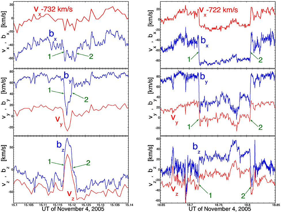
Figure 2. Two examples of paired current sheets, one with an event duration of 16 s (left panel) and one with a duration of 5.5 min (right panel). The velocity (red curves) is measured with 3-s time resolution and the magnetic field (blue curves) is measured with 0.09375-s time resolution. The two current sheets marking the beginning and end of the event are indicated in each panel with green arrows.

FIGURE 3

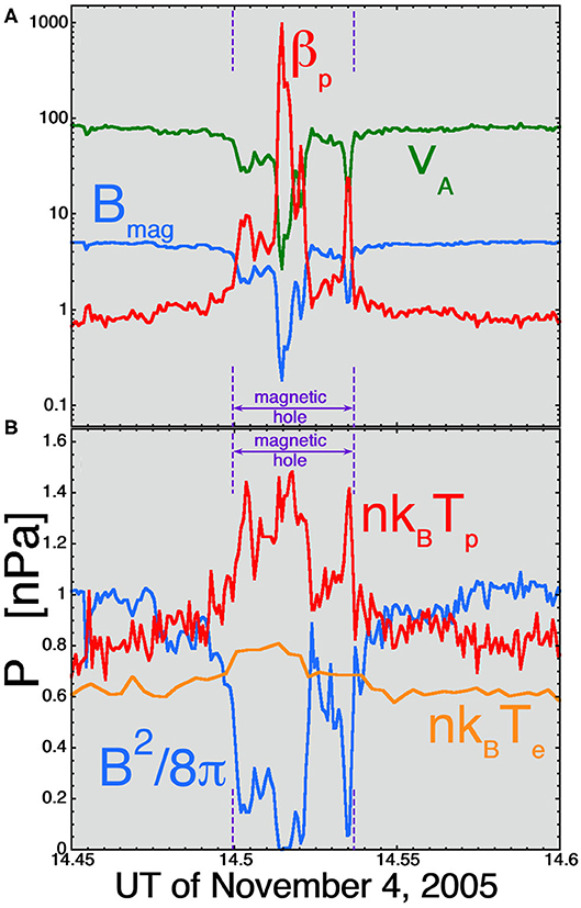
Figure 3. An example of a magnetic hole (denoted in purple) during Flattop 15. Nine minutes of WIND spacecraft data [plasma properties in panel (A) and pressures in panel (B)] are plotted, and the duration of the magnetic hole as seen by WIND was 130 s.

Similarities and Differences in the Fourier Spectra

In Figure 4, the power spectral densities for the streamwise velocity in the ONERA wind tunnel (Figure 4A), the radial proton-plasma velocity component of the solar wind in Flattop 15 (Figure 4B), and the radial component of the solar-wind magnetic field (Figure 4C) are plotted. The power spectral densities are calculated from the time series of measurements using the periodogram method (Cooley et al., 1970; Otnes and Enochson, 1972), with the power spectral density being the square of the Fourier transform. Data that are not a factor of 4 below the Nyquist frequency are not plotted. Data gaps in the time series are linearly interpolated.

FIGURE 4

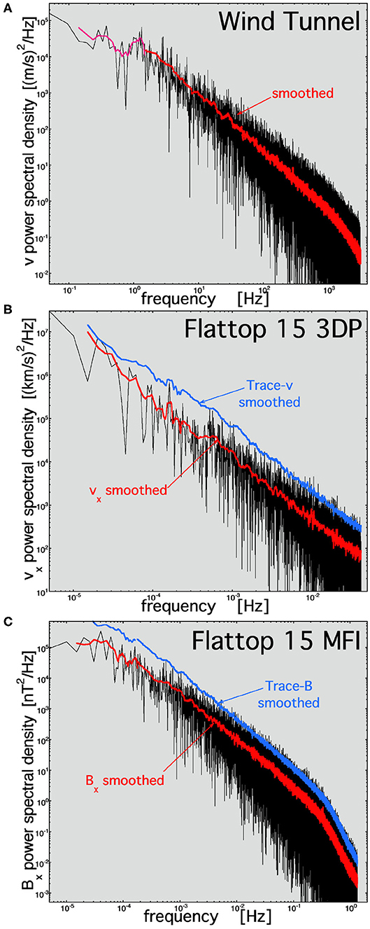
Figure 4. Periodogram power spectral densities for (A) the streamwise velocity v in the wind tunnel Navier–Stokes turbulence, (B) the radial (from the Sun) velocity v_x for the Alfvénic solar wind fluctuations of Flattop 15, and (C) the radial component of the magnetic field B_x for the Alfvénic solar wind fluctuations of Flattop 15.

The Inertial Subrange

In Figure 4A, the inertial subrange of the Navier–Stokes turbulence spans the frequency range from about 1 to 1,250 Hz, and in Figures 4B,C, the inertial subrange of the Alfvénic solar-wind fluctuations spans the frequency range from about 10⁻⁴ Hz (or lower) to 0.3 Hz.

Both the Navier–Stoke turbulence and the Alfvénic solar wind have power spectral densities that are power laws in the inertial subranges. In Table 3, the power-law spectral slopes for the spectra plotted in Figure 4 are collected, with information about the frequency range used for the power-law fits.

TABLE 3

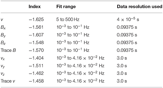
Table 3. Spectral fits in the inertial subrange.

The power-law spectral index of Navier–Stokes turbulence is well-known to be associated with a cascade of fluctuation energy from larger-scale size fluctuations to smaller-scale size fluctuations (cf. section 8.3 of Tennekes and Lumley, 1972; section 5.1 of Frisch, 1995). A power-law spectrum is interpreted as scale invariance or scale similarity (e.g., section 7.3 of Frisch, 1995).

In the Alfvénic solar wind, the inertial-range spectral index of the magnetic power spectral density and the inertial-range spectral index of the velocity power spectral index differ, with the velocity spectra being systematically shallower than the magnetic spectra (Podesta et al., 2007; Tessein et al., 2009; Borovsky, 2012). The amplitude and the spectral slope of the solar-wind magnetic power spectral density in the inertial range is determined by the amplitudes and occurrence distribution of strong current sheets (directional discontinuities) in the solar-wind plasma (Siscoe et al., 1968; Sari and Ness, 1969; Borovsky, 2010b), which are coherent structures. Because δv and δB are strongly correlated in the Alfvénic solar wind and because strong velocity shears occur at the sites of strong current sheets, it is almost certainly the case that the amplitude and the spectral index of the velocity power spectral density of the Alfvénic solar wind will be determined by the amplitudes and occurrence distribution of intense velocity shears in the solar-wind plasma. The strength of the contribution of coherent structures in the Navier–Stokes turbulence to the Navier–Stokes inertial-range power spectral density is not known.

The energy-transfer timescale in Navier-Stokes turbulence goes as the eddy turnover time τ_eddy = L_eddy/δv, where L_eddy is a large-eddy scale size at the low-frequency end of the inertial subrange, and δv is the rms level of velocity fluctuations (cf. Section 7.1 of Frisch, 1995). τ_eddy is the evolution timescale (lifetime) of a large eddy. The evolution timescale for the Alfvénic solar-wind fluctuations can be gauged as τ_evol ~ L_⊥/δv_⊥ where L_⊥ is the perpendicular-to-B fluctuation scale size, and δv_⊥ is the perpendicular-to-B fluctuation velocity. In the reference frame moving with the collective magnetic-field structure, v_⊥ is quite small, in the noise of the velocity measurements (Borovsky J. E., 2020a. Hence, the evolutionary timescale τ_evol of the Alfvénic fluctuations is long, much longer than an “eddy turnover time.” This is akin to the Elsasser-mode evolution timescale for the evolution of outward Elsasser fluctuations τ^out_L ~ L/δZⁱⁿ_L (Bruno and Carbone, 2016) where the amplitude δZⁱⁿ_L of the inward Elsasser fluctuations is in the noise of the measurements. This difference is noted in Table 2 as item 5.

The High-Frequency Breakpoint

Both Navier–Stokes turbulence and the Alfvénic solar wind have breakpoints in their power spectral densities defining the high-frequency end of the inertial subrange, with the power spectra steepening above the breakpoint.

For Navier–Stokes turbulence, the breakpoint is known to be associated with the cascade of energy to smaller spatial scales encountering stronger viscous dissipation of fluctuations at smaller spatial scales. This balance at the breakpoint is at the Kolmogorov dissipation scale. In Navier–Stokes turbulence, the breakpoint frequency (or wavenumber) is movable: if the turbulence is driven harder, the breakpoint moves to higher frequencies.

For solar-wind power spectra, the location of the high-frequency breakpoint is fixed by characteristic scale sizes in the solar-wind plasma: the ion gyroradius and the ion-inertial length (Leamon et al., 1998; Gary, 1999; Gary and Borovsky, 2004, 2008; Bruno and Trenchi, 2014). If the turbulence is driven harder, the frequency (wavenumber) of the breakpoint does not move. These characteristic plasma scale sizes represent a transition from fluid-like behavior at large scales to particle-kinetic behavior at small scales. It is known that the frequency of the high-frequency breakpoint in the magnetic power spectra of the Alfvénic fast solar wind is governed by the thicknesses of strong current sheets in the solar-wind plasma (Borovsky and Podesta, 2015), another strong effect of coherent structure on the power spectral density of the solar wind.

This difference is noted in Table 2 as items 9 and 10.

The frequency spectrum above the high-frequency break tends to be exponential-like for Navier–Stokes turbulence (e.g., section 8.4 of Tennekes and Lumley, 1972; Sirovich et al., 1994). For the Alfvénic fluctuations of the solar wind, the frequency spectrum above the high-frequency breakpoint tends to be a power law (cf. Figure 4B; Leamon et al., 1998; Alexandrova et al., 2009; Podesta, 2010; Sahraoui et al., 2010; Chen et al., 2014; Bruno et al., 2017). For Flattop 15, the fitted magnetic spectral indices in the 0.5- to 1.333-Hz frequency range above the breakpoint are −3.39 for B_x, −3.62 for B_y, −3.78 for B_z, and −3.66 for trace B. The shape and amplitude of the magnetic power spectral density above the high-frequency breakpoint are consistent with the Fourier spectra of individual solar-wind current sheets (Borovsky and Burkholder, 2020), suggesting that the high-frequency spectra may be governed by the spatial profiles of the solar-wind current sheets or by physical processes ongoing within the current sheets. The origin of the solar-wind high-frequency spectrum is an ongoing research issue, with dissipation, mode conversion, and current-sheet physics being considered (e.g., Podesta et al., 2010; Gary et al., 2012; Podesta and Borovsky, 2016; Mallet et al., 2017). This difference is noted in Table 2 as item 11.

The Low-Frequency Energy Subrange

At low frequencies, the power law of the inertial subrange ends.

In Navier–Stokes turbulence, the power spectrum rolls over and decreases in amplitude as f → 0 (e.g., Figure 5.7 of Frisch, 1995; Figure 6.20 of Pope, 2000). The end of the inertial range at low frequency is associated with a large-eddy scale size, usually a fraction of the width of the flow channel. The rolling over of the spectrum indicates an absence of energy in large-spatial-scale (low-frequency) fluctuations.

For fluctuations in the Alfvénic solar wind, the power spectrum at the low-frequency end of the inertial subrange bends to a shallower spectrum that is often characterized by a power-law index. The Alfvénic solar wind power spectrum increases in amplitude as f → 0. In long streams of coronal-hole-origin plasma, it is observed that the magnitude of the magnetic-field strength B_mag stays approximately constant (with the exception of magnetic holes). For the observed Alfvénic fluctuations, δv is correlated with δB such that δv ≈ ± v_AδB/B_mag (with the + sign for toward magnetic sectors and the – sign for away magnetic sectors). In the magnetic power spectral density, the amplitude δB is larger at lower frequencies. Eventually, going toward lower frequencies a point in the power spectra is reached where δB ≈ B_mag. The amplitudes δB of fluctuations at frequencies lower than this point saturate at δB ≈ B_mag (Villante, 1980; Matteini et al., 2018; Bruno et al., 2019), and this part of the power spectrum can have a spectral index near f ⁻¹, which is fluctuations with the same amplitude but with longer scale sizes (longer periods). The velocity fluctuations also saturate at δv ≈ v_A because they are tied to the magnetic-field fluctuations. Such a low-frequency saturation does not occur in Navier–Stokes turbulence. Certainly, at periods longer than about 1 day, the solar-wind power spectrum is dominated by surface features on the rotating Sun, with the differing surface features producing plasma with differing properties and differing magnetic structure (e.g., Matthaeus et al., 2007; Borovsky, 2018). It is often argued that the low-frequency energy-subrange outward propagating Alfvénic fluctuations are the energy source for the inertial-range Alfvénic fluctuations (Horbury et al., 1996; Zank et al., 1996; Smith et al., 2001; Vasquez et al., 2007; Bruno et al., 2019; but see Tu and Marsch, 1995 for a contrary argument).

This difference is noted in Table 2 as item 12.

Similarities and Differences in the Statistics of Derivatives

First and second time derivatives of the wind-tunnel and Flattop-15 time series are calculated over timescales Δt. The first derivative of a function f (t) is calculated as df /dt = [f(t + 0.5Δt) – f (t – 0.5Δt)]/ Δt, and the second derivative of f (t) is calculated as d²f /dt² = [–(1/3)f (t – Δt) + (16/3)f (t – 0.5Δt) – 10f (t) + (16/3)f (t + 0.5Δt) – (1/3)f (t – Δt)]/ Δt². The occurrence distributions of the first and second time derivatives of each time series will be compared with the occurrence distributions of the first and second time derivatives of a corresponding phase-randomized time series. The phase-randomized time series are created by (1) Fourier transforming the original time series, (2) randomizing the phase of each Fourier sine-cosine pair while preserving the amplitude, and (3) inverse Fourier transforming the randomized-phase Fourier transform. This process preserves the power spectral density of the time series (as approximated by the periodogram) and approximately preserves the autocorrelation function, which is the Fourier transform of the power spectral density. Examples of the original time series (blue curves) and a corresponding phase-randomized time series are plotted in the three panels of Figure 5. Note that a phase-randomized time series differs according to the random numbers chosen. Figure 5A plots 0.5 s of wind-tunnel velocity measurements, and Figures 5B,C plot 2 h of solar-wind measurements: these durations are a few correlation times. In Figures 5B,C note the strong correlation between the blue v_x and B_x curves (similar jumps, maxima, and minima) of the original time series.

FIGURE 5

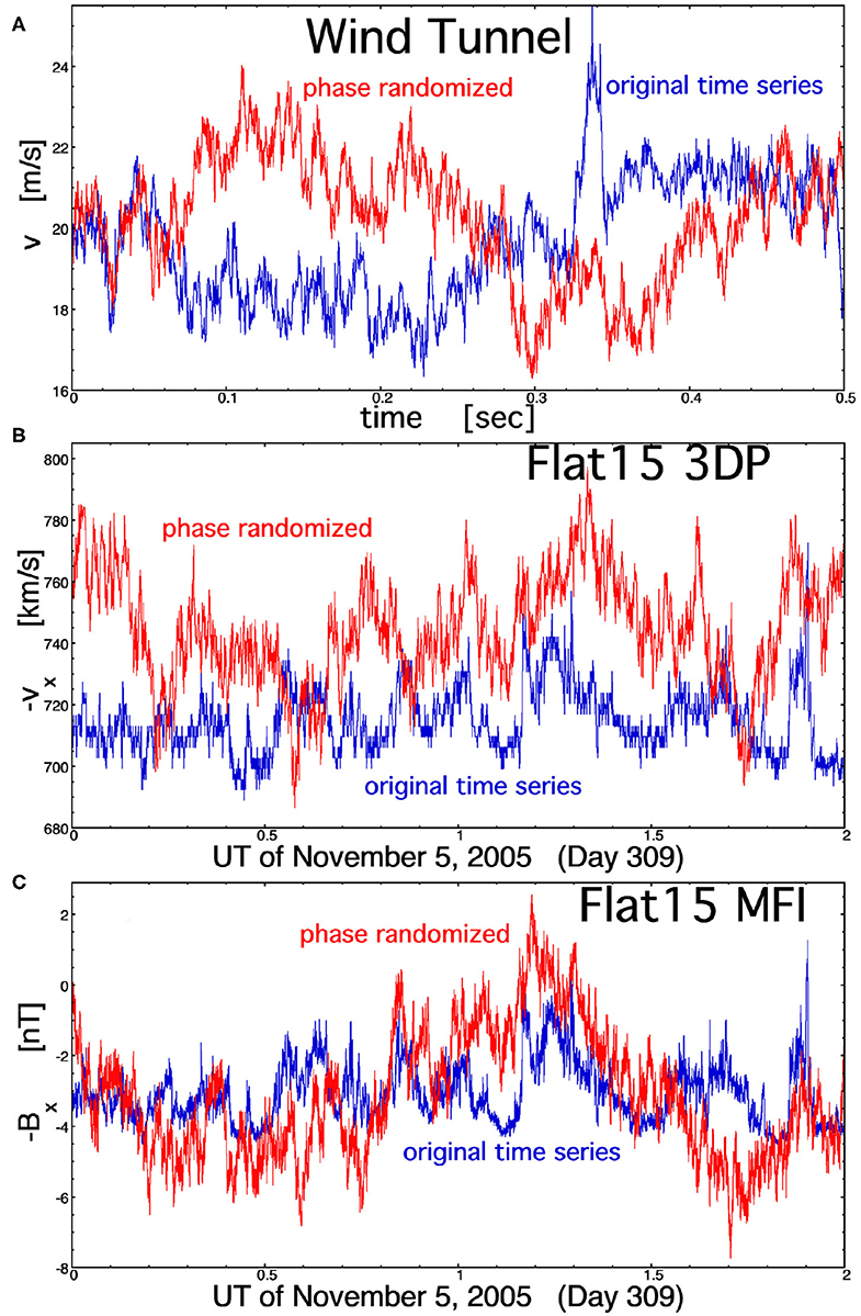
Figure 5. Comparisons of the measurement time series (blue curves) with randomized-phase versions of the time series for (A) the streamwise velocity v in the wind tunnel Navier–Stokes turbulence, (B) the radial (from the Sun) velocity v_x for the Alfvénic solar wind fluctuations of Flattop 15, and (C) the radial component of the magnetic field B_x for the Alfvénic solar wind fluctuations of Flattop 15. The time duration plotted in each panel is a few correlation times.

Figure 6 bins time derivatives over a timescale Δt that corresponds to a frequency just below the high-frequency breakpoint of the Fourier power spectral density: Δt = 3.2 × 10⁻³ s for the wind tunnel and Δt = 6 s for the solar wind. These derivatives will correspond to the high-frequency end of the inertial range. In each panel of Figure 6, the black curve is the occurrence distribution of the absolute values of the derivatives measured in the wind-tunnel v, Flattop-15 v_x, and Flattop-15 B_x time series. The red curve in each panel of Figure 6 is the occurrence distribution of the absolute values of derivatives measured in the same time series after the Fourier phases of the time series have been randomized. Note in Figure 6 that the standard deviations of the distributions of first and second derivatives are the same for the phase-randomized time series as they are for the original time series. The distributions are plotted in a manner such that the width of the randomized distribution is about the same fraction of the horizontal axis in each panel. For the original time series, the kurtosis K of the distribution of signed derivatives (not the absolute values, which are plotted) is noted in each panel of Figure 6. Here, the kurtosis K of N-values of x is defined as K = [N⁻¹Σ (x_i – < x>)⁴]/[N⁻²Σ (x_i – < x>)²] – 3, where Σ is the sum of i from 1 to N. The red distributions of derivatives (corresponding to the phase-randomized data) are all approximately Gaussian. The Gaussian distributions have K ≈ 0. The distributions of |dv/dt| and |d²v/dt²| for the Navier–Stokes turbulence of the wind tunnel (black curves in Figures 6A,B) are exponentials, with a weak tail at the end of the exponential. This non-Gaussianity is an indication of coherent structure in the time series of the wind-tunnel turbulence (with coherence being destroyed by phase randomization). The distributions of |dv_x/dt|, |dB_x/dt|, |d²v_x/dt²|, and |d²B_x/dt²| of the Alfvénic fluctuations in the fast solar wind (black curves in Figures 6B,C,E,F are all double exponentials). The second exponentials associated with the larger values can be interpreted as derivatives measured at the locations of strong current sheets and velocity shears in the solar wind, and the first exponentials corresponding to smaller values can be associated with measures of derivatives away from the current sheets and velocity shears. Note in Figures 6B,C,E,F that the weaker derivatives away from the current sheets and velocity shears are not Gaussian, indicating coherent structures in addition to the coherent structures of the strong current sheets and velocity shears. In the panels of Figure 6, the kurtosis values of the Alfvénic fluctuations of the solar wind are significantly larger than the kurtosis values of the Navier–Stokes–turbulence fluctuations.

FIGURE 6

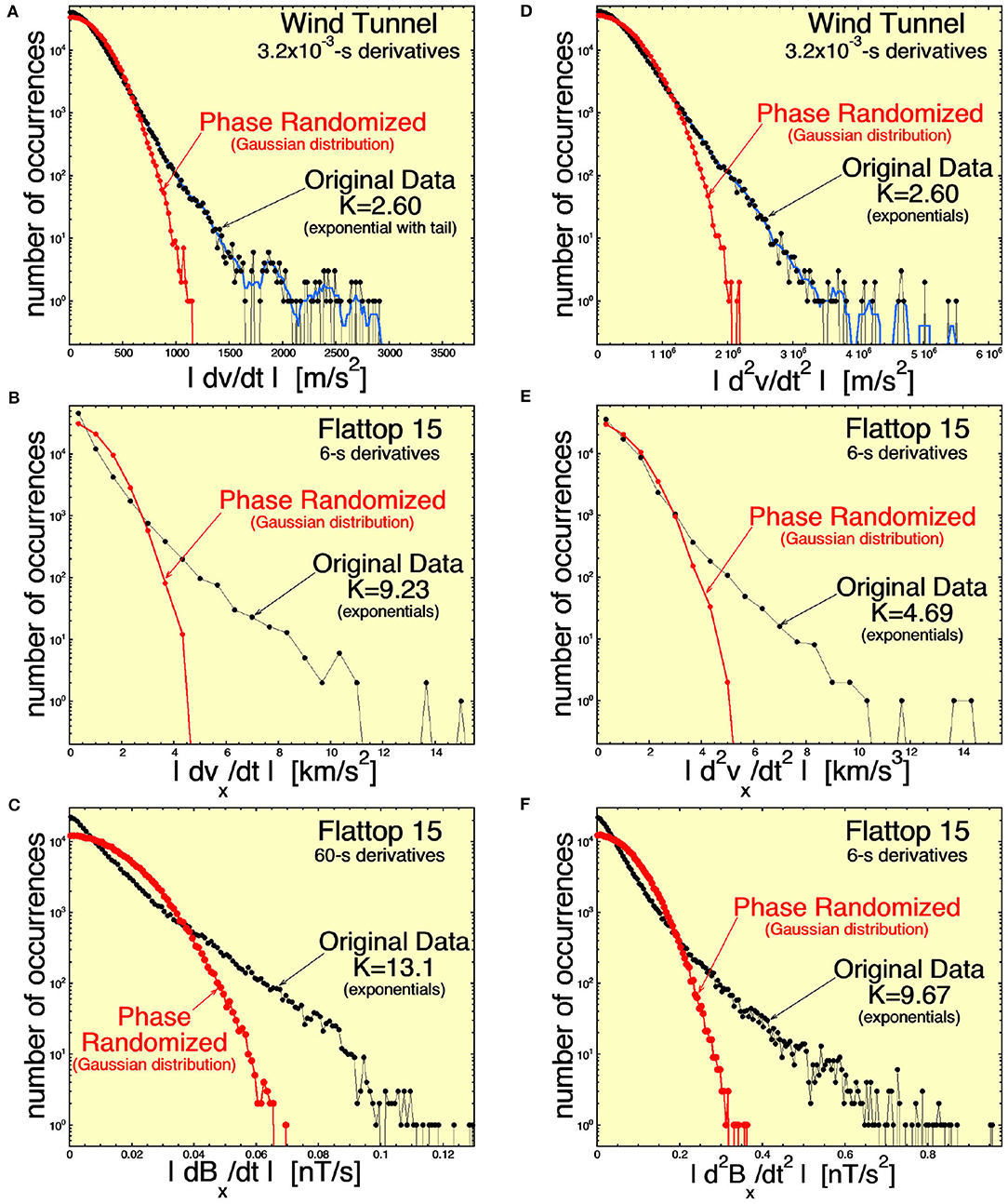
Figure 6. Distributions of the measured first time derivatives (A–C) and second time derivatives (D–F) for (A,D) the streamwise velocity v in the wind tunnel Navier–Stokes turbulence, (B,E) the radial (from the Sun) velocity v_x for the Alfvénic solar wind fluctuations of Flattop 15, and (C,F) the radial component of the magnetic field B_x for the Alfvénic solar wind fluctuations of Flattop 15. The black curves are time derivatives in the measured time series, and the red curves are time derivatives in phase-normalized versions of the measured time series. The time derivatives are over a timescale pertaining to the higher-frequency portion of the inertial subrange. For the original-data distributions, the kurtosis K of the signed values is noted.

In Figure 7, the Δt = 6-s first and second time derivatives are examined for the vector components of v and B in the Alfvénic solar wind of Flattop 15. The derivatives for each randomized-phase time series (all Gaussian distributions) are also plotted. Each component of v and of B exhibits double exponential distributions of the first and second derivatives.

FIGURE 7

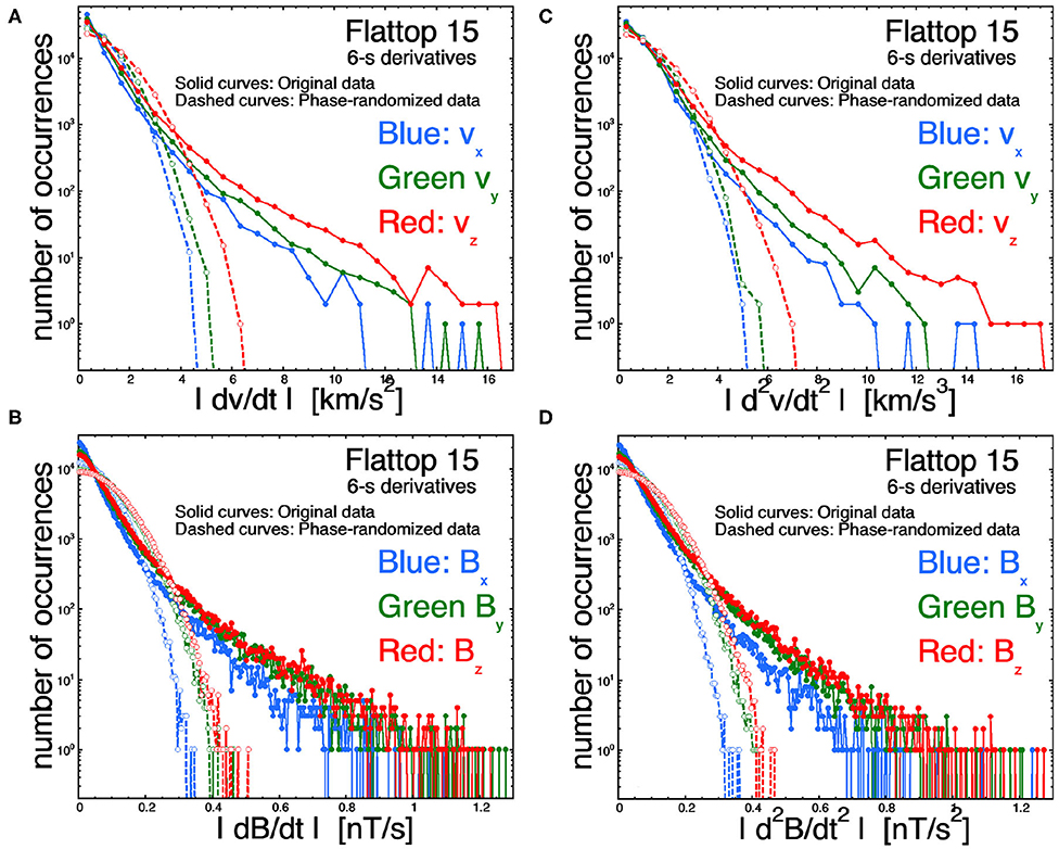
Figure 7. Distributions of the measured first time derivatives (A,B) and second time derivatives (C,D) for (A,C) the radial (from the Sun) velocity v_x for the Alfvénic solar wind fluctuations of Flattop 15, and (B,D) the radial component of the magnetic field B_x for the Alfvénic solar wind fluctuations of Flattop 15. As labeled in each panel, three solid curves are for the three components of the measured time series, and three dashed curves are for the phase-normalized versions of the measured time series.

In Figure 8, time derivatives are calculated over a timescale Δt that is 10 times longer than those in Figure 6 (Δt = 3.2 × 10⁻² s for the wind tunnel and Δt = 60 s for the solar wind), corresponding to a frequency that is 10 times lower, and in Figure 9, derivatives are calculated over a timescale that is 100 times longer (Δt = 0.32 s for the wind tunnel and Δt = 600 s = 10 min for the solar wind). The distributions of Figure 6 correspond to the high-frequency end of the inertial subrange, Figure 8 corresponds to a factor of 10 lower frequency than the high-frequency end, and Figure 9 corresponds to a factor of 100 lower frequency than the high-frequency end of the inertial subrange. In each panel of Figures 6, 8, 9, the black curve is the occurrence distribution of time derivatives in the original time series, and the red curve is the occurrence distribution of time derivatives in the corresponding phase-randomized time series. The red phase-randomized distributions are all Gaussian. Note also that the rms values of the black and red occurrence distribution in each panel are equal.

FIGURE 8

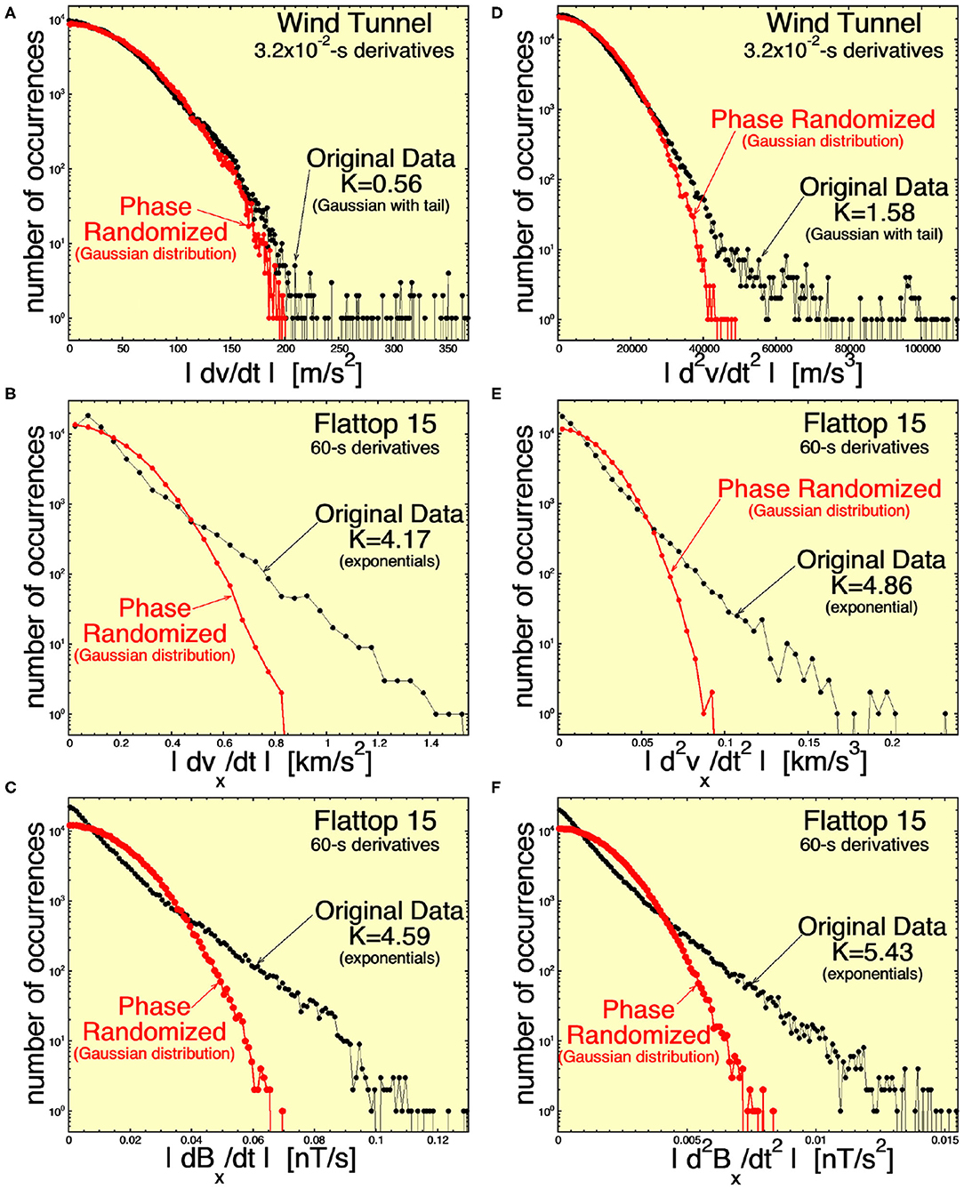
Figure 8. Similar to Figure 6, distributions of the measured first time derivatives (A–C) and second time derivatives (D–F) for (A,D) the streamwise velocity v in the wind tunnel Navier–Stokes turbulence (B,E) the radial (from the Sun) velocity v_x for the Alfvénic solar wind fluctuations of Flattop 15, and (C,F) the radial component of the magnetic field B_x for the Alfvénic solar wind fluctuations of Flattop 15. The black curves are time derivatives in the measured time series, and the red curves are time derivatives in phase-normalized versions of the measured time series. Here, time derivatives are over a timescale a factor of 10 longer than in Figure 6. For the original-data distributions, the kurtosis K of the signed values is noted.

FIGURE 9

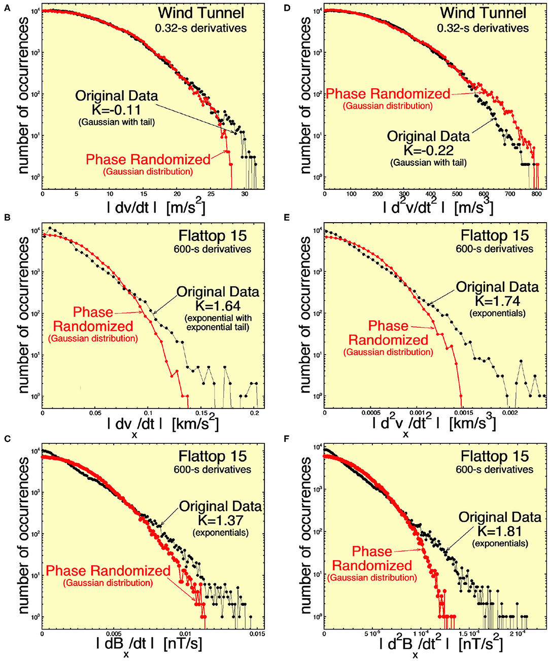
Figure 9. Similar to Figures 6, 8, distributions of the measured first time derivatives (A–C) and second time derivatives (D–F) for (A,D) the streamwise velocity v in the wind tunnel Navier–Stokes turbulence (B,E) the radial (from the Sun) velocity v_x for the Alfvénic solar wind fluctuations of Flattop 15, and (C,D) the radial component of the magnetic field B_x for the Alfvénic solar wind fluctuations of Flattop 15. The black curves are time derivatives in the measured time series, and the red curves are time derivatives in phase-normalized versions of the measured time series. Here time derivatives are over a timescale a factor of 100 longer than in Figure 6. For the original-data distributions, the kurtosis K of the signed values is noted.

Figure 6A finds that the |dv/dt| distribution for Navier–Stokes turbulence near the high-frequency end of the inertial subrange is exponential-like (with kurtosis of the signed values K = 2.60), indicating the presence of coherent structures. However, Figure 8A finds that the distribution of |dv/dt| a factor of 10 lower in frequency is approximately Gaussian (with K = 0.56 for the signed values of dv/dt), showing an absence of coherent structure with scale sizes a factor of 10 below the high-frequency end of the inertial subrange. Consistent with this, Figure 9A shows an absence of coherent structure in the |dv/dt|distribution at a frequency 100 times lower than the high-frequency end of the inertial subrange, with K = −0.11 for the signed values.

This lack of lower-frequency coherent structure is not the case for the first time derivatives of v_x and B_x in the Alfvénic fluctuations of the solar wind. Figures 8B,C, 9B,C, show persistent exponential distributions of |dv_x/dt| and |dB_x/dt| at 10 times and 100 times lower frequencies than the high-frequency end of the inertial subrange, with kurtosis values for the signed first derivatives that are strongly non-zero.

Similar cases are found examining the occurrence distributions of the second time derivatives in the right-hand columns of Figures 6, 8, 9. (1) There is an absence of coherent structure in the wind-tunnel Navier–Stokes turbulence at frequencies lower than the high-frequency end of the inertial subrange (although the disappearance of coherence is not as rapid going down in frequency as was the case for |dv/dt|); (2) the coherent structure as indicated by the |d²v_x/dt²| and |d²B_x/dt²| occurrence distributions persists to at least a factor of 100 below the high-frequency end of the inertial subrange (cf. Figures 9E,F).

These differences are noted in Table 2 as item 13.

Level Shifts and Calm Regions

As discussed in Similarities and Differences in the Fluctuations, the solar-wind plasma is characterized by a cellular spatial structure wherein the magnetic field undergoes a strong directional change across a “directional discontinuity” (strong current sheet), and then the magnetic-field directional variations are relatively small for an interval of time. In the Alfvénic solar wind, the velocity v, which is everywhere parallel to B in the reference frame of the magnetic structure, also has this cellular spatial structure (Borovsky J. E., 2020a). In the time series of the individual components of v or of B, the cell interiors appear as flat spots (with noise).

In Figure 10, running medians of the wind-tunnel v(t) time series and of the Flattop-15 B_x(t) time series are plotted. The running median of v(t) is over 4 × 10⁻³-s time intervals, and the running median of B_x(t) is over 16-s time intervals: each of these interval lengths corresponds to a frequency that is about a factor of 5 below the high-frequency breakpoints in their respective power spectral densities. The original time series is plotted in red, and the running medians are plotted in blue. The 2 s of wind-tunnel data plotted in Figure 10A is ~500 running-median interval lengths, and the 2 h of Alfvénic solar wind data plotted in Figure 10B is about 450 running-median interval lengths. The shifts in levels, resulting in “flat spots,” can be seen in the blue B_x running-median curve in Figure 10B.

FIGURE 10

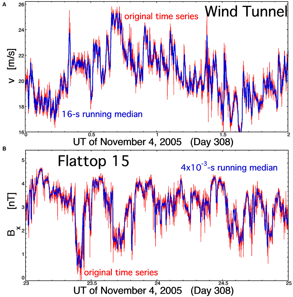
Figure 10. Running medians (blue curves) are compared with the measurement time series (red curves) for (A) the streamwise velocity v in the wind tunnel Navier–Stokes turbulence and (B) the radial component of the magnetic field B_x for the Alfvénic solar wind fluctuations of Flattop 15. The running medians are over timescales that are about five times longer than the period corresponding to the high-frequency breakpoints of the power spectral densities.

To gauge this effect in the Alfvénic solar-wind fluctuations relative to the Navier–Stokes turbulence, running medians of the time series are calculated, and then time differences in the running-median time series are statistically analyzed looking for an excess of small differences representing flat regions in the time series. The occurrence distributions of the time differences are plotted in Figure 11. The red curve is the occurrence distribution of 8-s changes in B_x(t) after the Flattop-15 B_x(t) time series is subjected to 16-s running medians. The running median of 16 s is approximately five times the period associated with the 0.3-Hz high-frequency breakpoint of the B_x power spectral density (cf. Figure 4C). The plotted occurrence distribution is normalized (horizontal axis) so that the root mean square of the distribution of differences is unity. For comparison, the blue curve in Figure 11 is the occurrence distribution of 2 × 10⁻³-s changes in v(t) after the wind-tunnel v(t) time series was subjected to a 4 × 10⁻³-s running median. The running median of 4 × 10⁻³ s is approximately five times the period associated with the 1,250-Hz high-frequency breakpoint of the wind-tunnel v power spectral density (cf. Figure 4A). Again, the blue plotted occurrence distribution is normalized so that the root mean square of the distribution of differences is unity. Figure 11 shows an excess of small differences in the distribution of B_x(t) changes in the Alfvénic fluctuations of the solar wind that are not seen in the v(t) changes of the Navier–Stokes turbulence. This excess indicates a prevalence of flat regions of the Alfvénic-fluctuation time series relative to the Navier–Stokes-turbulence time series. The excess of small differences in B_x(t) changes (cf. Figure 11) can also be seen if running averages are taken instead of running medians.

FIGURE 11

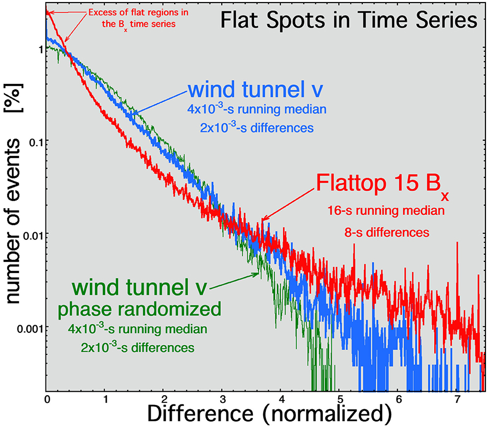
Figure 11. The normalized distribution of 2 × 10⁻³-s differences of the streamwise velocity v in the wind tunnel Navier–Stokes turbulence (blue curve) and the normalized distribution of the 8-s differences of the radial component of the magnetic field B_x for the Alfvénic solar wind fluctuations of Flattop 15 (red curve) calculated after 4 × 10⁻³-s and 16-s running medians were applied to the time series. The green curve is the normalized distribution of differences of the streamwise wind-tunnel velocity v after the wind-tunnel time series was (1) phase randomized and then (2) processed with a 4 × 10⁻³-s running median.

This difference is noted in Table 2 as item 8.

Summary and Discussion

As analyzed in the present study, similarities between the Alfvénic fluctuations of the fast (coronal-hole-origin) solar wind and Navier–Stokes turbulence are restricted to the well-known fact that both exhibit an inertial subrange with (1) a power-law functional form with similar spectral indices, (2) a high-frequency breakpoint, and (3) a low-frequency breakpoint. The differences discussed and found are summarized in Table 2; the differences cataloged in Table 2 pertain to the medium (1 and 2), to the physical nature of the fluctuations (3–8), and to the properties of the power spectral densities and statistics of the fluctuations (9–13). The extensive cataloging in Table 2 of differences between Navier–Stokes turbulence and the Alfvénic fluctuations of the coronal-hole-origin solar wind is unique to the present study. Difference 13 in Table 2 is a new finding.

An outstanding question is why would the inertial-range spectral properties of the outward-propagating Alfvénic fluctuations in the solar wind be similar to the properties of Navier–Stokes turbulence? A related question is how the outward-propagating structures obtained their properties? Three possibilities are suggested here. (1) Maybe the outward-propagating fluctuations are fossils of turbulence at the Sun in the sense that the structure seen in the inner heliosphere is the relaxation of an MHD turbulence near the Sun to an Alfvénic state (e.g., Dobrowolny et al., 1980; Matthaeus et al., 2008; Telloni et al., 2016). (2) Maybe the outward propagating fluctuations carry the signal of turbulent footpoint and/or reconnection motions in the corona. (3) Maybe the outward-propagating fluctuations carry the signatures of non-linear interactions that occurred when non-Alfvénic perturbations near the Sun propagate apart into non-evolving Alfvénic perturbations (cf. Section 7.1 of Parker, 1979). Note that Smith et al. (2009) and Stawarz et al. (2010) have suggested that an inverse cascade is ongoing to enforce the dominance of outward propagation in the fast solar wind.

In the present study, two distinct types of fluctuations were analyzed on equal footing with a few different analysis techniques. The differences in the fluctuation properties from the Navier–Stokes fluctuations cited in the present study are specific to the highly Alfvénic fluctuations in coronal-hole-origin plasma: for other types of solar-wind fluctuations in other types of solar-wind plasma, these specific properties and differences (e.g., Table 2) do not hold. For the future, there are more types of classical solar-wind data sets and more analysis techniques that can be applied. A future challenge would be to bring together experts in different analysis techniques to simultaneously analyze the various data sets that are characteristic of the different types of solar wind and the different types of solar-wind fluctuations. The two data sets used here are (1) Navier–Stokes turbulence in a wind tunnel and (2) Alfvénic fluctuations in the fast (coronal-hole-origin) solar wind. A third data set would be (3) Alfvénic fluctuations in the slow (streamer-belt-origin) solar wind (e.g., D'Amicis and Bruno, 2015; D'Amicis et al., 2016, 2019; Borovsky et al., 2019), and a fourth data set would be (4) non-Alfvénic slow wind. Candidate long-duration data sets are available in the collection of long pseudostreamer intervals of streamer-belt-origin solar wind that were collected to develop the Xu and Borovsky (2015) solar-wind plasma categorization scheme. A fifth data set would be (5) non-Alfvénic non-Parker-spiral sector-reversal-region plasma. There are long intervals of this plasma that have been collected for use in developing the Xu and Borovsky (2015) solar-wind categorization scheme. Among the analysis techniques that could be applied to each data set are (a) Fourier power-spectral analysis, (b) autocorrelation-function analysis, (c) third-order moments, (d) fractal and multifractal analysis, (e) compressibility analysis, (f) intermittency studies (wavelet, partial variance of increments), (g) running-median analysis, (h) dimensional analysis, (i) Taylor scale analysis, (j) fractional-derivative analysis, (k) zero-crossing analysis, (l) peak-valley counting statistics, (m) current-sheet orientation statistics, (n) event statistics, and (o) time-series clustering.

Data Availability Statement

Publicly available datasets were analyzed in this study. This data can be found here: https://cdaweb.gsfc.nasa.gov/index.html/.

Author Contributions

JB planned, outlined, researched, and drafted the manuscript. TM provided data analysis and mathematical expertise. All authors contributed to the article and approved the submitted version.

Funding

This work at the Space Science Institute was supported by the NSF SHINE program via award AGS-1723416, by the NASA Heliophysics Guest Investigator Program via grant NNX17AB71G, and by NASA Heliophysics LWS TRT program via grant NNX14AN90G.

Conflict of Interest

The authors declare that the research was conducted in the absence of any commercial or financial relationships that could be construed as a potential conflict of interest.

Acknowledgments

The authors thank Gian Luca Delzanno and Zdenek Nemecek for helpful conversations. Text files of the 4 × 10⁻⁵-s wind-tunnel measurements, the 3-s solar-wind velocity measurements, and the 0.09375-s solar-wind magnetic-field measurements used in this investigation are available at: Borovsky J. (2020, https://zenodo.org/record/3928592#.Xv4MPi2ZP2I).

References

Alexandrova, O., Saur, J., Lacombe, C., Mangeney, A., Mitchell, J., Schwartz, S. J., et al. (2009). Universality of solar-wind turbulent spectrum from MHD to electron scales. Phys. Rev. Lett. 103:165003. doi: 10.1103/PhysRevLett.103.165003

PubMed Abstract | CrossRef Full Text | Google Scholar

Amariutei, O. A., Walker, S. N., and Zhang, T. L. (2011). Occurrence rate of magnetic holes between 0.72 and 1 AU: comparative study of cluster and VEX data. Ann. Geophys. 29, 717–722. doi: 10.5194/angeo-29-717-2011

ORIGINAL RESEARCH article

Some Similarities and Differences Between the Observed Alfvénic Fluctuations in the Fast Solar Wind and Navier–Stokes Turbulence

Introduction

Similarities and Differences in the Medium

Similarities and Differences in the Fluctuations

Similarities and Differences in the Fourier Spectra

The Inertial Subrange

The High-Frequency Breakpoint

The Low-Frequency Energy Subrange

Similarities and Differences in the Statistics of Derivatives

Level Shifts and Calm Regions

Summary and Discussion

Data Availability Statement

Author Contributions

Funding

Conflict of Interest

Acknowledgments

References

This article is part of the Research Topic

People also looked at