Introduction to Numerical Relativity

1. Introduction

General Relativity is the theory that identifies gravity as the curvature of a four dimensional space-time manifold. The consequences of this identification deeply changed our conception of Nature. From the physics point of view, Relativity introduced new ideas, like that time and space are not absolute but depend on the observer, that the effects of gravity propagate at the speed of light, or that energy and matter are equivalent and can modify the structure of both space and time, among others. From the mathematical point of view, the main consequence is that gravity can be described by using the tools of differential geometry, where the basic object to represent a manifold is the metric g_ab that allow us to compute distances between neighboring points. The famous Einstein equations describe the dynamics of the four-dimensional space-time metric and how it is deformed by a given mass-energy distribution. On the other hand, the Bianchi identities from differential geometry ensure that the divergence of the Einstein tensor vanishes, implying the conservation of the stress-energy tensor (i.e., corresponding to energy and linear momentum conservation), which describes how matter moves in a curved spacetime.

One of the greatest achievements of General Relativity was the prediction of gravitational waves, space-time deformations produced by acceleration of masses which behave like waves as they propagate away from the sources. Gravitational waves are essentially unscattered between emission and detection, thereby giving direct information about the sources powering these phenomena. Precisely due to the weak interaction of these waves with matter, their existence was initially only confirmed indirectly by observations of the orbital dynamics of binary pulsars (Hulse and Taylor, 1975; Will, 2014). However, current kilometer-scale interferometric gravitational wave (GW) detectors, such as Advanced LIGO (aLIGO) (Abramovici et al., 1992) and Advanced Virgo (adVirgo) (Caron et al., 1997) facilities, since 2015 have directly detected gravitational waves on the kiloHertz frequency regime, consistent with the merger of binary black holes and binary neutron stars (Abbott et al., 2019). Further improvements on these detectors, as well as new ones added to the array of GW observatories, will allow to establish many routinary GW observations in the next few years. These new observations allow us a new way to study some of the most energetic and exotic processes in the universe and start a new era of gravitational wave astronomy that will inevitably lead to unprecedented discoveries and breakthroughs not only in Astrophysics and Cosmology, but also in fundamental theories like gravity and nuclear physics. The detection, identification, and accurate determination of the physical parameters of sources is crucial to validate (and challenge) not only our theories but also our astrophysical models, which rely both on precise experimental data and on the availability of template banks of theoretical waveforms. For the slow inspiral, when the neutron stars (NSs) or black holes (BHs) are widely separated, analytical approximations for the gravitational waveforms are provided by perturbative post-Newtonian (PN) expansion techniques (Blanchet, 2014). For the last orbits and merger, where the fields are particularly strong and most might be gained in terms of insight on fundamental physics, the PN expansion breaks down and the full Einstein equations have to be solved numerically. This has only become possible after a series of breakthroughs in the field of Numerical Relativity (Pretorius, 2005a; Baker et al., 2006b; Campanelli et al., 2006a), calling for an incorporation of this new type of information into data analysis strategies and methods. Since then, outstanding progress has been made to explore the late stage of binary coalescence with numerical methods. The next sections summarize some of the foundations of Numerical Relativity, with a view on the modeling of gravitational sources, from the construction of a well-posed evolution system to the numerical methods commonly employed to solve them. Notice that this review focus on Cauchy formulations, excluding other alternatives. For a wider overview of all the possible formulations, please see Lehner (2001).

2. Evolution Systems

2.1. Einstein Equations

The equations of motion of a classical theory like General Relativity can be derived directly from a suitable action by using the Euler-Lagrange equations, leading to the well-known Einstein equations (Misner et al., 1973),

$\begin{array}{ll}{G}_{ab}\equiv R_{ab}-\frac{R}{2}{g}_{ab}=8\pi T_{ab},& (1)\end{array}$

where G_ab is the Einstein tensor, R_ab is the Ricci tensor of the spacetime represented by the metric g_ab, $R\equiv g^{ab}{R}_{ab}$ is the Ricci or curvature scalar, and T_ab is the stress-energy tensor describing generically the matter-energy distributions in the spacetime. We have chosen geometric units such that G = c = 1 and adopt the convention where roman indices a, b, c, ... denote space-time components (i.e., from 0 to 3), while i, j, k, ... denote spatial ones (i.e., from 1 to 3).

The Ricci tensor can be written in terms of the Christophel symbols ${\Gamma }_{bc}^a$ as follows

$\begin{array}{l}{R}_{ab}\equiv {\partial }_c{\Gamma }_{ab}^c-{\partial }_a{\Gamma }_{cb}^c+{\Gamma }_{cd}^c{\Gamma }_{ab}^d-{\Gamma }_{da}^c{\Gamma }_{cb}^d,\\ {\Gamma }_{ab}^c=\frac{1}{2}{g}^{cd}({\partial }_a{g}_{bd}+{\partial }_b{g}_{ad}-{\partial }_d{g}_{ab}),& (2)\end{array}$

Notice that Equations (1–2) form a system of ten non-linear partial differential equations (PDEs) for the spacetime metric components g_ab, which are coupled to the matter fields by means of the stress-energy tensor.

On the other hand, an important relation in differential geometry, known as the (contracted) Bianchi identities, implies the covariant conservation law for the Einstein tensor and, consequently, for the stress-energy tensor,

$\begin{array}{lll}{\nabla }_a{G}^{ab}& =& 0\Rightarrow {\nabla }_a{T}^{ab}=0,\\ {\nabla }_a{T}^{ab}& =& {\partial }_a{T}^{ab}+{\Gamma }_{ac}^a{T}^{cb}+{\Gamma }_{ac}^b{T}^{ac}& (3)\end{array}$

where ∇_a is the covariant derivative, the generalization of the partial derivative on a manifold. These covariant equations correspond to conservation laws for both the energy and linear momentum, which are the basic physical equations to describe any matter field. Notice also that the Bianchi identities imply that four of the ten components of Einstein's equations cannot be independent. This redundancy gives rise to both the four coordinate degrees freedom and the four constraint equations, which will be clearly manifested in the 3+1 decomposition described in the next section.

2.2. The 3+1 Decomposition

Despite its elegance and compactness, the covariant form of the four-dimensional Einstein equations is not suitable to describe how the gravity fields evolve from an initial configuration toward the future. In such case, it is more intuitive to consider instead a time succession of three-dimensional spatial slice geometries, called foliation, where the evolution of a given slice is given by the Einstein equations (for more detailed treatments see for instance; Gourgoulhon, 2007; Alcubierre, 2008; Bona et al., 2009; Baumgarte and Shapiro, 2010; Shibata, 2015). This 3+1 decomposition, in which the four-dimensional manifold is splitted into “space+time” components and the covariant Einstein equations are converted into evolution equations for three-dimensional geometric fields, can be summarized in the following steps:

• specify the choice of coordinates. The covariance of Einstein equations implies that they can be written in the same generic way on any system of coordinates, which can be defined by a set of observers. The spacetime can be foliated by a family of spacelike hypersurfaces Σ, which are intersected by a congruence of time lines that will determine our observers (i.e., our system of coordinates). This congruence is described by the vector field t^a = αn^a+β^a, where n^a is the timelike unit vector normal to the spacelike hypersurfaces, α is the lapse function which measures the proper time of the Eulerian (orthogonal) observers and β^a is the shift vector that measures the displacement, between consecutive hypersurfaces, of the time line t^a followed by the observers with respect to the normal n^a (see Figure 1).

• decompose every 4D object into its 3+1 components. The choice of coordinates allows for the definition of a spatial projection tensor ${{\gamma }^a}_b\equiv {\delta }_b^a+n^a{n}_b$. Any four-dimensional tensor can be decomposed into 3+1 pieces using either the spatial projector to obtain the spatial components, or contracting with n^a for the time components. For instance, the line element measuring the distance between neighboring points can be written by using these generic 3+1 coordinates as

$\begin{array}{ll}d{s}^2=g_{ab}d{x}^{a}d{x}^b=-{\alpha }^{2}d{t}^2+{\gamma }_{ij}(d{x}^i+{\beta }^{i}dt)(d{x}^j+{\beta }^{j}dt),& (4)\end{array}$

where the spatial three-dimensional induced metric γ_ij is just the projection of the four-dimensional metric g_ab into the space-like hypersurface Σ. Other objects, like the stress-energy tensor, can also be decomposed into its various components, namely

$\begin{array}{ll}\tau \equiv T^{ab}{n}_a{n}_b,S_i\equiv -T_{ab}{n}^a{{\gamma }^b}_i,S_{ij}\equiv T_{ab}{{\gamma }^a}_i{{\gamma }^b}_j.& (5)\end{array}$

• write down the field equations in terms of the 3+1 components. Within the framework outlined here, the induced metric γ_ij is the only unknown, since both lapse and shift are set by our choice of coordinates. In differential geometry it is also common to define an additional tensor K_ij with a strong geometrical meaning, as it describes the change of the induced metric along the congruence of normal observers. This definition involves the Lie derivative ${{L}}_{\text{n}}$, a generalization of the directional derivative along the vector n in a manifold. Therefore, the definition of the extrinsic curvature and the 3+1 decomposition of Einstein equations form an hyperbolic-elliptic system of PDEs, commonly known as the Arnowitt-Deser-Misner (ADM) formalism (Witten, 1962; York, 1979), which can be written as

$\begin{array}{l}{K}_{ij}\equiv -\frac{1}{2}{{L}}_{\text{n}}{\gamma }_{ij}=-\frac{1}{2\alpha }({\partial }_t-{{L}}_{\beta }){\gamma }_{ij},\\ {{L}}_{\beta }{\gamma }_{ij}={\beta }^k{\partial }_k{\gamma }_{ij}+{\gamma }_{ik}{\partial }_j{\beta }^k+{\gamma }_{kj}{\partial }_i{\beta }^k,& (6)\end{array}$

$\begin{array}{l}\left({\partial }_t-{{L}}_{\beta }\right)K_{ij}=-{\nabla }_i{\nabla }_j\alpha +\alpha (R_{ij}-2K_i{}^k{K}_{jk}+\text{trK}{K}_{ij}\\ =-8\pi \left[S_{ij}-\frac{{\gamma }_{ij}}{2}\left(\text{trS}-\tau \right)\right]),& (7)\end{array}$

$\begin{array}{ll}{H}={R_i}^i+{(\text{trK})}^2-{K_i}^j{K_j}^i-16\pi \tau =0,& (8)\end{array}$

$\begin{array}{ll}{{M}}_i={\nabla }_j({K_i}^j-\text{trK}{{\delta }_i}^j)-8\pi S_i=0.& (9)\end{array}$

where we have defined the trace of any three-dimensional tensor C_ij as $trC={\gamma }^{ij}{C}_{ij}$. The evolution hyperbolic Equations (6,7) for the evolved fields {γ_ij, K_ij} are complemented with the energy and momentum constraint Equations (8,9), that have to be satisfied at each hypersurface. This system of equations needs to be completed with a specification of the coordinate system, that is, by a choice of lapse and shift {α, βⁱ}. The ADM formalism still preserves the covariance under spatial or time coordinate transformations (i.e., 3+1 covariance). Notice that, although manifest four-dimensional covariance is lost when performing the 3+1 decomposition, the solution space is still invariant under general coordinate transformations.

FIGURE 1

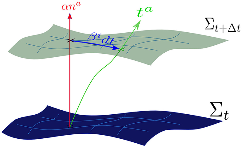
Figure 1. Foliation of the spacetime manifold. The lapse function α measures the proper time along the normal n^a to the hypersurface Σ_t, which is equipped with an induced metric γ_ij. The shift vector βⁱ measures the displacement, on consecutive hypersurfaces, between the observer time lines t^a and the normal lines n^a.

One can take advantage of the contracted Bianchi identities to prove that the constraint Equations (8,9) are just first integrals of the evolution ones (6,7), so that if the constraints are satisfied on an initial hypersurface (i.e., ${H}={{M}}_i=0$ at Σ_t), they will remain satisfied for all times. This redundancy of the equations allows for different evolution approaches. The most straightforward choice, the constrained evolution approach, involves solving simultaneously both the evolution equations and the constraints, but it presents several difficulties. From the theoretical point of view, it is not clear how to split the dynamical modes, solved through evolution equations, from the constrained ones, enforced by elliptic equations. From the computational point of view, elliptic equations are computationally more expensive and difficult to solve efficiently than hyperbolic ones. A simpler alternative is given by the free evolution approach, where the fields are obtained uniquely from the evolution equations, while the constraints are enforced only at the initial time (i.e., although they can be computed during the evolution to estimate the validity of the solution). Notice however that discarding the constraint equations breaks the underlying invariance of the solutions. Due to its simplicity, the free evolution approach has traditionally been the most common choice in Numerical Relativity applications without symmetry assumptions, particularly in efforts associated to the modeling of gravitational wave sources.

It is important to stress that any astrophysical scenario, except those including only black holes, involves some type of matter, which will evolve on a curved spacetime as described by Equation (3). We can also perform the 3+1 decomposition on this equation to obtain the evolution for the matter energy density τ and the momentum density S_i, namely

$\begin{array}{llll}\left({\partial }_t-{{L}}_{\beta }\right)\tau & +& \alpha {\nabla }_k{S}^k=\alpha \left(\tau trK-2S^k{\partial }_{k}ln\alpha +K_{ij}{S}^{ij}\right),& (10)\end{array}$

$\begin{array}{llll}\left({\partial }_t-{{L}}_{\beta }\right)S_i& +& \alpha {\nabla }_k{S^k}_i=\alpha \left(S_{i}trK-{S^k}_i{\partial }_{k}ln\alpha -\tau {\partial }_{i}ln\alpha \right).& (11)\end{array}$

Notice that these equations need a closure relation ${S^k}_i={S^k}_i(\tau ,S_i)$ that will depend on the type of matter considered.

2.3. Formulations of the Einstein Equations

Any mathematical model representing a physical system must be described by a well-posed system of equations, meaning that there exists a unique bounded solution that depends continuously on the initial data. Such requirement is relevant not only from a conceptual point of view, but it is of crucial importance in computational applications: a numerical solution solving an ill-posed problem is not enforced to converge to its corresponding continuum solution. A clear example of this undesired behavior can be observed in the ADM free evolution system resulting directly from the 3+1 decomposition of Einstein equations. Although the ADM formalism was extensively used at the dawn of Numerical Relativity due to its simplicity, the presence of several numerical instabilities in the three-dimensional case made it unsuitable for computational applications. The reason behind these instabilities, as it was shown in the nineties, was the ill posedness of the ADM system in 3+1 dimensions when supplemented with standard gauge conditions.

Since then, there have been several attempts to construct well-posed free-evolution formalisms, either by selecting a particular gauge or by mixing the constraints with the evolution equations to modify the principal part of the system. The mathematical structure of the Einstein field equations was first investigated on a specific coordinate choice, called the harmonic gauge, in which the spacetime coordinates follow wave equations and can be written as ${\Gamma }^a\equiv g^{bc}{\Gamma }_{bc}^a=0$ (Witten, 1962). This choice allowed to greatly simplify Einstein equations, which could then be written as a set of (well-posed) generalized wave equations, $g^{cd}{\partial }_c{\partial }_d{g}_{ab}=H_{ab}(g,\partial g)$, where H_ab is a quadratic function in the metric first derivatives. This Harmonic formalism, written for different set of fields and for generalized harmonic conditions (Pretorius, 2005b; Lindblom et al., 2006), was used successfully to model the coalescence of compact objects, like black holes (Pretorius, 2006; Szilágyi et al., 2009), boson stars (Palenzuela et al., 2007), and neutron stars (Anderson et al., 2008).

Another very convenient way to write down Einstein equations is the Baumgarte-Shapiro-Shibata-Nakamura (BSSN) formalism (Shibata and Nakamura, 1995; Baumgarte and Shapiro, 1999), which relies in three important modifications of the ADM system. First, it applies a conformal decomposition on the evolved fields, partially motivated by the fact that the Schwarschild black hole solution is conformally flat. Therefore, a conformal metric ${\tilde{\gamma }}_{ij}$, with unit determinant, and a conformal, trace-less, extrinsic curvature Ã_ij can be introduced as

$\begin{array}{ll}{\tilde{\gamma }}_{ij}=\chi {\gamma }_{ij},{Ã}_{ij}=\chi \left(K_{ij}-\frac{1}{3}{\gamma }_{ij}trK\right).& (12)\end{array}$

These new definitions involve the appearance of two new constraints, $\tilde{\gamma }=1$ and $trÃ\equiv {\tilde{\gamma }}^{ij}{Ã}_{ij}=0$, which will be denoted as conformal constraints from now on to distinguish them from the energy-momentum physical constraints. The second modification consists on extending the space of solutions by introducing a new evolved field ${\tilde{\Gamma }}^i={\tilde{\gamma }}^{jk}{\tilde{\Gamma }}^i{}_{jk}=-{\partial }_j{\tilde{\gamma }}^{ij}$, namely the contraction of the Christoffel symbols associated to the conformal metric. The third modification, which is essential to achieve a well-posed system, is to add the momentum constraint in a specific way to the evolution equation for this new quantity ${\tilde{\Gamma }}^i$ (i.e., which is originally calculated, as usual, by taking the time derivative of its definition). Notice that the last two modifications are analogous to rewrite the momentum constraint as an evolution equation and affect strongly the principal part of the system (i.e., the terms with derivatives of highest order), transforming the free-evolution ADM ill-posed system into a well-posed one, when supplemented with appropriate gauge conditions (Sarbach et al., 2002; Gundlach and Mart́ın-Garćıa, 2006). This formalism, with the 1+log slicing and the gamma-freezing shift conditions described below, has been used successfully to model the coalescence of black holes without the need of excising the interior of the apparent horizons to remove the physical singularity from the computational domain (van Meter et al., 2006; Brügmann et al., 2008), making them especially convenient for black hole simulations (Baker et al., 2006a; Campanelli et al., 2006b; Sperhake, 2007). Notice however that the BSSN formalism was already being used successfully to model the coalescence of binary neutron stars (Shibata and Uryū, 2000, 2002), although the lack of advanced computational techniques like Adaptive Mesh Refinement (AMR) prevented the calculation of accurate waveforms until several years later.

An asymmetry of the BSSN formalism is manifested on the different ways to treat the physical constraints, since the momentum constraint is mixed with the evolution equations but the energy constraint is not. Related to this, and like many other contemporary formalisms, BSSN does not include any mechanism to control dynamically unavoidable constraint violations, which could grow significantly during a numerical simulation, even if they are only seeded by tiny discretization errors (Lindblom and Scheel, 2002). The Z4 formalism, which was introduced as a extension of the Einstein equations to achieve a well posed, hyperbolic evolution system free of constraints (Bona et al., 2003, 2004), allowed to address these issues in an elegant general-covariant way. The equations of motion can be derived from a suitable action via a Palatini-type variation (Bona et al., 2010), obtaining

$\begin{array}{l}{R}_{ab}+{\nabla }_a{Z}_b+{\nabla }_b{Z}_a=8\pi \left(T_{ab}-\frac{1}{2}{g}_{ab}trT\right)\\ +{\kappa }_z(n_a{Z}_b+n_b{Z}_a-g_{ab}{n}^c{Z}_c),& (13)\end{array}$

where Z_a is introduced as a new four-vector measuring the deviation from Einstein's solutions, which are those satisfying the algebraic condition Z_a = 0. Although the original formulation, corresponding to the choice κ_z = 0, is completely covariant, additional damping terms were included to enforce dynamically the decay of the physical constraint violations associated to Z_a (Brodbeck et al., 1999). As it is shown in Gundlach et al. (2005), all the physical constraint modes are exponentially damped if κ_z>0. However, since the damping terms are proportional to the unit normal of the time slicing n_a, the full covariance of the system is lost due to the presence of this privileged time vector. The 3+1 decomposition of the Z4 formalism given by Equation (13) leads to evolution equations for the evolved fields {γ_ij, K_ij, Z_i, Θ}, where we have defined the normal projection $\Theta \equiv -n_a{Z}^a$. Notice that now there are ten evolution equations to solve ten unknowns; the original elliptic constraints in the Einstein Equations have been converted into evolution equations for the new four-vector Z_a, which can be understood roughly as the time integral of the energy and momentum constraints. Einstein's solutions are recovered when the algebraic constraint Z_a = 0 is satisfied. Finally, the most important feature is that the evolution system, when combined with suitable gauge conditions, is directly well-posed, without the need of further modifications (Bona and Palenzuela, 2004).

The Z4 formalism has also been useful to understand also the constraint evolution system (i.e., subsidiary system) and the connection among different formalisms. For instance, the Harmonic formalism can be recovered from the Z4 one by substituting the harmonic condition with Γ^a = −2Z^a (Bona et al., 2003), and a version of the BSSN by a symmetry-breaking mechanism (Bona et al., 2004). Along these lines, one can take advantage of the Z4 formalism flexibility to incorporate the ability to deal with black hole singularities without excision. The conformal and covariant Z4 (CCZ4) formalism (Alic et al., 2012) was constructed by performing the same conformal transformations as in the BSSN formalism (i.e., see also Bernuzzi and Hilditch, 2010 for other conformal but non-covariant Z4 formulations) but using, instead of trK and Z_i, the following quantities as evolved fields,

$\begin{array}{ll}tr\widehat{K}\equiv trK-2\Theta ,{\widehat{\Gamma }}^i\equiv {\tilde{\Gamma }}^i+\frac{2}{\chi }{Z}^i,& (14)\end{array}$

so that the evolution equations are closer to those in the BSSN formulation. The full list of evolved fields is then given by $\left\{\chi ,{\tilde{\gamma }}_{ij},tr\widehat{K},{Ã}_{ij},{\widehat{\Gamma }}^i,\Theta \right\}$ and follow the evolution equations (Bezares et al., 2017),

$\begin{array}{l}{\partial }_t{\tilde{\gamma }}_{ij}={\beta }^k{\partial }_k{\tilde{\gamma }}_{ij}+{\tilde{\gamma }}_{ik}{\partial }_j{\beta }^k+{\tilde{\gamma }}_{kj}{\partial }_i{\beta }^k-\frac{2}{3}{\tilde{\gamma }}_{ij}{\partial }_k{\beta }^k\\ -2\alpha \left({Ã}_{ij}-\frac{1}{3}{\tilde{\gamma }}_{ij}trÃ\right)-\frac{{\kappa }_c}{3}\alpha {\tilde{\gamma }}_{ij}ln\tilde{\gamma },& (15)\end{array}$

$\begin{array}{ll}{\partial }_t{\tilde{A}}_{ij}={\beta }^k{\partial }_k{\tilde{A}}_{ij}+{\tilde{A}}_{ik}{\partial }_j{\beta }^k+{\tilde{A}}_{kj}{\partial }_i{\beta }^k-\frac{2}{3}{\tilde{A}}_{ij}{\partial }_k{\beta }^k& (16)\\ -\frac{{\kappa }_c}{3}\alpha {\tilde{\gamma }}_{ij}tr\tilde{A}+\chi {\left[\alpha \left(\text{}{}^{(3)}\widehat{R}ij+{\widehat{R}}_{ij}^{\chi }-8\pi S_{ij}\right)-{\nabla }_i{\nabla }_j\alpha \right]}^{\text{TF}}\\ +\alpha \left(tr\widehat{K}{\tilde{A}}_{ij}-2{\tilde{A}}_{ik}{\tilde{A}}^k{}_j\right),\end{array}$

$\begin{array}{ll}{\partial }_t\chi ={\beta }^k{\partial }_k\chi +\frac{2}{3}\chi \left[\alpha (tr\widehat{K}+2\Theta )-{\partial }_k{\beta }^k\right],& (17)\end{array}$

$\begin{array}{l}{\partial }_{t}tr\widehat{K}={\beta }^k{\partial }_{k}tr\widehat{K}-{\nabla }_i{\nabla }^i\alpha \\ +\alpha \left[\frac{1}{3}{\left(tr\widehat{K}+2\Theta \right)}^2+{Ã}_{ij}{Ã}^{ij}+4\pi \left(\tau +trS\right)+{\kappa }_z\Theta \right]\\ +2Z^i{\nabla }_i\alpha ,& (18)\end{array}$

$\begin{array}{l}{\partial }_t\Theta ={\beta }^k{\partial }_k\Theta +\frac{\alpha }{2}{}^{(3)}\text{}R+2{\nabla }_i{Z}^i\\ +\frac{2}{3}t{r}^2\widehat{K}+\frac{2}{3}\Theta \left(tr\widehat{K}-2\Theta \right)-{\tilde{A}}_{ij}{\tilde{A}}^{ij}]-Z^i{\nabla }_i\alpha \\ -\alpha \left[8\pi \tau +2{\kappa }_z\Theta \right],& (19)\end{array}$

$\begin{array}{l}{\partial }_t{\widehat{\Gamma }}^i={\beta }^j{\partial }_j{\widehat{\Gamma }}^i-{\widehat{\Gamma }}^j{\partial }_j{\beta }^i+\frac{2}{3}{\widehat{\Gamma }}^i{\partial }_j{\beta }^j+{\tilde{\gamma }}^{jk}{\partial }_j{\partial }_k{\beta }^i+\frac{1}{3}{\tilde{\gamma }}^{ij}{\partial }_j{\partial }_k{\beta }^k\\ -2{\tilde{A}}^{ij}{\partial }_j\alpha +2\alpha [{\tilde{\Gamma }}^i{}_{jk}{\tilde{A}}^{jk}-\frac{3}{2\chi }{\tilde{A}}^{ij}{\partial }_j\chi -\frac{2}{3}{\tilde{\gamma }}^{ij}{\partial }_{j}tr\widehat{K}\\ -8\pi {\tilde{\gamma }}^{ij}{S}_i]+2\alpha [-{\tilde{\gamma }}^{ij}\left(\frac{1}{3}{\partial }_j\Theta +\frac{\Theta }{\alpha }{\partial }_j\alpha \right)\\ -\frac{1}{\chi }{Z}^i\left({\kappa }_z+\frac{2}{3}(tr\widehat{K}+2\Theta )\right)]\text{},& (20)\end{array}$

where the expression […]^TF indicates the trace-free part with respect to the metric ${\tilde{\gamma }}_{ij}$. The non-trivial terms inside this expression can be written as

$\begin{array}{l}{\widehat{R}}_{ij}^{\chi }=\frac{1}{2\chi }{\partial }_i{\partial }_j\chi -\frac{1}{2\chi }{\tilde{\Gamma }}^k{}_{ij}{\partial }_k\chi -\frac{1}{4{\chi }^2}{\partial }_i\chi {\partial }_j\chi +\frac{2}{{\chi }^2}{Z}^k{\tilde{\gamma }}_{k(i}{\partial }_{j)}\chi \\ +\frac{1}{2\chi }{\tilde{\gamma }}_{ij}\left[{\tilde{\gamma }}^{km}\left({\partial }_k{\partial }_m\chi -\frac{3}{2\chi }{\partial }_k\chi {\partial }_m\chi \right)-{\widehat{\Gamma }}^k{\partial }_k\chi \right],\\ {}^{(3)\text{}}\widehat{R}ij=-\frac{1}{2}{\tilde{\gamma }}^{mn}{\partial }_m{\partial }_n{\tilde{\gamma }}_{ij}+{\tilde{\gamma }}_{k(i}{\partial }_{j)}{\widehat{\Gamma }}^k+{\widehat{\Gamma }}^k{\tilde{\Gamma }}_{(ij)k}\\ +{\tilde{\gamma }}^{mn}\left({\tilde{\Gamma }}^k{}_{mi}.{\tilde{\Gamma }}_{jkn}+{\tilde{\Gamma }}^k{}_{mj}{\tilde{\Gamma }}_{ikn}+{\tilde{\Gamma }}^k{}_{mi}{\tilde{\Gamma }}_{knj}\right),\\ {\nabla }_i{\nabla }_j\alpha ={\partial }_i{\partial }_j\alpha -{\tilde{\Gamma }}^k{}_{ij}{\partial }_k\alpha \\ +\frac{1}{2\chi }\left({\partial }_i\alpha {\partial }_j\chi +{\partial }_j\alpha {\partial }_i\chi -{\tilde{\gamma }}_{ij}{\tilde{\gamma }}^{km}{\partial }_k\alpha {\partial }_m\chi \right),\end{array}$

Notice that damping terms proportional to a free parameter κ_c have been included in order to dynamically control the conformal constraints, exactly in the same way as it is done with the physical ones.

2.4. Gauge Conditions

The principle of general covariance implies that the laws of physics, and in particular Einstein equations, must take the same form for all observers. This implies that they have to be written in a generic tensor form for any system of coordinates. The choice of coordinates is commonly referred as gauge freedom, and it corresponds to define the congruence of our observers, i.e., the time vector t^a by setting the lapse and shift. Notice that setting gauge conditions is not only necessary to close the system of equations: these additional degrees of freedom can also be useful both to avoid coordinate or physical singularities and to adapt to the underlying symmetries appearing in our simulations. Besides the summary presented here, further details on the different gauge conditions can be found for instance in Gourgoulhon (2007); Alcubierre (2008), Bona et al. (2009), Baumgarte and Shapiro (2010), and Shibata (2015).

The simplest gauge conditions, known as geodesic coordinates, are obtained setting α = 1 and βⁱ = 0, so that the time coordinate coincides with the proper timer of the Eulerian observers (i.e., those following timelike geodesics). A simple perturbation analysis shows however that any formalism supplemented with this choice of coordinates might suffer of unstable non-physical modes. Even worse, this gauge condition might also lead to coordinate singularities, since Eulerian observers will focus into a single point such that the spatial volume $\sqrt{\gamma }\to 0$. Coordinate pathologies can be prevented by imposing suitable geometrical conditions, which usually involve some type of elliptic equations (Smarr and York, 1978). This is the case, for instance, in the maximal slicing condition trK = 0, which, when imposed at all times, implies

$\begin{array}{ll}{\nabla }^i{\nabla }_i\alpha =\alpha \left[K_{ij}{K}^{ij}+4\pi (\tau +S)\right].& (21)\end{array}$

This slicing condition is called singularity-avoiding condition because the lapse function α goes to zero when the spatial volume $\sqrt{\gamma }$ goes to zero, avoiding the coordinate singularities during the evolution by slowing-down the proper time of the observers near strong-gravity regions. Another interesting geometrical property to be satisfied would be the minimal distortion condition, which can be written as

$\begin{array}{ll}{\nabla }^j{\nabla }_j{\beta }^i+\frac{1}{3}{\nabla }^i{\nabla }_j{\beta }^j+{R^i}_j{\beta }^j=2{\nabla }_j\left[\alpha (K^{ij}-\frac{1}{3}{\gamma }^{ij}trK)\right].& (22)\end{array}$

This shift condition minimizes the changes in the shape of the volume elements, independently of their size. Both the maximal slicing and the minimal distortion conditions (21, 22) are elliptic equations. These type of equations are computationally much more expensive than hyperbolic evolution ones, and are usually avoided or transformed into hyperbolic ones in the context of free evolution formalisms.

Indeed, hyperbolic evolution equations are preferred and were already adopted to enforce some interesting property, like for instance the harmonic coordinates, which ensured the well-posedness of the Harmonic formalism (Witten, 1962). A suitable family of evolution equations for the lapse is given by the Bona-Massó slicing condition (Bona et al., 1995),

$\begin{array}{ll}{\partial }_t\alpha ={\beta }^i{\partial }_i\alpha -{\alpha }^{2}f(\alpha )trK,& (23)\end{array}$

which, for any f(α)≥1, is not only singularity avoiding, but also maintains the well-posedness of the formalism. The case f(α) = 1 correspond to the harmonic slicing condition, while that f(α) → ∞ mimics the maximal slicing condition Equation (21). A common choice in numerical applications, especially those involving black holes, is to use the so-called 1+log slicing condition, corresponding to f(α) = 2/α. This choice has excellent singularity avoidance conditions, since near the physical singularity α → 0, mimicking the maximal slicing condition.

A suitable family of hyperbolic dynamical equations for the shift-vector βⁱ is given by the Gamma-driver condition (Alcubierre et al., 2003),

$\begin{array}{ll}{\partial }_t{\beta }^i={\beta }^j{\partial }_j{\beta }^i+g(\alpha ){\widehat{\Gamma }}^i-\eta {\beta }^i,& (24)\end{array}$

where g(α) is an arbitrary function depending on the lapse function and η a constant damping parameter introduced to avoid strong oscillations during the shift evolution. This gauge condition not only maintains the well posedness of BSSN and CCZ4 formalisms, but also mimics the minimal distortion condition Equation (22), trying then to minimize the stretching of the spatial coordinates. For numerical simulations involving black holes and neutron stars, standard values are g(α) = 3/4 and η≈2/M, being M the mass of the compact object. Notice that in most of the literature the evolution of the shift is written in terms of an auxiliary field Bⁱ, which however does not seem necessary for most of the relevant numerical scenarios (van Meter et al., 2006).

3. Numerical Methods

In the same way that any reasonable physical model must be described by a well-posed PDE system, any numerical solution must satisfy the following three conditions: (i) consistency, meaning that the discrete derivative operators reduce to the continuum ones as the resolution (i.e., the amount of discrete points sampling the continuum domain) increases; (ii) stability, such that the numerical solution is bounded and depends continuously on the initial data, and (iii) convergence, that is, the numerical solution tends to the continuum one as resolution increases.

Fortunately, it is not necessary to prove these three conditions, since Lax-Richtmyer equivalence theorem states that the numerical approximation of well-posed problems is convergent if and only if the scheme is stable and consistent (Lax and Richtmyer, 1956). Since consistency can be obtained quite trivially, the relevant question here is how to discretize the equations such that the well-posedness at the continuum problem translate into stability at the discrete one. Let us consider the following generic set of hyperbolic PDE at the continuum,

$\begin{array}{ll}{\partial }_{t}u={P}(u,\partial u)& (25)\end{array}$

where ${P}$ is the evolution operator, which can depend on arbitrary spatial derivatives of u. A popular technique to discretize this continuum problem is by using the Method of Lines (MoL), which decouples the treatment of space and time coordinates (Schiesser, 1991). In the first step, only the spatial dimensions are discretized, while leaving the time continuous. This semi-discrete problem consist on a set of ordinary differential equations for U_i(t) = u(t, x_i), one for each discrete spatial point x_i, separated by a mesh size Δx. The semi-discrete equations can formally be written by substituting ${P}\to P$, a discrete version of the evolution operator, written in terms of discrete derivative operators D. In the second step, the fully discrete problem is obtained after discretizing in time, such that the fully discrete solution is given by $U_i^n=u(t^n,x_i)$ at each discrete time tⁿ, separated by a time-step Δt. The discrete equations can formally be written again by substituting ∂_t by a discrete time integrator D_t. As it is shown in Gustafsson et al. (1995), the fully discrete problem preserves the stability of the semi-discrete problem if it is integrated with a locally-stable time integrator, as for instance any Runge-Kutta of at least 3rd order. Thus, the problem is then reduced to ensure the stability of the semi-discrete problem by choosing a suitable space derivative discretization.

3.1. Smooth Solutions

For sufficiently smooth solutions, the full procedure to ensure convergence of the numerical solution can be found in Gustafsson et al. (1995) and summarized as follows: starting from a well-posed system at the continuum, apply the MoL, discretize in space with derivative operators satisfying certain conditions and then integrate with a Runge-Kutta of third order or higher. A problem at the continuum is well-posed if the solution satisfies an energy estimate which bounds some norm of the solution at some fixed time. A tool that is used in the derivation of such energy estimates is the integration by parts rule. Analogously, a semi-discrete problem can be shown to be stable if the discrete difference operators D satisfies the summation by parts rule, which is the discrete version of the integration by parts (see Calabrese et al., 2004 and references within for early works introducing these techniques in Numerical Relativity). For non-linear equations it is usually necessary to remove the high-frequency (unphysical) modes not accurately represented in the grid, which can grow continuously in time at any fixed resolution. The easiest way to damp these modes is by adding a filtering operator Q_dU to the right-hand-side of the semi-discrete equations, like for instance the Kreiss-Oliger dissipation operator (Kreiss and Oliger, 1973). This operator vanishes at infinite resolution, such that the semi-discrete problem is still consistent, and it is designed not to spoil the accuracy of the numerical scheme. Notice that not only Einstein equations, but any hyperbolic system of non-linear PDEs without the presence of either shocks or discontinuities, can be solved with these methods.

3.2. Non-smooth Solutions

Although it is not the case with Einstein evolution systems, if the equations are genuinely non-linear like in fluid dynamics, discontinuities and shocks (i.e., a region with a crossing of the characteristics of the system) might appear even from smooth initial data. Discrete operators based on Taylor expansions, assuming smoothness of the solution, are going to fail near these regions and will produce artificial oscillations leading to unphysical solutions. Therefore, any spatial discretization able to handle shocks needs to take advantage of the integrated or weak-form of the equations (LeVeque, 1990). Let us consider a system of non-linear PDEs, like the conservation of energy and momentum given by Equations (10, 11), which can be written in the balance law form (Font et al., 2000)

$\begin{array}{ll}{\partial }_{t}u+{\partial }_k{F}^k(u)=S(u)& (26)\end{array}$

where the fluxes F^k(u) and the sources S(u) depend on the fields but not on their derivatives. There are two popular different schemes to discretize these equations, based either on finite volumes or on finite differences (Shu, 1998). The starting point of the finite-volume approach is the integral of the previous balance law equation in a spatial volume element dV,

$\begin{array}{ll}{\partial }_tū+\oint F^{k}d{S}_k=\bar{S}& (27)\end{array}$

where ū and $\bar{S}$ are the volume integrals of the corresponding quantity in the cell and we have used Gauss theorem to convert the volume integral of the fluxes into a surface one, being dS_k the surface element. This weak form can be easily discretized with a conservative scheme, namely

$\begin{array}{ll}{\partial }_t{\overline{U}}_i=-\frac{1}{\Delta x}\left[F_{i+1/2}-F_{i-1/2}\right]+{\overline{S}}_i.& (28)\end{array}$

The problem is then reduced to compute (i) the solution at the grid points U_i from the volume averages Ū_i, and (ii) the numerical flux at the interfaces F_i±1/2. These two steps must be performed in such a way that the semi-discrete solution is Total Variation Diminishing (TVD), or at least Total Variation Bounded (TVB), meaning essentially that no new extremes are allowed in the solution, which prevents the appearance of artificial oscillations. Notice that these conditions are more restrictive than stability, where the solution can still grow under certain tolerant bounds. The procedure to construct a shock-capturing scheme is the following. First, one needs to reconstruct the fields at the interfaces x_i±1/2 using information either from the right (R) or from the left (L) to the interface (see Figure 2), namely $(u_{i\pm 1/2}^R,u_{i\pm 1/2}^L)$. Commonly used high-order reconstructions, preserving the monotonicity of the solution to prevent spurious oscillations, are for example the Weighted-Essentially-Non-Oscillatory (WENO) reconstructions (Jiang and Shu, 1996; Shu, 1998) and MP5 (Suresh and Huynh, 1997). Then, a suitable flux-formula is required to solve, at least approximately, the jump on the fields at each interface (i.e., Riemann problem), by combining information from the right and from the left, namely $F_{i\pm 1/2}=F(u_{i\pm 1/2}^R,u_{i\pm 1/2}^L)$. This flux-formula usually requires information on the characteristic structure of the system (i.e., eigenvectors and eigenvalues). This approach has been the most commonly employed in binary neutron star simulations, see for instance (Shibata and Uryū, 2002; Anderson et al., 2008; Baiotti et al., 2008; Liu et al., 2008; Yamamoto et al., 2008; Mösta et al., 2014).

FIGURE 2

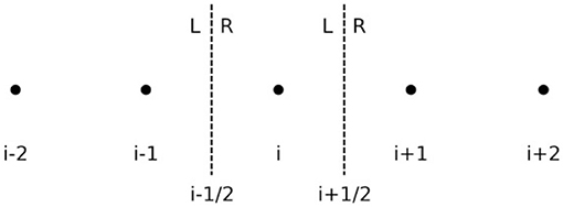
Figure 2. The computational uniform grid x_i. The left (L) and right (R) states reconstructed at the interfaces x_i±1/2 are required to calculate the numerical flux F_i±1/2.

Higher-order schemes are relatively easy to achieve with the finite-difference approach, providing an efficient approach to high-order shock-capturing methods (Shu and Osher, 1988). However, high-order finite-difference numerical schemes applied to the magneto-hydrodynamics (MHD) equations have not been as robust as those based on finite-volume. Nowadays that is not a great inconvenient, and the possibility to achieve high order accuracy is leading to more efforts on implementing these methods on computational MHD codes (Radice et al., 2014; Bernuzzi and Dietrich, 2016). Although the derivation is different, the conservative scheme given by Equation (28) is still valid, where now Ū means just U_i, the value of the field in the grid point. Again, the problem is reduced to compute a suitable numerical flux at the interfaces such that solution is essentially non-oscillatory and preserves, or at least bounds, the Total Variation. The procedure starts by performing a Lax-Friedrichs splitting, where it is introduced the following combination of fluxes and fields $F_i^{\pm }=1/2(F_i\pm \lambda U_i)$, being λ the maximum eigenvalue in the neighborhood of the point. These combinations are interpolated at the interfaces by using a monotonic reconstruction, like the high-order ones discussed before. The flux at the left of the interface $F_{i+1/2}^L$ is reconstructed using the values {F⁺}, while that the flux at the right $F_{i+1/2}^R$ is reconstructed using the values {F⁻}. The final numerical-flux is obtained just as $F_{i+1/2}=F_{i+1/2}^R+F_{i+1/2}^L$. At the lowest order reconstruction, $F_{i+1/2}^L=F_i^{+}$ and $F_{i+1/2}^R=F_{i+1}^{-}$, so that the final numerical-flux reduces to the popular and robust Local-Lax-Friedrichs flux (LeVeque, 1990).

Finally, notice that efforts considering other techniques to solve self-gravitation neutron stars, like the discontinuous Galerkin methods (Hébert et al., 2018), are underway and might be an interesting option in the near future.

Author Contributions

The author confirms being the sole contributor of this work and has approved it for publication.

Funding

I acknowledge support from the Spanish Ministry of Economy and Competitiveness grant AYA2016-80289-P (AEI/FEDER, UE).

Conflict of Interest

The author declares that the research was conducted in the absence of any commercial or financial relationships that could be construed as a potential conflict of interest.

Acknowledgments

It is my pleasure to thank Carles Bona, Miguel Bezares, Luis Lehner, and Joan Massó for their critical reading and helpful comments on the manuscript.

References

Abbott, B. P., Abbott, R., Abbott, T. D., Abraham, S., Acernese, F., Ackley, K., et al. (2019). GWTC-1: a gravitational-wave transient catalog of compact binary mergers observed by LIGO and Virgo during the first and second observing runs. Phys. Rev. X 9:031040. doi: 10.1103/PhysRevX.9.031040

CrossRef Full Text | Google Scholar

Abramovici, A., Althouse, W. E., Drever, R. W. P., Gürsel, Y., Kawamura, S., Raab, F. J., et al. (1992). Ligo: The laser interferometer gravitational-wave observatory. Science 256, 325–333. doi: 10.1126/science.256.5055.325

PubMed Abstract | CrossRef Full Text | Google Scholar

Alcubierre, M. (2008). Introduction to 3+1 Numerical Relativity, OUP Oxford. doi: 10.1093/acprof:oso/9780199205677.001.0001

CrossRef Full Text | Google Scholar

Alcubierre, M., Brügmann, B., Diener, P., Koppitz, M., Pollney, D., Seidel, E., et al. (2003). Gauge conditions for long-term numerical black hole evolutions without excision. Phys. Rev. D 67:084023. doi: 10.1103/PhysRevD.67.084023

CrossRef Full Text | Google Scholar

Alic, D., Bona-Casas, C., Bona, C., Rezzolla, L., and Palenzuela, C. (2012). Conformal and covariant formulation of the Z4 system with constraint-violation damping. Phys. Rev. D 85:064040. doi: 10.1103/PhysRevD.85.064040

CrossRef Full Text | Google Scholar

Anderson, M., Hirschmann, E. W., Lehner, L., Liebling, S. L., Motl, P. M., Neilsen, D., et al. (2008). Simulating binary neutron stars: dynamics and gravitational waves. Phys. Rev. D 77:024006. doi: 10.1103/PhysRevD.77.024006

PubMed Abstract | CrossRef Full Text | Google Scholar

Baiotti, L., Giacomazzo, B., and Rezzolla, L. (2008). Accurate evolutions of inspiralling neutron-star binaries: Prompt and delayed collapse to a black hole. Phys. Rev. D 78:084033. doi: 10.1103/PhysRevD.78.084033

CrossRef Full Text | Google Scholar

Baker, J. G., Centrella, J., Choi, D.-I., Koppitz, M., and van Meter, J. (2006a). Binary black hole merger dynamics and waveforms. Phys. Rev. D 73:104002. doi: 10.1103/PhysRevD.73.104002

CrossRef Full Text | Google Scholar

Baker, J. G., Centrella, J., Choi, D.-I., Koppitz, M., and van Meter, J. (2006b). Gravitational-wave extraction from an inspiraling configuration of merging black holes. Phys. Rev. Lett. 96:111102. doi: 10.1103/PhysRevLett.96.111102

PubMed Abstract | CrossRef Full Text | Google Scholar

Baumgarte, T. W., and Shapiro, S. L. (1999). Numerical integration of Einstein's field equations. Phys. Rev. D 59:024007. doi: 10.1103/PhysRevD.59.024007

CrossRef Full Text | Google Scholar

Baumgarte, T. W., and Shapiro, S. L. (2010). Numerical Relativity: Solving Einstein's Equations on the Computer (Cambridge: Baumgarte and Shapiro). doi: 10.1017/CBO9781139193344

CrossRef Full Text | Google Scholar

Bernuzzi, S., and Dietrich, T. (2016). Gravitational waveforms from binary neutron star mergers with high-order weighted-essentially-nonoscillatory schemes in numerical relativity. Phys. Rev. D 94:064062. doi: 10.1103/PhysRevD.94.064062

CrossRef Full Text | Google Scholar

Bernuzzi, S., and Hilditch, D. (2010). Constraint violation in free evolution schemes: comparing the BSSNOK formulation with a conformal decomposition of the Z4 formulation. Phys. Rev. D 81:084003. doi: 10.1103/PhysRevD.81.084003

CrossRef Full Text | Google Scholar

Bezares, M., Palenzuela, C., and Bona, C. (2017). Final fate of compact boson star mergers. Phys. Rev. D 95:124005. doi: 10.1103/PhysRevD.95.124005

CrossRef Full Text | Google Scholar

Blanchet, L. (2014). Gravitational radiation from post-newtonian sources and inspiralling compact binaries. Living Rev. Relativ. 17:2. doi: 10.12942/lrr-2014-2

PubMed Abstract | CrossRef Full Text | Google Scholar

Bona, C., Bona-Casas, C., and Palenzuela, C. (2010). Action principle for numerical-relativity evolution systems. Phys. Rev. D 82:124010. doi: 10.1103/PhysRevD.82.124010

CrossRef Full Text | Google Scholar

Bona, C., Ledvinka, T., Palenzuela, C., and Žáček, M. (2003). General-covariant evolution formalism for numerical relativity. Phys. Rev. D 67:104005. doi: 10.1103/PhysRevD.67.104005

CrossRef Full Text | Google Scholar

Bona, C., Ledvinka, T., Palenzuela, C., and Žáček, M. (2004). Symmetry-breaking mechanism for the Z4 general-covariant evolution system. Phys. Rev. D 69:064036. doi: 10.1103/PhysRevD.69.064036

CrossRef Full Text | Google Scholar

Bona, C., Massó, J., Seidel, E., and Stela, J. (1995). New formalism for numerical relativity. Phys. Rev. Lett. 75, 600–603. doi: 10.1103/PhysRevLett.75.600

PubMed Abstract | CrossRef Full Text | Google Scholar

Bona, C., and Palenzuela, C. (2004). Dynamical shift conditions for the Z4 and BSSN formalisms. Phys. Rev. D 69:104003. doi: 10.1103/PhysRevD.69.104003

CrossRef Full Text | Google Scholar

Bona, C., Palenzuela-Luque, C., and Bona-Casas, C. (2009). Elements of Numerical Relativity and Relativistic Hydrodynamics, Vol. 783. Berlin; Heidelberg: Springer-Verlag. doi: 10.1007/978-3-642-01164-1

CrossRef Full Text | Google Scholar

Brodbeck, O., Frittelli, S., Hübner, P., and Reula, O. A. (1999). Einstein's equations with asymptotically stable constraint propagation. J. Math. Phys. 40, 909–923. doi: 10.1063/1.532694

CrossRef Full Text | Google Scholar

Brügmann, B., González, J. A., Hannam, M., Husa, S., Sperhake, U., and Tichy, W. (2008). Calibration of moving puncture simulations. Phys. Rev. D 77:024027. doi: 10.1103/PhysRevD.77.024027

PubMed Abstract | CrossRef Full Text | Google Scholar

Calabrese, G., Lehner, L., Reula, O., Sarbach, O., and Tiglio, M. (2004). Summation by parts and dissipation for domains with excised regions. Class. Quant. Grav. 21, 5735–5757. doi: 10.1088/0264-9381/21/24/004

CrossRef Full Text | Google Scholar

Campanelli, M., Lousto, C. O., Marronetti, P., and Zlochower, Y. (2006a). Accurate evolutions of orbiting black-hole binaries without excision. Phys. Rev. Lett. 96:111101. doi: 10.1103/PhysRevLett.96.111101

PubMed Abstract | CrossRef Full Text | Google Scholar

Campanelli, M., Lousto, C. O., and Zlochower, Y. (2006b). Last orbit of binary black holes. Phys. Rev. D 73:061501. doi: 10.1103/PhysRevD.73.061501

CrossRef Full Text | Google Scholar

Caron, B., Dominjon, A., Drezen, C., Flaminio, R., Grave, X., Marion, F., et al. (1997). The Virgo interferometer. Class. Quant. Grav. 14, 1461–1469.

Google Scholar

Font, J. A., Miller, M., Suen, W.-M., and Tobias, M. (2000). Three-dimensional numerical general relativistic hydrodynamics: formulations, methods, and code tests. Phys. Rev. D 61:044011. doi: 10.1103/PhysRevD.61.044011

CrossRef Full Text | Google Scholar

Gourgoulhon, E. (2007). 3+1 Formalism in General Relativity. Lecture Notes in Physics, Vol. 846. Berlin; Heidelberg: Springer-Verlag.

Google Scholar

Gundlach, C., and Martín-García, J. M. (2006). Well-posedness of formulations of the Einstein equations with dynamical lapse and shift conditions. Phys. Rev. D 74:024016. doi: 10.1103/PhysRevD.74.024016

CrossRef Full Text | Google Scholar

Gundlach, C., Martin-Garcia, J. M., Calabrese, G., and Hinder, I. (2005). Constraint damping in the Z4 formulation and harmonic gauge. Class. Quant. Grav. 22, 3767–3774. doi: 10.1088/0264-9381/22/17/025

CrossRef Full Text | Google Scholar

Gustafsson, B., Kreiss, H.-O., and Oliger, J. (1995). Time-Dependent Problems and Difference Methods, 2nd Edn (Wiley).

Google Scholar

Hébert, F., Kidder, L. E., and Teukolsky, S. A. (2018). General-relativistic neutron star evolutions with the discontinuous Galerkin method. Phys. Rev. D 98:044041. doi: 10.1103/PhysRevD.98.044041

CrossRef Full Text | Google Scholar

Hulse, R. A., and Taylor, J. H. (1975). Discovery of a pulsar in a binary system. Astrophys. J. Lett. 195, L51–L53. doi: 10.1086/181708

CrossRef Full Text | Google Scholar

Jiang, G.-S., and Shu, C.-W. (1996). Efficient implementation of weighted eno schemes. J. Comput. Phys. 126, 202–228. doi: 10.1006/jcph.1996.0130

CrossRef Full Text | Google Scholar

Kreiss, H., and Oliger, J. (1973). Methods for the Approximate Solution of Time Dependent Problems. WMO-ICSU; Joint Organizing Committee.

Google Scholar

Lax, P. D., and Richtmyer, R. D. (1956). Survey of the stability of linear finite difference equations. Commun. Pure Appl. Math. 9, 267–293. doi: 10.1002/cpa.3160090206

CrossRef Full Text | Google Scholar

Lehner, L. (2001). TOPICAL REVIEW: numerical relativity: a review. Class. Quant. Grav. 18, R25–R86. doi: 10.1088/0264-9381/18/17/202

CrossRef Full Text | Google Scholar

LeVeque, R. J. (1990). Numerical Methods for Linear Equations. Basel: Birkhäuser Basel. doi: 10.1007/978-3-0348-5116-9_10

CrossRef Full Text | Google Scholar

Lindblom, L., and Scheel, M. A. (2002). Energy norms and the stability of the Einstein evolution equations. Phys. Rev. D 66:084014. doi: 10.1103/PhysRevD.66.084014

CrossRef Full Text | Google Scholar

Lindblom, L., Scheel, M. A., Kidder, L. E., Owen, R., and Rinne, O. (2006). A new generalized harmonic evolution system. Class. Quant. Grav. 23, S447–S462. doi: 10.1088/0264-9381/23/16/S09

CrossRef Full Text | Google Scholar

Liu, Y. T., Shapiro, S. L., Etienne, Z. B., and Taniguchi, K. (2008). General relativistic simulations of magnetized binary neutron star mergers. Phys. Rev. D 78:024012. doi: 10.1103/PhysRevD.78.024012

CrossRef Full Text | Google Scholar

Misner, C. W., Thorne, K. S., and Wheeler, J. A. (1973). Gravitation, 2nd Edn. San Francisco, CA:W H Freeman and Company.

Google Scholar

Mösta, P., Mundim, B. C., Faber, J. A., Haas, R., Noble, S. C., Bode, T., et al. (2014). GRHydro: a new open-source general-relativistic magnetohydrodynamics code for the Einstein toolkit. Class. Quant. Grav. 31:015005. doi: 10.1088/0264-9381/31/1/015005

CrossRef Full Text | Google Scholar

Palenzuela, C., Olabarrieta, I., Lehner, L., and Liebling, S. L. (2007). Head-on collisions of boson stars. Phys. Rev. D 75:064005. doi: 10.1103/PhysRevD.75.064005

CrossRef Full Text | Google Scholar

Pretorius, F. (2005a). Evolution of binary black-hole spacetimes. Phys. Rev. Lett. 95:121101. doi: 10.1103/PhysRevLett.95.121101

PubMed Abstract | CrossRef Full Text | Google Scholar

Pretorius, F. (2005b). Numerical relativity using a generalized harmonic decomposition. Class. Quant. Grav. 22, 425–451. doi: 10.1088/0264-9381/22/2/014

CrossRef Full Text | Google Scholar

Pretorius, F. (2006). Simulation of binary black hole spacetimes with a harmonic evolution scheme. Class. Quant. Grav. 23, S529–S552. doi: 10.1088/0264-9381/23/16/S13

CrossRef Full Text | Google Scholar

Radice, D., Rezzolla, L., and Galeazzi, F. (2014). High-order fully general-relativistic hydrodynamics: new approaches and tests. Class. Quant. Grav. 31:075012. doi: 10.1088/0264-9381/31/7/075012

CrossRef Full Text | Google Scholar

Sarbach, O., Calabrese, G., Pullin, J., and Tiglio, M. (2002). Hyperbolicity of the Baumgarte-Shapiro-Shibata-Nakamura system of Einstein evolution equations. Phys. Rev. D 66:064002. doi: 10.1103/PhysRevD.66.064002

CrossRef Full Text | Google Scholar

Schiesser, W. E. (1991). The Numerical Method of Lines: Integration of Partial Differential Equations. Academic Press.

Google Scholar

Shibata, M. (2015). Numerical Relativity. World Scientific Publishing Co., Inc. doi: 10.1142/9692

CrossRef Full Text | Google Scholar

Shibata, M., and Nakamura, T. (1995). Evolution of three-dimensional gravitational waves: Harmonic slicing case. Phys. Rev. D 52, 5428–5444. doi: 10.1103/PhysRevD.52.5428

PubMed Abstract | CrossRef Full Text | Google Scholar

Shibata, M., and Uryū, K. (2002). Gravitational waves from merger of binary neutron stars in fully general relativistic simulation. Prog. Theor. Phys. 107, 265–303. doi: 10.1143/PTP.107.265

CrossRef Full Text | Google Scholar

Shibata, M., and Uryū, K. ō. (2000). Simulation of merging binary neutron stars in full general relativity: Γ=2 case. Phys. Rev. D 61:064001. doi: 10.1103/PhysRevD.61.064001

CrossRef Full Text | Google Scholar

Shu, C.-W. (1998). “Essentially non-oscillatory and weighted essentially non-oscillatory schemes for hyperbolic conservation laws,” in Advanced Numerical Approximation of Nonlinear Hyperbolic Equations, ed Q. Alfio (Berlin; Heidelberg: Springer), 325–432. doi: 10.1007/BFb0096355

CrossRef Full Text | Google Scholar

Shu, C.-W., and Osher, S. (1988). Efficient implementation of essentially non-oscillatory shock-capturing schemes. J. Comput. Phys. 77, 439–471. doi: 10.1016/0021-9991(88)90177-5

CrossRef Full Text | Google Scholar

Smarr, L., and York, J. W. Jr. (1978). Kinematical conditions in the construction of spacetime. Phys. Rev. D 17, 2529–2551. doi: 10.1103/PhysRevD.17.2529

CrossRef Full Text | Google Scholar

Sperhake, U. (2007). Binary black-hole evolutions of excision and puncture data. Phys. Rev. D 76:104015. doi: 10.1103/PhysRevD.76.104015

CrossRef Full Text | Google Scholar

Suresh, A., and Huynh, H. (1997). Accurate monotonicity-preserving schemes with Runge-Kutta time stepping. J. Comput. Phys. 136, 83–99. doi: 10.1006/jcph.1997.5745

CrossRef Full Text | Google Scholar

Szilágyi, B., Lindblom, L., and Scheel, M. A. (2009). Simulations of binary black hole mergers using spectral methods. Phys. Rev. D 80:124010. doi: 10.1103/PhysRevD.80.124010

CrossRef Full Text | Google Scholar

van Meter, J. R., Baker, J. G., Koppitz, M., and Choi, D.-I. (2006). How to move a black hole without excision: Gauge conditions for the numerical evolution of a moving puncture. Phys. Rev. D 73:124011. doi: 10.1103/PhysRevD.73.124011

CrossRef Full Text | Google Scholar

Will, C. M. (2014). The confrontation between general relativity and experiment. Living Rev. Relat. 17:4. doi: 10.12942/lrr-2014-4

PubMed Abstract | CrossRef Full Text | Google Scholar

Witten, L. (1962). Gravitation: An Introduction to Current Research (Wiley).

Google Scholar

Yamamoto, T., Shibata, M., and Taniguchi, K. (2008). Simulating coalescing compact binaries by a new code (SACRA). Phys. Rev. D 78:064054. doi: 10.1103/PhysRevD.78.064054

CrossRef Full Text | Google Scholar

York, J. W. (1979). “Kinematics and dynamics of general relativity,” in Sources of Gravitational Radiation, ed L. L. Smarr (Cambridge: Cambridge University Press), 83–126.

Google Scholar