On the Detectability of Large-Scale Flows by Asteroseismology

1. Introduction

Large-scale convective motions fundamentally influence stellar structure and evolution. They redistribute angular momentum and energy in the stellar interior, resulting in the generation of differential rotation and meridional circulation (e.g., Ruediger, 1989). Therefore, large-scale convection also represents one of the key ingredients to stellar dynamos, which create magnetic field and thereby activity cycles in stars (e.g., Miesch, 2005). Many stars feature an extensive outer convection zone, but not much is known about the more detailed organization of convection, in particular concerning dominant cell formations or cell sizes, as well as the corresponding flow velocities, which are related to the energy transport. This lack of knowledge is due to the fact that stellar surfaces are typically not spatially resolved by observations. Here asteroseismology represents a unique opportunity to obtain information from observations even in the absence of spatial resolution.

For the Sun, the most prominent convective feature on the surface are the small-scale granules. Large-scale convection is also believed to operate throughout the solar convection zone. Based on measurements of the Doppler velocity on the solar surface Hathaway et al. (2013) found evidence for giant convection cells, but its internal structure is controversially discussed (Hanasoge et al., 2012; Hanasoge and Sreenivasan, 2014; Greer et al., 2015). For more evolved stars, such as subgiant stars and red giants, modeling suggests that surface convection organizes into larger cells with higher flow velocities (e.g., Trampedach et al., 2013; Tremblay et al., 2013), rendering these stars ideal candidates for the investigation of large-scale convective flows. Imaging the details of large-scale flows on supergiants supports these findings (López Ariste et al., 2018; Montargès et al., 2018). In this work, we will focus on the effect of large-scale flows on the observed asteroseismic signal.

In this article, we describe the influence of large-scale poloidal flow cells on global stellar oscillation modes. Our aim is to determine the signatures of flows in seismic data that could be used to detect or characterize flows from observations. The investigation is carried out by means of forward calculations, where we employ perturbation theory as proposed by Lavely and Ritzwoller (1992). For this, the vector flow field inside the star is decomposed into its poloidal and toroidal components. The poloidal component is used to describe the giant cells as it has all three vector components. The toroidal component has a vanishing radial component, i.e., it describes flows on the surface of a torus, i.e., in our context on a spherical surface. In this framework, the presence of a flow leads to a coupling of the global stellar oscillation modes, which results in frequency shifts and a mixing of the mode eigenfunctions. For the Sun, forward calculations employing this method have already been performed by Roth and Stix (2008), Chatterjee and Antia (2009), and Schad (2013), who studied the axisymmetric meridional flow, and by Roth and Stix (1999), Roth et al. (2002), and Chatterjee and Antia (2009), examining certain non-axisymmetric cell formations. In this contribution we explore mode coupling in an asteroseismic context. For this purpose we examine the effects of flows on low-degree modes and estimate potentially observable signatures. We put particular focus on axisymmetric and non-axisymmetric poloidal cell formations, which, in the solar context, are also referred to as merdidional flows and giant cells, resp. The calculations presented here cover the non-rotating and the rotating case. In an exemplary application we derive these signatures for a subgiant stellar model.

2. Methods

We calculate the effect of convective flows on oscillation modes of stars by employing quasi-degenerate perturbation theory applied to stars and their oscillations, as presented in Lavely and Ritzwoller (1992). Complementary, the results from the quasi-degenerate calculations are approximated by perturbation expansions, where we utilize an ansatz presented in Schad (2011).

2.1. Equilibrium Model

Starting point of our calculations is a 1D static and non-rotating equilibrium stellar model with oscillation modes ξ_k and corresponding frequencies ω_k. Here k = (n, l, m) is a multiindex, which consists of three indices that characterize each oscillation mode. By considering small perturbations of the equilibrium model due to a displacement ξ of a parcel of gas, it can be shown (e.g., Aerts et al., 2010) that the oscillation modes ξ_k of the model are governed by the momentum equation

$\begin{array}{ll}{\omega }_k^2{\xi }_k={{L}}_0{\xi }_k,& (1)\end{array}$

where the linear operator ${{L}}_0$ is defined by

$\begin{array}{ll}{{L}}_0\xi =\frac{1}{{\rho }_0}\nabla p^{\prime }-g^{\prime }-\frac{{\rho }^{\prime }}{{\rho }_0}{g}_0.& (2)\end{array}$

Here p′, ρ′, and g′ denote Eulerian perturbations of pressure, density, and gravitational acceleration, respectively. The subscript 0 indicates equilibrium quantities. Equation (1) represents an eigenvalue problem for ${{L}}_0$, which is solved by eigenfunctions

$\begin{array}{ll}\xi (r,\theta ,\varphi )={\xi }^r(r)Y_l^m(\theta ,\varphi )e_r+{\xi }^h(r){\nabla }_h{Y}_l^m(\theta ,\varphi ),& (3)\end{array}$

where $Y_l^m$ is a spherical harmonic of harmonic degree l and azimuthal order |m| ≤ l, ξ^r, and ξ^h are radial eigenfunctions of the radial and horizontal component of ξ, e_r denotes the unit vector in radial direction, and the horizontal gradient ∇_h is given by

$\begin{array}{ll}{\nabla }_{\text{h}}=\frac{\partial }{\partial \theta }{e}_{\theta }+\frac{1}{\text{sin }\theta }\frac{\partial }{\partial \varphi }{e}_{\varphi }.& (4)\end{array}$

We normalize the eigenfunctions such that

$\begin{array}{ll}{\displaystyle {\int }_0^R}{\rho }_0\left(|{\xi }^r{|}^2+l(l+1)|{\xi }^h{|}^2\right)r^2\text{d}r=1,& (5)\end{array}$

with R as stellar radius. For the equilibrium model, which we assume to be spherically symmetric, modes of the same radial order n and harmonic degree l form multiplets (n, l) that consist of modes with different azimuthal orders m but identical frequencies ω_nl, i.e., the frequencies of the modes are degenerate in m.

2.2. Perturbation by a Global Velocity Field

A flow inside a star, such as rotation or convection, represents a velocity field that can be treated as a perturbation of the equilibrium model, provided the flow velocity is small compared to the speed of sound. The velocity field moves the stellar plasma and therefore advects waves traveling in this plasma. Hence, the oscillation modes have to fulfill a perturbed momentum equation

$\begin{array}{ll}{\omega }_k^2{\xi }_k={{L}}_0{\xi }_k+{{L}}_1{\xi }_k,& (6)\end{array}$

where ${{L}}_1$ represents the advective effect of a velocity field u, given by

$\begin{array}{ll}{{L}}_1{\xi }_k=-2i\omega (u·\nabla ){\xi }_k-2i\omega \Omega \times {\xi }_k.& (7)\end{array}$

The second term on the right hand side of Equation (7) accounts for the effect of the Coriolis force and only needs to be taken into account when working in a rotating (with constant angular velocity Ω) reference frame.

Following the approach of Lavely and Ritzwoller (1992), we utilize a spherical harmonic decomposition of the velocity field u, consisting of a poloidal part P and a toroidal part T:

$\begin{array}{ll}u(r)={\displaystyle \sum _{s=0}^{\infty }}{\displaystyle \sum _{t=-s}^s}{P}_s^t(r,\theta ,\varphi )+T_s^t(r,\theta ,\varphi ),& (8)\end{array}$

with

$\begin{array}{ll}{P}_s^t(r,\theta ,\varphi )=u_s^t(r)Y_s^t(\theta ,\varphi )e_r+v_s^t(r){\nabla }_h{Y}_s^t(\theta ,\varphi ),& (9)\end{array}$

$\begin{array}{ll}{T}_s^t(r,\theta ,\varphi )=-w_s^t(r)e_r\times {\nabla }_h{Y}_s^t(\theta ,\varphi ).& (10)\end{array}$

The components of expansion (8) are characterized by the radius dependent expansion coefficients $u_s^t(r)$, $v_s^t(r)$ and $w_s^t(r)$. We only consider flows that are stationary in time and anelastic

$\begin{array}{ll}\nabla ·({\rho }_0\text{u})=0.& (11)\end{array}$

Therefore, the coefficients $u_s^t(r)$ and $v_s^t(r)$ of the poloidal components are not independent but connected by mass conservation

$\begin{array}{ll}\frac{\partial }{\partial r}(r^2{\rho }_0{u}_s^t)={\rho }_{0}rs(s+1)v_s^t.& (12)\end{array}$

The conditions of stationarity and anelasticity are used as an approximation for a flow that varies on time scales longer than the stellar oscillation periods. To construct a real valued velocity field the conditions

$\begin{array}{ll}{u}_s^{-t}={(-1)}^t{u_s^t}^{*},v_s^{-t}={(-1)}^t{v_s^t}^{*},\text{ and }{w}_s^{-t}={(-1)}^t{w_s^t}^{*}& (13)\end{array}$

have to be satisfied by the expansion coefficients (Dahlen and Tromp, 1998), which implies specifically for non-axisymmetric flows (t ≠ 0) that both, the positive and the negative t-component are to be included in expansion (8).

2.3. Quasi-Degenerate Perturbation Theory

In the following, we briefly outline the approach of quasi-degenerate perturbation theory as used in this context. For details we refer to the original description by Lavely and Ritzwoller (1992).

As shown above advection leads to a perturbation of the oscillation equation (6). In first-order perturbation theory the perturbed oscillation eigenfunction is described in terms of the unperturbed eigenfunctions. To calculate the respective expansion coefficients and the perturbed eigenfrequencies, which mirror the perturbing effect of the velocity field on the oscillation modes of a star, a matrix representation of the perturbation has to be constructed. Lavely and Ritzwoller (1992) apply quasi-degenerate perturbation theory, which can be regarded as a local approach, since the perturbation is calculated by considering only a limited range Δω² around the oscillation frequency of interest ω_ref. This is expressed in the quasi-degeneracy condition

$\begin{array}{ll}|{\omega }_k^2-{\omega }_{\text{ref}}^2|<\Delta {\omega }^2.& (14)\end{array}$

Thereby, the choice of the range Δω² defines a subset K of modes contributing to the calculation. The matrix representation of the perturbation within quasi-degenerate perturbation theory is given by a so-called supermatrix Z, the matrix elements of which can be calculated by

$\begin{array}{ll}{Z}_{k^{\prime }k}=H_{k^{\prime }k}+({\omega }_k^2-{\omega }_{\text{ref}}^2){\delta }_{k^{\prime }k},& (15)\end{array}$

where the matrix elements $H_{k^{\prime }k}$ compose the matrix representation of the perturbation operator ${{L}}_1$, which is called the general matrix H:

$\begin{array}{ll}{H}_{k^{\prime }k}={\displaystyle {\int }_V}{\rho }_0{\xi }_{k^{\prime }}^{*}·({{L}}_1){\xi }_k\text{d}V.& (16)\end{array}$

These general matrix elements can be calculated by (cf. Lavely and Ritzwoller, 1992)

$\begin{array}{ll}{H}_{k^{\prime }k}=B_{k^{\prime }k}+C_{k^{\prime }k}.& (17)\end{array}$

The Coriolis contribution $B_{k^{\prime }k}$ is given by

$\begin{array}{ll}{B}_{k^{\prime }k}=-{\delta }_{m^{\prime }m}{\delta }_{l^{\prime }l}2{\omega }_{\text{ref}}m\Omega {\displaystyle {\int }_0^{R_{\odot }}}{\rho }_0\left({\xi }^r{{\xi }^h}^{\prime }+{{\xi }^r}^{\prime }{\xi }^h+{\xi }^h{{\xi }^h}^{\prime }\right)r^2\text{d}r,& (18)\end{array}$

where Ω = |Ω| is the angular velocity of the frame of reference in which the calculations are performed. The contribution from advection is

$\begin{array}{l}{C}_{k^{\prime }k}=-8\pi {\omega }_{\text{ref}}{\gamma }_{l^{\prime }}{\gamma }_l{(-1)}^{m^{\prime }}{\displaystyle \sum _{s=0}^{\infty }}{\displaystyle \sum _{t=-s}^s}{\gamma }_s\left(\begin{array}{ccc}s& l& l^{\prime }\\ t& m& -m^{\prime }\end{array}\right)\\ \begin{array}{l}·{\displaystyle {\int }_0^{R_{\odot }}}{\rho }_0\left[i{u}_s^t(r)R_s(r)+i{v}_s^t(r)H_s(r)+w_s^t(r)T_s(r)\right]r^2\text{d}r,\end{array}& (19)\end{array}$

where ${\gamma }_x=\sqrt{(2x+1)/(4\pi )}$ with x = s, l, l′. For the expressions of the kernels R_s(r), H_s(r), and T_s(r), see Appendix 1. The symbol

$\begin{array}{ll}\left(\begin{array}{ccc}s& l& l^{\prime }\\ t& m& -m^{\prime }\end{array}\right),& (20)\end{array}$

occurring in Equation (19), denotes the Wigner-3j symbol, which expresses an integration over angular components, i.e., spherical harmonics, that appears implicitly in Equation (16). The Wigner-3j symbol determines the coupling of the angular part of two modes via the flow. For a more detailed description of the properties of the Wigner-3j symbol see, e.g., Edmonds (1960) or Lavely and Ritzwoller (1992). Two modes k, k′ couple, if the element $H_{k^{\prime }k}$ of the general matrix is non-zero. Two selection rules of mode coupling result from the Wigner-3j symbols: the harmonic degrees have to fulfill the triangle inequality

$\begin{array}{ll}|s-l|\le l^{\prime },|l-l^{\prime }|\le s,|l^{\prime }-s|\le l,& (21)\end{array}$

and the azimuthal orders have to satisfy

$\begin{array}{ll}t+m-m^{\prime }=0.& (22)\end{array}$

For non-axisymmetric flows (t ≠ 0), which have to be composed of a positive and negative component of azimuthal order ±t, selection rule (Equation 22) leads to sets of coupling modes in which degeneracy occurs, since a mode with azimuthal order m has two direct coupling partners m′ = m ± t from each multiplet fulfilling Equation (21). Generally, the supermatrix for a given reference multiplet (n, l) can be decomposed into several independent, irreducible submatrices, where number and sizes of the submatrices depend on the flow configuration. If two modes of different azimuthal order m from the reference multiplet are part of the same irreducible submatrix, we speak of a degenerate coupling set.

To obtain the new perturbed quantities, i.e., perturbed eigenfunctions and frequencies of oscillation modes, we solve the eigenvalue problem for the supermatrix Z (or equivalently for the irreducible submatrices, which is computationally less demanding)

$\begin{array}{ll}ZA=A\Lambda .& (23)\end{array}$

The matrix Λ contains the eigenvalues ${({\omega }_z^2)}_k$ in its diagonal and the matrix A contains the eigenvectors in its columns, which are composed of expansion coefficients $a_{k^{\prime }}^k$ that form the new eigenfunctions $\tilde{\xi }$ via

$\begin{array}{ll}{\tilde{\xi }}_k={\displaystyle \sum _{k^{\prime }\in K}}{a}_{k^{\prime }}^k{\xi }_{k^{\prime }}.& (24)\end{array}$

From the eigenvalues ${({\omega }_z^2)}_k$, which represent squared frequency corrections, the new frequencies ${\tilde{\omega }}_k$ and consequently the frequency shifts δω_k can be determined. We have

$\begin{array}{ll}{\tilde{\omega }}_k^2={\omega }_{\text{ref}}^2+{({\omega }_z^2)}_k,& (25)\end{array}$

therefore we obtain for the frequency shifts

$\begin{array}{ll}\delta {\omega }_k={\tilde{\omega }}_k-{\omega }_k=\sqrt{{\omega }_{\text{ref}}^2+{({\omega }_z^2)}_k}-{\omega }_{\text{ref}},& (26)\end{array}$

where we have used the fact that ω_k = ω_ref, when calculating the frequency shift for the frequency of interest ω_k.

We refer to the method of obtaining perturbed quantities directly from the solution of the eigenvalue problem of Z as the quasi-degenerate method, or in short the QD method.

2.4. Approximation by Perturbation Expansions

As the computational effort of the eigenvalue calculation of the matrix Z increases with the dimensions of the matrix, Schad (2011) and Roth and Stix (1999) describe an alternative approach for solving the eigenvalue problem in the non-degenerate case: Not all modes k′ contribute to the perturbation of the reference mode k. The coupling of the modes is determined by the Wigner 3j symbols and the kernels, meaning that many matrix elements of Z vanish. Hence, the eigenvalues and eigenvectors of Z can be approximated by perturbation expansions. We make use of their approach and briefly summarize this procedure, which we refer to as the PE method.

To shorten the expressions we utilize the abstract bra-ket notation and therefore denote eigenstates as |k〉. The eigenfunctions ξ_k introduced earlier are the corresponding representation in position space of the eigenstates |k〉.

Following Schad (2011), the perturbation expansion for the eigenvalues of Z up to second order is of the form

$\begin{array}{ll}{({\omega }_z^2)}_k\approx E_k^{(0)}+E_k^{(1)}+E_k^{(2)},& (27)\end{array}$

where the E_k denote eigenvalue corrections and the zeroth order correction is given by $E_k^{(0)}={\omega }_k^2-{\omega }_{\text{ref}}^2$. Since we generally work with ω_k = ω_ref, this term is equal to zero. For the first and second order corrections, one has to distinguish between three different cases: non-degenerate, degenerate and second order degenerate.

Due to the triangle inequality (Equation 21) and the dependency of the kernels R_s, and H_s on l, l′ and s the non-degenerate case occurs e.g., for any poloidal axisymmetric flow (t = 0), but for non-axisymmetric poloidal flows only in case of certain combinations of flow configuration and modes, namely

$\begin{array}{ll}\Vert m|-2t|>l\text{ for }s\text{ odd},& (28)\end{array}$

$\begin{array}{ll}\Vert m|-t|>l\text{ for }s\text{ even}.& (29)\end{array}$

In the non-degenerate case the first and second order eigenvalue corrections are given by (compare with Schad, 2011, Equations 30 and 31)

$\begin{array}{ll}{E}_k^{(1)}=H_{kk}{E}_k^{(2)}={\displaystyle \sum _{j\ne k}}\frac{|H_{jk}{|}^2}{{\omega }_{\text{ref}}^2-{\omega }_j^2}.& (30)\end{array}$

Extending the approach just described to the degenerate case, let D ⊂ K be the set of degenerate oscillation modes. If the degeneracy is lifted in first order (e.g., if a non-axisymmetric poloidal flow is combined with rotation) we obtain

$\begin{array}{ll}{E}_k^{(1)}=H_{kk}^{Dd},E_k^{(2)}={\displaystyle \sum _{j\notin D}}\frac{|{\displaystyle {\sum }_{n\in D}}{c}_n^k{H}_{jn}{|}^2}{{\omega }_{\text{ref}}^2-{\omega }_j^2},& (31)\end{array}$

where $H_{kk}^{Dd}$ denote the eigenvalues of the matrix H^D, which is the subsection of the matrix H spanned by degenerate modes n ∈ D. The coefficients $c_n^k$, which occur in the second order eigenvalue correction are determined by the components of the eigenvectors |k〉_D of H^D with

$\begin{array}{ll}{|k\rangle }_D={\displaystyle \sum _{n\in D}{c}_n^k}|n^0\rangle ,& (32)\end{array}$

where the superscript 0 denotes unperturbed states.

If degeneracy is present, but the first order correction is zero (e.g., non-axisymmetric flows, no rotation) the degeneracy is not lifted in first order and degeneracy of second order occurs. One then has

$\begin{array}{ll}{E}_k^{(1)}=0,E_k^{(2)}=W_{kk}^{Dd},& (33)\end{array}$

where $W_{kk}^{Dd}$ denote the eigenvalues of a perturbation matrix of second order W^D (cf., e.g., Schiff, 1968).

The perturbation expansion for the eigenvectors of Z up to first order is of the form

$\begin{array}{ll}{|k\rangle }_z\approx {\displaystyle \sum _{n\in D}{c}_n^k}|n^0\rangle +{\displaystyle \sum _{j\notin D}|j^0\rangle }\frac{{\displaystyle {\sum }_{n\in D}{c}_n^k}\langle j^0|H|n^0\rangle }{{\omega }_n^2-{\omega }_j^2}.& (34)\end{array}$

In the non-degenerate case, the coefficients $c_n^k$ are given by Kronecker delta functions $c_n^k={\delta }_{nk}$. In the degenerate cases the coefficients $c_n^k$ are determined either from the eigenvectors of the matrix H^D or W^D respectively, depending on whether the degeneracy is lifted in first or in second order.

3. Models

3.1. Stellar Models

For our exemplary calculations we focus on a subgiant star. The model for this star was calculated with the MESA stellar evolution code (Paxton, 2011), and has a mass of 1.25M_⊙. We started with an initial metallicity of Z = 0.02 and an initial He abundance of Y = 0.28 and evolved the star for 4.6 Gyr to a stage where a substantial helium core has developed, which is not ignited yet but surrounded by a hydrogen burning shell. At this stage, the convection zone extends roughly through the outer 29% of the stellar radius and is quickly expanding with age. The convective regions were determined by the Schwarzschild criterion and—for simplicity—no overshoot was added. Table 1 summarizes the parameters of the stellar model. The unperturbed oscillation modes of the subgiant model were computed with ADIPLS (Christensen-Dalsgaard, 2008).

TABLE 1

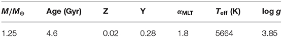
Table 1. Subgiant model parameters.

We note that in contrast to a main-sequence star such as the Sun, which features pure p- and g-modes, a subgiant star harbors mixed modes, which however can also be mainly of p-type or of g-type. To distinguish between p-type and g-type mixed modes, we calculate the mode inertia (e.g., Dupret et al., 2009) in the convection zone

$\begin{array}{ll}{\epsilon }_{\text{cz}}={\displaystyle {\int }_{r_{\text{min}}}^R}\left(|{\xi }^r(r){|}^2+l(l+1){|{\xi }^h(r)|}^2\right){\rho }_0{r}^2\text{d}r,& (35)\end{array}$

with r_min being the radius of the bottom of the convection zone. Since the eigenfunctions are normalized such that the total mode inertia is equal to unity (cf. Equation 5), Equation (35) also represents the relative inertia in the convection zone. Figure 1 displays ${\epsilon }_{\text{cz}}$ for the modes of the subgiant up to harmonic degree l = 7, including all radial orders n in the frequency range from 400 to 900 μHz. For the l = 0 modes, which are pure p modes, the inertia in the convection zone amounts to about 65% of the total inertia. For l = 1 the modes start to separate in their inertia values dropping to lower values when becoming increasingly mixed. The modes have still a significant inertia in the convection zone and can be affected by the flow. For higher l, the modes settle to form two clusters, one with high (p-type modes) and one with low inertia (g-type modes) in the convection zone, where the low inertia modes will have little to no sensitivity to convective poloidal flow cells.

FIGURE 1

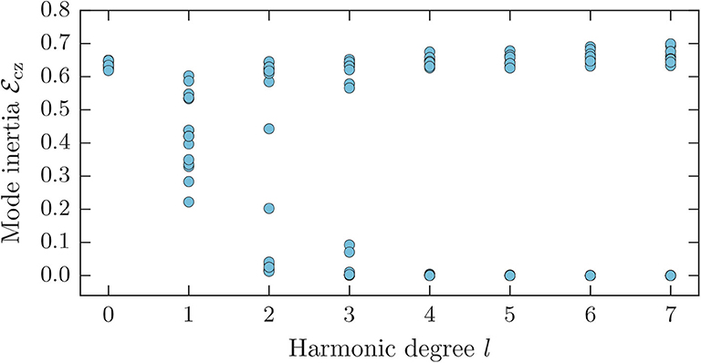
Figure 1. Mode inertia in the convection zone of the subgiant for modes of harmonic degree l = 0, …, 7 and all radial orders n occurring in the frequency range 400 − 900 μHz.

3.2. Poloidal Flow Model

To describe the fundamental effect of a flow on oscillations it is instructive to consider different harmonic components of the harmonic expansion (8) of the flow individually. The poloidal flow fields we use in our calculations will therefore read

$\begin{array}{ll}{u}_s^t(r,\theta ,\varphi )={\displaystyle \sum _{t^{\prime }=\pm t}}{u}_s^{t^{\prime }}(r)Y_s^{t^{\prime }}(\theta ,\varphi )e_r+v_s^{t^{\prime }}(r){\nabla }_h{Y}_s^{t^{\prime }}(\theta ,\varphi ),& (36)\end{array}$

where as mentioned above, both, the positive and negative values of t appear to guarantee a real-valued flow field. The expansion coefficients $u_s^t(r)$ and $v_s^t(r)$ of the radial and horizontal component of the vector field represent depth dependent flow strengths. Since the coefficients are connected by Equation (12), only one of them has to be prescribed. We choose $u_s^t(r)$ to have a sinusoidal shape, analogously to Roth and Stix (2008)

$\begin{array}{ll}{u}_s^t=u_a\text{ sin }\left(\pi \frac{r-r_{\text{min}}}{r_{\text{max}}-r_{\text{min}}}\right),& (37)\end{array}$

where r_min and r_max denote the inner and outer boundary of the convection zone, respectively. At those boundaries this simple model ensures that the radial flow component vanishes. For the amplitude u_a = 150 m/s we use for our purposes of deriving a first estimate of the expected effect the velocities obtained from the mixing-length theory (MLT), which is used to treat convection in the computation of the stellar model (Böhm-Vitense, 1958). Figure 2 shows the flow profile $u_s^t(r)$ entering our calculations, together with the resulting $v_s^t(r)$ for an example harmonic degree s = 9. Additionally, the velocity profile obtained from the MLT is displayed for comparison.

FIGURE 2

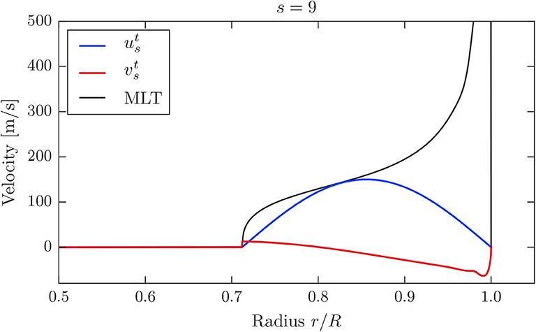
Figure 2. Profiles of the poloidal flow components $u_s^t$ and $v_s^t$ (for s = 9) as a function of stellar radius. The MLT velocity profile of the stellar model is shown for comparison.

3.3. Rotational Flow Model

Rotation can be modeled by a toroidal velocity field (cf. Equation 10). For simplicity we employ here only radial differential rotation and no latitudinal variation of rotation, which can be modeled with a single coefficient $w_1^0(r)$ in expansion (8). We prescribe a rotational configuration where the core of the star, which is separated from the stellar envelope by the hydrogen burning shell, rotates faster than the envelope. This configuration is typical for subgiant stars (cf. e.g., Deheuvels et al., 2014). For the subgiant model employed here, the hydrogen burning shell is located at about r/R ≈ 0.029. Based on the results of Deheuvels et al. (2014), we set the envelope rotation rate to 250 nHz and the core rotation rate to 620 nHz, hence

$\begin{array}{ll}\begin{array}{l}\Omega (r)=\{\begin{array}{ccc}620·2\pi \hfill & \text{for}\hfill & r\le 0.029·R\hfill \\ 250·2\pi \hfill & \text{for}\hfill & r>0.029·R\hfill \end{array}\hfill \end{array}.& (38)\end{array}$

The resulting depth dependent velocity profile $w_1^0(r)$ is then obtained via (cf. Ritzwoller and Lavely, 1991)

$\begin{array}{ll}{w}_1^0(r)=2\sqrt{\frac{\pi }{3}}r\Omega (r).& (39)\end{array}$

In case of a rotating star, we assume that the poloidal flow cells rotate with the envelope angular velocity. Hence, the poloidal flow cells will be stationary in a reference frame co-rotating with the envelope at Ω_sys/(2π) = 250 nHz. Since the method described in section 2 is only valid for stationary flows, the calculations have to be carried out in this co-rotating frame. The results can then be transformed into an inertial frame of reference to model observations carried out from Earth.

4. Results for Purely Poloidal Flows (Non-rotating Star)

When observing stars other than the Sun photometrically, only modes of low degree l ≤ 3 can be detected. Modes of higher degree are subject to canceling effects (cf. e.g., Dziembowski, 1977), since observations, up to now, generally do not resolve the stellar surface. In this section, where a non-rotating star is considered, we present results for dipole (l = 1) modes, since they show, together with the l = 0 modes, the highest amplitudes in stellar oscillation spectra. In section 5, where the more general case of a rotating star is examined, we also present results for exemplary l = 0 and l = 2 modes.

4.1. Frequency Shifts, Non-degenerate Case

In Figure 3 exemplary frequency shifts δν = δω/2π for three different dipole multiplets in a frequency range typical for subgiant stars are presented. For these results a configuration with s = 9 for the poloidal flow cells was used and the azimuthal order t of the flow was varied through all corresponding values |t| = 0, 2, …, 9, for which the reference modes are non-degenerate in the coupling set of modes. The case |t| = 1 is not considered since a degenerate coupling set occurs. From Figure 3, it is evident that the flow causes the originally degenerate triplets consisting of three modes with m = −1, 0, 1 to split up into two components, an m = 0 and an m = ±1 component. This shows that poloidal flows shift modes of opposite azimuthal order ±m equally, provided they are not connected through the perturbation by the flow, i.e., they are part of non-degenerate coupling sets. Figure 3 also shows that the shifts exhibit a distinct pattern depending on t. For each multiplet the two components cross between the flow configurations with t = 5 and t = 6. This behavior is induced by the Wigner-3j symbols entering the general matrix elements (cf. Equation 19). The magnitude of the shifts varies for the different multiplets, but in general the shift is of the order of 10⁻¹ nHz to 1 nHz, which is challenging with today's observational capabilities.

FIGURE 3

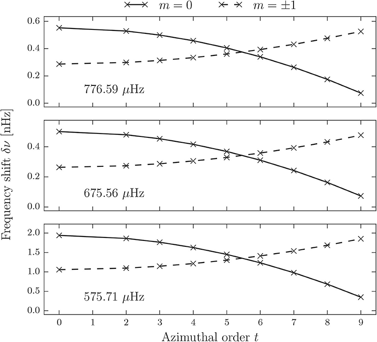
Figure 3. Frequency shifts for three l = 1 multiplets of the subgiant star for a flow configuration with s = 9 and |t| = 0, 2, …, 9. Shifts of the m = 0 mode are connected by a solid line, shifts of the m = +1 and m = −1 modes are of equal value and connected by a dashed line.

To explore the dependence of the frequency shifts on the harmonic degree s of the flow, we calculated the shifts for different values of s for one reference multiplet at 675.6 μHz. In Figure 4, the frequency shifts for various flow degrees s = 3, …, 9 and the corresponding values of t are displayed. For better visibility, shifts for the m = 0 and the m = ±1 component are plotted in separate panels. The magnitude of the shifts fluctuates for different s values, but there is no definite trend with s visible.

FIGURE 4

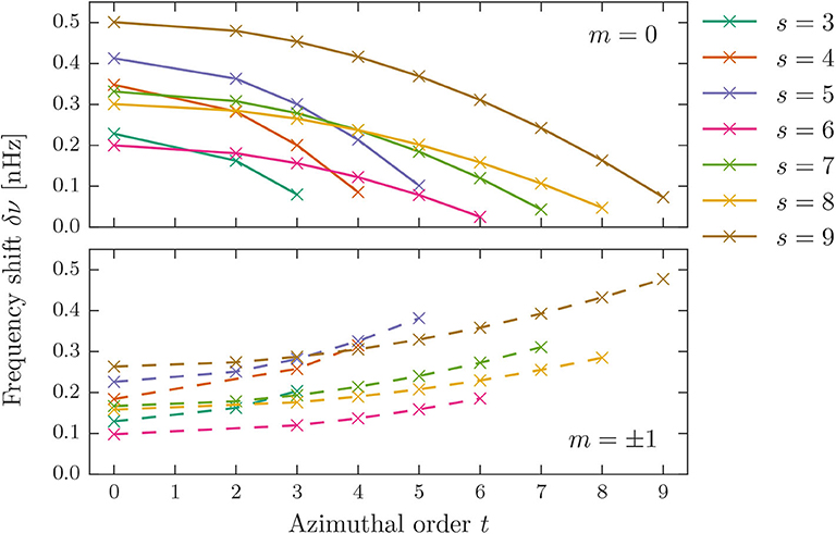
Figure 4. Frequency shifts for different flow degrees s and the corresponding azimuthal orders t for a dipole multiplet at ν = 675.6 μHz. (Top) shifts of the m = 0 component. (Bottom) shifts of the m = ±1 component.

4.2. Frequency Shifts, Degenerate Case

In case of degenerate coupling sets, two or more modes of the reference multiplet are connected by the perturbation. In this case, the modes that experience the frequency shift are generally not oscillation eigenstates inasmuch as they have no well-defined azimuthal order. As an example, the frequency shifts for the dipole multiplet at 675.6 μHz for a flow configuration with s = 5 and t = 1 are displayed in Figure 5. For this flow configuration, degeneracy occurs between the m = 1 and m = −1 oscillation states, since they are part of the same coupling set. The two states that the flow acts on, are here orthogonal linear combinations of the two degenerate states with equal mixing coefficients

$\begin{array}{ll}\text{State }1:\frac{1}{\sqrt{2}}|m=-1\rangle +\frac{1}{\sqrt{2}}|m=+1\rangle & (40)\end{array}$

$\begin{array}{ll}\text{State }2:\frac{1}{\sqrt{2}}|m=-1\rangle -\frac{1}{\sqrt{2}}|m=+1\rangle .& (41)\end{array}$

As is also evident from Figure 5, the frequency shifts of these states are not equal, so the multiplet will split up into three components of different frequency. The magnitude of the shifts is comparable to the non-degenerate cases.

FIGURE 5

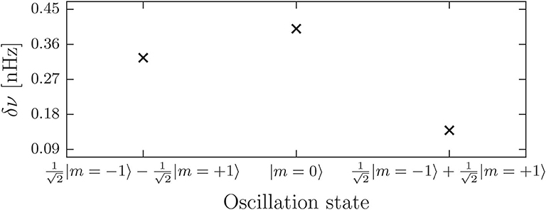
Figure 5. Frequency shifts for the dipole multiplet at ν = 675.6 μHz for a flow configuration with s = 5 and t = 1, for which a degenerate coupling set occurs. The shifts have to be assigned to mixed states instead of oscillation eigenstates.

5. Results for Poloidal Flows in Rotating Stars

When rotation is included in the calculation, the degeneracy of the multiplets is lifted by the effect of rotation in first order. Since the general matrix of rotation is diagonal in the degenerate subspaces of the multiplets, the eigenstates that the perturbation acts on are pure oscillation eigenstates with a well-defined azimuthal order.

As noted in section 3.3, for rotating stars, we carry out the perturbation calculation in a frame of reference co-rotating with the poloidal flow cells, to adhere to the required stationarity of the flow. Therefore we will present the results for frequency shifts in the co-rotating frame (section 5.1). In the frame of a stationary observer, all frequencies would appear shifted by an additional mΩ_sys, which is but of no consequence to the discussion here.

The additional frequency shift, however, is not the only effect that has to be considered when changing from a co-rotating to an inertial system. Taking into account the eigenfunction perturbations, a switch of reference frames will actually lead to a multiperiodic signal for each perturbed mode in the inertial frame, which is discussed in section 5.2.

5.1. Frequency Shifts in the Co-rotating Frame

When poloidal flows occur in combination with rotation, the resulting frequency shifts will be asymmetric for modes of opposite azimuthal order ±m. Therefore we start the discussion of frequency shifts by elaborating on the different origins of asymmetries in section 5.1.1. In the following sections 5.1.2–5.1.4, the effect of the flow on modes of harmonic degree l = 0, 1, 2 is investigated, since these modes typically exhibit observable amplitudes in stellar oscillation spectra. The results are summarized in section 5.1.5.

For the calculations, we adopt for the poloidal flow a cell configuration with s = 8 and the possible corresponding values of t, ranging from meridional (t = 0) to sectoral (t = s) cells. For better visibility of the effects, the amplitude u_a of the velocity profile (Equation 37) of the flow is amplified by a factor of five. The main calculation is performed with the QD method (section 2.3), but the PE method (section 2.4) is used as comparison to distinguish different effects in the results.

5.1.1. Frequency Shift Asymmetries

If the frequency shift for modes of opposite azimuthal order ±m is of equal value, we speak of a symmetric frequency shift. In contrast, if the shift has opposite value for modes of opposite azimuthal order, we speak of an antisymmetric frequency shift. For a poloidal flow combined with rotation, the occurring frequency shifts will be asymmetric for modes of opposite azimuthal order ±m. This is due to the fact that the first order eigenvalue corrections are antisymmetric in m (they are given by the diagonal elements of the general matrix (cf. Equation 31) which originate from rotation) and the second order corrections, which are generated by squared matrix elements of the poloidal flow, are symmetric in m. There are, however, two additional small effects that can lead to asymmetries in the frequency shifts. First, the third order eigenvalue correction can gain a notable magnitude, in particular for a rotational configuration with a faster rotating core, as prescribed here. The third order eigenvalue correction adapted from Sakurai and Napolitano (2011) for a perturbation composed of rotation and a poloidal flow, is given by

$\begin{array}{ll}{E}_k^{(3)}={\displaystyle \sum _{j\notin D}}{\displaystyle \sum _{i\notin D}}\frac{H_{ki}{H}_{ij}{H}_{jk}}{({\omega }_i^2-{\omega }_k^2)({\omega }_j^2-{\omega }_k^2)}-H_{kk}{\displaystyle \sum _{i\notin D}}\frac{|H_{ki}{|}^2}{{({\omega }_i^2-{\omega }_k^2)}^2}.& (42)\end{array}$

The second effect causing an asymmetry originates from the fact, that rotation combined with a poloidal flow leads (in most cases), just as a purely poloidal flow, to degenerate coupling sets. Rotation lifts this degeneracy in first order, but the coupling of modes by the poloidal flow within a degenerate coupling set occurs in second order, which can lead to a notable asymmetry in the frequency shifts for ±m, and a mixing of the eigenvectors of zeroth order, analogously to the results presented for the degenerate case in section 4.2. This type of asymmetry, caused by degenerate coupling, cannot be reproduced by an approximation with a perturbation expansion.

5.1.2. Modes of Degree l = 0

Modes of harmonic degree l = 0 are pure p modes. They do not occur in multiplets, therefore no degeneracy can arise. Additionally l = 0 modes are not affected by rotation. Poloidal flows on the other hand will cause a frequency shift for l = 0 modes. This shift however does not depend on the azimuthal order t of the flow, since the Wigner-3j symbol combined with the factor (−1)^m′ (see Equation 19) has the value ${(-1)}^s\sqrt{1/(2s+1)}$ for all t. For an example l = 0 mode with an original frequency of 705.6 μHz and the amplified flow velocity profile and cell configurations described above, we obtain a constant frequency shift of about δν = 9.87 nHz.

5.1.3. Modes of Degree l = 1

Figure 6 displays the frequency shift in the co-rotating frame of the almost pure p-type l = 1 multiplet with an original frequency of ν_ref = 675.6 μHz for the different flow cell configurations. Results for the individual modes, making up the multiplet, are connected by lines to guide the eye. The upper panel shows the frequency shifts resulting from the combined effect of rotation and the poloidal flow

$\begin{array}{ll}\delta \nu =\frac{1}{2\pi }\left(\sqrt{{\omega }_{\text{ref}}^2+{\omega }_{z,\text{polrot}}^2}-{\omega }_{\text{ref}}\right),& (43)\end{array}$

where ${\omega }_{z,\text{polrot}}^2$ denotes eigenvalues of the combined supermatrix, while the lower panel shows frequency shifts where the effect of pure rotation has been subtracted to isolate the shifts caused by the poloidal flow

$\begin{array}{ll}\delta {\nu }_{\text{isopol}}=\frac{1}{2\pi }\left(\sqrt{{\omega }_{\text{ref}}^2+{\omega }_{z,\text{polrot}}^2-{\omega }_{z,\text{rot}}^2}-{\omega }_{\text{ref}}\right).& (44)\end{array}$

Here, ${\omega }_{z,\text{rot}}^2$ denotes the eigenvalues obtained from a supermatrix for pure rotation. The upper panel illustrates that the originally degenerate multiplet is split by the perturbation into its three components of different azimuthal order m. The resulting triplet exhibits a notable asymmetry that changes in form for different values of t. In the lower panel, where the effect of rotation is subtracted, the pattern of the two crossing components, familiar from the results presented in section 4.1 for a non-rotating star, is recovered, meaning the shift due to the poloidal flow is symmetric in ±m. Only a very small asymmetry results for a poloidal flow configuration with t = 1 and the modes with m = ±1, which is far beyond observational capabilities. For this particular configuration, the modes with m = ±1 are part of the same mode coupling set and the asymmetry in the shift is actually caused by a residual degenerate coupling between the modes, even though the degeneracy was lifted in first order by rotation (as visible in the upper panel). Also shown in Figure 6 are the shifts calculated with the PE method, where the perturbation expansion for the eigenvalues was evaluated up to third order. The results are indicated by black crosses. Apart from the small asymmetry at t = 1, the frequency shifts obtained with the QD method are very well-reproduced by the PE method.

FIGURE 6

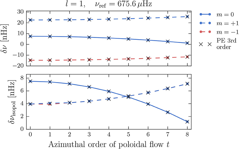
Figure 6. Frequency shifts in the co-rotating frame for the almost pure p-type l = 1 multiplet at 675.6 μHz. (Upper) Shifts resulting from rotation combined with a poloidal flow of s = 8 and different values of t. (Lower) Isolated frequency shifts due to the poloidal flow.

5.1.4. Modes of Degree l = 2

For modes of harmonic degree l = 2 distinguishing between p-type and g-type modes becomes necessary, since the results differ substantially.

Figure 7 displays the frequency shifts in the co-rotating frame for an l = 2 multiplet of g-type with an original frequency of 659.3 μHz for different poloidal flow configurations. From the upper panel, showing the shifts due to the combined effect of rotation and the poloidal flow, it is evident that the multiplet is strongly affected by the fast rotating core, leading to a clearly antisymmetric splitting of the modes of different azimuthal order m. Even in the frame of reference that is co-rotating with the envelope angular velocity, the splitting of the multiplet is very strong, amounting up to several hundred nHz. This causes the contribution of the poloidal flow to be not discernible at all in the upper panel, which is evident from the fact that the shifts do not seem to change for different cell configurations t. In the lower panel of Figure 7, where the effect of rotation is subtracted (cf. Equation 44), the t-dependence of the shifts becomes visible. The remaining frequency shifts, which are only of the order of a few nHz, show a notable asymmetry in ±m that persists for all configurations t. This asymmetry is well-reproduced by the results obtained with the PE method and originates from a strong third order contribution.

FIGURE 7

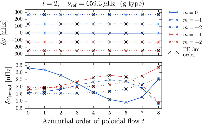
Figure 7. Frequency shifts for the g-type l = 2 multiplet at 659.3 μHz in the co-rotating frame. (Upper) Shifts resulting from rotation combined with a poloidal flow of s = 8 and different values of t. (Lower) Isolated frequency shifts of the poloidal flow.

In Figure 8, frequency shifts in the co-rotating frame for a p-type l = 2 multiplet with an original frequency of 701.3 μHz are displayed. In contrast to the g-type multiplet, the combined splitting of rotation and poloidal flow is much weaker (upper panel) and the different azimuthal order components are not clearly separated for every t. This is due to the fact, that for the p-type multiplet, the effect of rotation does not outperform the effect of the poloidal flow, but instead they are of similar magnitude, since the p-type multiplet has only a low sensitivity to the fast rotating core. The weak rotational influence leads to asymmetries in the frequency shifts caused by degenerate coupling, which are best visible in the lower panel of Figure 7, where the isolated frequency shifts due to the poloidal flow are displayed. For most of the flow configurations t, the shifts are symmetric in ±m, but for t = 1 and t = 2 there are asymmetries in the shifts for modes with m = ±1 and m = ±2, respectively, which are not reproduced by the PE method. From the lower panel it is also evident that, compared to the g-type multiplet, the third order contribution for the p-type multiplet is small enough to not cause any notable asymmetry.

FIGURE 8

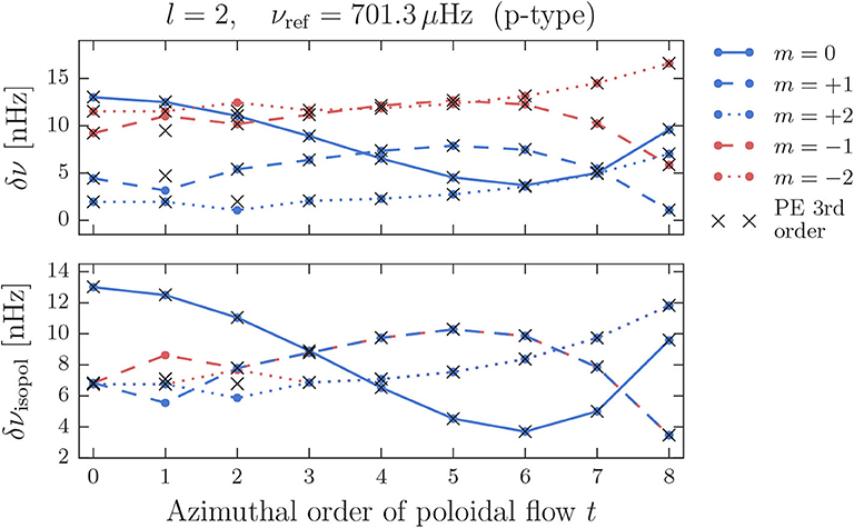
Figure 8. Frequency shifts for the p-type l = 2 multiplet at 701.3 μHz in the co-rotating frame. (Upper) Shifts resulting from rotation combined with a poloidal flow of s = 8 and different values of t. (Lower) Isolated frequency shifts of the poloidal flow.

5.1.5. Summary of the Results on Frequency Shifts

Subgiant stars harbor mixed modes that can be of p- or of g-type. Modes with l = 0 are pure p modes, and in the subgiant model selected here, modes with l = 1 have sensitivity in the convection zone. The first pronounced g-type modes start to appear at l = 2 (cf. Figure 1). From an observational point of view, however, they might have low amplitudes. Different mode types are prone to different causes of asymmetry in the frequency shifts for modes of opposite azimuthal order ±m. Modes of g-type have a high sensitivity to the conditions in the core region. For models with a fast rotating core and a poloidal flow in the convection zone, this leads to a significant third order eigenvalue correction, causing an asymmetry in the shifts.

Modes of p-type are less sensitive to the core region, leading to a smaller effect of rotation for models where merely a fast rotating core is prescribed. A small rotational effect yields an insufficient lifting of the degeneracy in first order, so that the degenerate coupling occurring in second order (due to the poloidal flow) retains a notable influence and causes an asymmetry in the frequency shifts. This effect can only occur for modes that are part of degenerate coupling sets.

From the examples shown in the preceding sections it is evident that both discussed types of asymmetries are significantly smaller than the actual frequency shifts induced by the poloidal flow.

In general we note, that the frequency shifts calculated for the models above are small and difficult to detect. Therefore, in addition to the frequency shift, we take the perturbation of the eigenfunctions in the following sections into account.

5.2. The Multiperiodic Signal in an Inertial Frame

Since observations are typically carried out from a stationary observer's frame of reference, the results obtained in the co-rotating frame have to be transformed into an inertial reference frame. This transformation and its effect on the eigenfunctions is discussed in section 5.2.1. The transformation of coordinate systems will result in a multiperiodic observational signal for each perturbed mode in the inertial frame, which is derived in section 5.2.2. In section 5.2.3 exemplary results for this signal are presented.

For the calculation of multiperiodic signals the amplified flow velocity profile is adopted that was also used for the calculation of frequency shifts (cf. section 5.1). For the cell configuration of the poloidal flow we adopt a configuration with s = 8 and different values of t, including meridional (t = 0) and sectoral (t = s) cells.

5.2.1. Transformation From a Co-rotating to an Inertial Frame

We employ a transformation from a co-rotating reference frame to an inertial frame as discussed in Lavely and Ritzwoller (1992). Given a star rotating with uniform angular velocity Ω, we define two sets of spherical polar coordinates, coordinates (r_R, θ_R, ϕ_R) in the frame co-rotating with the star and coordinates (r_I, θ_I, ϕ_I) in an inertial frame. The two sets of coordinates are related by

$\begin{array}{ll}(r_R,{\theta }_R,{\varphi }_R)=(r_I,{\theta }_I,{\varphi }_I-\Omega t).& (45)\end{array}$

We now wish to transform a perturbed mode of oscillation ${\tilde{\xi }}_k^R$ from the co-rotating frame to the inertial frame

$\begin{array}{ll}{\tilde{\xi }}_k^R(r_R,{\theta }_R,{\varphi }_R,t)={\tilde{\xi }}_k^R(r_I,{\theta }_I,{\varphi }_I-\Omega t,t)={\tilde{\xi }}_k^I(r_I,{\theta }_I,{\varphi }_I,t).& (46)\end{array}$

Perturbation theory yields perturbed modes that can be expressed as linear combinations of the unperturbed modes (cf. Equation 24)

$\begin{array}{ll}{\tilde{\xi }}_k^R(r_R,{\theta }_R,{\varphi }_R,t)=\left[{\displaystyle \sum _{j\in K}}{a}_j^k{\xi }_j^R(r_R,{\theta }_R,{\varphi }_R)\right]{\text{e}}^{-i{\tilde{\omega }}_{k}t},& (47)\end{array}$

where we have assumed the simple time dependence of a harmonic oscillation. The quantity in square brackets, which represents the eigenfunction of the perturbed mode k, is time-independent in the co-rotating frame, meaning the spatial pattern oscillating with perturbed frequency ${\tilde{\omega }}_k$ remains the same for all time, when observed while co-rotating with the star. Inserting Equation (46) into Equation (47) yields the expression for the mode in the inertial frame

$\begin{array}{ll}{\tilde{\xi }}_k^R(r_I,{\theta }_I,{\varphi }_I-\Omega t,t)=\left[{\displaystyle \sum _{j\in K}}{a}_j^k{\xi }_j^R(r_I,{\theta }_I,{\varphi }_I-\Omega t)\right]{\text{e}}^{-i{\tilde{\omega }}_{k}t}& (48)\\ =\left[{\displaystyle \sum _{j\in K}}{a}_j^k{\xi }_j^R(r_I,{\theta }_I,{\varphi }_I){\text{e}}^{-i{m}_j\Omega t}\right]{\text{e}}^{-i{\tilde{\omega }}_{k}t}& (49)\\ ={\displaystyle \sum _{j\in K}}{a}_j^k{\xi }_j^R(r_I,{\theta }_I,{\varphi }_I){\text{e}}^{-i({\tilde{\omega }}_k+m_j\Omega )t},& (50)\end{array}$

where we have used the fact that the azimuthal dependence of the eigenfunctions is given by e^imϕ, stemming from spherical harmonics (cf. Equation 3). We added the subscript j at the azimuthal order to indicate the corresponding multiplet. The expressions above show that, in the inertial frame, the spatial pattern that oscillates with frequency ${\tilde{\omega }}_k$ actually changes with time, since the eigenfunctions have acquired a time dependence (Equation 49). In other words, the oscillation originating from one perturbed mode in the co-rotating frame, is multiply periodic in the inertial frame (Equation 50), whereby the number of different frequencies depends on the number of different azimuthal orders m contributing to the coupling of the perturbed mode.

5.2.2. The Signal to Be Observed in an Inertial Frame

In the co-rotating frame, the velocity field generated by a perturbed mode k, with eigenfunction ${\tilde{\xi }}_k(r,\theta ,\varphi )$ and eigenfrequency ${\tilde{\omega }}_k$, can be written as

$\begin{array}{ll}{v}_k(r,\theta ,\varphi ,t)={\alpha }_k(t){\text{e}}^{-i{\tilde{\omega }}_{k}t}{\tilde{\xi }}_k={\alpha }_k(t){\text{e}}^{-i{\tilde{\omega }}_{k}t}{\displaystyle \sum _{j\in K}}{a}_j^k{\xi }_j,& (51)\end{array}$

where α_k(t) is a time dependent amplitude of the oscillatory velocity field, incorporating excitation and damping effects, and the ξ_j denote the unperturbed eigenfunctions (cf. Equation 3) of the oscillation modes in set K. For low to intermediate harmonic degrees l, the horizontal component of the vector field (3) at the surface is much smaller than the radial component, ξ^h(R) ≪ ξ^r(R) (e.g., for the solar 5-min oscillations ξ^h(R)/ξ^r(R) ~ 0.001, Aerts et al., 2010), so the motion is predominantly vertical. Therefore, the velocity field at the surface is approximately given by

$\begin{array}{ll}{v}_k(R,\theta ,\varphi ,t)={\alpha }_k(t){\text{e}}^{-i{\tilde{\omega }}_{k}t}{\displaystyle \sum _{j\in K}}{a}_j^k{\xi }_j^r(R)Y_l^m(\theta ,\varphi )e_r.& (52)\end{array}$

This is valid in the co-rotating frame, where the poloidal flow cells are stationary. To calculate the signal of the velocity field observed in a stationary reference frame, we need to employ the transformation (Equation 46); thereby the velocity field in the inertial frame becomes

$\begin{array}{ll}{v}_k^I(R_I,{\theta }_I,{\varphi }_I,t)=v_k(R_I,{\theta }_I,{\varphi }_I-\Omega t,t)& (53)\\ ={\alpha }_k(t){\text{e}}^{-i{\tilde{\omega }}_{k}t}{\displaystyle \sum _{j\in K}}{a}_j^k{\xi }_j^r(R)Y_l^m({\theta }_I,{\varphi }_I-\Omega t)e_r& (54)\\ ={\alpha }_k(t){\text{e}}^{-i{\tilde{\omega }}_{k}t}{\displaystyle \sum _{j\in K}}{a}_j^k{\xi }_j^r(R)Y_l^m({\theta }_I,{\varphi }_I){\text{e}}^{-im\Omega t}{e}_r.& (55)\end{array}$

We now discard the unit vector e_r and further examine merely the scalar value of the velocity field, which is tantamount to ideal observation conditions, where the full stellar surface would be observed. For realistic observation conditions, further projection effects and consideration of mode visibilities have to be taken into account (cf. Dziembowski, 1977; Schad, 2011). Additionally, we merge the exponential time dependences. This yields

$\begin{array}{ll}{v}_k^I(R_I,{\theta }_I,{\varphi }_I,t)={\alpha }_k(t){\displaystyle \sum _{j\in K}}{a}_j^k{\xi }_j^r(R)Y_l^m({\theta }_I,{\varphi }_I){\text{e}}^{-i({\tilde{\omega }}_k+m\Omega )t}.& (56)\end{array}$

Projecting the velocity field $v_k^I(R_I,{\theta }_I,{\varphi }_I,t)$ onto the different occurring $Y_l^m$, by multiplying Equation (56) with the corresponding complex conjugate spherical harmonic ${(Y_l^m)}^{*}$ and integrating over the full solid angle, we obtain the signal component of each spherical harmonic comprising the surface velocity signal in the observer's frame

$\begin{array}{ll}{y}_{lm}^k(t)={\alpha }_k(t){\displaystyle \sum _{j\in K_{lm}}}{a}_j^k{\xi }_j^r(R){\text{e}}^{-i({\tilde{\omega }}_k+m\Omega )t}.& (57)\end{array}$

Here, the set K_lm ⊂ K now consists only of modes that have the same harmonic degree l and azimuthal order m, but different radial orders n. Each spherical harmonic component of the velocity signal, as given by Equation (57), essentially consists of an amplitude and frequency. Since the time dependent amplitude α_k(t) in general might not be known, it is more convenient to work with relative, instead of absolute amplitudes for the different components. Therefore, we define a new quantity ${\psi }_{lm}^k(t)$ that is obtained by dividing Equation (57) by the amplitude ${\alpha }_k(t)a_k^k{\xi }_k^r(R)$ of the reference mode component of the signal, yielding

$\begin{array}{ll}{\psi }_{lm}^k(t)={\displaystyle \sum _{j\in K_{lm}}}{A}_{kj}\frac{{\xi }_j^r(R)}{{\xi }_k^r(R)}{\text{e}}^{-i({\tilde{\omega }}_k+m\Omega )t},& (58)\end{array}$

where the A_kj are so-called coupling ratios as introduced by Schad (2011), which are defined as

$\begin{array}{ll}{A}_{kj}=\frac{a_j^k}{a_k^k}.& (59)\end{array}$

Applying a Fourier transform to Equation (58), we obtain explicit frequency positions and corresponding relative amplitudes of the different signal components:

$\begin{array}{ll}{\widehat{\psi }}_{lm}^k(\omega )={\displaystyle \sum _{j\in K_{lm}}}{A}_{kj}\frac{{\xi }_j^r(R)}{{\xi }_k^r(R)}\delta (\omega -({\tilde{\omega }}_k+m\Omega )).& (60)\end{array}$

Here, δ(ω) denotes the Dirac delta function, which is non-zero only at ω = 0. We will use the quantities in the equation above, to showcase the effect of the flow which is to be observed in an inertial frame. Specifically, we will display the absolute value of the complex relative amplitude

$\begin{array}{ll}{\eta }_{lm}^k:=\left|{\displaystyle \sum _{j\in K_{lm}}}{A}_{kj}\frac{{\xi }_j^r(R)}{{\xi }_k^r(R)}\right|& (61)\end{array}$

for the different spherical harmonics and frequencies that compose the multiperiodic signal in the observer's frame.

5.2.3. Multiperiodic Signal of an l = 1 Multiplet

The multiperiodic signal, or more specifically the frequencies and relative amplitudes ${\eta }_{lm}^k$ of the different spherical harmonic components of the multiperiodic signal, which are generated by a perturbed multiplet of harmonic degree l = 1 in a stationary observer's frame, are shown in Figure 9. Each panel shows the result for a different flow cell configuration t, including also a meridional flow (t = 0, top panel) and sectoral cells (t = s = 8, bottom panel). The signal components (dots) are separated by harmonic degree l, which is given on the ordinate, and by frequency given on the abscissa. The dot size (area) expresses the modulus of the complex amplitude ${\eta }_{lm}^k$ (cf. Equation 61) of the different signal components relative to the reference modes. The three largest dots represent the reference mode components of the signal with l = 1 and m = −1, 0, +1, plus three further coupling modes of the same l and m but different radial order n that are part of the coupling set. The azimuthal order m, which causes the multiperiodicity of the signal, is indicated by the dot color. The frequency of the unperturbed multiplet is marked by a vertical dotted line.

FIGURE 9

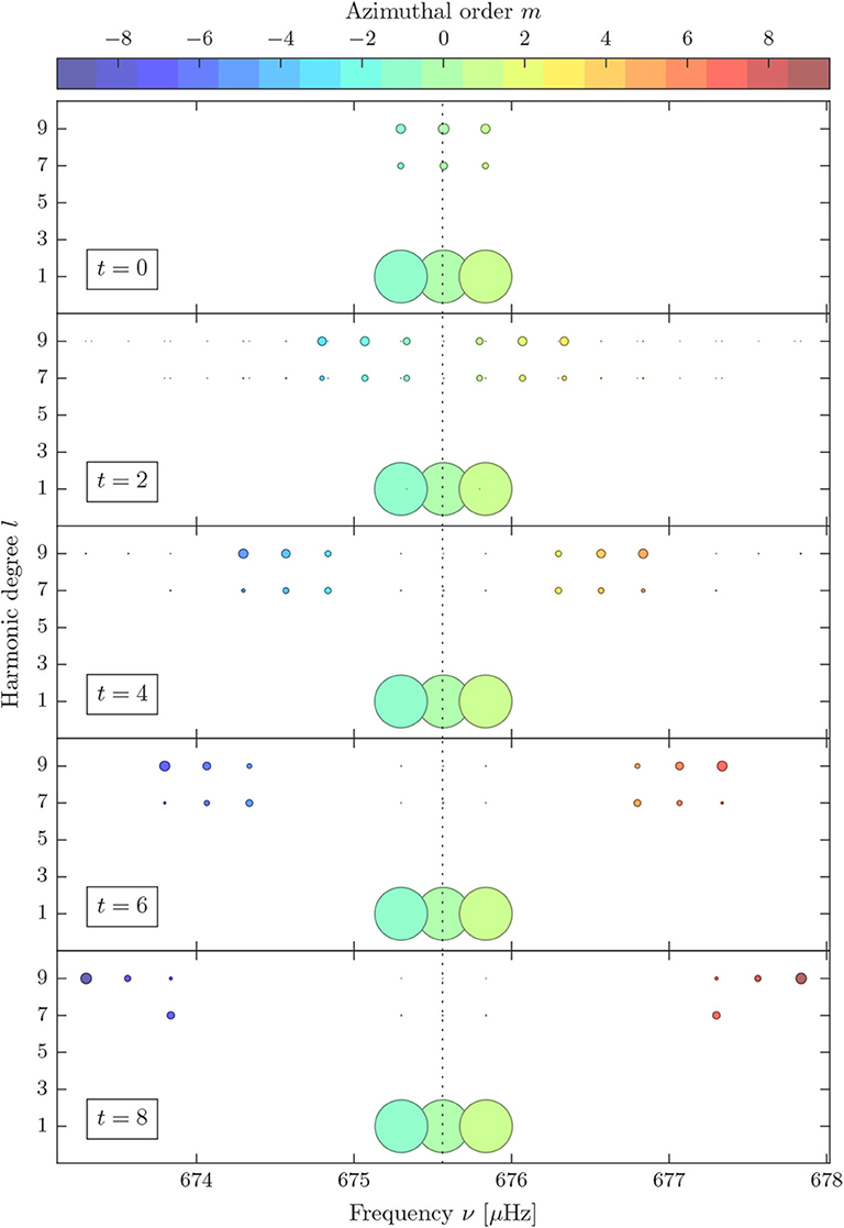
Figure 9. Frequencies and relative amplitudes ${\eta }_{lm}^k$ (dot size) of the multiperiodic signal for the perturbed l = 1 multiplet in a stationary observer's frame for a poloidal flow with s = 8, t = 0, 2, 4, 6, 8 and an amplified flow profile. Dot colors indicate different values of m. The dotted line marks the unperturbed multiplet frequency ν_ref = 675.6 μHz.

For an axisymmetric (meridional) flow, given in the top panel of Figure 9, we see that the originally degenerate multiplet is split into its three azimuthal order components m = −1, m = 0, and m = +1 in frequency. Note, that this frequency splitting is not equal to the splitting shown for t = 0 in the upper panel of Figure 6, but is much stronger, since the transformation into the observer's frame adds an additional mΩ_sys to the frequency shift of each mode. The asymmetry induced by the poloidal flow, which is visible in the co-rotating frame (cf. Figure 6, upper panel), is almost undetectable in the observer's frame. There, the frequency shifts are dominated by the contribution to the shift arising from the switch of reference frames, which is antisymmetric in ±m.

As s = 8 and because of Equation (21), apart from the dominant reference mode component, the signal in the observer's frame of each of the three perturbed modes contains additional components with harmonic degree l = 7 and l = 9, which are of lower amplitude. For t = 0, these components oscillate with the same frequency as their respective reference mode component (cf. Figure 9, top panel). This is due to the fact that axisymmetric flows couple only modes of the same azimuthal order m, and m determines the frequencies observed in the stationary observer's frame (cf. Equation 60). So, even though the multiplet splits into three modes of different azimuthal order due to the perturbation and the frame switch, each of these three individual perturbed modes remains monoperiodic in the observer's frame for t = 0.

For non-axisymmetric flows (t ≠ 0), shown in the remaining panels of Figure 9, the additional l = 7 and l = 9 components acquire frequencies different from the reference mode components, so the signal of each reference mode becomes multiperiodic. For each reference mode, there are two dominant ancillary signal components per harmonic degree l, and several minuscule components. The two dominant components, one of which has a higher frequency than the reference mode component and one has a lower frequency, correspond to modes of azimuthal order m = m_ref ± t, which couple directly to the reference mode. The minuscule components result from secondary and higher order couplings. With increasing t, the dominant ancillary components migrate away from the reference mode components, to higher and lower frequencies, respectively. This migration is due to the fact that, with increasing t, the poloidal flow couples the reference mode to modes whose azimuthal order m differs more strongly from the azimuthal order of the reference mode [cf. selection rule (22)].

Overall we find, that due to mode coupling the individual perturbed modes have frequency contributions from all modes in the coupling set. Hence, high-degree modes add frequency contributions to the signal of low degree modes and vice versa in the presence of a suitable velocity field. As a result, the perturbed oscillation will be a beating. This leads to sidelobes in the respective power spectrum. Those sidelobes, which are then appearing due to mode coupling to high-degree modes are potentially measurable signatures in the power spectra obtained from asteroseismic time series. These sidelobes carry characteristic information about the large-scale flow components present inside a star.

6. Summary and Discussion

By means of forward calculations we investigated the effects of large-scale poloidal flows on the frequencies and eigenfunctions of stellar oscillation modes for a subgiant star, in the non-rotating and the rotating case. The work focused in particular on axisymmetric (t = 0) and non-axisymmetric (t ≠ 0) flow configurations, associated with meridional flows and giant cells, respectively. The results were obtained by applying perturbation theory based on Lavely and Ritzwoller (1992), where the flow is treated as a perturbation of an equilibrium stellar model, which leads to a coupling of the oscillation modes, which in turn results in frequency shifts and a mixing of the mode eigenfunctions.

6.1. Non-rotating Case

For the non-rotating case, we find that the frequency shifts caused by any poloidal flow (axi- and non-axisymmetric) are symmetric for modes of opposite azimuthal order ±m, provided no degeneracy occurs, i.e., the modes in the reference multiplet form non-degenerate coupling sets. If the reference modes form degenerate coupling sets, a circumstance which can only arise for non-axisymmetric flow configurations, the frequency shifts of modes of opposite azimuthal order ±m are asymmetric, and the modes that experience the shifts are mixtures of oscillation states that do not possess a well-defined azimuthal order.

We investigated the behavior of the frequency shift depending on the flow's azimuthal order t and harmonic degree s. The parameter t changes the position of the shifted modes within the multiplet relative to each other, a behavior which is governed by the Wigner-3j symbols. The parameter s causes an overall change in the frequency shift for the entire multiplet, but there is no distinct trend of the shift with s visible.

For the low degree modes considered here, the frequency shifts caused by the flows are predominantly positive. The magnitude of the shifts is of the order of 10⁻¹ nHz to 1 nHz, varying for different frequencies. Unfortunately, this magnitude is one to two orders of magnitude lower than typical errors on measured oscillation frequencies. For example, the frequency errors obtained from Kepler data for several subgiant and young red giant stars (Deheuvels et al., 2014) are of the order of 10⁻² μHz. We therefore could conclude that the small shifts induced by purely poloidal flows will not be detectable in subgiant stars, considering current analysis methods and assuming flow velocities comparable to the ones prescribed in this work. Nevertheless, considering modes in subgiants with partial g-mode behavior, that therefore have a narrower peak in the power spectrum and smaller errors of frequencies might be close to the detection of the frequency shifts.

6.2. Rotating Case

In the rotating case, it is possible for the frequency shifts of modes of opposite azimuthal order ±m to show two different types of asymmetries of different origin. If the star possesses a fast rotating core, the frequency shift of g-type modes acquires a significant third order contribution, causing an asymmetry. For p-type modes, on the other hand, substantial residual degenerate coupling can lead to an asymmetry, which occurs when rotation is not able to lift an existing degeneracy sufficiently. The frequency shifts remain of the same order of magnitude as in the non-rotating case and are therefore not a suitable measure to detect large-scale flows.

However, in a stationary observer's frame, the mode mixing induced specifically by non-axisymmetric poloidal flows causes each perturbed mode to appear as a multiperiodic observational signal. We derived an expression for the amplitudes of the different signal components and presented the pattern of the signal as a function of frequency and harmonic degree. Apart from the reference mode component of the signal, which possesses the highest amplitudes, several low-amplitude ancillary signal components with different frequencies appear (two dominant ancillary components per reference mode and coupling harmonic degree). The amplitudes of these ancillary components are sensitive to the flow. For distant stars, only low-degree modes (l ≤ 3) can be observed in oscillation spectra. The ancillary components of low-degree modes are, for most flow configurations, of harmonic degree l′ > 3 [cf. selection rule (21)] and are therefore, due to unresolved stellar surfaces, most likely undetectable in current stellar data. However, the problem can be considered the other way around: Due to mode coupling the higher degree modes leave their imprint in the lowest degree modes, too. The degrees best visible in stellar data are l = 0 and l = 1. For a poloidal flow of given degree s, the triangle inequality (Equation 21) yields that the perturbed multiplets of degrees l′ = s, l′ = s − 1, and l′ = s + 1 will create ancillary signal components in the time series of the modes with degrees l = 0 or l = 1. Therefore, the most promising procedure to detect signatures of a specific poloidal flow field in stellar oscillation spectra would be to search for unidentified peaks (ancillary signal components) at frequencies belonging to the aforementioned modes of degrees l′ = s, s − 1, s + 1.

Generally, this study could be expanded to other stars of different masses and evolutionary stages. Obviously, real large-scale stellar velocity fields are a superposition of several flow components, which therefore all of them would lead to side lobes in the power spectrum of low-degree modes. Supported by more realistic models of stellar convection, actual potential detection limits of large-scale flows in stars by asteroseismology could be derived. We defer such studies to later investigations.

We would also like to note that in turn, if such side lobes in the power spectrum could be detected, they would provide hints on the frequencies of the high-degree modes, too. This would therefore support the modeling of the respective star.

Data Availability Statement

The datasets generated for this study are available on request to the corresponding author.

Author Contributions

WH carried out the calculations, prepared the plots, and contributed to drafting the manuscript. MR initiated the study, supervised WH, contributed to the drafting of the text, and completed the manuscript.

Funding

The research leading to this result has received funding from the European Research Council under the European Union's Seventh Framework Program (FP/2007-2013)/ERC Grant Agreement No. 307117.

Conflict of Interest

The authors declare that the research was conducted in the absence of any commercial or financial relationships that could be construed as a potential conflict of interest.

Acknowledgments

Parts of the work presented here appeared in WH's thesis (Herzberg, 2016) to obtain a doctoral degree at the Albert-Ludwigs-Unviversität Freiburg.

References

Aerts, C., Christensen-Dalsgaard, J., and Kurtz, D. W. (2010), “Asteroseismology,” in Asteroseismology, Astronomy Astrophysics Library (Springer Science+Business Media B.V.). Available online at: https://ui.adsabs.harvard.edu/#abs/2010aste.book.A/abstract

Google Scholar

Böhm-Vitense, E. (1958). Über die Wasserstoffkonvektionszone in Sternen verschiedener Effektivtemperaturen und Leuchtkräfte. Z. Astrophys. 46:108.

Google Scholar

Chatterjee, P., and Antia, H. M. (2009). Solar flows and their effect on frequencies of acoustic modes. Astrophys. J. 707, 208–217. doi: 10.1088/0004-637x/707/1/208

CrossRef Full Text | Google Scholar

Christensen-Dalsgaard, J. (2008). ADIPLS–the Aarhus adiabatic oscillation package. Astrophys. Space Sci. 316, 113–120. doi: 10.1007/s10509-007-9689-z

CrossRef Full Text | Google Scholar

Dahlen, F. A., and Tromp, J. (1998). Theoretical Global Seismology. Princenton, NJ: Princeton University Press.

Google Scholar

Deheuvels, S., Dogan, G., Goupil, M. J., Appourchaux, T., Benomar, O., Bruntt, H., et al. (2014). Seismic constraints on the radial dependence of the internal rotation profiles of six Kepler subgiants and young red giants. Astron. Astrophys. 564:A27. doi: 10.1051/0004-6361/201322779

CrossRef Full Text | Google Scholar

Dupret, M. -A., Belkacem, K., Samadi, R., Montalban, J., Moreira, O., Miglio, A., et al. (2009). Theoretical amplitudes and lifetimes of non-radial solar-like oscillations in red giants. Astron. Astrophys. 506, 57–67. doi: 10.1051/0004-6361/200911713

CrossRef Full Text | Google Scholar

Dziembowski, W. (1977). Oscillations of giants and supergiants. Acta Astron. 27, 95–126.

Google Scholar

Edmonds, A. (1960). Angular Momentum in Quantum Mechanics. Investigations in Physics. Princeton, NJ: Princeton University Press.

Google Scholar

Greer, B. J., Hindman, B. W., Featherstone, N. A., and Toomre, J. (2015). Helioseismic imaging of fast convective flows throughout the near-surface shear layer. Astrophys. J. Lett. 803:L17. doi: 10.1088/2041-8205/803/2/l17

CrossRef Full Text | Google Scholar

Hanasoge, S. M., Duvall, T. L., and Sreenivasan, K. R. (2012). Anomalously weak solar convection. Proc. Natl. Acad. Sci. U.S.A. 109, 11928–11932. doi: 10.1073/pnas.1206570109

PubMed Abstract | CrossRef Full Text | Google Scholar

Hanasoge, S. M., and Sreenivasan, K. R. (2014). The quest to understand supergranulation and large-scale convection in the sun. Solar Phys. 289, 3403–3419. doi: 10.1007/s11207-014-0471-4

CrossRef Full Text | Google Scholar

Hathaway, D. H., Upton, L., and Colegrove, O. (2013). Giant convection cells found on the sun. Science 342, 1217–1219. doi: 10.1126/science.1244682

PubMed Abstract | CrossRef Full Text | Google Scholar

Herzberg, W. (2016). Effects of large-scale poloidal flows on oscillation modes of subgiant stars and the sun (Ph.D. thesis), Albert-Ludwigs-Universität Freiburg, Freiburg, Germany.

Google Scholar

Lavely, E. M., and Ritzwoller, M. H. (1992). The effect of global-scale, steady-state convection and elastic-gravitational asphericities on helioseismic oscillations. Philos. Trans. R. Soc. 339:1655.

Google Scholar

López Ariste, A., Mathias, P., Tessore, B., Lèbre, A., Aurière, M., Petit, P., et al. (2018). Convective cells in Betelgeuse: imaging through spectropolarimetry. Astron. Astrophys. 620:A199. doi: 10.1051/0004-6361/201834178

CrossRef Full Text | Google Scholar

Miesch, M. S. (2005). Large-scale dynamics of the convection zone and tachocline. Living Rev. Sol. Phys. 2:1. doi: 10.12942/lrsp-2005-1

CrossRef Full Text | Google Scholar

Montargès, M., Norris, R., Chiavassa, A., Tessore, B., Lèbre, A., et al. (2018). The convective photosphere of the red supergiant CE Tauri. I. VLTI/PIONIER H-band interferometric imaging. Astron. Astrophys. 614:12. doi: 10.1051/0004-6361/201731471

CrossRef Full Text | Google Scholar

Paxton, B. (2011). Modules for experiments in stellar astrophysics (MESA). Astrophys. J. Suppl. 192:3. doi: 10.1088/0067-0049/192/1/3

PubMed Abstract | CrossRef Full Text | Google Scholar

Ritzwoller, M. H., and Lavely, E. M. (1991). A unified approach to the helioseismic forward and inverse problems of differential rotation. Astrophys. J. 369, 557–566.

Google Scholar

Roth, M., Howe, R., and Komm, R. (2002). Detectability of large-scale flows in global helioseismic data - A numerical experiment. Astron. Astrophys. 396, 243–253. doi: 10.1051/0004-6361:20021358

CrossRef Full Text | Google Scholar

Roth, M., and Stix, M. (1999). Coupling of solar p modes: quasi-degenerate perturbation theory. Astron. Astrophys. 351, 1133–1138.

Google Scholar

Roth, M., and Stix, M. (2008). Meridional circulation and global solar oscillations. Solar Phys. 251, 77–89. doi: 10.1007/s11207-008-9232-6

CrossRef Full Text | Google Scholar

Ruediger, G. (1989). Differential Rotation and Stellar Convection. Sun and the Solar Stars. Berlin: Akademie Verlag.

Google Scholar

Sakurai, J. J., and Napolitano, J. (2011). Modern Quantum Mechanics, 2nd Edn. London: Addison Wesley.

Google Scholar

Schad, A. (2013). A new approach for the global helioseismic investigation of the solar meridional flow (Ph.D. thesis), Albert-Ludwigs-Universitaet Freiburg im Breisgau, Freiburg, Germany.

Schad, A., Timmer, J., and Roth, M. (2011). A unified approach to the helioseismic inversion problem of the solar meridional flow from global oscillations. Astrophys. J. 734:97. doi: 10.1088/0004-637X/734/2/97

CrossRef Full Text | Google Scholar

Schiff, L. (1968). Quantum Mechanics. New York, NY: McGraw-Hill.

Trampedach, R., Asplund, M., Collet, R., Nordlund, A., and Stein, R. F. (2013). A grid of three-dimensional stellar atmosphere models of solar metallicity. I. General properties, granulation, and atmospheric expansion. Astrophys. J. 769:18.

Google Scholar

Tremblay, P.-E., Ludwig, H.-G., Freytag, B., Steffen, M., and Caffau, E. (2013). Granulation properties of giants, dwarfs, and white dwarfs from the CIFIST 3D model atmosphere grid. Astron. Astrophys. 557:A7. doi: 10.1088/0004-637x/769/1/18

CrossRef Full Text | Google Scholar

Woodhouse, J. H. (1980). The coupling and attenuation of nearly resonant multiplets in the Earth's free oscillation spectrum. Geophys. J. 61, 261–283.

Google Scholar

7. Appendix

7.1. Flow Kernels

Expressions for the flow kernels as given by Lavely and Ritzwoller (1992):

$\begin{array}{l}{R}_s(r)=\frac{1}{2}\left({{\xi }^r}^{\prime }\frac{\text{d}{\xi }^r}{\text{d}r}-\frac{\text{d}{{\xi }^r}^{\prime }}{\text{d}r}{\xi }^r\right)B_{l^{\prime }sl}^{(0)+}\\ \begin{array}{l}+\frac{1}{2}\left({{\xi }^h}^{\prime }\frac{\text{d}{\xi }^h}{\text{d}r}-\frac{\text{d}{{\xi }^h}^{\prime }}{\text{d}r}{\xi }^h\right)B_{l^{\prime }sl}^{(1)+},\end{array}& (\mathrm{A1})\end{array}$

$\begin{array}{l}{H}_s(r)=\frac{1}{2r}\left[l(l+1)-l^{\prime }(l^{\prime }+1)\right]·\left[{{\xi }^r}^{\prime }{\xi }^r{B}_{l^{\prime }sl}^{(0)+}+{{\xi }^h}^{\prime }{\xi }^h{B}_{l^{\prime }sl}^{(1)+}\right]\\ \begin{array}{l}+\frac{1}{r}{{\xi }^h}^{\prime }{\xi }^r{B}_{l^{\prime }ls}^{(1)+}-\frac{1}{r}{{\xi }^r}^{\prime }{\xi }^h{B}_{l{l}^{\prime }s}^{(1)+},\end{array}& (\mathrm{A2})\end{array}$

$\begin{array}{l}{T}_s(r)=\frac{1}{r}\{{{\xi }^r}^{\prime }{\xi }^h+{{\xi }^h}^{\prime }{\xi }^r-{{\xi }^r}^{\prime }{\xi }^r\\ -\frac{1}{2}{{\xi }^h}^{\prime }{\xi }^h\left[l(l+1)+l^{\prime }(l^{\prime }+1)-s(s+1)\right]\}{B}_{l^{\prime }sl}^{(1)-},& (\mathrm{A3})\end{array}$

where the coefficients $B_{ijk}^{(N)\pm }$ are defined by Woodhouse (1980):

$\begin{array}{l}{B}_{ijk}^{(N)\pm }=\frac{1}{2}\left[1\pm {(-1)}^{(i+j+k)}\right]·{\left[\frac{(i+N)!(k+N)!}{(i-N)!(k-N)!}\right]}^{\frac{1}{2}}{(-1)}^N\\ \begin{array}{l}·\left(\begin{array}{ccc}i& j& k\\ -N& 0& N^{\prime }\end{array}\right).\end{array}& (\mathrm{A4})\end{array}$

The coefficients $B_{ijk}^{(N)\pm }$ satisfy several useful identities, in particular we employed

$\begin{array}{ll}{B}_{ijk}^{(1)+}=\frac{1}{2}\left[i(i+1)+k(k+1)-j(j+1)\right]B_{ijk}^{(0)+}& (\mathrm{A5})\end{array}$

and

$\begin{array}{l}{B}_{ijk}^{(1)-}=\frac{1}{2}[\frac{(\Sigma +2)(\Sigma +4)}{\Sigma +3}\\ {(\Sigma +1-2k)(\Sigma +1-2i)(\Sigma +1-2j)]}^{\frac{1}{2}}\\ ·B_{i+1,j+1,k+1}^{(0)+},& (\mathrm{A6})\end{array}$

with Σ = i + j + k.