Testing and Validating Two Morphological Flare Predictors by Logistic Regression Machine Learning

1 Introduction

A solar flare is a sudden flash observed in the solar atmosphere which is able to rapidly heat the plasma to megakelvin temperatures, while the electrons, protons and other heavier ions are accelerated to very large speeds (Benz, 2008). The associated accelerated particle clouds may reach the Earth, typically within a few hours or a day following a solar flare eruption. The flares produce radiation across the electromagnetic spectrum at all wavelengths. Most of the released energy is spread over frequencies outside the visible range. For this reason, the majority of flares must be observed with instruments which measurements in these wavelength ranges, as e.g., the Geostationary Operational Environmental Satellite (GOES). Therefore, the most generally known flare classification scheme is GOES flare-class. Measurements of the maximum x-ray flux at wavelengths from 0.1 to 0.8 nm near Earth are classed as A, B, C, M, or X type flares back from 1975¹. These five GOES flare intensity categories are further divided into a logarithmic scale labeled from 1 to 9. The A-, B- and C-classes are the lowest energy release classes of solar flares and they also occur frequently in the solar atmosphere. The A to C-class range has no or hardly any detectable effect on Earth based on current instrumentations and understanding. The M-class medium flare category may cause smaller or occasionally more serious disruptions, e.g., radio blackouts. However, the X-intensity flares may cause strong to extreme hazardous events, facility break-downs (e.g., radio blackouts, etc.) on the daylight side of the Earth (Hayes et al., 2017). The major solar flares (M- and X-class) are often accompany with accelerated solar energetic particles and coronal mass ejections (CMEs) (see, e.g.,, Tziotziou et al., 2010).

For solar activity modeling, a key ingredient is to determine the role of the associated observable magnetic field. Waldmeier (1938) proposed the first classification scheme to examine the connection between the size and morphology of active regions (ARs) and the capacity of their flare-productivity. This classification scheme is known today as the Zürich classification (see also Kiepenheuer, 1953). This scheme contains eight types thought to be representative of consecutive states in the evolution of a sunspot group. The classification system was further developed by McIntosh (1990). McIntosh introduced three more components based on characteristics including the Zürich class, the largest sunspot, and the sunspot distribution in an AR. Although the classification uses white-light observations only, it is still widely used.

The first magnetic classification scheme, known as the Mount Wilson classification, was introduced by Hale et al. (1919). It is simpler than the Zürich-McIntosh system, as it only distinguishes unipolar, bipolar, mixed configurations and very close and mixed configurations within a common penumbral feature, denoted by the letters α, β, γ and δ-class, respectively. Künzel (1960) added the δ-class configurations for the McIntosh system which refer to the most productive sources of energetic flares (see, e.g.,, Schrijver, 2016, and references therein). All these classification schemes are useful in revealing potential connections between the morphological properties of sunspot groups and their flare-productivity. However, it is somewhat ambiguous that these classification schemes rely on a number of rather subjective elements to be identified by visual inspection besides some more objective measures.

The McIntosh and Mount Wilson classifications have been shown to be useful for grouping ARs by their expected flare productivity (Gallagher et al., 2002; Ireland et al., 2008; Bloomfield et al., 2012). However, further quantities derived from AR observations allow a physical comparison and deeper understanding of the actual causes of the solar eruptions. In this sense, different morphological parameters have been introduced to characterised the magnetic field configuration or highlight the existence of polarity-inversion-lines (PILs) in ARs, with varying sophistication (see e.g., Barnes et al., 2016; Leka et al., 2018; Campi et al., 2019; Leka et al., 2019a, Leka et al., 2019b; Park et al., 2020, and references therein). Furthermore, Kontogiannis et al. (2018) investigated and tested some of those parameters, which were identified as efficient flare predictors. These parameters include, e.g.,, a quantity denoted as $B_{eff}$ that measures the coronal magnetic connectivity between the opposite magnetic field elements (Georgoulis and Rust, 2007), Ising energy $E_{Ising}$ of a distribution of interacting magnetic elements (Ahmed et al., 2010), the sum of the horizontal magnetic field gradient $G_S$ (Korsós and Erdélyi, 2016), and the total unsigned non-neutralized currents, $I_{NN,tot}$ (Kontogiannis et al., 2017).

The observed magnetic properties of an AR can be processed for the purpose of prediction by machine learning (ML) computational methods for data analysis (Camporeale, 2019), such as neural networks (Ahmed et al., 2013), support vector machines (Bobra and Couvidat, 2015; Boucheron et al., 2015), relevance vector machines (Al-Ghraibah et al., 2015), ordinal logistic regression (Song et al., 2009), decision trees (Yu et al., 2009), random forests (Liu et al., 2017; Domijan et al., 2019), and deep learning (Nishizuka et al., 2018). Notably, parameters $B_{eff}$, $E_{Ising}$, $G_S$, and $I_{NN,tot}$ were used by the FLARECAST project², where the prediction capabilities of almost 200 parameters were tested by the LASSO and Random Forest ML techniques (Campi et al., 2019). From these 200 parameters, the FLARECAST project found that the four morphological parameters were ranked as good flare predictors.

The content of the paper is as follows: Section 2 overviews in detail the two morphological parameters used for flare prediction in this work. Section 3 describes the data preparation process and key aspects of the adopted ML method. Section 4 shows the results of the analysis focusing on two morphological parameters in particular, while our conclusions are in Section 5.

2 Two Morphological Parameters

Korsós and Erdélyi (2016) introduced and tested, as a trial, an advantageous scheme that may be used as new prediction indicators besides the Zürich, McIntosh and Mount Wilson classification systems. This scheme includes two morphological parameters, namely:

• The separation parameter $S_{l-f}$, which characterises the separation of opposite polarity subgroups in an AR, given by the formula:

$S_{l-f}=\frac{D_{lc-fc}}{2\sqrt{{\displaystyle \sum A_g}}/\pi },(1)$

where l and f refer to the leading and following polarities. The numerator denotes the distance between the area-weighted centers (therefore the index c) of the spots of leading and following polarities. Figure 1A gives a visual representation. The denominator is the diameter of a hypothetic circle (2 times the radius $\left(\sqrt{{\displaystyle \sum A_g}/\pi }\right)$). The ${{\displaystyle {\displaystyle \sum A_g}}}^{\text{}}$ is the sum of individual umbrae areas in a sunspot group.

The second introduced morphological parameter is the sum of the horizontal magnetic gradient $G_S$, defined by

$G_S={\displaystyle \sum _{i,j}\frac{\left|{\Phi }_{p,i}-{\Phi }_{n,j}\right|}{D_{i,j}}},(2)$

• where $\Phi$ is the magnetic flux of the umbra based on Korsós et al. (2014). The indices p and n denote positive and negative polarities, and i and j are their running indices in the entire sunspot group. D is the distance between two opposite-polarity umbrae with indices i and j, respectively. Panel c of Figure 1 gives a visual presentation of the $G_S$ parameter.

FIGURE 1

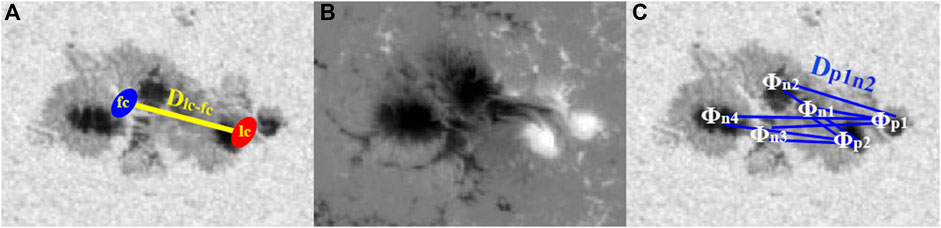
FIGURE 1. Figures illustrating the determination of the $S_{l-f}$ and $G_S$ morphological parameters. Panel (A) demonstrates, for $S_{l-f}$, how the distance $D_{lc-fc}$ is taken between the area-weighted centers (therefore the index c) of the spots of leading l and following f polarities. Panel (B) is the corresponding magnetogram of the continuum image of AR 11775, which were taken at 00:59 on 20 June 2013. Panel (C) present how the $G_S$ parameter is calculated. $\text{Φ}$ is the magnetic flux in a positive p or negative n umbra. D is the distance between two opposite-polarity umbrae.

The $S_{l-f}$ and $G_S$ can be determined from the moment of first available observation of sunspot groups, because the applied umbrae data are suitably corrected for geometrical foreshortening in the SOHO/MDI-Debrecen Data (SDD³) and the SDO/HMI—Debrecen Data (HMIDD⁴) catalogues (Baranyi et al., 2016). Furthermore, these two morphological parameters were shown to be potential indicators for upcoming flares on a smaller number of typical test cases (Korsós and Erdélyi, 2016). The test cases included 116 ARs, which were selected from SDD. Their selection was based on that about a third of the ARs produced only B- and C-class flares, another third produced M-class flares, and the remaining third produced X-class flares. For the statistical analysis, the considered values of $S_{l-f}$ and $G_S$ were determined 24, 48, and 72 hr before flare onset to test the conditional flare probability (CFP) of these two parameters. The CFPs were calculated as empirical probabilities, which measure the studied flare intensities and adequate recordings of the happening of events.

Korsós and Erdélyi (2016) found that if $S_{l-f}\le 1$ for a flaring AR then the CFP of the expected largest intensity flare being X-class is over at least 70%. If $1\le S_{l-f}\le 3$ the CFP is more than 45% for the largest-intensity flare(s) to be the M-class, and, if $3\le S_{l-f}\le 13$ there is larger than 60% CFP that C-class flare(s) may occurs within a 48-hr interval. Next, Korsós and Erdélyi (2016) found also that from analysing $G_S$ independently for determining the associated CFPs: if $7.5\le \log \left(G_S\right)$ then there is at least 70% chance for the strongest energy release to be X-class; if $6.5\le \log \left(G_S\right)\le 7.5$ then there is $\sim 45\%$ CFP that M-class could be the highest-intensity flares; finally, if $5.5\le \log \left(G_S\right)\le 6.5$, then it is very likely that C-class flare(s) may be the main intensity flares in the coming 48 h. ARs are unlikely to produce X-class flare(s) if $13\le S_{l-f}$ and $\log \left(G_S\right)\le 5.5$.

3 Data and Data Preparation

In this study, we further explore test and validate, the joint prediction capabilities of the $S_{l-f}$ and $G_S$ morphological parameters. The analysis is based on the binary logistic regression algorithm, using the Scikit-Learn module in Python (Pedregosa et al., 2011). The adopted ML technique requires appropriate historical datasets for training. Logistic regression is one of simplest and widely-used ML algorithms for two-class classification. Logistic regression is a special case of linear regression where the target variable is dichotomous in nature. Dichotomous means that there are only two possible classes, e.g., yes/no or true/false. Logistic regression also predicts the probability of occurrence of a binary event utilising a logit function.

Four training sets were constructed to enforce consistency in time and test robustness, each one corresponding to 6-, 12-, 18- and 24-hr forecast issuing time interval, because within a day the forecast reliability becomes more pronounced. The study takes as a reference the time of the largest flare event for each AR. For each issuing time interval, we consider the calculated $S_{l-f}$ or $G_S$ values of an AR before this reference time, as input data for the logistic regression. This framework allows us to quantify the prediction capabilities of the two morphological parameters.

Similarly to Korsós and Erdélyi (2016), this study uses information on around 1,000 ARs extracted from the Debrecen Sunspot Data Catalogue between 1996 and 2015 (Baranyi et al., 2016). The catalogue contains information including centroid position in various coordinate systems, area, and magnetic field of sunspots and sunspot groups. Derived from spacecraft observations, the catalogue has entries at each 1 hr for SDD⁵, and 1.5 hr for HMIDD⁶. The GOES⁷ flare catalogue is used for information on the largest-intensity flare eruption of each AR.

For each issuing time interval, two thirds of the ARs were randomly extracted to create a training set. These ARs are labeled as true(1) and false(0) events, under two different binary classification definition models:

• 1st model: When the largest intensity flare of an AR is M- or X-class then this case is classified as true(1), otherwise B- or C-class flares are false(0).

• 2nd model: Based on the results of Korsós and Erdélyi (2016), an event is true(1) if an AR is host to a M/X-class flare, satisfying $3\le S_{l-f}$, and $6.5\le \log \left(G_S\right)$. Or, an event is true(1) if an AR was host to a B/C-class flare, satisfying $S_{l-f}>3$, and $\log \left(G_S\right)<6.5$. Otherwise the cases are all labeled false(0).

The two different classification models were chosen to study whether the two morphological parameters perform better, either with or without (2nd or 1st model) thresholds. Often, a well-chosen threshold adjustment(s) could improve prediction capabilities of a method, as a warning level or as a warning sign. Furthermore, in the case of both model approaches as described above, the set of $S_{l-f}$ and $G_S$ values associated with the remaining 1/3 ARs are not labeled and are provided as a test set only for the logistic regression algorithm training. In this manner, there is no overlap between training and testing. To ensure robustness of the results, we replicated 100 times the training and test datasets for 6/12/18 and 24-hr issuing time intervals, like e.g., Campi et al. (2019).

4 Analysis

Solar flare prediction is affected by strong class imbalances, in that there are far more negative examples (labeled as N) than positive ones (labeled as P.) Therefore, we apply different metrics to measure the performance of the 1st and 2nd models. The performances of the two binary classifiers can be characterised by confusion matrixes in Figures 2, 3. Those confusion matrixes summarise the True Positive (TP), True Negative (TN), False Positive (FP), and False Negative (FN) predictions, we adopt different metrics to quantify the impact performance of the $S_{l-f}$ and $G_S$ parameters in the case of both model approaches (1st and 2nd). The applied metrics are summarised in Table 1 for 6-, 12-, 18- and 24-hr forecast issuing times, and are:

• Accuracy is the ratio of true positives plus true negatives over all events, or how often the TRUE prediction is correct: (TP + TN)/(P + N)

• Recall, also called the true positive rate or sensitivity, measures the proportion of actual positives that are correctly identified: TP/P

• Specificity, also called the true negative rate, measures the proportion of actual negatives that are correctly identified: TN/N

• Precision, also called positive predictive value. This is the ratio of true positives over all positive predictions: TP/(TP + FP).

• Negative predictive value (NPV) is the ratio of true negatives over all negative predictions: TN/(TN + FN).

• F1 score is the harmonic mean between sensitivity (or recall) and precision (or). It tells us how precise our two classifiers are, as well as how robust these are. A greater F1 score means that the performance of our model is better. Mathematically, F1 can be expressed as: 2 (1/Recall + 1/Precision)

• True Skill Statistic (TSS) is widely used to test the performance of forecasts (McBride and Ebert, 2000). TSS will be the preferred performance metric when comparing results of the 1st and 2nd model approaches with different N/P ratios because this metric is independent from the imbalance ratio (Woodcock, 1976; Bloomfield et al., 2012). TSS takes into account both omission and commission errors. The TSS parameter is similar to Cohen’s kappa approach (Shao and Halpin, 1995), and compares the predictions against the result of random guesses. TSS ranges from −1 to +1, where +1 indicates perfect agreement. The zero or less value indicates that a performance no better than random (Landis and Koch, 1977). TSS = TP/P−FP/N = Recall + Specificity-1

FIGURE 2

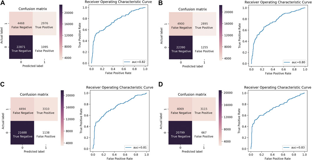
FIGURE 2. The result of the binary logistic regression of the 1^st model with 6-, 12-, 18-, and 24-hr forecast issuing times for panels (A), (B), (C), and (D) respectively. The right side of each panel presents the corresponding Receiver Operating Characteristic (ROC) curves.

FIGURE 3

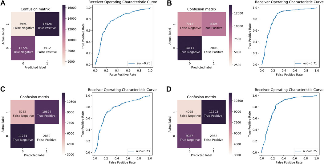
FIGURE 3. Same as Figure 2, but in the case of the 2^nd model.

TABLE 1

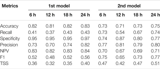
TABLE 1. Flare prediction capabilities with six metrics in the case of the two model approaches i.e., for 1st model and 2nd model.

These seven metric parameters are plotted as a function of forecast issuing times in Figure 4, where the blue/red lines stand for the 1st/2nd model. Based on the values of Table 1 and Figure 4, the two models have high accuracy for all forecast issuing times. In both models, the best accuracy is gained by the 24-hr prediction window. We emphasise that the accuracy is a meaningful measure only if the values of FP and FN would be similar in the confusion matrices of Figures 2, 3. For dissimilar values, the other metrics must be considered in evaluating the prediction performance of the two models.

FIGURE 4

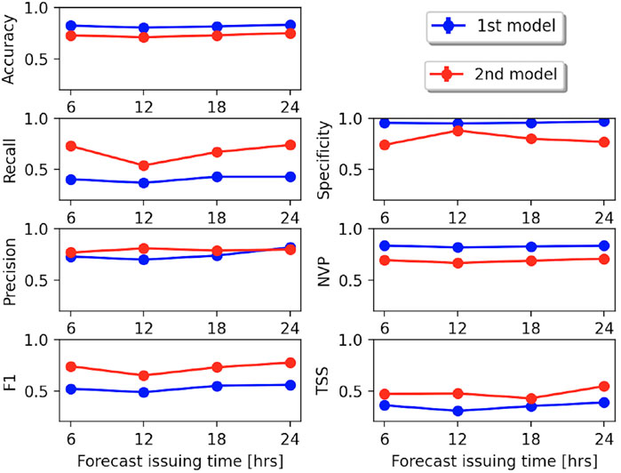
FIGURE 4. The evolution of selected metrics as a function of forecast issuing times for the 1st (blue) and 2nd (red) model.

Next, we focus on the recall and specificity metrics, which show the probability whether a model captures the correct classification during all four intervals. The values of the specificity metric show that the two models are capable to correctly classify TN cases during all four intervals, especially in the case of the 1st model, which is greater than 90%. Based on recall values, the TP classification of the 2nd model is 20% more accurate than the 1st model for 6/12/18/24-hr forecast issuing times.

However, when the two models classify a new AR, then we do not know the true outcome until after an event. Therefore, we are likely to be more interested in the question what is the probability of a true decision of the two models. This is measured by precision and NPV metrics. For the 1st model, the precision of the 24-hr prediction time is $\sim 10\%$ better than the other issuing time intervals, while the NPV values are $\sim 80\%$ in the case of four issuing time. The precision and NPV values of the 2nd model are almost the same over all four prediction windows. Based on precision and NPV metrics, the 2nd model predict a TP event with higher probability than the 1st model, while the 1st model is better with the case of TN event. This is because the 2nd model discards some X- and M-class flares which do not satisfy the threshold conditions. Despite this, the 2nd model still could fairly predict a TN event with about 70% probability.

The F1 and TSS metrics show that the 2nd model performs better than the 1st in the case of all of the prediction windows. This is an important aspect because the F1 and TSS are the most reliable scores in the presence of class imbalance. Intuitively, the F1 score is not as easy to understand as that of the accuracy, but it is usually more useful than accuracy, especially in our case, where we have an uneven class distribution. Namely, 77% of the F1 score shows that the 24-hr flare prediction window is the most efficient in the case of the 2nd model approach. Furthermore, the above 0.4 values of TSS score of the 2nd model show that this method is a good prediction scheme, and, the defined accuracy values of the 2nd model can be considered as correct.

We also use Receiver Operating Characteristic Curves (ROCs) to evaluated the results of the binary logistic regression method for both models. In the ROC plots in Figures 2, 3, the sensitivity (the proportion of true positive results) is shown on the y-axis, ranging from 0 to 1 (0–100%). The specificity (the proportion of false positive results) is plotted on the x-axis, also ranging from 0 to 1 (0–100%). The area under the curve (AUC) is a measure of the test’s performance at distinguishing positive and negative classes. In Figures 2, 3, AUCs are above 0.7, or a capability to distinguish between positive class and negative class with more than 70% likelihood over the 6-, 12-, 18- and 24-hr prediction time windows. From Figure 2, the 1st model shows similar AUC values during the four prediction windows. In the case of the 2nd model, the predicting probabilities are also similar based on the AUC values of Figure 3. On further note that the predicting probabilities of the 2nd model are 10% less than the 1st one, based on AUC values during the four prediction windows.

5 Conclusion

Korsós and Erdélyi (2016) introduced the separation parameter $S_{l-f}$ and the sum of the horizontal magnetic gradient $G_S$ as potential indirect indicators of the measure of non-potentiality of the magnetic fields of solar active regions. They also proposed these two morphological parameters as potential new prediction proxy indicators complementing the traditional Zürich, McIntosh or Mount Wilson classification schemes.

In this work, a binary logistic regression machine learning approach is used to test and validate the flare prediction capability of the $G_S$ and $S_{l-f}$ morphological parameters. Two binary classification schemes are used. One scheme is based on a simple approach while implementing solely flare intensity, the second approach is a more sophisticated model based on both flare intensity and threshold values of the morphological parameters. This experimental approach is applied to a large set of ∼1,000 ARs, with 100 repeats the datasets, over different forecast issuing time intervals of 6-, 12-, 18-, and 24-hr. Analysis of various performance metrics shows the following:

• The morphological parameters give more than 70% flare prediction accuracy, based on logistical regression analysis. This result supports the findings of Kontogiannis et al. (2018) and (Campi et al., 2019), who conclude that the $G_S$ parameter has potential as an efficient predictor.

• Based on the F1 scores and the True Skill Statistic metrics, the joint flare prediction efficiency of the $S_{l-f}$ and $G_S$ parameters is improved when the previously identified threshold values by Korsós and Erdélyi (2016) were also imposed. However, the 2nd model discards some X- and M-class flares which do not satisfy the threshold conditions. Despite of it, the 2nd model still could predict/classify an upcoming event with at least 70% probability, based on the precision and NPV metrics.

• The best flare prediction capability of the two parameters is available with 24-hr forecast issuing time. This latter means that the $S_{l-f}$ and $G_S$ parameters with their thresholds are capable to predict an upcoming flare with 75% accuracy a day before flare occurrence.

• However, not just the 24 hrs prediction window has good metric scores, but also the ones with 6/12 and 18 hrs. This means that the $S_{l-f}$ and $G_S$ are together applicable for prediction purpose in a short- and long-term one.

• The limitation of this study is that the applied data are extracted from a given sunspot database. Therefore, an other ML method (e.g., Convolutional Neural Network) that is trained on the same SDO/HMI intensity and magnetogram data, may assess further parameters to increase the predictive capability of the two morphological parameters.

We are aware that the two tested models are not perfect and so a natural question to ask is: how can we improve further them? In the future, we intend to further explore the application of these two warning parameters both from machine learning and physics perspectives: 1) fine tune the threshold conditions of 2nd model, 2) extend the application of the $S_{l-f}$ and $G_S$ parameters at different solar atmosphere heights, 3) train the employed machine learning model at different atmospheric heights for an even more accurate estimation of flare event time and flare event intensity, and 4) identify an optimal height range giving the earliest possible flare prediction, similar to the concept described by Korsos et al. (2020).

Data Availability Statement

Publicly available datasets were analyzed in this study. This data can be found here: http://fenyi.solarobs.csfk.mta.hu/ftp/pub/SDO/data/. http://fenyi.solarobs.csfk.mta.hu/ftp/pub/SDD/data/

Author Contributions

MK, RE, JL, and HM contributed to the conception and design of the study. MK performed the statistical analysis and wrote the first draft of the manuscript. All authors contributed to manuscript revision, read, and approved the submitted version.

Funding

MK and HM are grateful to the Science and Technology Facilities Council (STFC), (United Kingdom, Aberystwyth University, grant number ST/S000518/1), for the support received while carrying out this research. RE is grateful to STFC (United Kingdom, grant number ST/M000826/1) and EU H2020 (SOLARNET, grant number 158538). RE also acknowledges support from the Chinese Academy of Sciences President’s International Fellowship Initiative (PIFI, grant number 2019VMA0052) and The Royal Society (grant nr IE161153). JL acknowledges the support from STFC under grant No. ST/P000304/1.

Conflict of Interest

The authors declare that the research was conducted in the absence of any commercial or financial relationships that could be construed as a potential conflict of interest.

Acknowledgments

The authors are grateful to the Referees for constructive comments and recommendations which helped to improve the readability and quality of the paper.

Footnotes

¹http://hesperia.gsfc.nasa.gov/goes/goes_event_listings/

²http://flarecast.eu

³http://fenyi.solarobs.csfk.mta.hu/en/databases/SOHO/

⁴http://fenyi.solarobs.csfk.mta.hu/en/databases/SDO/

⁵http://fenyi.solarobs.csfk.mta.hu/en/databases/SOHO/

⁶http://fenyi.solarobs.csfk.mta.hu/en/databases/SDO/

⁷https://www.ngdc.noaa.gov/stp/space-weather/solar-data/solar-features/solar-flares/x-rays/goes/xrs/

References

Ahmed, O. W., Qahwaji, R., Colak, T., Dudok De Wit, T., and Ipson, S. (2010). A new technique for the calculation and 3D visualisation of magnetic complexities on solar satellite images. Vis. Comput. 26, 385–395. doi:10.1007/s00371-010-0418-1

CrossRef Full Text | Google Scholar

Ahmed, O. W., Qahwaji, R., Colak, T., Higgins, P. A., Gallagher, P. T., and Bloomfield, D. S. (2013). Solar flare prediction using advanced feature extraction, machine learning, and feature selection. Sol. Phys. 283, 157–175. doi:10.1007/s11207-011-9896-1

CrossRef Full Text | Google Scholar

Al-Ghraibah, A., Boucheron, L. E., and McAteer, R. T. J. (2015). An automated classification approach to ranking photospheric proxies of magnetic energy build-up. Astron. AstroPhys. 579, A64. doi:10.1051/0004-6361/201525978

CrossRef Full Text | Google Scholar

Baranyi, T., Győri, L., and Ludmány, A. (2016). On-line tools for solar data compiled at the debrecen observatory and their extensions with the Greenwich sunspot data. Sol. Phys. 291, 3081–3102. doi:10.1007/s11207-016-0930-1

CrossRef Full Text | Google Scholar

Barnes, G., Leka, K. D., Schrijver, C. J., Colak, T., Qahwaji, R., Ashamari, O. W., et al. (2016). A comparison of flare forecasting methods. I. Results from the all-clear workshop. Astrophys. J. 829, 89. doi:10.3847/0004-637X/829/2/89

CrossRef Full Text | Google Scholar

Benz, A. O. (2008). Flare observations. Living Rev. Sol. Phys. 5, 1. doi:10.12942/lrsp-2008-1

PubMed Abstract | CrossRef Full Text | Google Scholar

Bloomfield, D. S., Higgins, P. A., McAteer, R. T. J., and Gallagher, P. T. (2012). Toward reliable benchmarking of solar flare forecasting methods. Astrophys. J. Lett. 747, L41. doi:10.1088/2041-8205/747/2/L41

CrossRef Full Text | Google Scholar

Bobra, M. G., and Couvidat, S. (2015). Solar flare prediction using SDO/HMI vector magnetic field data with a machine-learning algorithm. Astrophys. J. 798, 135. doi:10.1088/0004-637X/798/2/135

CrossRef Full Text | Google Scholar

Boucheron, L. E., Al-Ghraibah, A., and McAteer, R. T. J. (2015). Prediction of solar flare size and time-to-flare using support vector machine regression. Astrophys. J. 812, 51. doi:10.1088/0004-637X/812/1/51

CrossRef Full Text | Google Scholar

Campi, C., Benvenuto, F., Massone, A. M., Bloomfield, D. S., Georgoulis, M. K., and Piana, M. (2019). Feature ranking of active region source properties in solar flare forecasting and the uncompromised stochasticity of flare occurrence. Astrophys. J. 883, 150. doi:10.3847/1538-4357/ab3c26

CrossRef Full Text | Google Scholar

Camporeale, E. (2019). The challenge of machine learning in space weather: nowcasting and forecasting. Space Weather 17, 1166–1207. doi:10.1029/2018SW002061

CrossRef Full Text | Google Scholar

Domijan, K., Bloomfield, D. S., and Pitié, F. (2019). Solar flare forecasting from magnetic feature properties generated by the solar monitor active region tracker. Sol. Phys. 294, 6. doi:10.1007/s11207-018-1392-4

CrossRef Full Text | Google Scholar

Gallagher, P. T., Moon, Y.-J., and Wang, H. (2002). Active-region monitoring and flare forecasting I. Data processing and first results. Sol. Phys. 209, 171–183. doi:10.1023/A:1020950221179

CrossRef Full Text | Google Scholar

Georgoulis, M. K., and Rust, D. M. (2007). Quantitative forecasting of major solar flares. Astrophys. J. Lett. 661, L109–L112. doi:10.1086/518718

CrossRef Full Text | Google Scholar

Hale, G. E., Ellerman, F., Nicholson, S. B., and Joy, A. H. (1919). The magnetic polarity of sun-spots. Astrophys. J. 49, 153. doi:10.1086/142452

CrossRef Full Text | Google Scholar

Hayes, L. A., Gallagher, P. T., McCauley, J., Dennis, B. R., Ireland, J., and Inglis, A. (2017). Pulsations in the Earth’s lower ionosphere synchronized with solar flare emission. J. Geophys. Res. 122, 9841–9847. doi:10.1002/2017JA024647

CrossRef Full Text | Google Scholar

Ireland, J., Young, C. A., McAteer, R. T. J., Whelan, C., Hewett, R. J., and Gallagher, P. T. (2008). Multiresolution analysis of active region magnetic structure and its correlation with the Mount Wilson classification and flaring activity. Sol. Phys. 252, 121–137. doi:10.1007/s11207-008-9233-5

CrossRef Full Text | Google Scholar

Kiepenheuer, K. O. (1953). Solar activity. Chicago, IL: The University of Chicago Press, 322.

Google Scholar

Kontogiannis, I., Georgoulis, M. K., Park, S.-H., and Guerra, J. A. (2017). Non-neutralized electric currents in solar active regions and flare productivity. Sol. Phys. 292, 159. doi:10.1007/s11207-017-1185-1

CrossRef Full Text | Google Scholar

Kontogiannis, I., Georgoulis, M. K., Park, S.-H., and Guerra, J. A. (2018). Testing and improving a set of morphological predictors of flaring activity. Sol. Phys. 293, 96. doi:10.1007/s11207-018-1317-2

CrossRef Full Text | Google Scholar

Korsós, M. B., and Erdélyi, R. (2016). On the state of a solar active region before flares and CMEs. Astrophys. J. 823, 153. doi:10.3847/0004-637X/823/2/153

CrossRef Full Text | Google Scholar

Korsós, M. B., Baranyi, T., and Ludmány, A. (2014). Pre-flare dynamics of sunspot groups. Astrophys. J 789, 107. doi:10.1088/0004-637X/789/2/107

CrossRef Full Text | Google Scholar

Korsos, M. B., Georgoulis, M. K., Gyenge, N., Bisoi, S. K., Yu, S., Poedts, S., et al. (2020). Solar flare prediction using magnetic field diagnostics above the photosphere. Astrophys. J. 896 (2), 119. doi:10.3847/1538-4357/ab8fa2

CrossRef Full Text | Google Scholar

Künzel, H. (1960). Die Flare-Häufigkeit in Fleckengruppen unterschiedlicher Klasse und magnetischer Struktur. Astron. Nachr. 285, 271. doi:10.1002/asna.19592850516

CrossRef Full Text | Google Scholar

Landis, J. R., and Koch, G. G. (1977). The measurement of observer agreement for categorical data. Biometrics 33, 159–174. doi:10.2307/2529310

PubMed Abstract | CrossRef Full Text | Google Scholar

Leka, K. D., Barnes, G., and Wagner, E. (2018). The NWRA classification infrastructure: description and extension to the discriminant analysis flare forecasting system (DAFFS). J. Space Weather and Space Clim. 8, A25. doi:10.1051/swsc/2018004

CrossRef Full Text | Google Scholar

Leka, K. D., Park, S.-H., Kusano, K., Andries, J., Barnes, G., Bingham, S., et al. (2019a). A comparison of flare forecasting methods. II. Benchmarks, metrics, and performance results for operational solar flare forecasting systems. Astrophys. J. 243, 36. doi:10.3847/1538-4365/ab2e12

CrossRef Full Text | Google Scholar

Leka, K. D., Park, S.-H., Kusano, K., Andries, J., Barnes, G., Bingham, S., et al. (2019b). A comparison of flare forecasting methods. III. Systematic behaviors of operational solar flare forecasting systems. Astrophys. J. 881, 101. doi:10.3847/1538-4357/ab2e11

CrossRef Full Text | Google Scholar

Liu, C., Deng, N., Wang, J., and Wang, H. (2017). “Predicting solar flares using SDO/HMI vector magnetic data product and random forest algorithm,” Astrophys. J. 843 (2), 104. doi:10.3847/1538-4357/aa789b

CrossRef Full Text | Google Scholar

McBride, J. L., and Ebert, E. E. (2000). Verification of quantitative precipitation forecasts from operational numerical weather prediction models over Australia. Weather Forecast 15, 103–121. doi:10.1175/1520-0434(2000)015<0103:VOQPFF>2.0.CO;2

CrossRef Full Text | Google Scholar

McIntosh, P. S. (1990). The classification of sunspot groups. Sol. Phys. 125, 251–267. doi:10.1007/BF00158405

CrossRef Full Text | Google Scholar

Nishizuka, N., Sugiura, K., Kubo, Y., Den, M., and Ishii, M. (2018). Deep flare net (DeFN) model for solar flare prediction. Astrophys. J. 858, 113. doi:10.3847/1538-4357/aab9a7

CrossRef Full Text | Google Scholar

Park, S.-H., Leka, K. D., Kusano, K., Andries, J., Barnes, G., Bingham, S., et al. (2020). A comparison of flare forecasting methods. IV. Evaluating consecutive-day forecasting patterns. Astrophys. J. 890, 124. doi:10.3847/1538-4357/ab65f0

CrossRef Full Text | Google Scholar

Pedregosa, F., Varoquaux, G., Gramfort, A., Michel, V., Thirion, B., Grisel, O., et al. (2011). Scikit-learn: machine learning in Python. J. Mach. Learn. Res. 12, 2825–2830. doi:10.1016/j.patcog.2011.04.006

CrossRef Full Text | Google Scholar

Schrijver, C. J. (2016). The nonpotentiality of coronae of solar active regions, the dynamics of the surface magnetic field, and the potential for large flares. Astrophys. J. 820, 103. doi:10.3847/0004-637X/820/2/103

CrossRef Full Text | Google Scholar

Shao, G., and Halpin, P. N. (1995). Climatic controls of eastern north american coastal tree and shrub distributions. J. Biogeogr. 22, 1083–1089. doi:10.2307/2845837

CrossRef Full Text | Google Scholar

Song, H., Tan, C., Jing, J., Wang, H., Yurchyshyn, V., and Abramenko, V. (2009). Statistical assessment of photospheric magnetic features in imminent solar flare predictions. Sol. Phys. 254, 101–125. doi:10.1007/s11207-008-9288-3

CrossRef Full Text | Google Scholar

Tziotziou, K., Sandberg, I., Anastasiadis, A., Daglis, I. A., and Nieminen, P. (2010). Using a new set of space-borne particle monitors to investigate solar-terrestrial relations. Astron. AstroPhys. 514, A21. doi:10.1051/0004-6361/200912928

CrossRef Full Text | Google Scholar

Waldmeier, M. (1938). Chromosphärische eruptionen. I. Mit 6 abbildungen. Z. AstroPhys. 16, 276.

Google Scholar

Woodcock, F. (1976). The evaluation of yes/no forecasts for scientific and administrative purposes. Mon. Weather Rev. 104, 1209. doi:10.1175/1520-0493(1976)104<1209:TEOYFF>2.0.CO;2

CrossRef Full Text | Google Scholar

Yu, D., Huang, X., Wang, H., and Cui, Y. (2009). Short-term solar flare prediction using a sequential supervised learning method. Sol. Phys. 255, 91–105. doi:10.1007/s11207-009-9318-9

CrossRef Full Text | Google Scholar