Structure of the Solar Atmosphere: A Radio Perspective

1. Introduction

By definition, the atmosphere of a star is the region from which photons can escape and reach the observer. Photons are not our only source of information for the Sun; important information can also be obtained from particles originating on the Sun and reaching the vicinity of the Earth, both in the form of the quasi-steady flow of the solar wind and during energetic events. The magnetic field carried by the solar wind plasma is also an important carrier of information. Last but not least, neutrinos and global oscillations have provided us with a wealth of information on the solar interior. Still, the bulk of what we know about the Sun comes from photons, thus in this review we will restrict ourselves to the results obtained from the analysis of the solar electromagnetic emission, in an attempt to compile a concise, but still comprehensive picture of the structure of the solar atmosphere; we will also try to give a historical perspective, as far as possible. More details can be found in a number of monographs on the Sun (Kuiper, 1953; Zirin, 1966, 1988; Priest, 1987, 2014; Durrant, 1988; Foukal, 2004; Stix, 2004; Aschwanden, 2004; Engvold et al., 2019) and on solar radio astronomy (Kundu, 1965; Zheleznyakov, 1970; Krueger, 1979; McLean and Labrum, 1985; Gary and Keller, 2004). There are also reviews on the Quiet Sun radio emission that the reader might be interested in (Alissandrakis, 1994; Gary, 1996; Alissandrakis and Einaudi, 1997; Lantos, 1999; Shibasaki, 1999; Keller and Krucker, 2004 and Shibasaki et al., 2011). Also of interest to the readers will be the reviews on Coherent Emission Mechanisms (Nindos, 2020) and on Radio Measurements of the Magnetic field (Alissandrakis and Gary, 2020), included in this special research topic collection.

As a rule, the term structure refers to the description of physical parameters as a function of position (in three dimensions) and time. As far as the time scale is concerned, solar phenomena are divided in three groups: the Quiet Sun (QS), the slowly varying component and the sporadic component. This grouping also reflects the energy associated with the phenomena, with the sporadic emission being the most energetic. Here we will not discuss sporadic phenomena, but we will only consider the Quiet Sun and, briefly, the slowly varying component that form the background for the more energetic phenomena.

It is important to stress that, as the solar emission extends over a wide spectral range, from γ-rays to radio waves, no single spectral window can provide complete information on solar phenomena. Yet, for reasons that have to do with the instrumentation and the effects of the earth's atmosphere, astronomical observations refer to particular spectral windows. Each spectral window offers unique information, radio being no exception. Addressing an audience of solar radio astronomers, we will try to emphasize what this spectral range has offered to our understanding of the Sun and to integrate radio data with data from other spectral ranges.

Although this chapter is about the Sun's atmosphere, we will start with a brief section on its interior, which plays the role of the source for all atmospheric phenomena. We will continue with a discussion of the radial structure of the solar atmosphere and then with its horizontal structure. We will then pass to active regions and we will finish with a discussion of the heating problem.

2. From the core to the solar atmosphere

Until a few decades ago, we had no direct information about the interior of the Sun; what we knew was based on the theory of stellar structure, which produced the so called standard model of the solar interior. The most important conclusion, apart from the fact that conditions in the solar core are appropriate for the fusion of hydrogen to helium through the proton-proton cycle, is that the interior of the Sun is radiative up to ~ 0.71R_⊙, where convection starts and operates up to the subphotospheric layers. The convection zone has huge implications on the solar dynamo (Ossendrijver, 2003; Charbonneau, 2010), producing the magnetic field observed in the atmospheric layers and governing their structure.

The detection of neutrinos produced by nuclear fusion reactions in the solar core opened up a new area of research (Davis, 2003). However, it turned out that neutrino astronomy gave us more information about the properties of neutrinos such as neutrino oscillations (Ahmad et al., 2002), rather than the solar interior. Real observational information about the interior of the Sun came with helioseismology (see reviews by Christensen-Dalsgaard, 2002, Basu, 2016, García and Ballot, 2019).

Helioseismological spectral data are as rich in spectral lines as the optical solar spectrum or even richer, and their inversion allows us to measure quantities such as the speed of sound and the speed of rotation in the solar interior. The most impressive results are the excellent agreement with the standard model (see Figure 6 in Basu et al., 1997) and the rigid rotation of the solar interior (see Figure 18 in Christensen-Dalsgaard, 2002) below the convection zone.

Acoustic (p) modes cannot probe the deep solar interior; g modes, for which gravity (buoyancy) is the restoring force, are much better in this respect (see review by Appourchaux et al., 2010). However, gravity waves cannot propagate in a convectively unstable medium, such as the convection zone; they are evanescent there and are expected to come out in the photosphere with a much reduced, amplitude. A recent report on the detection of g-modes (Fossat et al., 2017) has been contested by Appourchaux and Corbard (2019).

With the advent of time-distance seismology, we have also been able to map the structure of the solar interior in the sub-photospheric layers (see review by Gizon et al., 2010; also Kosovichev, 2011). Impressive results have been obtained on the subphotospheric structure of sunspots (Gizon et al., 2009; Zhao et al., 2010) and supergranular flows (Jackiewicz et al., 2008). We can even detect active regions on the far side of the solar disk (see the recent article by Zhao et al., 2019), with data routinely available at http://jsoc.stanford.edu/data/farside/.

3. Atmospheric structure

3.1. Elementary Physics of the Solar Atmosphere

Part of energy radiated by the Sun reaches the earth and it can be measured. From the value of the solar constant (the energy per unit area per unit time at 1 AU), together with the solar radius and the sun-earth distance, the effective temperature of the visible layer of the solar atmosphere (the photosphere) can be computed. Its value of 5,800 K gives us a measure of the photospheric temperature, and this is very important information.

Let us note further that in visible light the Sun appears as a disk with a sharp limb. From this elementary remark we can infer that the photospheric density decreases very fast with height. Let us start from the equation of hydrostatic equilibrium,

$\begin{array}{ll}\frac{dP}{dz}=-g\rho & (1)\end{array}$

where P is the pressure, g the gravity (assumed constant), ρ is the density, and z the height. We can further express the pressure in terms of the density, using the equation of state,

$\begin{array}{ll}P=N{k}_{B}T=\frac{\rho }{{\mu }_{mol}{m}_H}{k}_{B}T& (2)\end{array}$

where N is the number density of particles, μ_mol is the mean molecular weight (= 1 for an atmosphere of neutral Hydrogen, 0.5 for fully ionized Hydrogen, 0.61 for 10% Helium), m_H the hydrogen mass, k_B the Boltzmann constant and T the temperature. Integrating (1), under the (crude) isothermal approximation, we obtain:

$\begin{array}{ll}\rho ={\rho }_o{e}^{-z/H}& (3)\end{array}$

where ρ_o is the density at z = 0 and

$\begin{array}{ll}H=\frac{kT}{g{\mu }_{mol}{m}_H}& (4)\end{array}$

is the isothermal scale height. Expressions similar to (3) hold for the pressure and for the number density. For the effective temperature of the photosphere, the scale height is a mere 175 km, i.e., just 0.0025 R_⊙, which tells us that the photosphere is very thin and, at the same time, explains why the optical limb is so sharp.

Another well-known fact is that, during total eclipses of the Sun and at the time that the moon has covered completely the photosphere, a bright red-colored crescent appears, the chromosphere. Its extent is certainly greater than that of the photosphere and this, following the argument about the scale height, implies that it has a higher temperature; indeed, more precise measurements give chromospheric temperatures of 10 to 20 × 10³ K. The fact that it is much fainter than the photosphere, indicates that it has also a much lower density. Finally, much more extended, faint and diffuse than the chromosphere is the corona, which appears when the chromosphere has been covered by the moon. It has a scale height that indicates million-degree temperature and, of course, is much less dense than the chromosphere. Last but not least, the huge temperature difference between the chromosphere and the corona (2 × 10⁴ to 10⁶ K) requires a chromosphere-corona Transition Region (TR) to bridge the two.

Thus, using simple physical arguments, we have discovered the principal layers of the solar atmosphere and we have come across a basic problem of solar physics: that of the heating of the chromosphere and the corona, which we will discuss further in section 7.

3.2. Extracting the Information

In order to go beyond the elementary arguments of the previous section, we have to know how the physical conditions influence the production and transport of photons. The electromagnetic radiation that comes to us is rich in information about the physical conditions in the region of its formation, such as the electron temperature, the electron density and pressure, the magnetic field, the velocity of flow, the abundance of elements etc. It is the astrophysicist's task to extract this information and the main tool for this is the theory of radiative transfer (Mihalas, 1970; Rutten, 2003). Without going into the details, let us remind the reader that the specific intensity, I_ν, observed at the frequency, ν, that reaches the observer from a stellar atmosphere is given by the formal solution of the transfer equation for a plane-parallel, semi-infinite atmosphere:

$\begin{array}{ll}{I}_{\nu }({\tau }_{\nu }=0,\mu )={\displaystyle {\int }_0^{\infty }}{S}_{\nu }{e}^{-{\tau }_{\nu }/\mu }d{\tau }_{\nu }/\mu & (5)\end{array}$

Here the integration is carried along the vertical (radial) direction, z, which forms an angle θ with the path of the radiation (i.e., with the line of sight, in the absence of refraction), hence the presence of μ = cos θ in (5), θ being the heliocentric angle; the position along the vertical is expressed in terms of the optical depth, τ_ν, which is related to the geometrical height, z, and the opacity of the material through:

$\begin{array}{ll}d{\tau }_{\nu }=-k_{\nu }\rho dz& (6)\end{array}$

where ρ is the density of the material and k_ν is the absorption coefficient. The minus sign is because the optical depth is measured from the observer to the star, while z is measured in the opposite direction. Furthermore, S_ν in (5) is the source function, which is the ratio of the coefficients of emission, j_ν, and absorption, k_ν,

$\begin{array}{ll}{S}_{\nu }=\frac{j_{\nu }}{k_{\nu }}& (7)\end{array}$

and expresses the emissivity of the material; it is equal to the Plank function, B_ν(T), under conditions of Local Thermodynamic Equilibrium (LTE).

From the very form of (5), we can see that the specific intensity carries information about all atmospheric layers and that the contribution of each layer is weighted by the local value of the source function and reduced by the absorption of overlying layers. It is easy to prove that, in first order, the observed specific intensity corresponds to the value of the source function at τ_ν = μ (Eddington-Barbier relation); thus at the center of the disk we see at τ_ν ≃ 1.

In practice, we can probe the atmosphere by two means. One is by varying μ, which can be done by measuring the variation of the specific intensity from the center of the solar disk (μ = 1) to the limb (μ = 0). It is easy to show that, if the temperature decreases with height, the intensity at the limb is lower than at the disk center (limb darkening); in the opposite case the limb is brighter. Figure 1, top row, shows three full disk solar images. Two of them, in the optical range, show limb darkening (more in the blue than in the red part of the spectrum), which proves that the temperature is decreasing with height in the region of formation of the radiation (photosphere); the third, in the microwave range, shows signs of limb brightening, which indicates that the temperature is rising above the photosphere, where the radiation is formed.

FIGURE 1

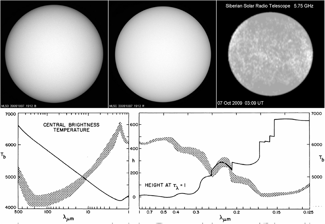
Figure 1. (Top) Solar images on October 7, 2009 in the blue part of the spectrum (left) in the red (middle) from the Mauna Loa Solar Observatory (MLSO) and at λ = 5.2 cm from the Siberian Solar Radio Telescope (SSRT); images selected by the author. (Bottom) Observed continuum brightness temperature at the center of the solar disk as a function of wavelength (shaded band) and the approximate height of formation of the radiation (black line); from Vernazza et al. (1976), © AAS, reproduced with permission.

The second method for probing the atmosphere is by varying the frequency of observation, which changes the opacity. As shown in the bottom row of Figure 1, this allows us to probe a height range of ~ 600 km, where the temperature ranges from ~ 4, 500 to ~ 6, 700 K, in the spectral range from sub-mm λ to the far ultraviolet.

It follows from the above discussion that, in principle, one could invert (5) and recover the information on the physical conditions. This is the basis for the computation of empirical atmospheric models (see Chapter 6.10 in Zirin, 1988). Things are not simple though, because of the complex dependence of the absorption coefficient on the physical conditions and due to departures from LTE in the upper solar atmosphere. The situation is better in the radio range, thanks to the Rayleigh-Jeans approximation to the Planck function and the fact that electrons, which are responsible for the thermal emission, are always in LTE. Under these circumstances, the solution of the transfer equation takes the form:

$\begin{array}{ll}{T}_b={\displaystyle {\int }_0^{\infty }}{T}_e{e}^{-{\tau }_{\nu }/\mu }d{\tau }_{\nu }/\mu & (8)\end{array}$

which links the electron temperature, T_e, to the observed brightness temperature, T_b, defined so that

$\begin{array}{ll}{I}_{\nu }=\frac{2k{T}_b}{{\lambda }^2}& (9)\end{array}$

We will finish the section by considering the emission of a homogeneous slab of material (cloud), overlying a background of specific intensity I_νo:

$\begin{array}{ll}{I}_{\nu }=I_{\nu o}{e}^{-{\tau }_{\nu }}+S_{\nu }(1-e^{-{\tau }_{\nu }})& (10)\end{array}$

or, for the radio range,

$\begin{array}{ll}{T}_b=T_{bo}{e}^{-{\tau }_{\nu }}+T_e(1-e^{-{\tau }_{\nu }})& (11)\end{array}$

An important consequence of these relations is that, if the slab is optically thick, a measurement of the brightness temperature gives us directly the value of the electron temperature (T_b ≃ T_e, for τ_ν >> 1). If, on the contrary, the slab is optically thin (τ_ν << 1) and there is no background emission, its brightness temperature is lower than its electron temperature:

$\begin{array}{ll}{T}_b=\tau T_e.& (12)\end{array}$

4. Radial structure of the solar atmosphere

In the previous section we implicitly assumed that solar parameters vary only in the radial direction. However, anyone who has seen solar images will agree that the Sun is extremely rich in structure in the non-radial direction (horizontal structure) and that inhomogeneities become more prominent as we move from the photosphere to the chromosphere and the corona. Moreover, as the spatial resolution of our instruments increases, we become more and more aware of the importance of horizontal structures.

Under these circumstances, it is rather surprising that one-dimensional models which, in addition to treating the physical parameters as a function of height only, also assume hydrostatic equilibrium, have any resemblance to the observations at all. The physical reason behind the success of such models is gravity, which produces a strong radial stratification in the solar atmosphere; as a consequence, the radial density gradient is much larger than the horizontal, at least in the lower atmospheric layers.

4.1. Empirical Models for the Low Atmosphere

There is a long tradition of 1-D empirical solar models. Early models did not extend beyond the chromosphere, stopping around $T_e\simeq 10^4$ K, which is too low for brightness computations beyond the cm radio wavelength range. Subsequent models went higher, with that of Fontenla et al. (2002) reaching 1.2 × 10⁶ K, in the upper TR. These models also developed further the multi-component approach, first introduced in Vernazza et al. (1981), to represent different quiet and active regions on the Sun. Note that multi-component models are not really 3-D, since radiative transfer in the horizontal direction is ignored. More details can be found in Shibasaki et al. (2011).

With the advent of fast numerical computations, a number of sophisticated tools, such as the bifrost radiative magnetohydrodynamics (rMHD) code (Gudiksen et al., 2011) and the STockholm inversion Code (STic, de la Cruz Rodríguez et al., 2019) have been developed for solar atmospheric modeling. Nevertheless, the classic models still provide a comprehensive picture of the solar atmosphere.

In order to compute brightness spectra at longer wavelengths, one has to add a coronal contribution. Zirin et al. (1991) found that their measurements, which extended up to 21 cm, could simply be reproduced by a two-component model: an optically thick chromosphere and an isothermal corona (see further discussion in section 4.3.2). Selhorst et al. (2005) used a hybrid model (combination of models for the photosphere, chromosphere, and corona) to reproduce the observed features in Nobeyama Radioheliograph (NoRH) images at 17 GHz. To obtain acceptable brightness temperature values and the observed solar radius, they had to include absorbing chromospheric structures, such as spicules (see section 5.3) into the model, as had been done in the past (e.g., Lantos and Kundu, 1972), in order to explain why the observed center-to-limb variation shows less brightening than the homogeneous models predict, or even shows darkening.

Solar observations with the Atacama Large mm and sub-mm Array (ALMA) are providing new information on the structure of the low atmosphere. Alissandrakis et al. (2017, 2020) used the center-to-limb variation of the brightness temperature from ALMA full-disk data at 1.25 and 3 mm and data from Bastian et al. (1993) at 0.85 mm to invert the transfer equation and obtained the electron temperature as a function of the optical depth (Figure 2). Their results were close (5% lower) to the predictions of the Fontenla et al. (1993) average QS model C.

FIGURE 2

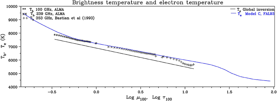
Figure 2. Observed brightness temperature in the mm-λ range, T_b as a function of the cosine of heliocentric angle, μ₁₀₀, reduced to 100 MHz (symbols). The same plot shows the computed electron temperature, T_e as a function of the optical depth, τ₁₀₀, (black line), again reduced to 100 GHz. The blue line gives T_e(τ₁₀₀) predicted by model C of Fontenla et al. (1993). Note that increasing τ corresponds to decreasing altitude in the atmosphere. Adapted from Alissandrakis et al. (2017), reproduced with permission © ESO.

4.2. Emission Measure and Differential Emission Measure

Several authors have used direct information from the EUV part of the spectrum to compute the radio brightness in the microwave range, which is reasonable since the radiation in both wavelength ranges is formed in the same atmospheric layers. In one approach the emission measure, EM, which is a measure of the electron density, N_e, along the line of sight, is used:

$\begin{array}{ll}EM={\displaystyle {\int }_0^L}{N}_e^{2}d\ell & (13)\end{array}$

This quantity appears both in the expression for the integrated intensity of EUV lines and the radio brightness temperature, provided that the emission is optically thin and the plasma isothermal (see Shibasaki et al., 2011 for details). This fact led to the well-known practice of using two EUV lines or X-ray continuum bands for an estimate of the plasma temperature and the emission measure. Zhang et al. (2001) used three EIT images, at 171, 195, and 284 Å, to derive the emission measure in a two-temperature model. They further computed the emission at 6 and 20 cm wavelengths, which they compared with their Very Large Array (VLA) observations. Although the model image looks very much like the observed, the computed brightness temperature was twice the observed at both wavelengths; at 6 cm the model gave ~ 170 × 10³ K vs. the observed ~ 85 × 10³ K, whereas at 20 cm the values were ~ 1.5 × 10⁶ K and ~ 0.8 × 10⁶ K respectively (see their Figure 4). They attributed the discrepancy to errors in the coronal abundances used to infer the radio flux from the EIT data.

The differential emission measure (DEM) is even better than the emission measure; it is defined as

$\begin{array}{ll}\phi (T_e)=N_e^2\frac{d\ell }{d{T}_e}& (14)\end{array}$

and represents the distribution of electron density over a temperature range, dropping the isothermal assumption. Obviously, one needs many EUV lines, formed over the appropriate temperature range, to make good use of the DEM.

Landi and Chiuderi Drago (2003) used the DEM values derived from UV and EUV spectral line intensities observed by SUMER and CDS, and showed that a TR model for the cell interior—excluding any network contribution—could give an agreement with the observed radio brightness temperatures (see section 5.2 for explanations of the network and the cell interior). In a subsequent work, (Landi and Chiuderi Drago, 2008), they showed that radio observations provide a much more reliable diagnostic tool for the determination of the DEM than UV and EUV lines at T < 30000 K, since the latter are optically thick. Moreover, they extended the DEM down to 5,600 K using the radio spectrum from 1.5 to 345 GHz, and obtained very good agreement with the radio data.

Useful as it may be, the DEM cannot be used to compute the emission in optically thick cases, in which case both T_e and N_e are required to integrate (8). Still, in a recent work, Alissandrakis et al. (2019) developed a method for the computation of the electron temperature and density along the line of sight from the DEM, under the assumptions of stratification and hydrostatic equilibrium and used it to compute the cm-λ emission from active regions.

4.3. Coronal and Transition Region Models

As we move from the microwave to the metric range, the height of formation of the radiation increases due to the increase of the absorption and, eventually, we reach the corona. This leads to an increase of the solar radius with wavelength (see, e.g., Figure 5 of Menezes and Valio, 2017), although this quantity is not the most accurate way to measure the formation height due to structures beyond the limb and other effects. Hence, in order to understand the radio emission at dm-λ and beyond, it is important to discuss the information obtained for the layers above the chromosphere from other spectral ranges.

4.3.1. Models From Optical Data

As mentioned already in section 3.1, the extent of the corona indicates a large scale height and a high temperature. Emission lines in the optical spectrum (the emission line or E-corona), also provide evidence for a hot corona. These lines, originally attributed to an unknown element (coronium), turned out to be due to forbidden transitions of highly ionized species, such as FeX (the red line at 6374 Å), FeXIV (the green line at 5303 Å) and CaXV (the yellow line at 5494 Å); they were identified thanks to the work of Grotrian (1939) and of Edlén (1943). The issue of their formation temperature was not settled, until dielectronic recombination was taken into account (for a vivid account see Chapters 6.3 and 7.3 in Zirin's 1966 book).

Due to the difficulties in the interpretation of the line emission, coronal models are based on the continuum white light corona, which is due to Thomson scattering of photospheric photons on the free electrons of the coronal plasma (van de Hulst, 1950). This emission is linearly polarized and constitutes the K corona (kontinuierlich); there is also unpolarized emission (the F corona), which is due to Rayleigh scattering of the Fraunhofer spectrum in dust and small particles between the Sun and the Earth.

Assuming spherical symmetry, a number of models have been produced (Allen, 1947; van de Hulst, 1950; Newkirk, 1961; Saito et al., 1970) from K corona data. In spite of the fact that the corona is highly inhomogeneous, some of them, namely the Newkirk (1961) and Saito et al. (1970) models, were quite successful in describing the coronal density and are still in use. They are very useful in modeling the radio emission and in estimating the height of metric burst sources. In such cases the emission is at the plasma frequency, f_p:

$\begin{array}{ll}{f}_p\left[\text{MHz}\right]=8.978\times 10^{-3}\sqrt{N_e\left[{\text{cm}}^{-3}\right]}& (15)\end{array}$

or the second harmonic; the height of the emission is then derived from the observed frequency and the density model.

The Newkirk model predicts a variation of the electron density, N_e, with the distance, r, from the center of the Sun that has the form:

$\begin{array}{ll}{N}_e=4.2\times 10^{4}10^{4.32R_{\text{⊙}}/r}=4.2\times 10^4{e}^{9.95R_{\text{⊙}}/r}\left[{\text{cm}}^{-3}\right]& (16)\end{array}$

where R_⊙ is the solar radius. This is hydrostatic, since the solution of the hydrostatic equilibrium equation (1) in spherical coordinates, taking into account the variation of gravity with height, is:

$\begin{array}{ll}{N}_e=N_{eo}{e}^{-\frac{R_{\text{⊙}}}{H_{\text{⊙}}}+\frac{R_{\text{⊙}}}{H_{\text{⊙}}}\frac{R_{\text{⊙}}}{r}}& (17)\end{array}$

where H_⊙ is the scale height at the base of the corona. A comparison with (16) gives,

$\begin{array}{ll}{N}_{eo}=8.8\times 10^8{\text{ cm}}^{-3}& (18)\end{array}$

$\begin{array}{ll}{H}_{\text{⊙}}=0.1005R_{\text{⊙}}=\mathrm{70\; 000}\text{ km}& (19)\end{array}$

this value of the scale height corresponds to a coronal temperature of T = 1.41 × 10⁶ K.

The Saito model allows for density variations with latitude, φ:

$\begin{array}{l}{N}_e=\frac{3.09\times 10^8(1-0.95\text{ sin }\phi )}{{(r/R_{\text{⊙}})}^{16}}+\frac{1.58\times 10^8(1-0.5\text{ sin }\phi )}{{(r/R_{\text{⊙}})}^6}\\ +\frac{0.0251\times 10^8(1-\sqrt{\text{ sin }\phi })}{{(r/R_{\text{⊙}})}^{2.5}}\left[{\text{cm}}^{-3}\right]& (20)\end{array}$

The Saito polar corona reflects coronal hole conditions, but coronal holes were not known at the time. The model is close to hydrostatic; the best fit in the range of 1 to 2 R_⊙ gives a scale height of 0.103 R_⊙ (coronal temperature $T_c=1.44\times 10^6$ K). At r = R_⊙ the model predicts lower base densities than the Newkirk model: 4.7 × 10⁸ cm⁻³ at the equator and 9.5 × 10⁷ cm⁻³ at the poles.

Far from the photosphere, the hydrostatic model is not valid; indeed, (17) predicts a finite density at infinity, n_o exp(R_⊙H_⊙), which is five orders of magnitude above the density of the interplanetary medium. This means nothing else but that the corona cannot be in hydrostatic equilibrium and we know very well that it is not, as the supersonic, superalfvénic solar wind sets up, with the sonic point located near ~ 3 R_⊙, making the sun an integral part of the heliosphere which extends beyond the limits of our solar system. The fall of the measured electron density below the values predicted by the hydrostatic model is clearly seen in plots of the electron density as a function of distance, such as that in Figure 3 (see also Figure 4 of Koutchmy, 1994).

FIGURE 3

Figure 3. Equatorial “representative” coronal density at minimum, after Table 1 of Newkirk (1967), as a function of the inverse distance from the center of the Sun, up to 30 R_⊙. The solid line represents a hydrostatic fit up to r = 2R_⊙.

At large distances from the sun, the density is expected to go like r⁻², and this is expressed in the model of Leblanc et al. (1998):

$\begin{array}{ll}{N}_e=3.3\times 10^5{(r/R_{\text{⊙}})}^{-2}+4.1\times 10^6{(r/R_{\text{⊙}})}^{-4}+8\times 10^7{(r/R_{\text{⊙}})}^{-6}& (21)\end{array}$

which was based on observations of interplanetary type III bursts and is normalized to the average solar wind density at 1 AU, during solar minimum. Subsequently, Mann et al. (1999) developed a heliospheric density model as a special solution of Parker's wind equation which covers a range from the low corona up to 5 AU.

Among the above models, Newkirk's is by far the most popular for the low and middle corona, mainly due to its simple mathematical expression. More often than not, in estimates of metric burst heights, authors multiply the model's density by a factor of 2–4, justified by the fact that in the burst environment the coronal density is higher than in the quiet sun.

4.3.2. Emission From the Transition Region

Between the chromosphere and the corona there is a thin Transition Region, where the temperature rises fast from ~ 10⁴ to ~ 10⁶ K. Many ions have ionization states in this temperature range and emit spectral lines in the extreme ultraviolet range (EUV) of the spectrum. Early space observations of these lines (Dupree and Goldberg, 1967; Athay, 1971) indicated that the temperature structure of the TR is such that the conductive flux, from the corona to the chromosphere, is constant; this can be explained in terms of the thinness of the TR, due to which very little energy is radiated and there is no convection in any case. Under the constant conductive flux assumption, the temperature gradient is given by:

$\begin{array}{ll}\frac{dT}{dz}=\frac{F_c}{A}{T}^{-5/2}& (22)\end{array}$

where F_c is the conductive flux and A is a constant with the value of 1.1 × 10⁻⁶ cgs units. Integration gives:

$\begin{array}{ll}T(z)={\left[T_o^{7/2}+\frac{7}{2}\frac{F_c}{A}(z-z_o)\right]}^{2/7}& (23)\end{array}$

where T_o is the temperature at the reference height, z_o, which could be at any point within the TR.

Solving the hydrostatic equilibrium equation we get for the electron density:

$\begin{array}{ll}{N}_e(T)=N_{eo}\frac{T_o}{T}\text{exp}[-8.9\times 10^{-11}(T^{5/2}-T_o^{5/2})/F_c]& (24)\end{array}$

Under the assumption of constant conductive flux, we can compute the optical depth of the TR in the radio range by first expressing Equation (6) in terms of the temperature gradient (Alissandrakis et al., 1980); we then get, using (22) and the standard expression for the absorption coefficient, k:

$\begin{array}{ll}d\tau =-k\frac{dz}{dT}dT=-\Gamma \frac{dT}{T}& (25)\end{array}$

where $\Gamma =\xi A{p}^2/f^2{F}_c$, p = N_eT_e is proportional to the pressure, f is the frequency of observation, ξ is a slowly varying parameter and refraction has been ignored. Since the TR is very thin, the pressure can be assumed constant and, ignoring also the small variation of ξ with temperature, Alissandrakis et al. (1980) obtained:

$\begin{array}{ll}{T}_{b,TR}=\frac{\Gamma }{\Gamma +1}{T}_2\left[1-{\left(\frac{T_1}{T_2}\right)}^{\Gamma +1}\right]& (26)\end{array}$

where T_b,TR is the brightness temperature of the TR, and T₁ and T₂ are the temperatures at the lower and upper part of the TR. For the optically thin case Γ << 1, and (26) gives:

$\begin{array}{ll}{T}_{b,TR}\simeq \Gamma (T_2-T_1)& (27)\end{array}$

A similar computation can be done for an isothermal, hydrostatic corona. If the variation of the scale height with z is ignored, which is not a bad assumption for the microwave range where the coronal contribution comes from the lower layers, we get for the coronal optical depth, τ_c, and brightness temperature, T_b,c:

$\begin{array}{ll}{\tau }_c=0.5k_{c}H& (28)\end{array}$

$\begin{array}{ll}{T}_{b,c}={\tau }_c{T}_c& (29)\end{array}$

Putting everything together, if we have a corona on the top of a transition region and a region with brightness temperature T_bo at the bottom, the observed brightness is, in the optically thin approximation:

$\begin{array}{ll}{T}_b=T_{bo}+\Gamma (T_c-T_1)+{\tau }_c{T}_c& (30)\end{array}$

The second term in the rhs of Equation (30), which represents the TR contribution, has the same form of frequency dependence (Γ ∝ f⁻²) as the third term, which represents the coronal contribution (${\tau }_c\propto f^{-2}$). It is therefore not surprising that Zirin et al. (1991) could not distinguish between the transition region and the corona in their spectral measurements.

4.3.3. Refraction and Scattering in the Corona

Not only does the formation height of the emission increase as we move from the cm to the meter range, but also the index of refraction departs from unity, as the observing frequency approaches the plasma frequency; hence the rays are refracted and eventually suffer total reflection (Figure 4, left panel). As a result of refraction and reflection, the lower part of the corona is inaccessible at long metric wavelengths. Moreover, the observed position of a localized source will be displaced toward the disk center, an effect which is stronger near the limb; a source may even appear in two places, if the optical depth along the path of the refracted ray is small. In any case, both the radiative transfer and the ray tracing equations (Snell's law) should be taken into account in model computations (see, e.g., Vocks et al., 2018).

FIGURE 4

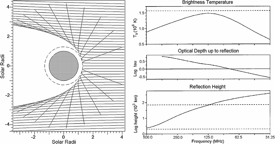
Figure 4. (Left) Ray paths at metric wavelengths, showing the effects of refraction and total reflection; figure prepared by the author. (Right) The height of reflection, the optical depth up to the reflection point and the brightness temperature as a function of frequency for the center of the solar disk. The ray tracing computations were performed for a Saito equatorial density model, with a coronal temperature of 1.52 10⁶ K and a constant conductive flux Transition Region with $F_c=10^5$ erg cm⁻² s⁻¹. Reprinted from Advances in Space Reseach, Vol 14, Alissandrakis, Radio observations of the quiet solar corona, 81–91 (1994), with permission from Elsevier.

Refraction effects are important when the optical depth between the observer and the point of total reflection is small. This is illustrated in the right panel of Figure 4, where the height of reflection, the optical depth up to reflection and the resulting brightness temperature are plotted as a function of frequency for the center of the solar disk. For frequencies higher than ~125 MHz the reflection point is inside the TR (between the dashed lines at the bottom of the figure). Moreover, radiation from the reflection point does not reach the observer because is absorbed by the overlaying layers which are optically thick; thus the brightness temperature increases with decreasing frequency, as the effective level of formation moves up through the TR toward the corona. At longer wavelengths the rays are reflected before they accumulate sufficient optical depth and the brightness temperature decreases, remaining below the coronal electron temperature (dashed line, top panel of the figure).

The above predictions are verified by observations at long (metric) wavelengths, where there is a marked departure of the brightness temperature below the coronal electron temperature, with the brightness temperature showing a maximum of ≤ 10⁶ K near 2–3 m (see Table 1 and Figure 4 of Lantos, 1999).

In addition to refraction, scattering by random density fluctuations also plays a role (Aubier et al., 1971; Hoang and Steinberg, 1977; Thejappa and Kundu, 1992, 1994; Bastian, 1994; Thejappa and MacDowall, 2008). Scattering smooths sources of small angular size; for example, Mercier et al. (2015) reported sizes no smaller than ~ 30′′ for type I bursts, although the nominal resolution of their combined NRH-GMRT observations was 20′′. Moreover, anisotropic scattering also displaces sources (Kontar et al., 2019). Finally, scattering can decrease the observed brightness at low frequencies (Thejappa and MacDowall, 2008).

4.4. Interplanetary Scintillation

Interplanetary scintillation (IPS) refers to fluctuations in the emission from distant compact radio sources on timescales of ~1 s, due to density variations in the solar wind plasma (e.g., Hewish et al., 1964; Jokipii, 1973; Bisi et al., 2010 and references therein). The analysis of IPS observations can provide estimates of the solar wind speed over global spatial scales which complement the in situ measurements from spacecraft. On the other hand, IPS is sensitive to turbulent-scale density variations which complements the larger scales accessible by white-light coronagraphs.

Classically, IPS probe the solar wind and the outer corona. However, using the Jansky VLA, information on the inner corona down to 2 R_⊙ can be obtained (Kobelski et al., 2019).

5. Horizontal structure

5.1. Theoretical Issues

The importance of horizontal structure was pointed out in section 4. A basic question that we will address here is what determines the horizontal structure. In order to answer this question we will resort to plasma physics, magnetohydrodynamics in particular (see also Chapter 2 in Priest, 1987 and Chapter 6 in Aschwanden, 2004). We will start with the MHD equation of momentum transport:

$\begin{array}{ll}\rho \left(\frac{\partial V}{\partial t}+V·\nabla V\right)=\rho g-\nabla P+\frac{J\times B}{c}& (31)\end{array}$

where V is the plasma flow velocity, B the magnetic field, J the electric current density, P the pressure and g the gravity. The magnetic field acts upon the plasma through the Lorentz force, J × B/c, which is perpendicular to the field. Using Ampère's law,

$\begin{array}{ll}\nabla \times B=\frac{4\pi }{c}J& (32)\end{array}$

we can eliminate the current in the Lorentz force to get:

$\begin{array}{ll}\frac{J\times B}{c}=-\nabla \frac{B^2}{8\pi }+\frac{B·\nabla B}{4\pi }& (33)\end{array}$

which decomposes the Lorentz force to a magnetic pressure term:

$\begin{array}{ll}{P}_m=\frac{B^2}{8\pi }& (34)\end{array}$

and a magnetic tension term which depends on the curvature of the magnetic field lines; indeed, the second term in the right hand side of (33) can be written as:

$\begin{array}{ll}\frac{B·\nabla B}{4\pi }=\frac{B^2}{4\pi }\frac{\widehat{n}}{R_c}+{\nabla }_{\Vert }\frac{B^2}{8\pi }& (35)\end{array}$

where ∇_‖ is the component of the gradient parallel to the field, $\widehat{n}$ is the unit vector perpendicular to the field and R_c is the curvature of magnetic field lines:

$\begin{array}{ll}\frac{\widehat{n}}{R_c}=\widehat{b}·\nabla \widehat{b}& (36)\end{array}$

where $\widehat{b}$ is the unit vector along the field. Going back to (33), the Lorentz force can be written as:

$\begin{array}{ll}\frac{J\times B}{c}={\nabla }_{\perp }{P}_m+\frac{B^2}{4\pi }\frac{\widehat{n}}{R_c}& (37)\end{array}$

where ∇_⊥ is the component of the gradient perpendicular to the field; the first term in the rhs is the magnetic pressure and the second is the magnetic tension.

Since the Lorentz force acts perpendicular to the field, parallel to the field we can write from (31):

$\begin{array}{ll}\rho \left(\frac{\partial V_{\Vert }}{\partial t}+V_{\Vert }·\nabla V_{\Vert }\right)=\rho g_{\Vert }-{\nabla }_{\Vert }P& (38)\end{array}$

which is Bernouli's equation of flow in a flux tube. Moreover, if the plasma motion is slow, i.e.,

$\begin{array}{ll}V\ll \sqrt{\frac{P}{\rho }}=v_s\left(\text{sound speed}\right)& (39)\end{array}$

$\begin{array}{ll}V\ll \frac{B}{\sqrt{4\pi \rho }}=v_A\left(\text{Alfvén speed}\right)& (40)\end{array}$

$\begin{array}{ll}V\ll \sqrt{Lg}~v_g\left(\text{free fall speed}\right)& (41)\end{array}$

the velocity terms in the momentum transfer equation can be ignored, and we get the hydrostatic equilibrium equation:

$\begin{array}{ll}{\nabla }_{\Vert }P=\rho g_{\Vert }& (42)\end{array}$

which is the same as (1) and has the solution:

$\begin{array}{ll}P=P_0{e}^{-{\int }_{z_0}^z\frac{dz}{H(T)}}& (43)\end{array}$

where H(T) = (kT)/(gμ_molm_H) is the scale height (cf section 3.1).

The conclusion from the above analysis is that, under the conditions specified by (39)–(41), each magnetic flux tube has its own atmosphere, as far as the pressure distribution is concerned. Moreover, since the heat conduction coefficient is much higher along the magnetic field than in the perpendicular direction, each flux tube has its own temperature distribution.

Let us now consider the equation for the time variation of the magnetic field. Starting from Ohm's law:

$\begin{array}{ll}E+\frac{V\times B}{c}=\eta J& (44)\end{array}$

where E is the electric field, J is the electric current density and η is the resistivity; substituting in Faraday's law,

$\begin{array}{ll}\nabla \times E=-\frac{1}{c}\frac{\partial B}{\partial t}& (45)\end{array}$

we obtain the induction equation:

$\begin{array}{ll}\frac{\partial B}{\partial t}=\frac{\eta c^2}{4\pi }{\nabla }^{2}B+\nabla \times (V\times B)& (46)\end{array}$

In the case of

$\begin{array}{ll}{R}_m\equiv \frac{4\pi VL}{\eta c^2}\ll 1,& (47)\end{array}$

where R_m is the magnetic Reynolds number and L is the spatial scale of the magnetic field, the second term in the right hand side of (46) can be ignored; in this case the time evolution of the field is described by a diffusion equation:

$\begin{array}{ll}\frac{\partial B}{\partial t}=\frac{\eta c^2}{4\pi }{\nabla }^{2}B& (48)\end{array}$

and magnetic energy eventually goes to thermal energy, through Joule heating. In the opposite case the second term in the right hand side of (46) dominates and the field is frozen-in:

$\begin{array}{ll}\frac{\partial B}{\partial t}=\nabla \times (V\times B)& (49)\end{array}$

Almost everywhere in the solar atmosphere the magnetic Reynolds number is much larger than unity. Thus, in quiescent situations, the behavior of the plasma and the magnetic field depends upon their relative energy density (see also Gary, 2001):

• If the energy density (thermal plus kinetic) of the plasma is much smaller than that of the magnetic field or, equivalently, if the sum of the gas pressure and the dynamic pressure is much smaller than the magnetic pressure, then the magnetic field dominates and the plasma flows along the field lines. This is the case in the chromosphere, the corona and in sunspots.

• In the opposite case the plasma dominates and will drag and deform the field. This happens in the photosphere (outside sunspots) and in the solar wind.

The situation is quite different when large amounts of energy are impulsively released, in which case both the plasma and the magnetic field are restructured.

As we will see further on in this review, this simple argument can explain qualitatively almost everything that we see on the Sun. Of course there are phenomena that require a more sophisticated approach, such as kinetic plasma theory. Today we have at our disposal both powerful computers and efficient codes for solving numerically the MHD equations and we have seen spectacular results of simulations that can hardly be distinguished from real observations (see reviews by Solanki et al., 2006; Carlsson, 2007; Nordlund et al., 2009; Moradi et al., 2010, de Wijn et al., 2009; Rempel and Schlichenmaier, 2011; see also the recent review by Carlsson et al., 2019). Still, it is very important to have a sound understanding of the physical principles which are often hidden behind the simulations.

5.2. Photospheric Structure and the Network

From the above discussion we expect plasma motion to dominate in the QS photosphere and drag the magnetic field lines (for an overview of solar magnetic fields see Wiegelmann et al., 2014 and Bellot Rubio and Orozco Suárez, 2019). Indeed, the most prominent photospheric structure is the granulation, with a spatial scale of ~1.5′′, and a temporal scale of ~15 min, which is attributed to convection currents (see the classic work by Bray and Loughhead, 1967 for a historic account and the reviews by Nordlund et al., 2009 and Rincon and Rieutord, 2018). As can be seen in Figure 5, the intensity and velocity images of the photosphere at the center of the solar disk are practically identical, which proves that hot material in the bright granules ascends, while cooler material in the dark inter-granular lanes descends; the same effect produces the zigzag appearance of photospheric absorption lines (see, e.g., Figure 6.20 in Zirin, 1988). As a matter of fact, the convection zone ends below the photosphere, which is convectively stable; thus, the granulation is an effect of overshoot of convection into the stable layers of the photosphere.

FIGURE 5

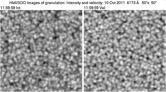
Figure 5. Image of the photospheric granulation at the center of the disk (left), together with an image of the line of sight velocity (white toward the observer). The velocity image has been averaged over 5 min to reduce the effect of oscillations. In this and subsequent figures the field of view is marked in the figure title. Images produced by the author, using data from the Helioseismic and Magnetic Imager (HMI) aboard the Solar Dynamics Observatory (SDO).

The photospheric granulation is not the only convection system on the Sun. A larger scale (~40′′) and long lived (~20 h) convection system was detected by Leighton et al. (1962), as a horizontal flow pattern; it is better visible far from the center of the disk, where the horizontal flow translates to approaching and receding line of sight velocities. This has been called supergranulation. An intermediate scale convection system, the mesogranulation has been reported by November et al. (1981), who used correlation tracking to measure horizontal flows. In the older approach, the three scales of convection would be associated with the ionization zones of HI, HeI, and HeII. However, the existence of mesogranulation as distinct scale of convection has been contested; views have been expressed that it is an extension of granulation or even an artifact produced by the correlation tracking algorithm (see discussion in Nordlund et al., 2009; Rincon and Rieutord, 2018).

The development of time-distance helioseismology has given us some information on the depth of supergranulation, despite the inherent difficulties (Nordlund et al., 2009; Kosovichev, 2011). According to Kosovichev and Duvall (1997), supergranular flows appear down to 2–3 Mm below the surface; however the pattern disappears or is dominated by noise below ~ 5 Mm. Similar results were obtained by Jackiewicz et al. (2008), see Figure 10 of Gizon et al. (2010).

Under the influence of the plasma flows the magnetic field is deformed and dragged at the edge of supergranular boundaries. The compressed magnetic flux tubes appear as tiny bright features in intergranular lanes, best visible in very high resolution photographs taken in the G-band. These were first detected by Dunn and Zirker (1973) and called filigree (see, e.g., Hα image in Figure 10, left). Higher up, in the chromosphere, enhanced emission is observed above these regions. The emission is more diffuse there, apparently due to the lateral expansion of the magnetic flux tubes. These regions of enhanced chromospheric emission constitute the well-known chromospheric network which, as pointed out by Leighton et al. (1962), coincides with the borders of the supergranules; for the region inside the supergranules the terms cell interior, or internetwork, or intranetwork are used. In spite of its name, the network has its roots in the photosphere, or even lower.

The convective flows not only drag the magnetic field; they also compress it to kilo Gauss strengths, as deduced first by Stenflo (1973), from simultaneous measurements in lines with different Landé factors. Magnetic field of such strength cannot be confined by the plasma pressure alone, thus Parker (1978) proposed that the field is further confined as a result of the adiabatic cooling of the descending plasma. Figure 6 (left) shows a magnetogram of a quiet region near the center of the solar disk; the strong network field is accompanied with brightenings in the continuum around 1700 Å (center); the strongest magnetic features are associated with persistent downflows (right). The maximum downflow is ~700 m/s, about a factor of 2 stronger than measured by Dara et al. (1987). In spite of the 4 h integration, the velocity image shows signs of granular convective motions, reminiscent of the “persistent" granulation (Baudin et al., 1997).

FIGURE 6

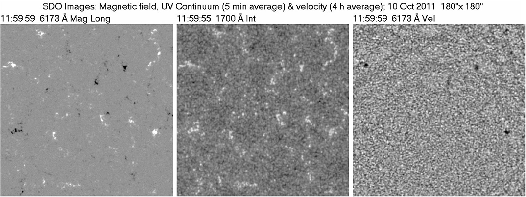
Figure 6. Line of sight magnetic field from HMI/SDO (Left), intensity in the 1700 Å band from AIA/SDO (Middle) and line of sight velocity averaged over 4 h from HMI/SDO (Right); downflows are dark, upflows bright. Images produced by the author.

The fact that the vertical component of the magnetic field is strong at superganular boundaries does not mean either that the internetwork region is devoid of field or that the field orientation is vertical everywhere. As demonstrated by the magnetogram of Figure 6, small magnetic elements are practically everywhere (Title and Schrijver, 1998).

The network is easily visible in the microwave radio range. The first high resolution images, obtained by Kundu et al. (1979) at 6 cm with the Westerbork Synthesis Radio Telescope (WSRT) showed a clear association of the microwave emission with the chromospheric network. This conclusion was subsequently verified with VLA observations at 6 and 20 cm by Gary and Zirin (1988), and Gary et al. (1990) at 3.6 cm. In the mid 90's the VLA was used for QS observations in the short cm-range (1.2, 2.0 and 3.6 cm) by a number of authors (Bastian et al., 1996; Benz et al., 1997; Krucker et al., 1997). In a more recent work, Bogod et al. (2015) reported an almost one-to-one correspondence between the microwave structures observed with RATAN-600 and those seen in the 304 Å AIA band, with a somewhat inferior correlation with the 1600 Å band.

In the mm-range, high-resolution images of the QS were first produced by White et al. (2006) and Loukitcheva et al. (2006), with the 10-element Berkeley-Illinois-Maryland Association Array (BIMA), providing ~ 10′′ resolution. With the advent of ALMA, a new collection of high-resolution mm-λ images is accumulating, with some of them presented in Figure 7. In all cases the chromospheric network, delineated in UV continuum images or photospheric magnetograms, is the dominant structure in the quiet sun radio images. The coarse network is also visible in low-resolution full-disk ALMA images, as in Figure 1 of Alissandrakis et al. (2017); at 239 GHz, these authors found best correlation with 1600 Å AIA images.

FIGURE 7

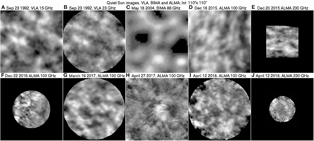
Figure 7. A collection of high-resolution radio images of the quiet Sun from the short cm-λ to the mm-λ range. (A,B) are from Bastian et al. (1996), © AAS, reproduced with permission, (C) from Loukitcheva et al. (2009), reproduced with permission © ESO, (D,E) are from ALMA commissioning, near the East and South limb respectively, (F) from Wedemeyer et al. (2020), reproduced with permission © ESO, (G) from Nindos et al. (2018), reproduced with permission © ESO, (H) from ALMA project 2016.1.00202.S used by Loukitcheva et al. (2019), while (I,J) are unpublished, courtesy of A. Nindos. The images have been reprocessed by the author for homogeneity and better visibility.

In addition to the morphology of the radio features, it is important to measure their intensity and size as a function of wavelength. We should note that normal interferometric/synthesis observations cannot measure the background level, which should be provided by other means. Thus, the most appropriate measure of the intensity fluctuations is their amplitude or their rms variation. Such measurements in the cm and mm-λ ranges have been provided by Kundu et al. (1979), Gary and Zirin (1988), Bastian et al. (1996), Benz et al. (1997), Loukitcheva et al. (2009), Nindos et al. (2018), Loukitcheva et al. (2019), and Wedemeyer et al. (2020). In all reported measurements, both the network/cell amplitude and the rms of spatial intensity variations increase with wavelength. Such results can be exploited in multicomponent models (Alissandrakis et al., 2020). Older computations by Chiuderi Drago et al. (1983), based on the Vernazza et al. (1981) model, predicted an increase of brightness difference between network and cell interiors with wavelength, in qualitative agreement with the above results.

5.3. Structure From the Upper Chromosphere to the Low Corona

Above the photosphere, the energy density of the plasma drops fast due to the decrease of the density, whereas the magnetic energy density decreases at a slower rate. Eventually the magnetic field dominates over the plasma in the QS chromosphere and low corona and, as a result, a dramatic change in the morphology of fine structures is observed. Structures of convective origin, such as granules and magnetic bright points give way to elongated structures delineating the lines of force of the magnetic field.

This is illustrated in Figure 8 where, in addition to the magnetogram of Figure 6, images of the same region in the HeII 304 Å and in the FeXII 193 Å lines, formed in the upper chromosphere/low transition region and in the corona respectively, are shown. In addition to the extension of the network, the HeII image shows a multitude of small scale, low-lying loops, mostly in absorption (dark), joining regions of opposite magnetic polarity. Although the appearance of the coronal image is different, loops are still the basic structural element; here they all are in emission (bright), they are not as numerous as in HeII and there is a lot of diffuse emission in between. The latter is probably due to low intensity loops, too thin to be distinguished with the ~ 1′′, resolving power of the instrument.

FIGURE 8

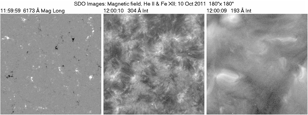
Figure 8. Line of sight magnetic field from HMI/SDO (left), intensity in the HeII 304 Å band (middle) and in the FeXII 193 Å band (right) from AIA/SDO. Same region as in Figure 6. Images produced by the author.

Note the absence of any trace of the network in the coronal image. This is well-known from the Skylab era (Reeves et al., 1974): the network becomes diffuse in the upper transition region and disappears in the low corona, apparently as a result of fanning out of the magnetic field and field lines closing at low heights. A similar behavior is expected for the radio network, the main problem here being the variable spatial resolution. However, Bastian et al. (1996) reported no detectable change in the size of network elements between 1.3 and 2 cm, after smoothing the 1.3 cm image to match the 2 cm resolution. There is a lack of imaging observations between 6 and 20 cm; in any case, the few published QS images at 20 cm do not show much of a network (e.g., Gary and Zirin, 1988).

A more classical picture of the chromospheric fine structure on the disk is shown in the top of Figure 9, in the wing and at the center of the Hα line, far from the center of the solar disk. Thin, elongated dark structures, known as dark mottles, emerge above the supergranular boundaries. They extend more or less vertically and are best visible in the blue wing of the line, revealing a predominantly upward motion. They are less prominent at the Hα line center where, in addition, fine bright mottles appear at their roots.

FIGURE 9

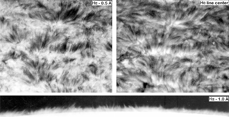
Figure 9. (Top) A chromospheric region far from the center of the solar disk, in the blue wing of Hα (left) and in the center of the line (right). The field of view is 95′′ by 80′′. Photographs by the author with the 40 cm Tourelle refractor at the Pic du Midi Observatory on September 27, 1979. (Bottom) Spicules at the limb, in the blue wing the Hα line. Observed by R. D. Dunn with the Vacuum Tower Telescope (now the Dunn Telescope) of the Sacramento Peak Observatory in 1970. Image adapted by the author from a figure published in Lynch et al. (1973).

Seen at the limb, these structures appear as jet-like features (spicules, see Secchi, 1875, Beckers, 1968, 1972; Sterling, 2000; Pasachoff et al., 2009, Tsiropoula et al., 2012), well visible in the Hα line and many other chromospheric lines and continua. Spicules have a typical lifetime of ~10 min; they rise to heights of up to ~ 10 000 km with a velocity of ~ 20 km s⁻¹ and then either fall down or diffuse in the corona. A classic spicule image, −1 Å off the Hα line center, is shown in the bottom of Figure 9. This was the best image at the time it was taken (1970); today we can have much higher spatial resolution, as evidenced in Figure 10, which shows structures as thin as a few tenths of an arc second both on the disk (left) and beyond the limb (right). High resolution imaging from space, together with the improved resolution of ground-based observations, has led to a number of recent investigations both at the limb and on the disk. The new observations revealed the existence of a new type of spicules, type II spicules (de Pontieu et al., 2007), which are both faster (~ 100 km s⁻¹) and short lived (~1 min), compared with ordinary spicules. The other domain where new observations have had an enormous contribution is spicule oscillations (see Zaqarashvili and Erdélyi, 2009 for details).

FIGURE 10

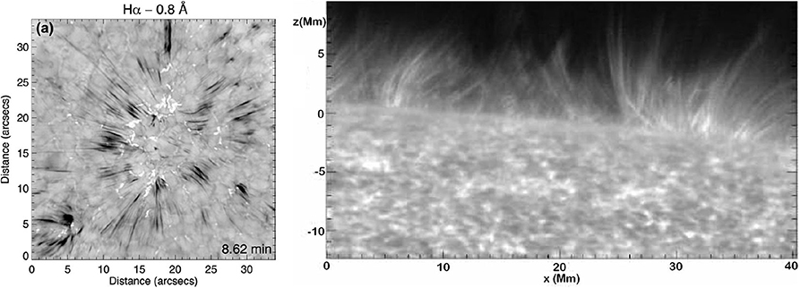
Figure 10. High resolution images of Hα spicules near the center of the disk from the Goode Solar Telescope, Big Bear (left, from Sterling et al., 2020, © AAS, reproduced with permission, based on work by Samanta et al., 2019) and at the limb observed in the CaII H line with the Solar Optical Telescope (SOT) aboard Hinode (right, from Judge and Carlsson, 2010, © AAS, reproduced with permission).

Note that the appearance of chromospheric structure in different spectral lines can be quite different, depending on the details of line formation. For example, spicules on the disk are hard to see in any other line except for Hα (see, however, Bose et al., 2019); in other lines and in the EUV continuum one can clearly see the bright emission associated to the network (Figure 10, right), as well as grains, which represent oscillating elements. Beyond the limb, structures seen in the HeII 304 Å line are much more extended than Hα spicules and are usually referred to as macrospicules.

The origin of spicules is still a subject of debate. As disk mottles are clearly associated with the network, a magnetic association is very likely; what is not clear is whether they are a result of reconnection, as suggested a long time ago by Pikel'Ner (1969), see also Samanta et al. (2019), or some other mechanism, such as the leakage of photospheric oscillations expelling plasma along the magnetic field lines, as suggested by De Pontieu et al. (2004). In a recent work, (Martínez-Sykora et al., 2017; see also Carlsson et al., 2019) obtained spicule-like features in a 2.5D radiative MHD simulation. According to these authors, spicules occur when magnetic tension is amplified and transported upward through interactions between ions and neutrals or ambipolar diffusion.

In the pre-ALMA era there has been only one report of structures beyond the limb (Habbal and Gonzalez, 1991) in the microwave range. Still, chromospheric structures have been invoked in the interpretation of the center to limb variation of the intensity, with observations showing less brightening than predicted by homogeneous models. This effect has been interpreted in terms of absorbing features, such as spicules (e.g., Lantos and Kundu, 1972; Selhorst et al., 2005). ALMA observations near the limb (Nindos et al., 2018; Yokoyama et al., 2018; Shimojo et al., 2020) do show spicular structures (Figure 11). Although the resolution is still worse than an arc second, such observations are promising for spicule diagnostics. More generally, high resolution images with ALMA can provide excellent diagnostics of the chromosphere, as the observed brightness temperature is directly related to the electron temperature and density.

FIGURE 11

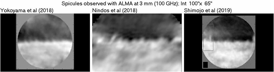
Figure 11. The first ALMA observations of spicules at 100 GHz (3 mm). Images reprocessed by the author for better visibility. The central image is reproduced with permission © ESO, the others are © AAS, reproduced with permission.

Another note-worthy observation is that polar regions are brighter than the low-latitude QS at short cm-waves to mm-waves, an effect known as polar brightening. We will not discuss this in detail here, but refer the reader to the review by Shibasaki et al. (2011).

5.4. Large Scale Structure of the Corona

The magnetic lines of force of small scale magnetic dipoles, associated with the network magnetic fields, close at relatively low heights (comparable to the distance between the opposite polarities). Thus, the coronal structure is dominated by two types of magnetic configuration: one is the medium and large scale bipolar fields associated with active regions, where the plasma is confined by the magnetic field in medium and large scale loops. The other is the so called open magnetic configuration, associated with extended regions of the same polarity; these regions cannot confine the plasma, which expands in the interplanetary medium as the fast solar wind and what is left in the corona is just a hole. An example with both closed an open regions in the corona together with the corresponding magnetogram and extrapolated magnetic field lines is presented in Figure 12.

FIGURE 12

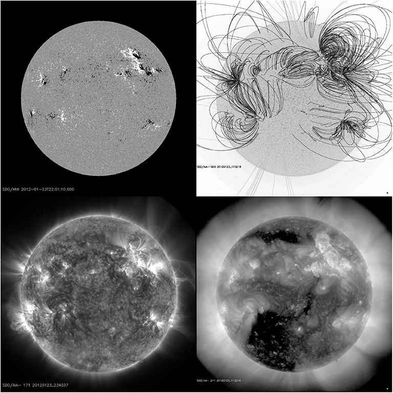
Figure 12. A full disk HMI/SDO magnetogram (top left) with extrapolated magnetic field lines (top right), the upper TR observed in the 171 Å (FeVIII) band (bottom left) and the corona observed in the 211 Å (FeXIV) band (bottom right) with AIA/SDO on January 23, 2012. Images adapted from http://suntoday.lmsal.com/suntoday/.

As we go to heights where the solar wind attains significant speed, the kinetic energy density of the plasma increases and surpasses the energy density of the magnetic field. Thus, if a closed magnetic configuration extends high enough, the tops of the outer lines of force will be dragged by the solar wind to produce the magnetic configuration of a streamer (Figure 13, left). Note that an electric current sheet (dashed line in the figure) is formed, separating regions of opposite magnetic polarity (Koutchmy and Livshits, 1992). Streamers are not cylindrically symmetric, as was thought in the past (hence the term helmet streamer), but go around the Sun, forming a belt which is often irregular, depending on the complexity of the large scale solar magnetic field; the associated current sheets extends into the interplanetary space, forming the heliosheet that separates opposite magnetic polarities in the heliosphere. Streamers may also form in more complex (quadrupole) magnetic field configurations (Koutchmy et al., 1994).

FIGURE 13

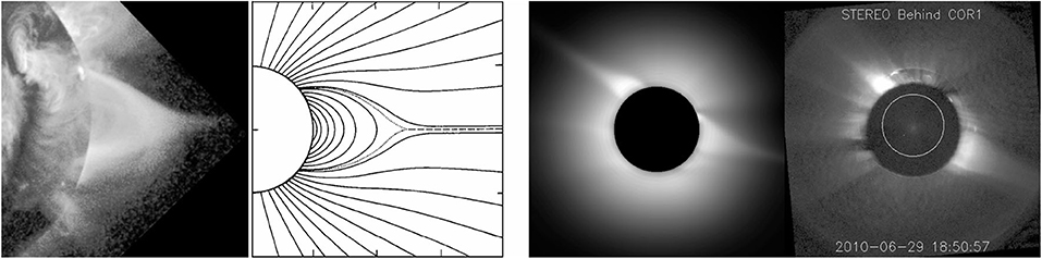
Figure 13. From left to right: A streamer observed with Yohkoh; a schematic drawing of the corresponding magnetic configuration; computed intensity of the corona based on the MAS code; the corresponding image of the COR1 coronograph aboard STEREO-B, on June 29, 2010. From http://www.predsci.com/stereo/home.php.

The magnetic field lines of force shown in Figure 12 have been computed under the current-free assumption, using the photospheric magnetic field as a lower boundary condition (Schmidt, 1964 in plane geometry; Altschuler and Newkirk, 1969 in spherical geometry and for the entire Sun; see Chapter 5 in Aschwanden, 2004 for a more detailed discussion). In the more general case of the force free approximation, the electric current is assumed to flow along the magnetic field, so that Ampère's law, (32), takes the form:

$\begin{array}{ll}\nabla \times B=\alpha B& (50)\end{array}$

which includes the current-free case (α = 0). In this case the Lorentz force vanishes, hence the term force-free. It is easy to prove that α is constant along a magnetic field line, by taking the divergence of (50). If α is assumed constant everywhere, we have the linear force free case; this is relatively easy to compute (Alissandrakis, 1981), compared to the non-linear case (Wiegelmann and Sakurai, 2012; Wiegelmann et al., 2017).

One can go further by taking into account the full set of MHD equations, and compute, in addition to the magnetic field, the density of the plasma, as well as the flow velocity in 3 dimensions. An example is shown at the right of Figure 13, where the coronal intensity has been computed with the Magnetohydrodynamic Algorithm outside a Sphere (MAS) code (Riley et al., 2011; see also Wiegelmann et al., 2017). Despite the fact that the computation is based on magnetic field data over a full solar rotation (26 days), the similarity with the observed corona is remarkable, in particular for large scale structures (such as streamers), which are also long-lived.

The corona is accessible with radio observations in the metric region, but here one has to be content with arc-minute resolution. The first images were obtained with the Culgoora Radioheliograph at 80 MHz (3.75 m) and 160 MHz (1.88 m), followed by the Clark Lake Radioheliograph at 73.8 MHz (4.07 m), 50 MHz (6 m), and 30.9 MHz (9.7 m). The first 2D images from the Nançay Radioheliograph (NRH) were computed by Alissandrakis et al. (1985) at 169 MHz (1.78 m) with 1.2′ by 4.2′ resolution.

The NRH evolved gradually to its present state of 2D synthesis instrument (Kerdraon and Delouis, 1997), providing images at 10 frequencies from 450 to 150 MHz (67 cm to 2 m) with a cadence of 0.25 s. The instantaneous images, however, cannot exploit the full resolution of the system since they only use the densely sampled inner part of the u-v plane. In order to exploit the full resolution one has to resort to full-day synthesis, which improves the resolution by a factor of ~ 2.5. This was done by Marqué (2004) with an emphasis on filament cavities and subsequently by Mercier and Chambe (2009, 2012, 2015), who did a systematic study of the quiet Sun. The NRH covers a broad range of frequencies, the ratio of the maximum to minimum frequency being ~ 3; it can thus probe an altitude range from the upper TR to the low corona. Shibasaki et al., 2011 give some examples of synthesis images from NRH in their Figure 7.

Mercier and Chambe (2015) found that the temperature deduced from the hydrostatic scale height (1.5 × 10⁶ K) was too high compared to the brightness temperature of the solar disk (0.60 to 0.65 × 10⁶ K at 150 MHz) and suggested that the electron temperature in the corona (contributing to observed brightness) is lower than the proton temperature (mainly responsible for the hydrostatic scale). More recently, QS images in the decametric range, obtained with the Low Frequency Array (LOFAR), were presented by Vocks et al. (2018), in the range of 25 to 79 MHz. They give brightness temperatures of the order of 10⁶ K at 54 MHz, which are higher than the values of Mercier and Chambe (2015) and previous measurements given in section 4.3.2; they also deduced high hydrostatic temperatures, up to 2.2 × 10⁶ K. These results show that more work is necessary in order to settle the issue of interpretation of the QS metric-decametric emission. In addition to NRH and LOFAR, the Murchison Widefield Array (MWA) have started providing interesting QS data (McCauley et al., 2019; Rahman et al., 2019) with high dynamic range.

Coronal holes are usually observed as brightness depressions in radio wavelengths (e.g., Borovik and Medar, 1999; Lantos and Alissandrakis, 1999). At cm-λ the average brightness temperature in coronal hole regions is not much different from that of the quiet Sun, while at mm-λ it is slightly higher (Gopalswamy et al., 2000), apparently due to the underlying chromosphere and TR, rather than the coronal holes. A number of computations of the coronal hole radio emission (e.g., Borovik et al., 1990; Chiuderi Drago et al., 1999; Pohjolainen, 2000) have been published. Borovik et al. (1990) observed four coronal holes in the wavelength range of 2 to 32 cm with the RATAN-600 telescope and found that the brightness difference between the holes and the QS becomes appreciable at wavelengths longer than ~ 4 cm. In their best-fit models the coronal holes are cooler than the background and less dense by a factor of 2.

The work of Mercier and Chambe (2009) confirmed that, at long dm wavelengths, coronal holes are the most prominent feature; in agreement with previous observations (e.g., Lantos et al., 1987), their contrast decreases at longer wavelengths (see the hole near the center of the disk in Figure 3 of Mercier and Chambe, 2009). At decameter waves coronal holes are sometimes seen in emission (Dulk and Sheridan, 1974; Lantos et al., 1987; Rahman et al., 2019). A possible interpretation is in terms of refraction effects (Alissandrakis, 1994, c.f. Figure 3 of Lantos, 1999) and/or scattering in inhomogeneities; a similar conclusion was reached by Rahman et al. (2019). In addition, these authors computed metric solar images using parameters derived from the MAS code (see above) and found qualitative similarities with high frequency observations, but could not reproduce the dark-to-bright transition at low frequencies. McCauley et al. (2019) measured the polarization of coronal holes and reported values up to 5–8%; they also reported a “bullseye" polarization structure, in which one polarization sense is surrounded by a full or partial ring of the opposite sense (see their Figure 7).

In a systematic study of emission sources observed with the NRH at 169 MHz, Lantos and Alissandrakis (1999) came to the conclusion that the large scale emission is dominated by the coronal plateau. This is an intermediate brightness region forming a belt around the Sun and surrounding almost all local emission sources (Lantos et al., 1992). It is visible both in daily images and in synoptic charts, and has a close association with enhanced emission of the K-corona, delineating the base of the coronal plasma sheet. The diffuse emission of the coronal plateau could be due to a high altitude loop system which overrides the principal neutral line of the general solar magnetic field at the base of the heliosheet, with a possible contribution of loops connecting active regions to surrounding quiet areas.

Coronal streamers are best visible at decametric wavelengths (Lantos, 1999). They are less prominent in the meter and decimeter ranges, where one sees loops at the base of streamers rather than proper streamers, as pointed out in the previous paragraph. From the circularly polarized thermal emission of streamers observed with the Gauribidanur radioheliograph at 77 and 109 MHz, Ramesh et al. (2010) estimated magnetic field strengths in the range of 5 – 6 G at 1.5 – 1.7 R_⊙.

5.5. Filaments and Prominences

The configuration of the magnetic field above neutral lines of the magnetic field is such that, under certain topologies, it can sustain clouds of material of chromospheric temperature and density against gravity and thermally isolate them from the hot corona. In chromospheric lines and on the solar disk, these clouds appear in absorption as filaments; projected beyond the solar disk, they appear in emission as prominences (see reviews by Labrosse et al., 2010 and Mackay et al., 2010).

At decimeter-meter wavelengths (Marqué, 2004), as well as in the mm and cm range (Irimajiri et al., 1995) large filaments are observed as regions of lower brightness temperature on the solar disk. Beyond the limb filaments are seen in emission, projected against the sky; in this case it is possible to calculate electron temperatures and densities using multi-frequency radio observations (Irimajiri et al., 1995). Filaments, filament cavities and prominences show well in full-disk ALMA images at 1.25 and 3 mm (see, e.g., Figure 1 in Alissandrakis et al., 2017).

A set of simultaneous observations of a filament in the microwave range and in the EUV was analyzed by Chiuderi Drago et al. (2001). The authors concluded that the depression at radio wavelengths is due to the lack of coronal emission; the same data favored a prominence model with cool threads embedded in the hot coronal plasma, enveloped by a sheath-like TR, and a filling factor varying from about 3 to 4%.

A systematic study of filaments and their environment in the metric radio range was presented by Marqué (2004). He used NRH observations primarily at 410.5 MHz, pointing out that the visibility of filament associated radio depressions is rather poor at lower frequencies. He concluded that the most likely source of the radio depression is the cavity (electron density depletion) that surrounds the filament. In cm and mm wavelengths contradictory results have been reported on the contribution of the cavity to the observed radio depression (Kundu and McCullough, 1972; Raoult et al., 1979).

6. Active Regions

Active Regions appear in the photosphere as roughly bipolar magnetic regions of intermediate scale (~ 0.2R_⊙, or ~ 1.5 × 10⁵ km). Sunspots, associated with strong magnetic fields (above ~1000 G), are their primary manifestation in the photosphere, bright plage emission, associated with intermediate magnetic fields, prevails in the chromospheric layers together with elongated fibrils (Foukal, 1971; Kianfar et al., 2020), indicating a more organized magnetic field compared to the QS, while impressive loops mark their presence in the corona. They are accompanied by all sorts of dynamic phenomena, most notably flares and Coronal Mass Ejections (CMEs).

Active regions are the result of emergence of large quantities of magnetic flux from the subphotospheric layers, a result of magnetic buoyancy (see, e.g., Parker, 1955; Priest, 1987; Rempel and Schlichenmaier, 2011) and disappear as their magnetic flux is spread out due to convective motions or canceled near polarity inversion lines.

Figure 14 shows images of an active region from the photosphere to the low corona, during its emergence and development phase, as the region crosses the solar disk. Concentrating on the radio emission, we note that in the 17 GHz images of July 30, as well as of August 2 and 4 show the classic two components of sunspot and plage associated emission, identified for the first time by Kundu (1959) with a 2-element interferometer and imaged by Kundu and Alissandrakis (1975) with the Westerbork Synthesis Radio Telescope. Since that time many observations and models have been published (see reviews by Gelfreikh, 1998 and Lee, 2007). It is well-established that the sunspot, or core component of the emission, observed in the microwave range, is due to the gyroresonance process (Kakinuma and Swarup, 1962; Zheleznyakov, 1962; Alissandrakis et al., 1980), whereas the plage, or halo component is due to free-free emission.

FIGURE 14

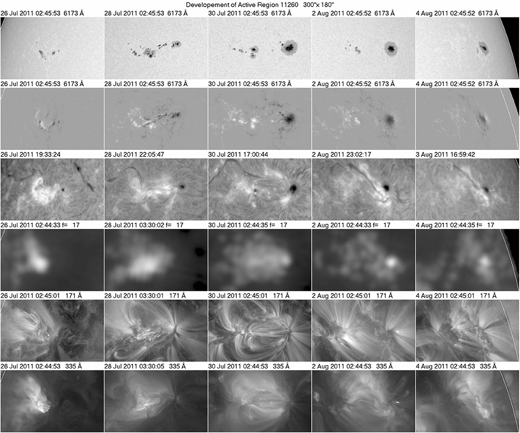
Figure 14. Development of Active Region 11260 during its passage on the solar disk. Sunspots and magnetograms from HMI/SDO, Hα images from Big Bear, Nobeyama images at 17 GHz and AIA/SDO images in the 171 Å (FeIX, log T ~ 5.8), and 335 Å (FeXVI, log T ~ 6.4) bands. The region crossed the central meridian on July 30, ~9 UT. The white arc marks the photospheric limb. Figure prepared by the author.

Going back to Figure 14, note that no sunspot component is visible at 17 GHz on the other days, apparently due to the low value of the sunspot field with regard to the observing frequency. Note also that on July 26 and 28, emission as strong as the sunspot emission is observed, probably associated with hot coronal loops seen in the 335 Å, (FeXVI) band. This is reminiscent of the neutral line sources reported by Kundu et al. (1977), see also Uralov et al. (2008) and references therein, and attributed to a quasi-steady, low density population of non-thermal electrons (Alissandrakis et al., 1993).

At longer wavelengths a decimetric halo component of non-thermal nature has been reported (Gelfreikh, 1998), while at even longer decimetric and metric wavelengths no sunspot-associated emission is visible, presumably due to the high opacity of the overlaying plasma and refraction effects; we do see, however, non-thermal noise-storm sources in the vicinity of active regions.

The microwave emission of active regions is a powerful diagnostic of the magnetic field in the transition region and the low corona. The magnetic field determines the emissivity of gyroresonance process above sunspots, of the free-free process above plages, as well as the circular polarization inversion higher up. In addition to the magnetic field, sunspot-associated emission can provide information about the temperature and density structure of the sunspot atmosphere (Nindos et al., 1996; Korzhavin et al., 2010; Nita et al., 2018; Stupishin et al., 2018; Alissandrakis et al., 2019). Let us also mention in passing the detection and study of sunspot oscillations (Gelfreikh et al., 1999; Nindos et al., 2002) and refer the reader to the review by Nindos and Aurass (2007) for more details. We also refer the reader to the reviews by Solanki (2003) and by Rempel and Schlichenmaier (2011) for extensive descriptions of sunspots.

7. Heating of the Chromosphere and the Corona

7.1. The Problem

Elementary thermodynamics tells us that you cannot transfer energy from a cold body to a hot body through radiation, conduction or convection. How do you then explain the temperature minimum and the subsequent temperature rise in the chromosphere and the corona and the energy carried away by the solar wind? The obvious answer is that you have to transport energy from below by mechanical means. As for the amount of energy required, this is of the order of 4 × 10⁶ erg cm⁻² s⁻¹ for the quiet chromosphere and about a factor of 10 lower for the quiet corona (Withbroe and Noyes, 1977).

The first answer to the heating problem was proposed more than 70 years ago, by Schwarzschild (1948) and by Schatzman (1949): the chromosphere and the corona are heated by the dissipation of shock waves, originating as acoustic waves in the noise produced by the granulation and steepened as they propagate upwards in regions of decreasing density. The discovery of the 5-min oscillations gave a boost to this idea, still other ideas, more promising, have been advanced. In what follows we will discuss some concepts and constrains with regard to the heating problem. Obviously, we cannot be exhaustive, so we refer the reader to Chapter 6 of Priest (1987), Chapter 9 of Aschwanden (2004) and reviews by Withbroe and Noyes (1977), Walsh and Ireland (2003), Klimchuk (2006), Erdélyi and Ballai (2007), Cranmer and Winebarger (2019) and Carlsson et al. (2019).

First of all, the question is not that of bulk heating, as the upper solar atmosphere is highly structured (section 5). In the chromosphere, for example, we need to supply more energy to the network, which is brighter, more dense and more dynamic than the internetwork regions. In the corona, each individual flux tube has its own energy requirement. A loop will become visible in a particular spectral line, if it contains enough plasma at the appropriate temperature; this plasma presumably comes from the chromosphere, through evaporation induced by the deposition of energy somewhere in the loop. Open flux tubes in coronal holes must also be heated, both for their own sake and in order to provide energy to the plasma that makes the fast solar wind. Note also that coronal heating requirements vary during the solar cycle, as evidenced by the great variations in X-ray brightness revealed by Yohkoh images (see, e.g., Takeda et al., 2019). Thus, the problem is not just to have an abundance of wave or some other form of mechanical energy, but mainly to transport and dissipate the energy at the proper place and at the proper time.

The magnetic field plays the primary role in determining the structure of the upper atmosphere (section 5); we also expect the magnetic field to influence the propagation of acoustic waves and, in addition, to provide plenty of additional wave modes. Wave heating, which is commonly referred to as AC heating, is not the only possibility. At the photospheric level, magnetic flux tubes (section 5.3) are known to be in continuous motion, as shown in Figure 15, in response to horizontal convective flows. As a result waves could be excited but, what is probably more important, the magnetic lines of force, which extend up in the chromosphere and the corona, will become tangled, accumulating magnetic energy in innumerable current sheets. This magnetic energy cannot accumulate in perpetuo, it will eventually be converted to heat (DC heating) in the course of reconnection, either through Joule dissipation (Equation 46), or through collisionless processes. Note that these processes could also accelerate particles that will eventually depose their energy in the plasma; these particles should have observable consequences both in the radio and the hard X-ray range.

FIGURE 15

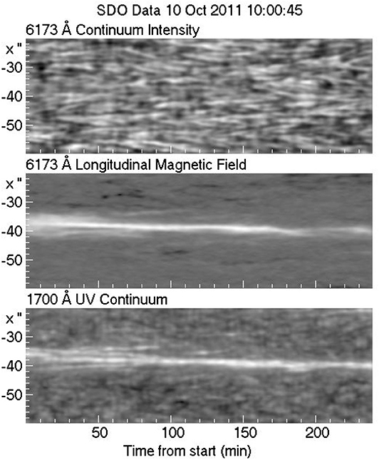
Figure 15. Position (vertical axis) - time (horizontal axis) cuts through a magnetic element. Granular motions are clearly visible in the top panel; the middle and the bottom panels show the motion of the magnetic element and the corresponding bright point in the 1700 Å band. A low pass filter has been applied in the time domain to reduce the effect of the 5 min oscillations. Figure prepared by the author from SDO data.

Reconnection mechanisms have been invoked to explain energy release in flares, hence the concept of nanoflare heating, first proposed by Parker (1988). Nanoflares are impulsive by nature and are expected to occur in elemental flux tubes that are below the resolution limit of present-day instruments. Impulsiveness is not limited to nanoflares, but may characterize AC heating as well (Klimchuk, 2006).

A radically different approach has been advanced by Scudder (1992), that the coronal plasma originates from suprathermal particles in the transition region, which have enough energy to overcome gravity (velocity filtration). However, this model requires a mechanism to produce the suprathermal particles as well as collisionless conditions, of which none is proven.

Although we have plenty of mechanisms, we have no answer yet as to which mechanism(s) may operate and in which case. As a matter of fact, we have plenty of negative answers. It is encouraging that there is sufficient energy associated with the granulation noise, as already pointed out by Schatzman (1949) and also in the random motion of magnetic flux tubes (Alissandrakis and Einaudi, 1997; Klimchuk, 2006), but this is not enough, as pointed up above, since this energy must be directed to the right place at the right time. Nanoflare heating is certainly attractive, but it evades observational confirmation so far. Several authors have computed histograms of the energy distribution in impulsive events, including microflares observed in abundance with RHESSI and other missions (Hannah et al., 2011); the extrapolation to low energies only gave negative results as far as heating is concerned. Acoustic wave heating has been a favorite for the non-magnetic chromosphere, but it appears that the appropriate waves do not carry enough energy (Fossum and Carlsson, 2005). Other types of waves, such as Alfvén waves in the presence of turbulence (van Ballegooijen et al., 2011), might help; in this context, the recently reported kink-backs in the solar wind magnetic field (Kasper et al., 2019) observed by the Parker Solar Probe, might have a bearing.

Let us finally note that, in addition to heating the upper chromosphere, one has to replenish the corona with the mass lost through the solar wind. This is not considered a problem since, as it has been shown a long time ago (Beckers, 1972), spicules that diffuse into the corona carry more mass than is actually required.

7.2. Pertinent Radio Data

We will now summarize radio observations that might have a bearing to the heating problem (see also Alissandrakis and Einaudi, 1997 and Shibasaki et al., 2011). Radio fine structures show time variability comparable to that of the chromospheric network, on time scales of minutes to hours (Erskine and Kundu, 1982; Bastian et al., 1996). Apart from that, it is important to check for oscillatory behavior, which could be a signature of shock waves heating the upper solar atmosphere. White et al. (2006) reported intensity oscillations at 3.5 mm with rms brightness variation of 50–150 K and periods of 3 to 5 min (frequencies of 3.3 to 5.5 mHz). In a recent work with ALMA, Patsourakos et al. (2020) observed oscillations at 3 mm, with frequencies of 4.2 ± 1.7 mHz and rms variation of 55 to 75 K.

A number of authors have looked for impulsive/transient events that might have a bearing on the heating of the upper atmosphere (Gary et al., 1997; Krucker et al., 1997; Benz and Krucker, 1999; Krucker and Benz, 2000). Transient brightenings are observed in microwaves both within and well-away from active regions and both thermal and non-thermal emission mechanisms have been suggested (White et al., 1995; Nindos et al., 1999); it thus seems that electrons are accelerated to non-thermal energies even in the quiet solar atmosphere. There appears to be a continuity between bursts, the radio counterparts of X-ray bright points (see Keller and Krucker, 2004 and references therein), and smaller transient events. In a recent work, Nindos et al. (2020) reported non-impulsive transients from 3 mm ALMA observations, providing ~1% of the energy of chromospheric losses. Moreover, Mondal et al. (2020) detected a large number of low intensity impulsive QS emissions with the MWA in the frequency range of 98 to 160 MHz, that might be signatures of heating events.

We may conclude that radio observations can provide important input to the problem of the heating of the chromosphere and the corona, both in the wave and nano-flare heating scenarios. Instruments with dense coverage of the u-v plane as well as improved image reconstruction techniques are necessary, in order to provide accurate instantaneous images of regions with complex structure.

8. Final comments

In addition to being our source of life, the Sun is also the nearest star (hence the stellar prototype) and an immense laboratory of plasma physics. During the last few decades we have accumulated a tremendous amount of knowledge on how the Sun operates and how it affects our daily life, thanks to the development of new instruments, both ground-based and space- borne, and the advances in the theory and numerical simulations.

An important ingredient of the recent progress is the exploitation of information from all spectral ranges. The radio domain is a basic source of information. In this respect, it is in synergy rather than in competition with the EUV and X-ray domains which also provide information about the same layers of the solar atmosphere and for the same phenomena. We should stress, however, that the interpretation of radio data, at least for the Quiet Sun and a good part of active phenomena, is straight forward; it is not plagued by non-LTE effects, uncertainties in excitation and ionization equilibrium and abundances, as are other wavelength ranges. The weakness of radio is the low spatial resolution, but this can be overcome with large synthesis instruments, without having to go to space. There are several such projects under development. Among this new generation of radio instruments, LOFAR has already provided very interesting new results, ALMA is entering dynamically into the field, the Expanded Owens Valley Solar Array (EOVSA) has started providing nice spectral imaging data, the MWA is giving interesting QS data, the Siberian Radioheliograph (SRH) is starting, the Chinese Mingantu Ultrawide Spectral Radioheliograph (MUSER) is in operation, the next generation VLA (ngVLA) is under consideration, while the Square Kilometer Array (SKA) is not too far below the horizon.

What can we expect to learn about the QS from those new instruments? Here is a partial list, reflecting the views of the author and by no means exhaustive:

• Better diagnostics of the physical conditions in all structures of the solar upper atmosphere.

• Better atmospheric models, both in the classic radial/multi-component approach and in the context of radiative MHD; among others, differences between network and cell interior conditions, as well as conditions in spicules and small-scale dynamic events, will be better measured and understood.

• Measurement of the temperature amplitude of chromospheric oscillations as a function of height.

• Improved understanding and modeling of the large-scale magnetic field in the corona.

• Filaments, filament cavities and prominences will be better diagnosed and modeled.

• Better diagnostics and understanding of the active region atmosphere.

• Better understanding of the QS emission at metric wavelengths and reconciliation with optical data.

• If nanoflares have any bearing to chromospheric/coronal heating, the energetic electrons produced should have observable signatures somewhere in the radio range.

• Last but not least, there will be new, unpredictable, discoveries as is usually the case when novel instruments become operational.

As it is always the case, as we learn more, old questions are answered, at least partially, and new questions emerge. With the new instrumentation currently under development and the continued effort on the theoretical side, we will certainly give important results in the next few years.

Author Contributions

The author confirms being the sole contributor of this work and has approved it for publication.

Conflict of Interest

The author declares that the research was conducted in the absence of any commercial or financial relationships that could be construed as a potential conflict of interest.

Acknowledgments

This review is based on a presentation to a CESRA summer school on solar radio physics. The author would like to thank Dr. L. Klein of Meudon observatory for organizing the school and for comments on an early version of the manuscript. This work makes use of the following ALMA data: ADS/JAO.ALMA#2011.0.00020.SV and ADS/JAO.ALMA2016.1.00202.S. ALMA is a partnership of ESO (representing its member states), NSF (USA) and NINS (Japan), together with NRC (Canada) and NSC and ASIAA (Taiwan), and KASI (Republic of Korea), in cooperation with the Republic of Chile. The Joint ALMA Observatory is operated by ESO, AUI/NRAO, and NAOJ. In preparing this review the author used publicly available data from a number of instruments: the Nobeyama Radioheliograph (NoRH), the Siberian Solar Radio Telescope (SSRT), the Mauna Loa Solar Observatory (MLSO), the Big Bear Solar Observatory (BBSO), the Yohkoh mission, the Solar Terrestrial Environment Observatory (STEREO), the Helioseismic and Magnetic Imager (HMI) and the Atmospheric Imaging Assembly (AIA) aboard the Solar Dynamics Observatory (SDO), the Predictive Science Inc. website (http://www.predsci.com/stereo/home.php) and the Sun Today website (http://suntoday.lmsal.com/suntoday/). I am grateful to all those that operate these instruments and make their data available to the community.

References

Ahmad, Q. R., Allen, R. C., Andersen, T. C., Anglin, J. D., Barton, J. C., Beier, E. W., et al. (2002). Direct evidence for neutrino flavor transformation from neutral-current interactions in the sudbury neutrino observatory. Phys. Rev. Lett. 89:011301. doi: 10.1103/PhysRevLett.89.011301

PubMed Abstract | CrossRef Full Text | Google Scholar

Alissandrakis, C. E. (1981). On the computation of constant alpha force-free magnetic field. Astron. Astrophys. 100, 197–200.

Google Scholar

Alissandrakis, C. E. (1994). Radio observations of the quiet solar corona. Adv. Space Res. 14, 81–91.

Google Scholar

Alissandrakis, C. E., Bogod, V. M., Kaltman, T. I., Patsourakos, S., and Peterova, N. G. (2019). Modeling of the sunspot-associated microwave emission using a new method of dem inversion. Solar Phys. 294:23. doi: 10.1007/s11207-019-1406-x

CrossRef Full Text | Google Scholar

Alissandrakis, C. E., and Einaudi, G. (1997). “Radio observations of the quiet sun and their implications on coronal heating,” in Coronal Physics from Radio and Space Observations, Lecture Notes in Physics, Vol. 483, ed G. Trottet (Springer), 53. doi: 10.1007/BFb0106451

CrossRef Full Text | Google Scholar

Alissandrakis, C. E., and Gary, D. E. (2020). Radio measurements of the magnetic field in the solar chromosphere and the corona. Front. Astron. Space Sci. doi: 10.3389/fspas.2020.591075

PubMed Abstract

Alissandrakis, C. E., Gel'Frejkh, G. B., Borovik, V. N., Korzhavin, A. N., Bogod, V. M., Nindos, A., et al. (1993). Spectral observations of active region sources with RATAN-600 and WSRT. Astron. Astrophys. 270, 509–515.

Google Scholar

Alissandrakis, C. E., Kundu, M. R., and Lantos, P. (1980). A model for sunspot associated emission at 6 CM wavelength. Astron. Astrophys. 82, 30–40.

Google Scholar

Alissandrakis, C. E., Lantos, P., and Nicolaidis, E. (1985). Coronal structures observed at metric wavelengths with the Nançay radioheliograph. Solar Phys. 97, 267–282.

Google Scholar

Alissandrakis, C. E., Nindos, A., Bastian, T. S., and Patsourakos, S. (2020). Modeling the quiet Sun cell and network emission with ALMA. Astron. Astrophys. 640:A57. doi: 10.1051/0004-6361/202038461

CrossRef Full Text | Google Scholar

Alissandrakis, C. E., Patsourakos, S., Nindos, A., and Bastian, T. S. (2017). Center-to-limb observations of the sun with alma. Implications for solar atmospheric models. Astron. Astrophys. 605:A78. doi: 10.1051/0004-6361/201730953

CrossRef Full Text | Google Scholar

Allen, C. W. (1947). Interpretation of electron densities from corona brightness. Mon. Notices R. Astron. Soc. 107:426.

Google Scholar

Altschuler, M. D., and Newkirk, G. (1969). Magnetic fields and the structure of the solar corona. I: methods of calculating coronal fields. Solar Phys. 9, 131–149.

Google Scholar

Appourchaux, T., Belkacem, K., Broomhall, A. M., Chaplin, W. J., Gough, D. O., Houdek, G., et al. (2010). The quest for the solar g modes. Astron. Astrophys. Rev. 18, 197–277. doi: 10.1007/s00159-009-0027-z

CrossRef Full Text | Google Scholar

Appourchaux, T., and Corbard, T. (2019). Searching for g modes. II. Unconfirmed g-mode detection in the power spectrum of the time series of round-trip travel time. Astron. Astrophys. 624:A106. doi: 10.1051/0004-6361/201935196

CrossRef Full Text | Google Scholar

Aschwanden, M. J. (2004). Physics of the Solar Corona. An Introduction. Chichester; Berlin: Praxis Publishing Ltd.; Springer-Verlag.

Google Scholar

Athay, R. G. (1971). “The chromosphere-corona transition region,” in Physics of the Solar Corona, Vol. 27 of Astrophysics and Space Science Library, ed C. J. Macris (Dordrecht: Reidel), 36. doi: 10.1007/978-90-277-0204-3_4

CrossRef Full Text | Google Scholar

Aubier, M., Leblanc, Y., and Boischot, A. (1971). Observations of the quiet Sun at decameter wavelengths - Effects of scattering on the brightness distribution. Astron. Astrophys. 12:435.

Google Scholar

Bastian, T. S. (1994). Angular scattering of solar radio emission by coronal turbulence. Astrophys. J. 426:774.

Google Scholar

Bastian, T. S., Dulk, G. A., and Leblanc, Y. (1996). High-resolution microwave observations of the quiet solar chromosphere. Astrophys. J. 473:539.

Google Scholar

Bastian, T. S., Ewell, M. W. J., and Zirin, H. (1993). The center-to-limb brightness variation of the sun at lambda = 850 microns. Astrophys. J. 415:364.

Google Scholar

Basu, S. (2016). Global seismology of the Sun. Liv. Rev. Solar Phys. 13:2. doi: 10.1007/s41116-016-0003-4

CrossRef Full Text | Google Scholar

Basu, S., Christensen-Dalsgaard, J., Chaplin, W. J., Elsworth, Y., Isaak, G. R., New, R., et al. (1997). Solar internal sound speed as inferred from combined BiSON and LOWL oscillation frequencies. Mon. Notices R. Astron. Soc. 292, 243–251.

Google Scholar

Baudin, F., Molowny-Horas, R., and Koutchmy, S. (1997). Granulation and magnetism in the solar atmosphere. Astron. Astrophys. 326, 842–850.

Google Scholar

Beckers, J. M. (1968). Solar Spicules (Invited Review Paper). Solar Phys. 3, 367–433.

Google Scholar

Beckers, J. M. (1972). Solar Spicules. Annu. Rev. Astron. Astrophys. 10:73.

Google Scholar

Bellot Rubio, L., and Orozco Suárez, D. (2019). Quiet Sun magnetic fields: an observational view. Liv. Rev. Solar Phys. 16:1. doi: 10.1007/s41116-018-0017-1

CrossRef Full Text | Google Scholar

Benz, A. O., and Krucker, S. (1999). Heating events in the quiet solar corona: multiwavelength correlations. Astron. Astrophys. 341, 286–295.

Google Scholar

Benz, A. O., Krucker, S., Acton, L. W., and Bastian, T. S. (1997). Fine structure of the X-ray and radio emissions of the quiet solar corona. Astron. Astrophys. 320, 993–1000.

Google Scholar

Bisi, M. M., Jackson, B. V., Breen, A. R., Dorrian, G. D., Fallows, R. A., Clover, J. M., et al. (2010). Three-dimensional (3-D) reconstructions of EISCAT IPS velocity data in the declining phase of solar cycle 23. Solar Phys. 265, 233–244. doi: 10.1007/s11207-010-9594-4

CrossRef Full Text | Google Scholar

Bogod, V. M., Alissandrakis, C. E., Kaltman, T. I., and Tokhchukova, S. K. (2015). Ratan-600 observations of small-scale structures with high spectral resolution. Solar Phys. 290, 7–20. doi: 10.1007/s11207-014-0526-6

CrossRef Full Text | Google Scholar

Borovik, V. N., Kurbanov, M. S., Livshits, M. A., and Ryabov, B. I. (1990). Coronal holes on the background of the quiet sun - Analysis of RATAN-600 observations in the 2-32-cm range. Astron. Z. 67, 1038–1052.

Google Scholar

Borovik, V. N., and Medar, V. G. (1999). “Coronal holes at microwaves as based on observations with the RATAN-600 radiotelescope,” in 8th SOHO Workshop: Plasma Dynamics and Diagnostics in the Solar Transition Region and Corona, volume 446 of ESA Special Publication, eds J. C. Vial and B. Kaldeich-Schü, 185.

Google Scholar

Bose, S., Henriques, V. M. J., Joshi, J., and Rouppe van der Voort, L. (2019). Characterization and formation of on-disk spicules in the Ca II K and Mg II k spectral lines. Astron. Astrophys. 631:L5. doi: 10.1051/0004-6361/201936617

CrossRef Full Text | Google Scholar

Bray, R. J., and Loughhead, R. E. (1967). The Solar Granulation. London: Chapman & Hall.

Google Scholar

Carlsson, M. (2007). “Modeling the solar chromosphere,” in The Physics of Chromospheric Plasmas, Vol. 368 of Astronomical Society of the Pacific Conference Series, eds P. Heinzel, I. Dorotovič, and R. J. Rutten (San Francisco, CA), 49.

Google Scholar

Carlsson, M., De Pontieu, B., and Hansteen, V. H. (2019). New view of the solar chromosphere. Annu. Rev. Astron. Astrophys. 57, 189–226. doi: 10.1146/annurev-astro-081817-052044

CrossRef Full Text | Google Scholar

Charbonneau, P. (2010). Dynamo models of the solar cycle. Liv. Rev. Solar Phys. 7:3. doi: 10.12942/lrsp-2010-3

CrossRef Full Text | Google Scholar

Chiuderi Drago, F., Alissandrakis, C. E., Bastian, T., Bocchialini, K., and Harrison, R. A. (2001). Joint EUV/Radio observations of a solar filament. Solar Phys. 199, 115–132. doi: 10.1023/A:1010390726242

CrossRef Full Text | Google Scholar

Chiuderi Drago, F., Kundu, M. R., and Schmahl, E. J. (1983). Network to cell contrast at microwaves. Solar Phys. 85, 237–242.

Google Scholar

Chiuderi Drago, F., Landi, E., Fludra, A., and Kerdraon, A. (1999). EUV and radio observations of an equatorial coronal hole. Astron. Astrophys. 348, 261–270.

Google Scholar

Christensen-Dalsgaard, J. (2002). Helioseismology. Rev. Mod. Phys. 74, 1073–1129. doi: 10.1103/RevModPhys.74.1073

CrossRef Full Text | Google Scholar

Cranmer, S. R., and Winebarger, A. R. (2019). The properties of the solar corona and its connection to the solar wind. Annu. Rev. Astron. Astrophys. 57, 157–187. doi: 10.1146/annurev-astro-091918-104416

CrossRef Full Text | Google Scholar

Dara, H. C., Alissandrakis, C. E., and Koutchmy, S. (1987). Small-scale motions over concentrated magnetic regions of the quiet Sun. Solar Phys. 109, 19–29.

Google Scholar

Davis, R. (2003). Nobel Lecture: a half-century with solar neutrinos. Rev. Mod. Phys. 75, 985–994. doi: 10.1103/RevModPhys.75.985

PubMed Abstract | CrossRef Full Text | Google Scholar

de la Cruz Rodríguez, J., Leenaarts, J., Danilovic, S., and Uitenbroek, H. (2019). STiC: a multiatom non-LTE PRD inversion code for full-Stokes solar observations. Astron. Astrophys. 623:A74. doi: 10.1051/0004-6361/201834464

CrossRef Full Text | Google Scholar

De Pontieu, B., Erdélyi, R., and James, S. P. (2004). Solar chromospheric spicules from the leakage of photospheric oscillations and flows. Nature 430, 536–539. doi: 10.1038/nature02749

PubMed Abstract | CrossRef Full Text | Google Scholar

de Pontieu, B., McIntosh, S., Hansteen, V. H., Carlsson, M., Schrijver, C. J., Tarbell, T. D., et al. (2007). A tale of two spicules: the impact of spicules on the magnetic chromosphere. Publ. Astron. Soc. Jpn. 59:S655. doi: 10.1093/pasj/59.sp3.S655

CrossRef Full Text | Google Scholar

de Wijn, A. G., Stenflo, J. O., Solanki, S. K., and Tsuneta, S. (2009). Small-scale solar magnetic fields. Space Sci. Rev. 144, 275–315. doi: 10.1007/s11214-008-9473-6

CrossRef Full Text | Google Scholar

Dulk, G. A., and Sheridan, K. V. (1974). The structure of the middle corona from observations at 80 and 160 MHz. Solar Phys. 36, 191–202.

Google Scholar

Dunn, R. B., and Zirker, J. B. (1973). The Solar Filigree. Solar Phys. 33, 281–304.

Google Scholar

Dupree, A. K., and Goldberg, L. (1967). Solar abundance determination from ultraviolet emission lines. Solar Phys. 1, 229–241.

PubMed Abstract | Google Scholar

Durrant, C. J. (1988). The Atmosphere of the Sun. Bristol: Hilger.

Google Scholar

Edlén, B. (1943). Die Deutung der Emissionslinien im Spektrum der Sonnenkorona. Mit 6 Abbildungen. Z. Astrophys 22:30.

Google Scholar

Engvold, O., Vial, J.-C., and Skumanich, A. (2019). The Sun as a Guide to Stellar Physics. Elsevier. doi: 10.1016/C2017-0-01365-4

CrossRef Full Text | Google Scholar

Erdélyi, R., and Ballai, I. (2007). Heating of the solar and stellar coronae: a review. Astron. Nachrichten 328, 726–733. doi: 10.1002/asna.200710803

CrossRef Full Text | Google Scholar

Erskine, F. T., and Kundu, M. R. (1982). Time variability and structure of quiet sun sources at 6-CM wavelength. Solar Phys. 76, 221–237.

Google Scholar

Fontenla, J. M., Avrett, E. H., and Loeser, R. (1993). Energy balance in the solar transition region. III. Helium emission in hydrostatic, constant-abundance models with diffusion. Astrophys. J. 406:319.

Google Scholar

Fontenla, J. M., Avrett, E. H., and Loeser, R. (2002). Energy balance in the solar transition region. IV. Hydrogen and helium mass flows with diffusion. Astrophys. J. 572, 636–662. doi: 10.1086/340227

CrossRef Full Text | Google Scholar

Fossat, E., Boumier, P., Corbard, T., Provost, J., Salabert, D., Schmider, F. X., et al. (2017). Asymptotic g modes: evidence for a rapid rotation of the solar core. Astron. Astrophys., 604:A40. doi: 10.1051/0004-6361/201730460

CrossRef Full Text | Google Scholar

Fossum, A., and Carlsson, M. (2005). High-frequency acoustic waves are not sufficient to heat the solar chromosphere. Nature 435, 919–921. doi: 10.1038/nature03695

PubMed Abstract | CrossRef Full Text | Google Scholar

Foukal, P. (1971). Morphological relationships in the chromospheric Hα fine structure. Solar Phys. 19, 59–71.

Google Scholar

Foukal, P. V. (2004). Solar Astrophysics. 2nd Revised ed. Wiley-VCH.

Google Scholar

García, R. A., and Ballot, J. (2019). Asteroseismology of solar-type stars. Liv. Rev. Solar Phys. 16:4. doi: 10.1007/s41116-019-0020-1

CrossRef Full Text | Google Scholar

Gary, D. E. (1996). “Imaging spectroscopy of the non-flaring sun,” in Radio Emission from the Stars and the Sun, volume 93 of Astronomical Society of the Pacific Conference Series, eds A. R. Taylor and J. M. Paredes (San Francisco, CA), 387.

Google Scholar

Gary, D. E., Hartl, M. D., and Shimizu, T. (1997). Nonthermal radio emission from solar soft X-ray transient brightenings. Astrophys. J. 477, 958–968.

Google Scholar

Gary, D. E., and Keller, C. U. (2004). Solar and Space Weather Radiophysics - Current Status and Future Developments, Vol. 314. Dordrecht: Kluwer Academic Publishers.

Google Scholar

Gary, D. E., and Zirin, H. (1988). Microwave structure of the quiet sun. Astrophys. J. 329:991.

Google Scholar

Gary, D. E., Zirin, H., and Wang, H. (1990). Microwave structure of the quiet sun at 8.5 GHz. Astrophys. J. 355:321.

Google Scholar

Gary, G. A. (2001). Plasma beta above a solar active region: rethinking the paradigm. Solar Phys. 203, 71–86. doi: 10.1023/A:1012722021820

CrossRef Full Text | Google Scholar

Gelfreikh, G. B. (1998). “Three-dimensional structure of the magnetospheres of solar active regions from radio observations (Invited review),” in Three-Dimensional Structure of Solar Active Regions, Volume 155 of Astronomical Society of the Pacific Conference Series, eds C. E. Alissandrakis and B. Schmieder (San Francisco, CA), 110.

Google Scholar

Gelfreikh, G. B., Grechnev, V., Kosugi, T., and Shibasaki, K. (1999). Detection of periodic oscillations in sunspot-associated radio sources. Solar Phys. 185, 177–191.

Google Scholar

Gizon, L., Birch, A. C., and Spruit, H. C. (2010). Local helioseismology: three-dimensional imaging of the solar interior. Annu. Rev. Astron. Astrophys. 48, 289–338. doi: 10.1146/annurev-astro-082708-101722

CrossRef Full Text | Google Scholar

Gizon, L., Schunker, H., Baldner, C. S., Basu, S., Birch, A. C., Bogart, R. S., et al. (2009). Helioseismology of sunspots: a case study of NOAA Region 9787. Space Sci. Rev. 144, 249–273. doi: 10.1007/s11214-008-9466-5

CrossRef Full Text | Google Scholar

Gopalswamy, N., Shibasaki, K., and Salem, M. (2000). Microwave enhancement in coronal holes: statistical propeties. J. Astrophys. Astron. 21:413. doi: 10.1007/BF02702435

CrossRef Full Text | Google Scholar

Grotrian, W. (1939). Zur Frage der Deutung der Linien im Spektrum der Sonnenkorona. Naturwissenschaften 27, 214.

Google Scholar

Gudiksen, B. V., Carlsson, M., Hansteen, V. H., Hayek, W., Leenaarts, J., and Martínez-Sykora, J. (2011). The stellar atmosphere simulation code Bifrost. Code description and validation. Astron. Astrophys. 531:A154. doi: 10.1051/0004-6361/201116520

CrossRef Full Text | Google Scholar

Habbal, S. R., and Gonzalez, R. D. (1991). First observations of macrospicules at 4.8 GHz at the solar limb in polar coronal holes. Astrophys. J. Lett. 376:L25.

Google Scholar

Hannah, I. G., Hudson, H. S., Battaglia, M., Christe, S., Kašparová, J., Krucker, S., et al. (2011). Microflares and the statistics of X-ray flares. Space Sci. Rev. 159, 263–300. doi: 10.1007/s11214-010-9705-4

CrossRef Full Text | Google Scholar

Hewish, A., Scott, P. F., and Wills, D. (1964). Interplanetary scintillation of small diameter radio sources. Nature 203, 1214–1217.

Google Scholar

Hoang, S., and Steinberg, J. L. (1977). About the computed meter-wavelength thermal radiation from coronal streamers and coronal holes. Astron. Astrophys. 58, 287–290.

Google Scholar

Irimajiri, Y., Takano, T., Nakajima, H., Shibasaki, K., Hanaoka, Y., and Ichimoto, K.. (1995). Simultaneous multifrequency observations of an eruptive prominence at millimeter wavelengths. Solar Phys. 156, 363–375.

Google Scholar

Jackiewicz, J., Gizon, L., and Birch, A. C. (2008). High-resolution mapping of flows in the solar interior: fully consistent OLA inversion of helioseismic travel times. Solar Phys. 251, 381–415. doi: 10.1007/s11207-008-9158-z

CrossRef Full Text | Google Scholar

Jokipii, J. R. (1973). Turbulence and scintillations in the interplanetary plasma. Annu. Rev. Astron. Astrophys. 11:1.

Google Scholar

Judge, P. G., and Carlsson, M. (2010). On the solar chromosphere observed at the LIMB with hinode. Astrophys. J. 719, 469–473. doi: 10.1088/0004-637X/719/1/469

CrossRef Full Text | Google Scholar

Kakinuma, T., and Swarup, G. (1962). A model for the sources of the slowly varying component of microwave solar radiation. Astrophys. J. 136:975.

Google Scholar

Kasper, J. C., Bale, S. D., Belcher, J. W., Berthomier, M., Case, A. W., Chandran, B. D. G., et al. (2019). Alfvénic velocity spikes and rotational flows in the near-Sun solar wind. Nature 576, 228–231. doi: 10.1038/s41586-019-1813-z

PubMed Abstract | CrossRef Full Text | Google Scholar

Keller, C. U., and Krucker, S. (2004). “Radio observations of the quiet sun,” in Astrophysics and Space Science Library, Vol. 314, eds D. E. Gary and C. U. Keller (Springer Science + Business Media, Inc.), 287. doi: 10.1007/1-4020-2814-8_14

CrossRef Full Text | Google Scholar

Kerdraon, A., and Delouis, J.-M. (1997). “The nançay radioheliograph,” in Coronal Physics from Radio and Space Observations, Lecture Notes in Physics, Vol. 483, ed G. Trottet (Springer), 192. doi: 10.1007/BFb0106458

CrossRef Full Text | Google Scholar

Kianfar, S., Leenaarts, J., Danilovic, S., de la Cruz Rodríguez, J., and José Díaz Baso, C. (2020). Physical properties of bright Ca II K fibrils in the solar chromosphere. Astron. Astrophys. 637:A1. doi: 10.1051/0004-6361/202037572

CrossRef Full Text | Google Scholar

Klimchuk, J. A. (2006). On solving the coronal heating problem. Solar Phys. 234, 41–77. doi: 10.1007/s11207-006-0055-z

PubMed Abstract | CrossRef Full Text | Google Scholar

Kobelski, A., Bastian, T. S., and Vourlidas, A. (2019). “Radio propagation diagnostics of the inner heliosphere in the era of the parker solar probe,” in American Astronomical Society Meeting Abstracts #234, Vol. 234 of American Astronomical Society Meeting Abstracts. Available online at: https://ui.adsabs.harvard.edu/abs/

Google Scholar

Kontar, E. P., Chen, X., Chrysaphi, N., Jeffrey, N. L. S., Emslie, A. G., Krupar, V., et al (2019). Anisotropic radio-wave scattering and the interpretation of solar radio emission observations. Astrophys. J. 884:122. doi: 10.3847/1538-4357/ab40bb

CrossRef Full Text | Google Scholar

Korzhavin, A. N., Opeikina, L. V., and Peterova, N. G. (2010). Transition region above sunspots inferred from microwave observations. Astrophys. Bull. 65, 60–74. doi: 10.1134/S1990341310010062

CrossRef Full Text | Google Scholar

Kosovichev, A. G. (2011). “Advances in global and local helioseismology: an introductory review,” in The Pulsations of the Sun and the Stars, Lecture Notes in Physics, Vol. 832 (Berlin; Heidelberg: Springer-Verlag), 3. doi: 10.1007/978-3-642-19928-8_1

CrossRef Full Text | Google Scholar

Kosovichev, A. G., and Duvall, T. L. J.. (1997). “Acoustic tomography of solar convective flows and structures,” in SCORe'96 : Solar Convection and Oscillations and their Relationship, volume 225 of Astrophysics and Space Science Library, eds F. P. Pijpers, J. Christensen-Dalsgaard, and C. S. Rosenthal, 241–260. doi: 10.1007/978-94-011-5167-2_26

CrossRef Full Text | Google Scholar

Koutchmy, S. (1994). Coronal physics from eclipse observations. Adv. Space Res. 14, 29–39.

Google Scholar

Koutchmy, S., Koutvitsky, V. A., Molodensky, M. M., Solov'iev, L. S., and Koutchmy, O. (1994). Magnetic configuration of coronal streamers and threads. Space Sci. Rev. 70, 283–288.

Google Scholar

Koutchmy, S., and Livshits, M. (1992). Coronal streamers. Space Sci. Rev. 61, 393–417.

Google Scholar

Krucker, S., and Benz, A. O. (2000). Are heating events in the quiet solar corona small flares? Multiwavelength observations of individual events. Solar Phys. 191, 341–358. doi: 10.1023/A:1005255608792

CrossRef Full Text | Google Scholar

Krucker, S., Benz, A. O., Bastian, T. S., and Acton, L. W. (1997). X-ray network flares of the quiet sun. Astrophys. J. 488, 499–505.

Google Scholar

Krueger, A. (1979). Introduction to Solar Radio Astronomy and Radio Physics. Geophysics and Astrophysics Monographs, Dordrecht: Reidel.

Google Scholar

Kuiper, G. P. (1953). The Sun. University of Chicago Press.

Kundu, M. R. (1959). Structures et propriétés des sources d'activité solaire sur ondes centimétriques. Ann. Astrophys. 22:1.

Google Scholar

Kundu, M. R. (1965). Solar Radio Astronomy. New York, NY: Interscience Publication.

Google Scholar

Kundu, M. R., and Alissandrakis, C. E. (1975). Observations at 6 CM of the solar active region. Nature 257, 465–467.

Google Scholar

Kundu, M. R., Alissandrakis, C. E., Bregman, J. D., and Hin, A. C. (1977). 6 centimeter observations of solar active regions with 6” resolution. Astrophys. J. 213, 278–295.

Google Scholar

Kundu, M. R., and McCullough, T. P. (1972). Polarization of solar active regions at 9.5 mm wavelength. Solar Phys. 24, 133–141.

Google Scholar

Kundu, M. R., Rao, A. P., Erskine, F. T., and Bregman, J. D. (1979). High-resolution observations of the quiet sun at 6 centimeters using the Westerbork Synthesis Radio Telescope. Astrophys. J. 234, 1122–1136.

Google Scholar

Labrosse, N., Heinzel, P., Vial, J. C., Kucera, T., Parenti, S., Gunár, S., et al. (2010). Physics of solar prominences: I—Spectral diagnostics and non-LTE modelling. Space Sci. Rev. 151, 243–332. doi: 10.1007/s11214-010-9630-6

CrossRef Full Text | Google Scholar

Landi, E., and Chiuderi Drago, F. (2003). Solving the discrepancy between the extreme-ultraviolet and microwave observations of the quiet sun. Astrophys. J. 589, 1054–1061. doi: 10.1086/374811

CrossRef Full Text | Google Scholar

Landi, E., and Chiuderi Drago, F. (2008). The quiet-sun differential emission measure from radio and UV measurements. Astrophys. J. 675, 1629–1636. doi: 10.1086/527285

CrossRef Full Text | Google Scholar

Lantos, P. (1999). “Low frequency observations of the quiet sun: a review,” in Proceedings of the Nobeyama Symposium, eds T. S., Bastian, N. Gopalswamy, and K. Shibasaki, 11–24.

Google Scholar

Lantos, P., and Alissandrakis, C. E. (1999). Analysis of coronal emissions observed at meter wavelengths. Astron. Astrophys. 351, 373–381.

Google Scholar

Lantos, P., Alissandrakis, C. E., Gergely, T., and Kundu, M. R. (1987). Quiet sun and slowly varying component at meter and decameter wavelengths. Solar Phys. 112, 325–340.

Google Scholar

Lantos, P., Alissandrakis, C. E., and Rigaud, D. (1992). Quiet-sun emission and local sources at meter and decimeter wavelengths and their relationship with the coronal neutral sheet. Solar Phys. 137, 225–256.

Google Scholar

Lantos, P., and Kundu, M. R. (1972). The quiet sun brightness distributions at millimeter wavelengths and chro mospheric inhomogeneities. Astron. Astrophys. 21, 119–124.

Google Scholar

Leblanc, Y., Dulk, G. A., and Bougeret, J.-L. (1998). Tracing the electron density from the corona to 1au. Solar Phys. 183, 165–180.

Google Scholar

Lee, J. (2007). Radio emissions from solar active regions. Space Sci. Rev. 133, 73–102. doi: 10.1007/s11214-007-9206-2

CrossRef Full Text | Google Scholar

Leighton, R. B., Noyes, R. W., and Simon, G. W. (1962). Velocity fields in the solar atmosphere. I. Preliminary report. Astrophys. J. 135:474.

Google Scholar

Loukitcheva, M., Solanki, S. K., and White, S. (2006). The dynamics of the solar chromosphere: comparison of model predictions with millimeter-interferometer observations. Astron. Astrophys. 456, 713–723. doi: 10.1051/0004-6361:20053171

CrossRef Full Text | Google Scholar

Loukitcheva, M., Solanki, S. K., and White, S. M. (2009). The relationship between chromospheric emissions and magnetic field strength. Astron. Astrophys. 497, 273–285. doi: 10.1051/0004-6361/200811133

CrossRef Full Text | Google Scholar

Loukitcheva, M. A., White, S. M., and Solanki, S. K. (2019). Alma detection of dark chromospheric holes in the quiet sun. Astrophys. J. Lett. 877:L26. doi: 10.3847/2041-8213/ab2191

CrossRef Full Text | Google Scholar

Lynch, D. K., Beckers, J. M., and Dunn, R. B. (1973). A Morphological study of solar spicules. Solar Phys. 30, 63–70.

Google Scholar

Mackay, D. H., Karpen, J. T., Ballester, J. L., Schmieder, B., and Aulanier, G. (2010). Physics of solar prominences: II—Magnetic structure and dynamics. Space Sci. Rev. 151, 333–399. doi: 10.1007/s11214-010-9628-0

CrossRef Full Text | Google Scholar

Mann, G., Jansen, F., MacDowall, R. J., Kaiser, M. L., and Stone, R. G. (1999). A heliospheric density model and type III radio bursts. Astron. Astrophys. 348, 614–620.

Google Scholar

Marqué, C. (2004). Radio metric observations of quiescent filament cavities. Astrophys. J. 602, 1037–1050. doi: 10.1086/381085

CrossRef Full Text | Google Scholar

Martínez-Sykora, J., De Pontieu, B., Hansteen, V. H., Rouppe van der Voort, L., Carlsson, M., and Pereira, T. M. D. (2017). On the generation of solar spicules and Alfvénic waves. Science 356, 1269–1272. doi: 10.1126/science.aah5412

CrossRef Full Text | Google Scholar

McCauley, P. I., Cairns, I. H., White, S. M., Mondal, S., Lenc, E., Morgan, J., and Oberoi, D. (2019). The low-frequency solar corona in circular polarization. Solar Phys. 294:106. doi: 10.1007/s11207-019-1502-y

CrossRef Full Text | Google Scholar

McLean, D. J., and Labrum, N. R. (1985). Solar Radiophysics : Studies of Emission From the Sun at Metre Wavelengths. New York, NY: Cambridge University Press.

Google Scholar

Menezes, F., and Valio, A. (2017). Solar radius at subterahertz frequencies and its relation to solar activity. Solar Phys. 292:195. doi: 10.1007/s11207-017-1216-y

CrossRef Full Text | Google Scholar

Mercier, C., and Chambe, G. (2009). High dynamic range images of the solar corona between 150 and 450 MHz. Astrophys. J. Lett. 700, L137–L140. doi: 10.1088/0004-637X/700/2/L137

CrossRef Full Text | Google Scholar

Mercier, C., and Chambe, G. (2012). Morphology of the quiet Sun between 150 and 450 MHz as observed with the Nançay radioheliograph. Astron. Astrophys. 540:A18. doi: 10.1051/0004-6361/201118163

CrossRef Full Text | Google Scholar

Mercier, C., and Chambe, G. (2015). Electron density and temperature in the solar corona from multifrequency radio imaging. Astron. Astrophys. 583:A101. doi: 10.1051/0004-6361/201425540

CrossRef Full Text | Google Scholar

Mercier, C., Subramanian, P., Chambe, G., and Janardhan, P. (2015). The structure of solar radio noise storms. Astron. Astrophys. 576:A136. doi: 10.1051/0004-6361/201321064

CrossRef Full Text | Google Scholar

Mihalas, D. (1970). Stellar Atmospheres. San Francisco, CA: Freeman.

Google Scholar

Mondal, S., Oberoi, D., and Mohan, A. (2020). First radio evidence for impulsive heating contribution to the quiet solar corona. Astrophys. J. Lett. 895:L39. doi: 10.3847/2041-8213/ab8817

CrossRef Full Text | Google Scholar

Moradi, H., Baldner, C., Birch, A. C., Braun, D. C., Cameron, R. H., Duvall, T. L., et al (2010). Modeling the subsurface structure of sunspots. Solar Phys. 267, 1–62. doi: 10.1007/s11207-010-9630-4

CrossRef Full Text | Google Scholar

Newkirk, G. J. (1961). The solar corona in active regions and the thermal origin of the slowly varying component of solar radio radiation. Astrophys. J. 133:983.

Google Scholar

Newkirk, G. J. (1967). Structure of the solar corona. Annu. Rev. Astron. Astrophys. 5:213.

Google Scholar

Nindos, A. (2020). Incoherent solar radio emission. Front. Astron. Space Sci.

Google Scholar

Nindos, A., Alissandrakis, C. E., Bastian, T. S., Patsourakos, S., De Pontieu, B., Warren, H., et al. (2018). “First high-resolution look at the quiet sun with alma at 3mm,” in The High Energy Solar Corona: Waves, Eruptions, Particles, Lecture Notes in Physics, Vol. 725 (Berlin; Heidelberg: Springer-Verlag), 251. doi: 10.1051/0004-6361/201834113

CrossRef Full Text | Google Scholar

Nindos, A., Alissandrakis, C. E., Gelfreikh, G. B., Bogod, V. M., and Gontikakis, C. (2002). Spatially resolved microwave oscillations above a sunspot. Astron. Astrophys. 386, 658–673. doi: 10.1051/0004-6361:20020252

CrossRef Full Text | Google Scholar

Nindos, A., Alissandrakis, C. E., Gelfreikh, G. B., Borovik, V. N., Korzhavin, A. N., and Bogod, V. M. (1996). Two-dimensional mapping of the Sun with the RATAN-600. Solar Phys. 165, 41–59.

Google Scholar

Nindos, A., Alissandrakis, C. E., Patsourakos, S., and Bastian, T. S. (2020). Transient brightenings in the quiet Sun detected by ALMA at 3 mm. Astron. Astrophys. 638:A62. doi: 10.1051/0004-6361/202037810

CrossRef Full Text | Google Scholar

Nindos, A., and Aurass, H. (2007). Pulsating Solar Radio Emission, Vol. 725, 251.

Google Scholar

Nindos, A., Kundu, M. R., and White, S. M. (1999). A study of microwave-selected coronal transient brightenings. Astrophys. J. 513, 983–989.

Google Scholar

Nita, G. M., Viall, N. M., Klimchuk, J. A., Loukitcheva, M. A., Gary, D. E., Kuznetsov, A. A., et al. (2018). Dressing the coronal magnetic extrapolations of active regions with a parameterized thermal structure. Astrophys. J. 853:66. doi: 10.3847/1538-4357/aaa4bf

CrossRef Full Text | Google Scholar

Nordlund, Å., Stein, R. F., and Asplund, M. (2009). Solar surface convection. Liv. Rev. Solar Phys. 6:2. doi: 10.12942/lrsp-2009-2

PubMed Abstract | CrossRef Full Text | Google Scholar

November, L. J., Toomre, J., Gebbie, K. B., and Simon, G. W. (1981). The detection of mesogranulation on the sun. Astrophys. J. Lett. 245, L123–L126.

Google Scholar

Ossendrijver, M. (2003). The solar dynamo. Astron. Astrophys. Rev. 11, 287–367. doi: 10.1007/s00159-003-0019-3

CrossRef Full Text | Google Scholar

Parker, E. N. (1955). The formation of sunspots from the solar toroidal field. Astrophys. J. 121:491.

Google Scholar

Parker, E. N. (1978). Hydraulic concentration of magnetic fields in the solar photosphere. VI. Adiabatic cooling and concentration in downdrafts. Astrophys. J. 221, 368–377.

Google Scholar

Parker, E. N. (1988). Nanoflares and the solar X-ray corona. Astrophys. J. 330:474.

Google Scholar

Pasachoff, J. M., Jacobson, W. A., and Sterling, A. C. (2009). Limb spicules from the ground and from space. Solar Phys. 260, 59–82. doi: 10.1007/s11207-009-9430-x

CrossRef Full Text | Google Scholar

Patsourakos, S., Alissandrakis, C. E., Nindos, A., and Bastian, T. S. (2020). Observations of solar chromospheric oscillations at 3 mm with ALMA. Astron. Astrophys. 634:A86. doi: 10.1051/0004-6361/201936618

CrossRef Full Text | Google Scholar

Pikel'Ner, S. B. (1969). A mechanism for the formation of chromospheric spicules. Astron. Z. 46:328.

Google Scholar

Pohjolainen, S. (2000). On the origin of polar radio brightenings at short millimeter wavelengths. Astron. Astrophys. 361, 349–358.

Google Scholar

Priest, E. (2014). Magnetohydrodynamics of the Sun. Cambridge: Cambridge University Press.

Google Scholar

Priest, E. R. (1987). Solar Magneto-Hydrodynamics. Dordrecht: D. Reidel.

Google Scholar

Rahman, M. M., McCauley, P. I., and Cairns, I. H. (2019). On the relative brightness of coronal holes at low frequencies. Solar Phys. 294:7. doi: 10.1007/s11207-019-1396-8

CrossRef Full Text | Google Scholar

Ramesh, R., Kathiravan, C., and Sastry, C. V. (2010). Estimation of magnetic field in the solar coronal streamers through low frequency radio observations. Astrophys. J. 711, 1029–1032. doi: 10.1088/0004-637X/711/2/1029

CrossRef Full Text | Google Scholar

Raoult, A., Lantos, P., and Fuerst, E. (1979). Prominences at centrimetric and millimetric wavelengths. I. Size and spectrum of the radio filaments. Solar Phys. 61, 335–343.

Google Scholar

Reeves, E. M., Foukal, P. V., Huber, M. C. E., Noyes, R. W., Schmahl, E. J., Timothy, J. G., Vernazza, J. E., et al. (1974). Observations of the chromospheric network: initial results from the apollo telescope mount. Astrophys. J. Lett. 188:L27.

Google Scholar

Rempel, M., and Schlichenmaier, R. (2011). Sunspot modeling: from simplified models to radiative MHD simulations. Liv. Rev. Solar Phys. 8:3. doi: 10.12942/lrsp-2011-3

CrossRef Full Text | Google Scholar

Riley, P., Lionello, R., Linker, J. A., Mikic, Z., Luhmann, J., and Wijaya, J. (2011). Global MHD modeling of the solar corona and inner heliosphere for the whole heliosphere interval. Solar Phys. 274, 361–377. doi: 10.1007/s11207-010-9698-x

CrossRef Full Text | Google Scholar

Rincon, F., and Rieutord, M. (2018). The Sun's supergranulation. Liv. Rev. Solar Phys. 15:6. doi: 10.1007/s41116-018-0013-5

CrossRef Full Text | Google Scholar

Rutten, R. J. (2003). Radiative Transfer in Stellar Atmospheres. Lecture Notes Utrecht University.

Google Scholar

Saito, K., Makita, M., Nishi, K., and Hata, S. (1970). A non-spherical axisymmetric model of the solar K corona of the minimum type. Ann. Tokyo Astron. Observ. 12, 51–173.

Google Scholar

Samanta, T., Tian, H., Yurchyshyn, V., Peter, H., Cao, W., Sterling, A., et al. (2019). Generation of solar spicules and subsequent atmospheric heating. Science 366, 890–894. doi: 10.1126/science.aaw2796

CrossRef Full Text | Google Scholar

Schatzman, E. (1949). The heating of the solar corona and chromosphere. Ann. Astrophys. 12:203.

Google Scholar

Schmidt, H. U. (1964). On the Observable Effects of Magnetic Energy Storage and Release Connected With Solar Flares, Vol. 50, 107.

Google Scholar

Schwarzschild, M. (1948). On noise arising from the solar granulation. Astrophys. J. 107:1.

Google Scholar

Scudder, J. D. (1992). Why all stars should possess circumstellar temperature inversions. Astrophys. J. 398:319.

Google Scholar

Secchi, A. (1875). Le Soleil. Paris : Gauthier-Villars.

Selhorst, C. L., Silva, A. V. R., and Costa, J. E. R. (2005). Solar atmospheric model with spicules applied to radio observation. Astron. Astrophys. 433, 365–374. doi: 10.1051/0004-6361:20042043

CrossRef Full Text | Google Scholar

Shibasaki, K. (1999). “Microwave observations of the quiet sun,” in Proceedings of the Nobeyama Symposium, eds T. S. Bastian, N. Gopalswamy, and K. Shibasaki, 1–9.

Google Scholar

Shibasaki, K., Alissandrakis, C. E., and Pohjolainen, S. (2011). Radio emission of the quiet sun and active regions (Invited Review). Solar Phys. 273, 309–337. doi: 10.1007/s11207-011-9788-4

CrossRef Full Text | Google Scholar

Shimojo, M., Kawate, T., Okamoto, T. J., Yokoyama, T., Narukage, N., Sakao, T., et al. (2020). Estimating the temperature and density of a spicule from 100 GHz data obtained with ALMA. Astrophys. J. Lett. 888:L28. doi: 10.3847/2041-8213/ab62a5

CrossRef Full Text | Google Scholar

Solanki, S. K. (2003). Sunspots: an overview. Astron. Astrophys. Rev. 11, 153–286. doi: 10.1007/s00159-003-0018-4

CrossRef Full Text | Google Scholar

Solanki, S. K., Inhester, B., and Schüssler, M. (2006). The solar magnetic field. Rep. Prog. Phys. 69, 563–668. doi: 10.1088/0034-4885/69/3/R02

CrossRef Full Text | Google Scholar

Stenflo, J. O. (1973). Magnetic-field structure of the photospheric network. Solar Phys. 32, 41–63.

Google Scholar

Sterling, A. C. (2000). Solar spicules: a review of recent models and targets for future observations - (Invited Review). Solar Phys. 196, 79–111. doi: 10.1023/A:1005213923962

CrossRef Full Text | Google Scholar

Sterling, A. C., Moore, R. L., Samanta, T., and Yurchyshyn, V. (2020). Possible production of solar spicules by microfilament eruptions. Astrophys. J. Lett. 893:L45. doi: 10.3847/2041-8213/ab86a5

CrossRef Full Text | Google Scholar

Stix, M. (2004). The Sun : An Introduction. Berlin: Springer.

Google Scholar

Stupishin, A. G., Kaltman, T. I., Bogod, V. M., and Yasnov, L. V. (2018). Modeling of solar atmosphere parameters above sunspots using RATAN-600 microwave observations. Solar Phys. 293:13. doi: 10.1007/s11207-017-1228-7

CrossRef Full Text | Google Scholar

Takeda, A., Acton, L., and Albanese, N. (2019). Solar cycle variation of coronal temperature, emission measure, and soft X-ray irradiance observed with Yohkoh soft X-ray telescope. Astrophys. J. 887:225. doi: 10.3847/1538-4357/ab53e3

CrossRef Full Text | Google Scholar

Thejappa, G., and Kundu, M. R. (1992). Unusually low coronal radio emission at the solar minimum. Solar Phys. 140, 19–39.

Google Scholar

Thejappa, G., and Kundu, M. R. (1994). The effects of largescale and smallscale density structures on the radio emission from coronal streamers. Solar Phys. 149, 31–49.

Google Scholar

Thejappa, G., and MacDowall, R. J. (2008). Effects of scattering on radio emission from the quiet sun at low frequencies. Astrophys. J. 676, 1338–1345. doi: 10.1086/528835

CrossRef Full Text | Google Scholar

Title, A. M., and Schrijver, C. J. (1998). “The Sun's magnetic carpet,” in Cool Stars, Stellar Systems, and the Sun, Vol. 154 of Astronomical Society of the Pacific Conference Series, eds R. A. Donahue and J. A. Bookbinder (San Francisco, CA), 345.

Google Scholar

Tsiropoula, G., Tziotziou, K., Kontogiannis, I., Madjarska, M. S., Doyle, J. G., and Suematsu, Y. (2012). Solar fine-scale structures. I. spicules and other small-scale, jet-like events at the chromospheric level: observations and physical parameters. Space Sci. Rev. 169, 181–244. doi: 10.1007/s11214-012-9920-2

CrossRef Full Text | Google Scholar

Uralov, A. M., Grechnev, V. V., Rudenko, G. V., Rudenko, I. G., and Nakajima, H. (2008). Microwave neutral line associated source and a current sheet. Solar Phys. 249, 315–335. doi: 10.1007/s11207-008-9183-y

CrossRef Full Text | Google Scholar

van Ballegooijen, A. A., Asgari-Targhi, M., Cranmer, S. R., and DeLuca, E. E. (2011). Heating of the solar chromosphere and corona by Alfvén wave turbulence. Astrophys. J. 736:3. doi: 10.1088/0004-637X/736/1/3

CrossRef Full Text | Google Scholar

van de Hulst, H. C. (1950). The electron density of the solar corona. Bull. Astron. Inst. Netherlands 11:135.

Google Scholar

Vernazza, J. E., Avrett, E. H., and Loeser, R. (1976). Structure of the solar chromosphere. II. The underlying photosphere and temperature-minimum region. Astrophys. J. Suppl. 30, 1–60.

Google Scholar

Vernazza, J. E., Avrett, E. H., and Loeser, R. (1981). Structure of the solar chromosphere. III. Models of the EUV brightness components of the quiet sun. Astrophys. J. Suppl. 45, 635–725.

Google Scholar

Vocks, C., Mann, G., Breitling, F., Bisi, M. M., Dabrowski, B., Fallows, R., et al. (2018). LOFAR observations of the quiet solar corona. Astron. Astrophys. 614:A54. doi: 10.1051/0004-6361/201630067

CrossRef Full Text | Google Scholar

Walsh, R. W., and Ireland, J. (2003). The heating of the solar corona. Astron. Astrophys. Rev. 12, 1–41. doi: 10.1007/s00159-003-0021-9

CrossRef Full Text | Google Scholar

Wedemeyer, S., Szydlarski, M., Jafarzadeh, S., Eklund, H., Guevara Gomez, J. C., Bastian, T., et al. (2020). The Sun at millimeter wavelengths. I. Introduction to ALMA Band 3 observations. Astron. Astrophys. 635:A71. doi: 10.1051/0004-6361/201937122

CrossRef Full Text | Google Scholar

White, S. M., Kundu, M. R., Shimizu, T., Shibasaki, K., and Enome, S. (1995). The radio properties of solar active region soft X-ray transient brightenings. Astrophys. J. 450:435.

Google Scholar

White, S. M., Loukitcheva, M., and Solanki, S. K. (2006). High-resolution millimeter-interferometer observations of the solar chromosphere. Astron. Astrophys. 456, 697–711. doi: 10.1051/0004-6361:20052854

CrossRef Full Text | Google Scholar

Wiegelmann, T., Petrie, G. J. D., and Riley, P. (2017). Coronal magnetic field models. Space Sci. Rev. 210, 249–274. doi: 10.1007/s11214-015-0178-3

CrossRef Full Text | Google Scholar

Wiegelmann, T., and Sakurai, T. (2012). Solar force-free magnetic fields. Liv. Rev. Solar Phys. 9:5. doi: 10.12942/lrsp-2012-5

CrossRef Full Text | Google Scholar

Wiegelmann, T., Thalmann, J. K., and Solanki, S. K. (2014). The magnetic field in the solar atmosphere. Astron. Astrophys. Rev. 22:78. doi: 10.1007/s00159-014-0078-7

CrossRef Full Text | Google Scholar

Withbroe, G. L., and Noyes, R. W. (1977). Mass and energy flow in the solar chromosphere and corona. Annu. Rev. Astron. Astrophys. 15, 363–387.

Google Scholar

Yokoyama, T., Shimojo, M., Okamoto, T. J., and Iijima, H. (2018). ALMA observations of the solar chromosphere on the polar limb. Astrophys. J. 863:96. doi: 10.3847/1538-4357/aad27e

CrossRef Full Text | Google Scholar

Zaqarashvili, T. V., and Erdélyi, R. (2009). Oscillations and waves in solar spicules. Space Sci. Rev. 149, 355–388. doi: 10.1007/s11214-009-9549-y

CrossRef Full Text | Google Scholar

Zhang, J., Kundu, M. R., White, S. M., Dere, K. P., and Newmark, J. S. (2001). Reconciling extreme-ultraviolet and radio observations of the Sun's corona. Astrophys. J. 561, 396–405. doi: 10.1086/323212

CrossRef Full Text | Google Scholar

Zhao, J., Hing, D., Chen, R., and Hess Webber, S. (2019). Imaging the Sun's far-side active regions by applying multiple measurement schemes on multiskip acoustic waves. Astrophys. J. 887:216. doi: 10.3847/1538-4357/ab5951

CrossRef Full Text | Google Scholar

Zhao, J., Kosovichev, A. G., and Sekii, T. (2010). High-resolution helioseismic imaging of subsurface structures and flows of a solar active region observed by hinode. Astrophys. J. 708, 304–313. doi: 10.1088/0004-637X/708/1/304

CrossRef Full Text | Google Scholar

Zheleznyakov, V. V. (1962). The Origin of the slowly varying component of solar radio emission. Soviet Astron. 6:3.

Google Scholar

Zheleznyakov, V. V. (1970). Radio Emission of the Sun and Planets. New York, NY: Pergamon Press.

Google Scholar

Zirin, H. (1966). The Solar Atmosphere. Waltham, MA: Blaisdell.

Google Scholar

Zirin, H. (1988). Astrophysics of the sun. Cambridge: University Press.

Google Scholar

Zirin, H., Baumert, B. M., and Hurford, G. J. (1991). The microwave brightness temperature spectrum of the quiet sun. Astrophys. J. 370:779.

Google Scholar