Radio Measurements of the Magnetic Field in the Solar Chromosphere and the Corona

1. Introduction

The sun is made up of plasma and magnetic field. The latter affects practically all solar phenomena, in all layers of the solar atmosphere. The structure of the atmospheric layers in particular, is the result of the interaction of the plasma with the magnetic field. Contrary to the photosphere, the magnetic energy density in the chromosphere and the corona is much higher than the energy density of the plasma; consequently, as pointed out in the review of Alissandrakis, 2020 on the solar atmospheric structure in this special research topic collection, it is the magnetic field that gives the chromosphere and the corona their highly structured appearance. Plasma, electric current, heat, all flow along channels provided by the lines of force of the magnetic field. The exception is phenomena that release a large amount of energy, so large that it can completely restructure the ambient magnetic field.

In order to understand how the Sun works, but also in order to predict the effect of solar phenomena near the Earth in the context of space whether, we need quantitative information on the parameters of both the plasma and the magnetic field, with the highest spatial, spectral, and temporal resolution possible. Since in situ measurements are impossible in the solar atmosphere (the Parker Solar Probe will not go closer than ~ 10 R⊙) and rare in the inner heliosphere, we need to rely on information carried by the electromagnetic radiation. This requires identification of the emission mechanisms and accurate knowledge of the dependence of the characteristics of the radiation on the physical parameters, which affect both the emission and the transfer of the radiation. The magnetic field affects all radiative processes thus, once we can describe quantitatively its influence, we can measure its value.

As the corona is shaped by the magnetic field, qualitative information is easy to obtain: just look at an image in the EUV or soft X-rays (and they are plenty these days thanks to the advancements in space instrumentation) and you will have a map of the topology of the magnetic field lines of force (or at least those with sufficient density to be visible at those wavelengths); you can identify open and closed magnetic configurations, connectivity of magnetic regions, restructuring of the magnetic field by energetic phenomena. Eclipse and coronograph images are equally important, with the limitation of the projection effects and the fact that we can only see above the limb. Images at radio wavelengths (Alissandrakis et al., 1985; Mercier and Chambe, 2009; Gary et al., 2018; Vocks et al., 2018; McCauley et al., 2019) do not have this limitation, and in addition provide measurements in regions that are dark and unobservable at other wavelengths.

Quantitative information on the magnetic field is much more difficult to obtain. The most efficient method of measurement, employing the Zeeman effect on line emission from ions, is extremely difficult to apply because of the weak intensity of coronal lines and their large thermal broadening (Solanki et al., 2006; Cargill, 2009). Many years ago circular polarization in the wings of the CIV line (formed in the transition region at T ~ 10⁵ K) was observed above sunspots (Henze et al., 1982; Hagyard et al., 1983), giving magnetic field strength of ~1,100–1,400 G. The situation is better in the infrared, e.g., in the Fe XIII 10,747 Å line, which was used by Lin et al. (2000, 2004) to deduce field strengths from a few to ~ 30 G in active regions, 0.12–0.15 R⊙ above the solar limb. The disadvantage of such measurements is that they integrate over a large region along the line of sight and they require a long integration time (>60 s). The Hanle effect (Trujillo Bueno, 2010), in which the scattering polarization in a spectral line is modified by the magnetic field, is also a very useful diagnostic, particularly in prominences; however, the associated linear polarization is difficult to observe and to interpret. Finally, oscillations in coronal loops (Stepanov et al., 2012) have provided indirect evidence of magnetic fields of a few tens of G (e.g., Van Doorsselaere et al., 2008).

All the above methods suffer from important observational or theoretical difficulties. As a consequence, the most reliable method for measuring the magnetic field in the corona is through its influence on the radio emission which we will present in this review. As a matter of fact, the magnetic field enters in all processes that produce radio emission, but here we will select those that can better serve as diagnostics. There are some general reviews on the subject such as those of Dulk and McLean (1978), Zlotnik (1994), and White (2005), as well as several others on particular techniques that will be referred to in the relevant sections of this review.

We begin by discussing the influence of the magnetic field on the propagation of radio waves and on the free-free emission mechanism. We proceed with magnetic field measurements based on the gyroresonance and the gyrosynchrotron emission mechanisms and then discuss diagnostics based on wave propagation. We continue with diagnostics from metric burst emission and finish with a summary and a discussion of prospects.

2. Basic Concepts: Wave Propagation and Polarization

Many radio diagnostics of the magnetic field are based on the polarization of the emission. We will therefore devote this section to the propagation of electromagnetic waves in the solar atmosphere, which is well described by the magnetoionic theory of high frequency waves in a cold, collisionless plasma (see, e.g., Chapter VI in Zheleznyakov, 1970). In the presence of magnetic field, the theory predicts two wave modes, the extraordinary (x-mode) and the ordinary (o-mode), which differ in their index of refraction and their polarization The index of refraction, n_j, in the cold collisionless plasma is determined by the plasma frequency parameter, υ, and the electron gyrofrequency parameter, u:

$\begin{array}{ll}{n}_j^2=1-\frac{2\upsilon (1-\upsilon )}{2(1-\upsilon )-u{sin}^2\theta \mp \sqrt{u^2{sin}^4\theta +4u{(1-\upsilon )}^2{cos}^2\theta }}& (1)\end{array}$

Where j = 1 and the upper sign in the denominator corresponds to the extraordinary mode, j = 2 and the lower sign corresponds to the ordinary mode; θ is the angle between the magnetic field in the direction of wave propagation (i.e., the line of sight, in the absence or refraction). The dimensionless parameters u and υ are defined as:

$\begin{array}{ll}u={\left(\frac{{\omega }_{ce}}{\omega }\right)}^2\text{and}\upsilon ={\left(\frac{{\omega }_{pe}}{\omega }\right)}^2& (2)\end{array}$

where ω = 2πf is the angular frequency of the wave (radians s⁻¹) and f the observing frequency (cycles s⁻¹). Thus u is a measure of the magnetic field, B, through the electron gyrofrequency, ω_ce, while the parameter υ expresses the electron density, N_e, through the plasma frequency, ω_pe:

$\begin{array}{ll}{\omega }_{ce}=eB/m_{e}c\text{and}{\omega }_{pe}^2=4\pi N_e{e}^2/m_e& (3)\end{array}$

All equations here are presented in cgs units and the magnetic field strength is given in Gauss (G), with 10,000 G = 1 Tesla.

Some readers may recognize Equation (1) as the Appleton-Hartree or Appleton-Lassen equation, which is usually written in terms of variables X = υ and $Y=\sqrt{u}$ (see Ratcliffe, 1959; Melrose, 1985). Substituting numerical values in Equations (2) and (3), we obtain:

$\begin{array}{l}{f}_{pe} [\text{MHz}]=8.978\times {10}^{-3}\sqrt{N_e[\text{c}{\text{m}}^{-3}]}\\ \text{and}{f}_{ce} [\text{MHz}]=2.8B[\text{G}]& (4)\end{array}$

Note that for frequencies well above the gyrofrequency and the plasma frequency, as is usually the case, both u and υ are much smaller than unity in the optical and the short-λ radio range. The waves do not propagate in regions where $n_j^2\le 0$.

Taking a coordinate system with the z-axis in the direction of the wave propagation and the magnetic field in the y-z plane, the polarization of the electromagnetic wave, K_j, is the ratio of the x and y components of the electric field amplitude of the wave, Ẽ:

$\begin{array}{ll}\frac{{\tilde{E}}_{yj}}{{\tilde{E}}_{xj}}=i{K}_j& (5)\end{array}$

where i is the imaginary operator. In the general case, the waves will also have an electrostatic component, parallel to the direction of propagation:

$\begin{array}{ll}\frac{{\tilde{E}}_{zj}}{{\tilde{E}}_{xj}}=i{\Gamma }_j& (6)\end{array}$

The polarization parameters K_j and Γ_j are given by the expressions (Zheleznyakov, 1970):

$\begin{array}{ll}{K}_j=-\frac{2\sqrt{u}(1-\upsilon )cos\theta }{u{sin}^2\theta \pm \sqrt{u^2{sin}^4\theta +4u{(1-\upsilon )}^2{cos}^2\theta }}& (7)\end{array}$

and

$\begin{array}{ll}{\Gamma }_j=-\frac{\sqrt{u}\upsilon sin\theta +u\upsilon sin\theta cos\theta K_j}{1-u-\upsilon +u\upsilon {cos}^2\theta }& (8)\end{array}$

As implied by Equation (5), the x and y components of the wave have a phase difference of 90°, hence in the general case the waves are elliptically polarized with the axes of the ellipse along the x and y axes. Note also that the two waves are polarized in opposite senses, since

$\begin{array}{ll}{K}_1{K}_2=-1& (9)\end{array}$

The sign of K_j determines the sense of polarization; for the x-mode the electric field vector rotates in the same sense as the electrons. The polarization is circular if K_j = ±1 (θ = 0 or θ = 180°); K = +1 is right circular polarization, i.e., counterclockwise rotation in the x-y wave plane if the wave is propagating toward the observer by standard physics convention. K = −1 is left circular polarization. The linearly polarized part of the extraordinary mode is perpendicular to magnetic field and that of the ordinary is along the magnetic field. The polarization is linear if K_j = 0 or K_j = ∞ (θ = 90°). The electrostatic (longitudinal) component of the wave, expressed by the parameter Γ_j, is usually very small.

Figure 1 shows the dependence of the polarization coefficient for the extraordinary mode on the angle between the magnetic field and the line of sight, at the low υ limit, for u = 0.1 and u = 0.01, which correspond to magnetic field of 570 and 180 G, respectively at 6 cm. The same figure shows the degree of linear and circular polarization ($L/I=\sqrt{Q^2+U^2}/I$ and V/I). Note that, for small υ and u, the polarization is very close to circular for a wide range of propagation angles near zero (quasi-longitudinal propagation, QL), whereas it is linear within a limited angle range around 90° (quasi-transverse propagation, QT). Thus, in general, solar sources are expected to exhibit circular polarization.

FIGURE 1

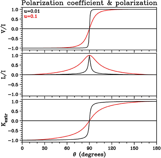
Figure 1. Dependence of the extraordinary mode polarization coefficient, K, as well as of the fraction of linear (L/I) and circular (V/I) polarization, on the angle between the magnetic field and the line of sight, at the limit of small υ and for two values of u.

The conditions for QL propagation are (Zheleznyakov, 1970):

$\begin{array}{ll}\frac{u{sin}^4\theta }{4{cos}^2\theta }<<{(1-\upsilon )}^2,|1-\sqrt{u}cos\theta |>>\frac{(1+\upsilon )usin\theta }{2(1-{\upsilon }^2)}& (10)\end{array}$

which lead to the approximate expressions:

$\begin{array}{ll}{n}_j=1-\frac{\upsilon }{1\mp \sqrt{u}|cos\theta |}& (11)\end{array}$

$\begin{array}{ll}{K}_j=\mp |cos\theta |/cos\theta & (12)\end{array}$

The QT propagation holds when

$\begin{array}{ll}\frac{u{sin}^4\theta }{4{cos}^2\theta }>>{(1-\upsilon )}^2,{tan}^2\theta >>1+\upsilon & (13)\end{array}$

and in this case:

$\begin{array}{ll}{n}_1\simeq 1-\frac{\upsilon (1-\upsilon )}{1-\upsilon -u{sin}^2\theta },n_2\simeq 1-\upsilon & (14)\end{array}$

$\begin{array}{ll}{K}_1\simeq -\frac{(1-\upsilon )cos\theta }{\sqrt{u}},K_2\simeq -\frac{\sqrt{u}}{(1-\upsilon )cos\theta }& (15)\end{array}$

It is important to note that the polarization of the two modes depends only on the properties of the medium in which they propagate and not on the emission mechanism. Therefore, the polarization characteristics are expected to change along the path of the waves, reflecting the local values of the plasma parameters u and υ as well as the angle θ. This is true as long as the geometrical optics approximation is valid, where the two modes propagate independently of each other (weak coupling) and each mode retains its identity as it propagates toward the observer. There is, however, a region along the path where the coupling of the modes becomes strong and the polarization characteristics lock and change no further; this leads to the concept of limiting polarization.

The observed polarization of the radio emission is determined by two factors: (a) the intensity difference between the oppositely polarized extraordinary and ordinary modes, (T_b,1 − T_b,2, in terms of brightness temperature) and (b) the conditions of propagation until the region of limiting polarization is reached. As a consequence, the observed polarization can be quite different from that at the source, in particular if the orientation of the magnetic field reverses along the line of sight.

Going back to the concept of limiting polarization we note that for QL propagation, the condition for strong coupling is (Cohen, 1960; Zheleznyakov, 1970; Bandiera, 1982):

$\begin{array}{ll}C\simeq \frac{1}{2\pi }\frac{1}{\upsilon }{tan}^2\theta \frac{\lambda }{L_B}>1& (16)\end{array}$

where C is the coupling coefficient, L_B is the scale of the magnetic field, and λ is the wavelength. Substituting numerical values we conclude that strong coupling occurs for very low values of density, thus coupling is not expected to affect the observed polarization in the QL case. Much more important is the case of QT propagation, which will be treated in section 6.

3. Free-Free Emission

3.1. Circular Polarization Measurements

Free-free (f-f, bremmstrahlung, see review by Nindos, 2020 in this special research topic collection; see also Gelfreikh, 2004) is the principal emission mechanism for thermal plasma in the absence of gyroresonance emission ($\sqrt{u}\ne 1$, 1/2, 1/3, 1/4,...). The absorption coefficient, k_j, is slightly different for the two wave modes and, in the QL approximation, is given by:

$\begin{array}{ll}{k}_j=\frac{k}{{(1\mp \sqrt{u}\mid cos\theta \mid )}^2}& (17)\end{array}$

where k is the absorption coefficient in the unmagnetized case, given by the well-known approximate expression (e.g., Kundu, 1965)

$\begin{array}{ll}{k}_j(T_e,N_e)=\xi \frac{N_e^2}{n_j{f}^2{T}_e^{3/2}}& (18)\end{array}$

where ξ depends upon the collision frequency and is a slowly varying function of the electron temperature, T_e, and the electron density, N_e; its approximate value is ξ ≃ 0.11 in the chromosphere and ξ ≃ 0.16 in the corona (for a more detailed expression see the review by Nindos, 2020 in this special research topic collection). Note that, as pointed out by Chambe and Lantos (1971), for more accurate computations the term $N_e^2$ should be replaced by $N_e\sum _i{N}_i{z}_i$, where N_i and z_i are the ion density and charge and the sum is over all ions; this, for a H/He atmosphere, will increase the value of ξ to 0.14 in the chromosphere and 0.20 in the corona.

Equation (17) implies that the opacity of the plasma in ordinary radiation will be slightly less than that in the extraordinary, hence the ordinary mode emission will come from lower layers of the atmosphere. If the temperature increases with height, i.e., if the radiation is formed above the temperature minimum, as is the case with solar radio emission, the net effect will be weakly polarized emission in the sense of the extraordinary mode. This is a powerful diagnostic of the magnetic field, because we can immediately obtain qualitative information. Polarized emission reveals the presence of magnetic field and its sense gives the direction of the field with respect to the line of sight: right hand circular polarization corresponds to positive magnetic field, left hand circular to negative. We should note however that, far from the center of the disk, the observed circular polarization may be influenced by propagation effects, as we will discuss in section 6.

Quantitative magnetic field information is harder to extract. The simplest case is that of an optically thin uniform slab (cloud model, see Equation 11 in the review of Alissandrakis, 2020 on the solar atmospheric structure in this special research topic collection) above a uniform background. In this case the brightness temperature, T_bj, will be:

$\begin{array}{ll}{T}_{bj}=T_{bo}{e}^{-{\tau }_j}+T_e(1-e^{-{\tau }_j})\simeq T_{bo}(1-{\tau }_j)+{\tau }_j{T}_e& (19)\end{array}$

where T_bo is the background brightness, T_e the electron temperature and τ_j the optical thickness of the slab (τ_j ≪ 1 for an optically thin slab). In terms of Stokes parameters I (total intensity, here measured above the background) and V (circular polarization) we have:

$\begin{array}{ll}I=\frac{1}{2}(T_{b,1}+T_{b,2})-T_{bo}=({\tau }_1+{\tau }_2)(T_e-T_{bo})& (20)\end{array}$

$\begin{array}{ll}V=\frac{1}{2}(T_{b,1}-T_{b,2})=({\tau }_1-{\tau }_2)(T_e-T_{bo})& (21)\end{array}$

and the fractional polarization, ρ, is:

$\begin{array}{ll}\rho =\frac{V}{I}\simeq \frac{{\tau }_1-{\tau }_2}{{\tau }_1+{\tau }_2}=\frac{k_1-k_2}{k_1+k_2}=2\sqrt{u}cos\theta & (22)\end{array}$

Substituting numerical values, Equation (22) gives for the longitudinal component of the magnetic field:

$\begin{array}{ll}Bcos\theta \left[\text{G}\right]\simeq 5400\frac{\rho }{\lambda \text{[cm]}}& (23)\end{array}$

Thus a 10% polarization at λ = 5 cm requires a magnetic field of 110 G, while at λ = 1 cm the required strength is 540 G. An example is given in Figure 2 which shows I and V images of a facular region obtained with the Nobeyama Radioheliograph (NoRH), together with an MDI magnetogram. We note immediately that the sense of the circular polarization corresponds to the sign of the longitudinal component of the photospheric magnetic field. Moreover, the peak values of V are ~ ±90 K while I is ~ 4, 300 K above the background. Using Equation (23), we obtain a magnetic field in the range of ±100 G, which compares rather well to the photospheric values which are in the range of ±350 G, taking into account the lower resolution of the NoRH and the higher altitude of formation of the radiation at 17 GHz. Note that the NoRH does not have the necessary resolution to reveal the small scale magnetic field associated with the chromospheric network, while high resolution observations (e.g., Bastian et al., 1996) with the Very Large Array (VLA) have not been capable of detecting the relatively low polarization signal. Still, in a recent work, Bogod et al. (2015) reported polarization of 1.4–7% and magnetic field in the range of 40–200 G from RATAN-600 observations of the quiet Sun.

FIGURE 2

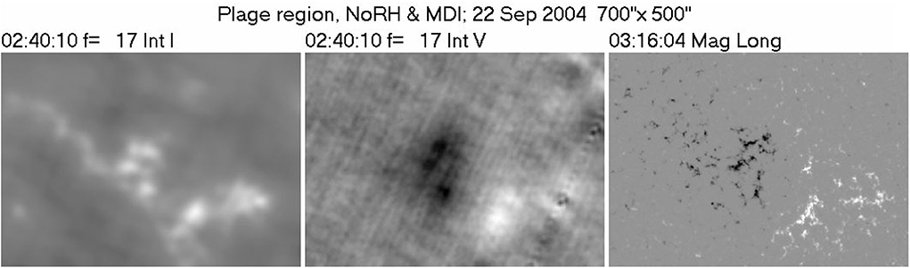
Figure 2. Nobeyama radioheliograph (NoRH) images of a facular region at 17 GHz, in Stokes I (left) and V, (middle) together with an MDI magnetogram (right). The NoRH images are full day averages. This region is located near the central meridian in the images shown in Figure 3. Images produced by the authors.

Things are more complicated in the general case, where physical conditions vary with height. If spectral observations are available, one can use the approximate expression obtained by Bogod and Gelfreikh (1980) (see also Grebinskij et al., 2000) to estimate the longitudinal component of the magnetic field, B_ℓ:

$\begin{array}{ll}{B}_{\ell }\simeq 107\frac{\rho [\%]}{a\lambda [cm]}& (24)\end{array}$

where a is the spectral index:

$\begin{array}{l}a=-\frac{\text{ln }{T}_b}{\text{ln }f}(25)\end{array}$

This expression allows for temperature variations in the region of formation of the radiation and its validity is not limited to the optically thin case, but it implicitly assumes constant magnetic field. Using this method, the above authors estimated the magnetic field above a plage to be about 40 G.

Polarization measurements are scarce beyond the cm-λ range. Using RATAN-600 data, Borovik et al. (1999) measured the circular polarization of an isolated equatorial coronal hole and reported values in the range of 0.2% at λ = 9 cm to 3–4% at 30 cm; using Equation (24), they deduced magnetic field values from ~ 2 G at 2 cm to ~ 10 G at 9 cm, a rather surprising result since one would expect the magnetic field to decrease with height and, hence, with λ. At still longer wavelengths, Ramesh et al. (2010) reported ~ 10% and ~ 15% circular polarization at 109 and 77 MHz, respectively (1.5 and 1.7 R_⊙), from Gauribidanur data. They attributed the emission to coronal streamers and estimated field values of 5 and 6 G. Recently, McCauley et al. (2019) measured the polarization of coronal holes and reported values up to 5–8%, but they made no estimates of the magnetic field.

3.2. Faraday Rotation of Celestial Sources

At larger angular distances from the Sun, the magnetic field of structures in the corona and the solar wind can be estimated from the Faraday rotation of linearly polarized celestial radio sources (Spangler, 2005; Bird, 2007). The position angle of the polarization changes by:

$\begin{array}{ll}\Delta \chi =\frac{e^3}{2\pi m_e^2{c}^4}{\lambda }^2{\displaystyle {\int }_{LOS}{N}_e}\text{B }·\text{ ds}& (26)\end{array}$

where λ is the observing wavelength and ds the path increment along the line of sight (LOS); this expression contains information both about the magnetic field B and the electron density N_e that has to be untangled (see e.g., Kooi et al., 2014).

Ingleby et al. (2007) reported that the magnitude of the coronal field necessary to reproduce the majority of their Faraday rotation observations was in the range of 46–120 mG, at a reference heliocentric distance of 5 R_⊙; however, they could not definitively associate their measurements with any specific coronal structures. Mancuso and Garzelli (2013) used white-light coronograph data to compute the electron density distribution along the line of sight and concluded that, the radial magnetic field, B_r, as a function of the heliocentric distance, R, could be approximated by:

$\begin{array}{ll}{B}_r=3.76{\left(\frac{R}{R_{\odot }}\right)}^{-2.29}[\text{G}]& (27)\end{array}$

for heliocentric distances from about 5 to 14 R_⊙; this gives 94 mG at 5 R_⊙. Kooi et al. (2017) also used white-light information and deduced fields of ~ 11 mG for two CMEs located at heliocentric distance of around 10 R_⊙ and 2.4 mG for a jet-like CME at ~ 8 R_⊙.

Faraday rotation measurements of interplanetary space probe signals, such as Helios (e.g., Pätzold et al., 1987; Efimov et al., 2015) and MESSENGER (e.g., Wexler et al., 2019) can provide information on the magnetic field lower in the corona, but this information is highly dependent on electron density models and variations of the magnetic field in the region of closest solar approach. Pätzold et al. (1987) deduced the following relation:

$\begin{array}{ll}{B}_r=\left(\frac{6}{R^3}+\frac{1.18}{R^2}\right) [\text{G}]& (28)\end{array}$

valid for R between 2 and 9 solar radii. Wexler et al. (2019) quote values of 1,000–12,000 nT (10–120 mG) at 1.61 R_⊙.

4. Gyroresonance Emission

Gyroresonance (g-r) emission is produced by thermal electrons gyrating around the lines of force of the magnetic field. It is strong in regions where the observing frequency, f, is a low order harmonic (2nd to 4th) of the electron gyrofrequency, ω_ce = eB/m_ec; thus, for a given harmonic s, the following numerical relation holds between the wavelength of observation and the magnetic field:

$\begin{array}{ll}B[G]=\frac{10700}{s\lambda [\text{cm}]}=\frac{360f[\text{GHz}]}{s}& (29)\end{array}$

Consequently a fairly high magnetic field is necessary (e.g., 600 G for third harmonic emission at 6 cm-λ). Although gyroresonance radiation is emitted at discrete frequencies, it generally gives rise to a continuous spectrum due to the variation of the magnetic field with height; there are some exceptions to this, as will be discussed in section 4.2.

4.1. The Magnetic Field Above Sunspots

Due to their high magnetic field strength, sunspots are an obvious place to look for gyroresonance emission; historically, sources of localized microwave emission were discovered first (Kundu, 1959) and then the emission mechanism was identified (Kakinuma and Swarup, 1962; Zheleznyakov, 1962). The emission is generated in thin layers around iso-Gauss surfaces where the magnetic field strength is such that the observing frequency is equal to a harmonic of the local gyro-frequency; the surfaces of harmonic layers are nicely displayed in Figure 8 of Lee (2007).

The close association of the g-r emission to the magnetic field, makes it a valuable tool for the study of the atmospheric layers above sunspots and for magnetic field measurements (e.g., Gelfreikh, 1998). This has stimulated a large amount of theoretical and observational work over a long period of time, particularly after the first high resolution observations by Kundu and Alissandrakis (1975) and the first detailed modeling by Alissandrakis et al. (1980). Recent works are reviewed by White (2004) and Lee (2007). High-resolution multi-wavelength observations of sunspots can be used to test in detail models of magnetic field extrapolation from measurements at the photosphere (Lee et al., 1998a). In general, observations and modeling can provide valuable diagnostics of the active region atmosphere and magnetic field, in particular if high spatial resolution spectral data are available (e.g., Tun et al., 2011; Nita et al., 2018; Stupishin et al., 2018; Alissandrakis et al., 2019a).

The g-r opacity (Kakinuma and Swarup, 1962; Zheleznyakov, 1962) is a complicated function of the temperature, the density, the intensity of the magnetic field, the wave mode and has a strong dependence on the direction of the field with respect to the line of sight, being zero when these are parallel. It is much greater in the extraordinary mode than in the ordinary, it is also much greater at the second harmonic than at the third; thus, under conditions prevailing in the sunspot atmosphere, in the microwave range the third harmonic is usually opaque in the extraordinary and transparent in the ordinary mode, while the second harmonic is opaque in both modes. Emission from the fundamental is not expected, because it is obscured by the overlying second harmonic layer, while emission at the fourth harmonic can appear at long cm wavelengths (Kaltman and Bogod, 2019).

Measurements of the magnetic field can be obtained without resorting to detailed modeling. We note that if the photospheric field is weak enough (or the frequency is high enough) both the 3rd and the 2nd harmonic layers are below the Transition Region and no strong sunspot-associated emission is expected. For stronger field, or lower frequency, the third harmonic enters into the TR while the second is still in the chromosphere; consequently strong emission is observed, highly polarized in the sense of the extraordinary mode (e.g., Shibasaki et al., 1994). For still higher field strength, the second harmonic also enters the TR; we then have strong emission in the ordinary mode as well as in the extraordinary and the polarization is reduced. Thus, the brightness temperature spectrum of both I and V show a rapid rise at the wavelength where the third harmonic enters into the TR; the magnetic field at the base of the TR can be estimated from the extrapolation of V to zero and the expression (29) with s = 3 (Akhmedov et al., 1982). Such measurements are routinely made from RATAN-600 data and are available at http://www.sao.ru/hq/sun/.

The appearance of gyroresonance sources is illustrated in Figure 3, which shows radio images of a bipolar active region, obtained by the NoRH and the Siberian Solar Radio Telescope (SSRT), together with a photospheric magnetogram. The photospheric magnetic field is ~ −3,000 G at the leading sunspot and ~ 1, 600 G at the trailing. There is no trace of sunspot-associated emission at 34 GHz, which means that the 3rd harmonic layer (4,050 G) is below the base of the TR. At 17 GHz we have strong emission from the leading spot in the extraordinary mode (left circular polarization) and no emission in the ordinary mode, which means that the third harmonic level (2,025 G) is already in the low TR; at the same frequency there is no o-mode emission from the leading sunspot, i.e., the second harmonic level (3,040 G) is still below the TR. At 5.7 GHz there is strong emission both in the L and R sense, from which we may deduce that both the second (1,020 G) and third (680 G) harmonics are above the base of the TR. On the basis of this information, and the fact that, when an harmonic layer is opaque, the observed brightness temperature is equal to the local electron temperature, one can reconstruct roughly the variation of the magnetic field strength as a function of temperature (Figure 4, left). This is a peculiar magnetogram, in the sense that the temperature, rather than the height plays the role of the independent variable.

FIGURE 3

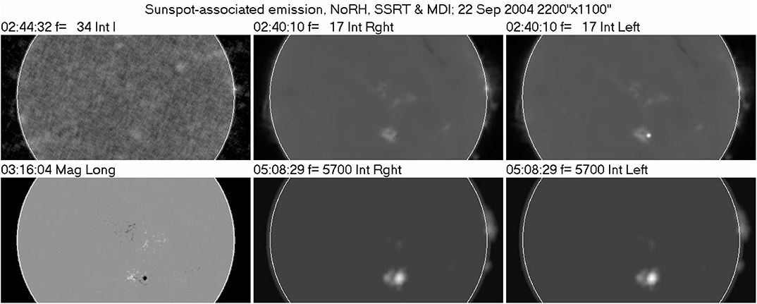
Figure 3. Radio images of an active region. (Top) NoRH (34 GHz, Stokes I and 17 GHz, R and L polarization). (Bottom) MDI magnetogram and SSRT images (5.7 GHz, R and L polarization). White arcs show the photospheric limb. Images produced by the authors.

FIGURE 4

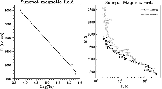
Figure 4. (Left) The variation of the magnetic field strength with temperature for the leading sunspot of Figure 3. (Right) A similar plot obtained from RATAN-600 spectral data, adapted from Korzhavin et al. (2010); open and filled triangles show results from ordinary and extraordinary mode data, respectively.

More detailed information can be obtained if spectral, rather than single frequency observations are available, such as with the RATAN-600 radio telescope. The right panel of Figure 4 shows results obtained by Korzhavin et al. (2010). A shortcoming of this method is that, at some wavelengths, both the second and the third harmonic may contribute to the emission in the extraordinary or ordinary mode, as shown by model computations (Alissandrakis et al., 1980).

In order to obtain the magnetic field as a function of height, one has to use a temperature-height model; this, however, is not necessary if the height of the radio emission could be measured by other means. Using a stereoscopic method to measure the height, Bogod et al. (2012) presented results for a number of stable sunspots and compared them with extrapolations of the photospheric magnetic field; they found several cases where the magnetic field intensity measured in this way was greater than the extrapolated one. There have been other indications that the magnetic field above sunspots is rather high; Akhmedov et al. (1982) reported values 80–90% of the photospheric field at the base of the TR, while Brosius and White (2006) reported coronal magnetic field strengths of 1,750 G at a surprisingly large height (8,000 km) above a large sunspot at the west solar limb. In a recent work, Anfinogentov et al. (2019) reported g-r emission at 34 GHz from NoRH data, indicating a magnetic field of at least 4,050 G at the base of the TR; this was associated to a sunspot with a photospheric field above 5,000 G.

Under certain circumstances it is possible to derive not only the magnitude of the magnetic field, but also its orientation. The gyroresonance absorption coefficient has a very strong angular dependence and becomes zero when the magnetic field is parallel to the line of sight. Thus, on a sunspot associated source, there will be a region of low intensity at the location where this condition is fulfilled. This region will be very small (below the instrumental resolution) for x-mode emission but it can be observed in o-mode. Consequently, at that location we will have lower than average intensity and high circular polarization. Alissandrakis and Kundu (1984), using observations with the WSRT were able to identify this low intensity region over a stable sunspot and, using images over six consecutive days, to measure the inclination of the magnetic field as a function of distance from the sunspot center (Figure 5).

FIGURE 5

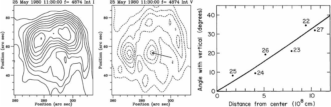
Figure 5. Intensity and polarization maps of a stable sunspot, observed with the Westerbork Synthesis Radio Telescope (WSRT) on May 25, 1980. The arrow points to the region of low intensity and high polarization near the center of the sunspot, where the magnetic field is parallel to the line of sight (from data used in Alissandrakis and Kundu, 1984). The right panel shows the derived inclination of the magnetic field as a function of distance from the sunspot center; data points are marked with the date of observation (May 1980) and the full line is the expected inclination for a force-free field model. From Alissandrakis and Kundu (1984), reproduced with permission © ESO.

4.2. Cyclotron Lines

As mentioned in section 4.1, the observed spectrum of gyroresonance emission is continuous due to the height variation of the magnetic field. This is true as long as the magnetic field decreases monotonically with height and the electron temperature increases, as is the case above the photosphere of sunspots. However, as pointed out by Zhelezniakov and Zlotnik (1980), if there is a hot structure in the corona (e.g., a hot loop) as shown in the left panel of Figure 6, the emission at the frequency corresponding to the third harmonic for the value of the magnetic field at the hot structure will be higher than that of nearby frequencies, giving rise to a cyclotron line. The width of the line will depend on the extent of the hot structure and the gradient of the magnetic field, while its polarization will be that of the extraordinary mode if, as expected, τ_x > 1 and τ_o < 1. At the frequency corresponding to the second harmonic the emission will be polarized in the sense of the ordinary mode, because the extraordinary mode will be obscured by the 3rd harmonic layer which is located higher.

FIGURE 6

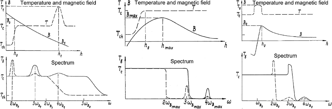
Figure 6. Three configurations that can produce cyclotron lines: A hotter than average structure in the corona (left), a maximum in the magnetic field (middle), and a hot current sheet (right). The top panels show the variation with height of the electron temperature and the magnetic field, bottom panels the expected brightness temperature spectrum in the extraordinary (full lines) and ordinary (dashed lines) mode. T_ch is the electron temperature of the chromosphere, T_c of the corona and T_t of the hot structure. Adapted from Zhelezniakov and Zlotnik (1980).

Two more configurations that produce cyclotron lines are shown in Figure 6. A peak in the magnitude of the magnetic field, as shown in the middle panel, will result in excess o-mode emission near the 3rd harmonic and x-mode emission near the 4th. The bandwidth of the line will be (Zhelezniakov and Zlotnik, 1980):

$\begin{array}{ll}\frac{\delta f}{f}=\sqrt{2}{\beta }_{T}cos\alpha & (30)\end{array}$

where β_T is the ratio of the thermal electron velocity to the velocity of light and α is the angle between the magnetic field and the line of sight. A current sheet, providing at the same time an inversion of the sign of the magnetic field and energy release to locally heat the corona (Figure 6, right panel) will lead to excess emission at the 4th, 3rd, and 2nd harmonics.

It is obvious from the above that cyclotron lines provide a direct measurement of the value of the magnetic field at the location where they are formed while, at the same time, they reveal the particular conditions of their formation, since each case presented above has its own spectral signature.

Cyclotron line detection requires spectrally resolved imaging observations at closely spaced frequencies, with adequate stability of the instrumental gain, thus observational evidence has been scarce: Willson (1985) reported an unpolarized spectral feature with a brightness temperature excess of a factor of ~2.5 and a spectral width of δf/f ~ 0.1, in VLA observations at ten frequencies near 20 cm (1,440–1,724 MHz). His interpretation was in terms of a hot loop with a constant magnetic field of ~145 G for emission at the 4th harmonic. These results were re-analyzed by Zhelezniakov and Zlotnik (1989), in a more realistic approximation of inhomogeneous magnetic field; they obtained a better fit to the data, with emission at the 3rd harmonic (B = 196 G). The absence of polarization was attributed to the high optical thickness of both modes and the spectral width to the variation of the magnetic field. A similar case, again observed with the VLA at the same frequencies, was reported by Lang et al. (1987) and also interpreted in terms of a hot loop.

Evidence of cyclotron lines has been found in 1-dimensional spectral observations with the RATAN-600 radio telescope. A narrow, polarized spectral feature was reported by Bogod et al. (2000) near 8.5 cm, possibly associated with a compact bright source observed at 17 GHz with the Nobeyama radioheliograph. The lack of any other line in the observed spectral range led the authors to identify it with 3rd harmonic emission, implying a magnetic field of ~400 G; the derived parameters were further constrained by assuming that the 17 GHz source was due to thermal f-f emission from the same hot structure. We should note at this point that peculiarities in spectra, such as a broad minimum in both I and V have been reported by Yasnov et al. (2011) and interpreted using a model with a hot coronal loop.

5. Gyrosynchrotron Emission

The characteristics of gyrosynchrotron (g-s) emission from mildly relativistic electrons, trapped in flaring loops, depend strongly on the magnetic field (see the review by Nindos, 2020 in this special research topic collection and the reviews by Bastian et al., 1998 and Nindos et al., 2008). The emission has a quasi-continuous spectrum with maximum in the low harmonics of the gyrofrequency. The peak wavelength of the observed intensity spectrum is mainly determined by opacity effects (self absorption), which shift the peak to the 3rd–4th harmonic (Takakura, 1967). Thus a spectral maximum at 6 cm corresponds to magnetic field strength of 450–600 G; the field is obviously higher in bursts with spectra that peak at shorter wavelengths, sometimes in the millimeter range.

It should be noted that the magnetic field in burst sources is highly inhomogeneous, thus these values should be considered as gross estimates only. Detailed model computations of g-s emission from a homogeneous distribution of energetic electrons in a flaring loop by Preka-Papadema and Alissandrakis (1988) showed that the spectral peak can occur between the second and sixth harmonic; the spectral maximum shifts to shorter wavelengths as we move from the top of the loop to its footpoints, as a result of the variation of the magnetic field strength and direction. Moreover, the emission is expected to peak at the top of the flaring loop in the optically thick case and at the footpoints in the optically thin. Subsequent model computations have treated inhomogeneous and anisotropic distributions of non-thermal electrons, as well as time variations (Fleishman and Melnikov, 2003; Tzatzakis et al., 2008; Simões and Costa, 2010; Nita et al., 2015).

It is obvious from the above discussion that the use of g-s emission for diagnostics of the magnetic field is not as straight forward as in the case of gyroresonance. For reliable diagnostics one requires data with high spatial, spectral, and temporal resolution (i.e., dynamic imaging spectroscopy), as the spectrum will vary from point to point and as a function of time. Homogeneous source models, as well as simplified expressions for the emission are not expected to produce satisfactory results. Simultaneous hard X-ray data are useful in providing independent information about the energy distribution of the accelerated electrons. The observations should be combined with models of all physical parameters that influence the emission, including the magnetic field. In the past, any information on the magnetic field came as a byproduct of the modeling, and not as a more or less direct measurement.

In spite of the difficulties, some results from detailed modeling of observations have been reported. Using VLA I and V images at 5 and 15 GHz and spectral data from the Owens Valley Radio Observatory at several frequencies between 2 and 15 GHz, Nindos et al. (2000) deduced a magnetic field strength of 870 G at the feet and 270 G at the top of a flaring loop. Values in the same range (1,700–200 G) were obtained from Nobeyama images at 17 and 34 GHz by Kundu et al. (2001, 2004), Tzatzakis et al. (2008), and Kuznetsov and Kontar (2015).

The Expanded Owens Valley Solar Array (EOVSA) has provided a breakthrough for measuring magnetic fields and other parameters of flares using g-s emission, by providing high-cadence, spatially-resolved spectra permitting direct spectral fitting. A limb flare was among the first results from EOVSA; images at 30 frequencies from 3.4 to 18 GHz were analyzed by Gary et al. (2018) and preliminary field values from 150 to 520 G were derived. A more thorough analysis of the EOVSA data during the main phase of the event by Fleishman et al. (2020) has provided the first maps of the dynamically decaying magnetic field strength in the cusp region of a flare. Additionally, the magnetic field vs. height along the reconnecting current sheet of the early, eruptive stage of the flare was measured and compared with an MHD simulation by Chen et al. (2020).

An important application of g-s emission is in the measurement of the magnetic field in Coronal Mass Ejections (CME), provided that this mechanism rather than plasma emission is the dominant radiation mechanism of the associated type IV metric radio bursts (see also Vourlidas et al., 2020 in this special research topic collection). This distinction can be made on the basis of the low brightness temperature and the spectral shape, which shows a characteristic peak (Klein and Trottet, 1984; see examples in Figure 7). Radio CMEs are rare; among the early works, Gopalswamy and Kundu (1987) estimated a magnetic field of ~2 G at heliocentric 2.3 R_⊙. Subsequent works (Bastian et al., 2001; Maia et al., 2007; Tun and Vourlidas, 2013; Bain et al., 2014; Carley et al., 2017; Mondal et al., 2020) gave a range of values between 0.3 and 23 G in the heliocentric distance range of 1.3–2.7 R_⊙, which variation apparently pertains to individual CMEs rather than to the ambient corona. Moreover, all authors used homogeneous source models and simplified expressions for the g-s emissivity.

FIGURE 7

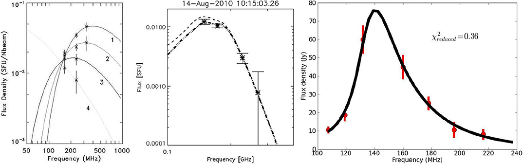
Figure 7. Examples of radio CME spectra and model fits. (Left) from Bastian et al. (2001); (middle) from Tun and Vourlidas (2013); (right) from Mondal et al. (2020). All panels reproduced by permission of the AAS.

6. Circular Polarization Inversion

We already mentioned in section 3 that, as the physical conditions change along the ray path, the polarization of electromagnetic waves changes accordingly. Consequently, the observed polarization will not be the same as the polarization at the region of formation of radiation. In particular, if the wave crosses a transverse field region (TFR), where the magnetic field is perpendicular to the line of sight, the sense of its polarization will change, since the sign of the longitudinal component of the magnetic field changes. This happens as long as the geometrical optics approximation is valid, i.e., for not too low values of N_e and B. In a more general sense, the situation is described in terms of wave coupling. When the coupling between the x-mode and o-mode waves is weak their polarization properties change along the ray path, whereas when the geometrical optics approximation breaks down the waves are strongly coupled and their polarization remains fixed, even if a TFR is crossed.

The most prominent effect of wave propagation is the inversion of circular polarization as a bipolar active region moves from the eastern to the western limb (Alissandrakis, 1999; Ryabov, 2004). In this section we will discuss how this effect can provide information on the magnetic field in the low corona above active regions.

6.1. Wave Coupling Under QT Propagation

Wave coupling has been studied comprehensively by Cohen (1960) (see also Bandiera, 1982; Zheleznyakov et al., 1996; Segre and Zanza, 2001). In the case of QL propagation, the coupling becomes strong for extremely low values of the density (section 3). Of more practical interest is the case of QT propagation; in this case the coupling coefficient is:

$\begin{array}{ll}C=a\frac{{\omega }^4}{N_e{B}^3}\left|\frac{d\theta }{ds}\right|& (31)\end{array}$

where

$\begin{array}{ll}a=\frac{2\text{ ln }2}{{\pi }^2}\frac{m_e^4{c}^4}{e^5}& (32)\end{array}$

and the symbols have their usual meaning.

Taking into consideration the effect of wave coupling, the sense of circular polarization does not necessarily change when the waves cross a TFR. In fact, what happens depends on the value of C at the point, along the ray path, where the longitudinal component of the magnetic field, B_ℓ, vanishes:

• If C ≪ 1 the polarization changes sense (weak coupling)

• If C = 1 the polarization becomes linear (critical coupling)

• If C ≫ 1 the sense of polarization does not change (strong coupling)

Of particular interest is the case of C ≈ 1, which has been treated by Zheleznyakov and Zlotnik (1963). After the TFR crossing, the resulting polarization is elliptical, with the degree of circular, ρ_c, and linear, ρ_ℓ polarization given by:

$\begin{array}{ll}{\rho }_c=-1+2exp\left(-\frac{\text{ln }2}{C}\right)& (33)\end{array}$

$\begin{array}{ll}{\rho }_{\ell }=2exp\left(-\frac{\text{ln }2}{2C}\right)\sqrt{1-exp\left(-\frac{\text{ln }2}{C}\right)}& (34)\end{array}$

which, for C = 1 give ρ_c = 0 and ρ_ℓ = 1; note that ρ_c = −1 for C ≪ 1, while ρ_c = 1 for C ≫ 1; at both limits ρ_ℓ = 0 (Figure 8, top row).

FIGURE 8

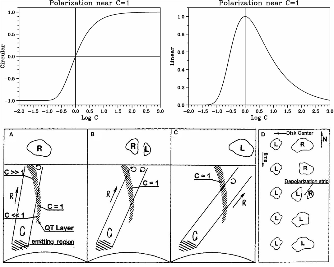
Figure 8. (Top) Circular (left) and linear (right) polarization after TFR crossing, as a function of the coupling coefficient. (Bottom) Geometry of radiation crossing a transverse field region (QT layer); (A–C) Polarization inversion of the limbward part of an active region as it rotates from the disk center to the west limb; (D) effect on a bipolar active region. (after Bandiera, 1982, reproduced with permission © ESO).

We note here that, with the continuum receivers typically used in past radio observations, the observation of linearly polarized radiation from the Sun was not possible, due to the strong Faraday rotation within the receiver bandwidth. Further difficulties may arise from wave scattering in coronal inhomogeneities (Bastian, 1995). In spite of these difficulties, Alissandrakis and Chiuderi-Drago (1994) reported the detection of linearly polarized radiation and measured the Faraday rotation, using a narrow band (Δf/f = 4 × 10⁻⁶) spectral line receiver. From their observations, Segre and Zanza (2001) deduced a magnetic field of 12.8–11.2 G and a value of 1.40–2.08 × 10¹⁸ cm⁻² for the product of electron density and the magnetic field scale. It should be noted that due to advances in high-speed signal processing modern radio receivers now routinely provide sufficient spectral resolution to renew interest in the detection of linear polarization. For example, EOVSA has a special narrow-band mode that provides Δf/f = 6 × 10⁻⁵ at 10 GHz, while the Very Large Array can achieve Δf/f = 5 × 10⁻⁴ at 8 GHz.

Even if linear polarization cannot be detected, we can still make use of frequency-dependent spatial patterns in circular polarization to locate the TFR. Let us note from the beginning that normally only a source located in the limbward part of an active region may suffer polarization inversion, simply because radiation from the diskward part will not cross a TFR. Consider now such a source emitting right circularly polarized radiation, which crosses a TF region on its way to the observer (Figure 8, bottom). When the source is near the disk center (Figure 8 bottom, A), the TFR is crossed high in the corona where the density and the magnetic field are low and the coupling strong, after Equation (31); consequently the observed polarization is the same as the intrinsic. As the region moves toward the West limb (Figure 8 bottom, B), the radiation crosses the TFR at a lower height, hence the coupling coefficient decreases; at a certain point the radiation from the east part of the source will cross the TFR under conditions of weak coupling, and the sense of its circular polarization will be inverted. Closer to the limb (Figure 8 bottom, C), the radiation from the entire source will cross the TFR under weak coupling conditions and the observer will see left rather than right circular polarization.

The resulting polarization map of the entire bipolar active region as it moves from the disk center to the west limb, including the unreversed diskward side, is sketched in Figure 8 bottom, D. The left and right circularly polarized components are separated by the depolarization strip, i.e., a region of low circular polarization between the two oppositely polarized sources, which will be displaced with respect to the photospheric neutral line (where B_ℓ = 0) by an amount which increases as the active region moves toward the limb. Furthermore, the displacement is a function of frequency, generally being larger at lower frequencies although it depends on the detailed shape of the TFR (C = 1 layer sketched in Figure 8, bottom; e.g. Ryabov, 2004). For a region in the Eastern hemisphere the situation is the reverse: near the limb the observed sense of circular polarization will correspond to the leading magnetic polarity.

6.2. Observations

The inversion of circular polarization in the radio emission of active regions and bursts has been known for several years (Kundu, 1965; Zheleznyakov, 1970). In low resolution observations of active regions where the two polarities are not resolved, the total V is in the sense of the magnetic polarity of the leading part of the region when the source is located in the eastern hemisphere, while the polarization is in the sense of the trailing polarity when the source is in the western hemisphere (e.g., Peterova and Akhmedov, 1974). The effect is better illustrated in high resolution two-dimensional data. An example observed with the WSRT at 6 cm in 1980 is shown in the top four rows of Figure 9. Notice that on June 13 (top row), when the Active Region was in the Eastern hemisphere, its trailing part is depolarized; the bipolar structure of the magnetic field is fully revealed on June 16 (fourth row), after the central meridian crossing. Another example, this time from RATAN-600 1-D scans, is shown in the bottom four rows of Figure 9; here V is fully inverted in the trailing part of the active region near the E limb (left column) and in the leading part near the W limb (right column).

FIGURE 9

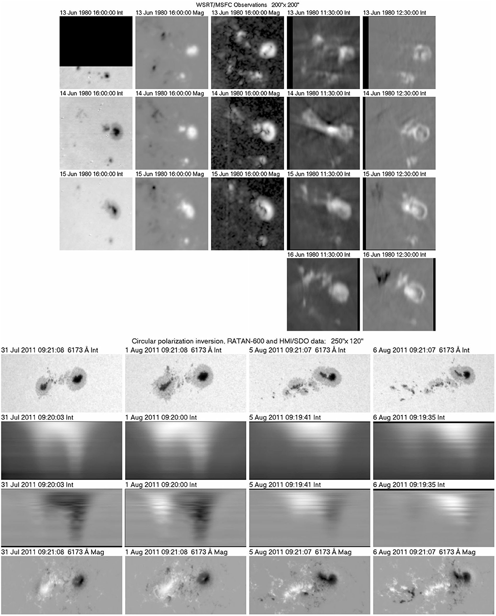
Figure 9. Rows 1–4: WSRT observations of two active regions in total intensity (fourth column) and circular polarization (fifth column), together with white light photographs (first column) and magnetograms (longitudinal: second column, transverse: third column) from the Marshal Space Flight Center. The region was near the East limb on the first day (first row) and had crossed the central meridian on the last day (fourth row). Right hand circular polarization is white. (Images from data used in Chiuderi Drago et al., 1987). Rows 5–8: An active region crossing the solar disk. Row 5: white light images (HMI). Rows 6–7: RATAN-600 one-dimensional scans in Stokes I and V in the wavelength range 3.65 (bottom of panel) to 8 cm (top of panel). Last row: magnetograms (HMI). The region crossed the central meridian between August 3 and 4. RATAN images constructed from data at ftp://ftp.sao.ru/pub/sun/sun_fits.

The position of the depolarization strip (where V ≃ 0) depends on wavelength. Equation (31) implies that C is higher at short wavelengths, which means that the region of critical coupling moves lower in the corona; as a result the depolarization strip is closer to the photospheric neutral line (where B_ℓ = 0). This is illustrated in the RATAN-600 observations in Figure 9: note that on August 1, as we go from short to long wavelengths, the depolarization strip moves in the direction of the limb (eastward); the same effect is seen on the August 5 scans, the limb now being in the west. We note in passing that g-r emission from the leading spot starts at shorter wavelengths than from the trailing one, due to the stronger magnetic field of the former (section 4.1).

If we consider the spectrum of Stokes V at a point in the limbward part of an active region, we expect inversion to occur at wavelengths longer than a critical value, where C ≥ 1 (note that the coupling coefficient goes like λ⁻⁴, see Equation 31). In a number of cases a second inversion is observed at longer wavelengths (Bogod et al., 1993; Ryabov, 1998). This can be explained by the radiation crossing two TFRs on its way to the observer, something that may happen under complex morphologies of the magnetic field. The first inversion occurs at the wavelength where C = 1 at the lower TFR; in this case the upper TFR will not affect the polarization because the coupling will be strong there, due to the much lower density and field strength. As the coupling decreases with wavelength, the second inversion will occur at longer λ, where both TF regions are crossed under conditions of weak coupling.

Notice that the above discussion is independent of the intrinsic polarization of the wave at the site of its generation. Propagation effects, at longer wavelengths in particular, can change considerably the sense of circular polarization expected on the basis of the emission mechanism. The observations give a picture of the magnetic field polarity not at the source of the emission, but at the height where C = 1. Therefore one should be careful in inferring the polarity of the magnetic field on the basis of V maps, particularly in regions far from the disk center and at long wavelengths. One more point made by Kundu and Alissandrakis (1984) is that, due to the expected smoother geometry of the coronal magnetic field at large heights, small scale magnetic structures should not be detectable on V maps. Another point raised by Alissandrakis and Preka-Papadema (1984) concerns the identification of the magnetic polarity of microwave burst footpoints, which may also be affected by propagation effects (see Alissandrakis et al., 1993).

The crossing of a TFR is not the only known mechanism of polarization inversion. It has been pointed out (e.g., Zheleznyakov et al., 1996) that the geometrical optics approximation is violated and mode coupling occurs also in the case of radiation crossing plasma current sheets with a weak guide field.

6.3. Diagnostics

Several methods for diagnostics of the magnetic field exist; the choice depends on the available data. For example, if two or one-dimensional information at a single frequency is available over several days, the distance, q, of the depolarization strip from the photospheric B_ℓ = 0 line can be measured. Using a dipole approximation for the large scale magnetic field of an active region, Kundu and Alissandrakis (1984) derived the following expression, extending the work of Bandiera (1982):

$\begin{array}{ll}q=-2\beta {\left(\frac{\alpha -\ell }{3}\right)}^{7/8}& (35)\end{array}$

where α is the dipole inclination with respect to the surface, ℓ the longitude, $\beta =(N_e{d}^3)/(6a{\omega }^4)$, a is the constant defined in Equation (32) and d is the dipole magnetic moment. They determined β and α by fitting the data, and from those the height of the critical point and the quantity $N_e{d}^3$. Assuming a reasonable value of N_e they obtained d and furthermore B. The exact value of the electron density is not critical, because the magnetic field is proportional to the cubic root of its value. Their results, together with those of others, are listed in Table 1.

TABLE 1

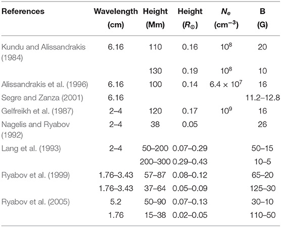
Table 1. Coronal parameters from circular polarization inversion.

Sometimes high resolution data are available for a single day only (Alissandrakis et al., 1996). In this case one can extrapolate the photospheric magnetic field and find the height at which the projection of the B_ℓ = 0 line matches the position of the depolarization strip. The height of the region of critical coupling as well as the magnetic field parameters are obtained from the extrapolation and the electron density can be computed from the condition C = 1. This method, however, does not give a very accurate value of N_e due to its appearance in the third root in the expression, while other uncertainties may arise from the validity of magnetic field extrapolation (Lee et al., 1998b).

Data of V as a function of both the position and the wavelength are readily available thanks to the RATAN-600 radio telescope. The Pulkovo group (e.g., Peterova and Akhmedov, 1974; Gelfreikh et al., 1987; Nagelis and Ryabov, 1992; Lang et al., 1993; Kaltman et al., 2007) have worked extensively with these and some of their results are included in Table 1. Note that the RATAN observations extend to short cm-λ, which allows one to access lower heights and stronger magnetic fields.

The diagnostic methods presented so far are based on measurements of the position of the depolarization line in space and/or in frequency. Additional diagnostics can be developed on the basis of the change of the degree of circular polarization as a function of frequency and position, described by Equation (33) and plotted in the left top panel of Figure 8; this expression determines, e.g., the width of the depolarization strip as well as the rate of change of polarization in the direction perpendicular to the strip. The work of Gelfreikh et al. (1997) is in that direction; they used Equation (33) to determine the gradient of the magnetic field and obtained typical values in the range of 10⁻⁹ G/cm a height of 120 Mm, with a single value as high as 2 × 10⁻⁵ G/cm at a height of 50 Mm.

If the intrinsic polarization of the waves were known, one could use Equation (33) to obtain a map of the coronal magnetic field in the region where C ≈ 1. Ryabov et al. (1999) using observations from the Nobeyama Radioheliograph together with RATAN-600 scans, determined the intrinsic polarization on a day without any obvious inversion and subsequently computed the degree of circular polarization for the next day when inversion was observed; in this way they obtained a coronal magnetogram. This appears to be a very powerful method for magnetic field diagnostics, although it is applicable to a rather limited number of cases. More results were obtained by Ryabov et al. (2005), who used combined NoRH and SSRT observations over several days to deduce field strengths of 30 to 10 G at heights of 50–90 Mm and 110–50 G at the heights of 15 to 38 Mm. Their results are shown in Figure 10.

FIGURE 10

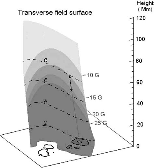
Figure 10. Map of the magnetic field on the transverse field surface above a bipolar active region, deduced from observations of the inversion of circular polarization. Adapted from Ryabov et al. (2005).

The works presented above show an almost perfect agreement between observations and theory. However, cases of disagreement have also been reported, mainly in the long decimetric and metric range (Gopalswamy et al., 1991; White et al., 1992). Efforts have been made to interpret these results in terms of current sheets (Gopalswamy et al., 1994) or scattering in inhomogeneities (Bastian, 1995).

7. Fiber Bursts and Zebra Patterns

Type IV bursts in the metric and decimetric range are rich in fine structures, embedded in the background continuum emission. Among them, fiber bursts and zebra patterns show periodic maxima and minima in their instantaneous flux spectrum (see reviews by Chernov, 2006, 2011; Nindos and Aurass, 2007). In both cases the frequency of the peaks drifts with time: monotonically toward low frequencies in the case of fibers and in a wavy manner in the case of zebra patterns (Figure 11).

FIGURE 11

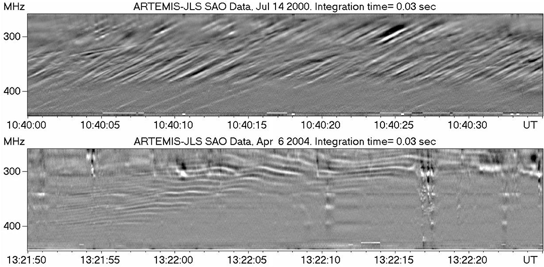
Figure 11. Dynamic spectra of fiber bursts (top) and zebra pattern (bottom), observed with the ARTEMIS/JLS radio spectrograph (Kontogeorgos et al., 2006) in the 266–451 MHz range. The spectra have been filtered in time and frequency to improve the visibility of fine structures. Data selected by C. Bouratzis.

Fiber bursts (also known as intermediate drift bursts, their frequency drift rate being between those of type II and type III bursts), are commonly attributed to the coalescence of whistler and Langmuir waves formed by a loss cone distribution of non-thermal electrons in post-flare loops (see Kuijpers, 1975, also Mann et al., 1987, 1989). As demonstrated with imaging observations by Alissandrakis et al. (2019b), these loops are considerably higher than microwave and soft X-ray burst loops and probably encompass both the low flaring loops and the CME-associated flux rope. According to this interpretation, each fiber is a whistler wave packet propagating upwards in the loop; the group velocity, v_g, is (Kuijpers, 1975):

$\begin{array}{ll}{\upsilon }_g=2{\upsilon }_{Ae}\sqrt{x{(1-x)}^3}=2c\frac{{\omega }_{ce}}{{\omega }_{pe}}\sqrt{x{(1-x)}^3}& (36)\end{array}$

where

$\begin{array}{ll}{\upsilon }_{Ae}=\frac{B}{\sqrt{4\pi N_e{m}_e}}& (37)\end{array}$

is the electron Alfvén velocity, which is about 43 times higher than the usual Alfvén velocity

$\begin{array}{ll}{\upsilon }_A=\frac{B}{\sqrt{4\pi N_e{m}_p}}& (38)\end{array}$

and x = ω_w/ω_ce is the ratio between the whistler frequency and the electron gyrofrequency.

The group velocity can be retrieved from the frequency drift using a density model. According to Equation (36), υ_g maximizes for x = 0.25 and Kuijpers (1975) argued that 0.1 > x > 0.5, so that υ_g is between 21.5 and 28 υ_A; he used this and the drift velocity to estimate magnetic field strengths of 11.5–15 G at the level of formation of the emission at 900 MHz and 0.51–0.66 G at 160 MHz. An additional diagnostic is provided by the whistler frequency, which is expected to be equal to the separation between the emission and absorption ridges of the fiber, since the radiation is enhanced at ω_p + ω_w and reduced at ω_p; taking this into account, Kuijpers (1975) gave field values of 7.2–36 G at 900 MHz and 0.36–1.8 G at 160 MHz. Note, however, that these estimates serve more as a check for the model rather than as magnetic field measurements.

Measurements of the frequency drift and the whistler frequency can be combined, in which case Equation (36) gives:

$\begin{array}{ll}\frac{L_N}{c}\frac{1}{f_w}\frac{df}{dt}=\sqrt{\frac{{(1-x)}^3}{x}}& (39)\end{array}$

which can be solved for x and hence for B. Here the group velocity has been expressed in terms of the frequency drift rate, df/dt; f_w is the whistler frequency and L_N is the density scale height along the magnetic field lines of the loop which must come from model estimates. For the fibers shown in Figure 11, Equation (39) gives 5.6 G at 370 MHz and 4 G at 290 MHz, assuming that L_N = 100 Mm. Additional information can be obtained from the derivative of the frequency drift; in this way, Benz and Mann (1998) obtained 212 G at 2 GHz and 5.7 G at 212 MHz for the whistler model, while they got 143 and 14 G, respectively for an alternative model in which the radiation is produced by maser emission at a harmonic of the electron cyclotron frequency and the fiber modulation by an Alfvénic soliton.

In a more elaborate treatment, Aurass et al. (2005) used 2D positions from the Nançay Radioheliograph, together with potential extrapolations of the photospheric magnetic field and a α × Newkirk density model (Newkirk, 1961) to identify the magnetic loops in which fiber bursts occurred (Figure 12, top row). Their best fit was for α = 3.5 and they deduced field strengths from 6 to 14 G at 410 MHz (height of 20 Mm) to 3 G higher up, at 100 Mm (236 MHz); the corresponding values of x were 0.41 and 0.21, respectively. A similar analysis was performed by Rausche et al. (2007).

FIGURE 12

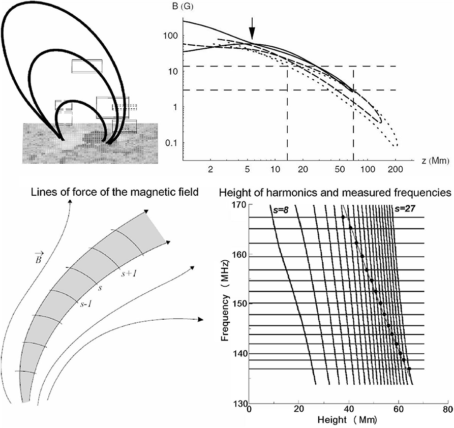
Figure 12. (Top, left) Position of fiber bursts within the associated loops. (Top, right) The magnetic field as a function of height for various fiber loops; thin dashed lines show the limits of the region where the bursts were observed. From Aurass et al. (2005), reproduced with permission © ESO. (Bottom) Zebra pattern formation due to the double plasma resonance effect. Left: Structure of the source with the harmonic levels marked. Right: Height of the gyrofrequency harmonic levels as a function of frequency; the horizontal lines represent the measured peak frequencies. The points mark the intersections that are consistent with hydrostatic variation of the electron density with height. Adapted from Zlotnik (2009).

In a recent work, Bouratzis et al. (2019) deduced an average magnetic field of 4.6 G with a dispersion of 1.5 G, from the analysis of a large number of fiber bursts observed with the ARTEMIS/JLS radiospectrograph between 250 and 470 MHz, assuming whistler origin for the fibers and a hydrostatic coronal model at $T_e=2\times 10^6$ K and a base density 4× that of the Newkirk density model. They obtained similar results from the analysis of the tracks on the dynamic spectrum of 38 fiber groups, without assuming any specific density model. Observing at higher frequencies (1–2 GHz) with the VLA, Wang et al. (2017) reported 62 G at 10 Mm and 8 G at 36 Mm.

Let us now consider zebra patterns, which also originate in post-flare loops and for which three principal mechanisms have been proposed (see Zlotnik, 2009 for a review, also Chernov, 2011). In one of them, they are attributed to the coalescence of electrostatic Bernstein waves at the harmonics of the electron gyrofrequency, ω = sω_ce, and plasma waves at the upper hybrid frequency, ${\omega }_{UH}=\sqrt{{\omega }_p^2+{\omega }_{ce}^2}\simeq {\omega }_p$ for ω_ce ≪ ω_p. The resulting frequency is ω = ω_p + sω_ce. The separation of spectral maxima should then be equal to the electron gyrofrequency and this gives directly the magnetic field. Note also that in this model all stripes are produced in the same region, which must be homogeneous; the wavy form of the pattern is attributed to magnetic field variations with time.

As an example of the field values deduced from this model, the frequency separation of the zebra stripes in Figure 11, ranging from 5 to 10 MHz, would imply values of 1.8–3.6 G; note, however that the frequency separation at a given time is not constant, as it should be if the stripes were at the harmonics of the gyrofrequency. The low field values that often arise from the Bernstein waves interpretation of zebras is considered as an argument against its validity (Zlotnik, 2009), another one being its inability to account for more than ~ 10 stripes.

One alternative, widely accepted interpretation, attributes the zebra pattern to the double plasma resonance (see Zheleznyakov and Zlotnik, 1975; Zheleznyakov et al., 2016), in which the emission occurs at locations where the upper hybrid frequency is equal to a harmonic of the gyrofrequency. In this case different stripes are produced in different regions (Figure 12, bottom row) and the frequency separation of the stripes is (Zlotnik, 2009):

$\begin{array}{ll}\frac{\Delta \omega }{{\omega }_{ce}}=\frac{L_B}{|L_N-L_B|}\simeq \frac{L_B}{L_N}& (40)\end{array}$

where L_N and L_B are the density and magnetic field scales respectively; thus Δω can be significantly smaller than the gyrofrequency. Another important point is that the growth rate is ~100 times greater than in the case of Bernstein modes.

In order to extract physical information on the basis of the double plasma resonance process, one has to model both the magnetic field and the density. Zlotnik et al. (2003) used extrapolations of the photospheric magnetic field together with a hydrostatic density variation to fit the observed frequency of the stripes. They deduced harmonic numbers in the range of s = 13 at 173 MHz to s = 27 at 143 MHz (their Figure 5), which correspond to field strengths of 4.9–1.9 G respectively; these are higher by a factor of 2–4 than the values that would be derived from the Bersnstein wave model and the frequency separation of the stripes of 3.3–2.5 MHz, deduced from their Figure 5 (1.2–0.9 G). However, the temperatures associated with their hydrostatic model were rather low, only 0.8–1.18 × 10⁶ K.

Further observational evidence in favor of the double plasma resonance has been provided by Chen et al. (2011) for an event observed with the VLA in the 1.2–1.4 MHz range, who found that zebra stripes were at different locations; using the method of Zlotnik et al. (2003), they deduced s = 8–13 and B = 62 to 35 G at estimated heights of 57–75 Mm, together with L_N ≃ 140 Mm and L_N/L_B ≃ 4.4. A similar conclusion about the emission mechanism was reached by Altyntsev et al. (2011), from the analysis of 6 events in the microwave range, while Altyntsev et al. (2005) favored the Bernstein wave model for one microwave event. Using the UTR-2 radio telescope in the decametric frequency range (16.5–33 MHz), Stanislavsky et al. (2015) obtained a field value of 0.43 G under the Bernstein mode assumption. At the other end of the radio spectrum (1.4 GHz), Karlický and Yasnov (2018) measured 0.84–37.31 G corresponding to electron densities of 0.026 × 10¹⁰ to 16.03 × 10¹⁰ cm⁻³.

A third model attributes zebra patterns to whistler waves (for details see Chernov, 2006, 2011); in this case a magnetic trap is filled with periodic whistler emission zones separated by their absorption zones. Yasnov and Chernov (2020) noted that this model gave a reasonable magnetic field of 4.5 G, whereas the double plasma resonance model gave only 1–1.5 G together with plasma β > 1, for an event at 183 MHz that they analyzed.

8. Type II Bursts

Type II bursts are due to coherent emission at the plasma frequency and/or its harmonic, excited by shock waves propagating up in the corona with a super-Alfvénic speed (Vršnak and Cliver, 2008). As type II bursts often extend into interplanetary space, they provide a magnetic field diagnostic over a very extended distance range. If the Alfvén Mach number M_A = υ/υ_A could be estimated, the Alfvén speed that contains information about the magnetic field would be deduced from the frequency drift and the density scale.

For emission at the fundamental, under hydrostatic equilibrium with a density scale, L_N, along the shock trajectory, the velocity of the exciter is related to the frequency drift rate, df/dt, through:

$\begin{array}{ll}\upsilon =\frac{2\sqrt{\pi m_e}}{e\sqrt{N_e}}{L}_N\frac{df}{dt}& (41)\end{array}$

which, combined with the definition of the Alfvén speed (38) gives:

$\begin{array}{ll}B=4\pi \frac{\sqrt{m_e{m}_p}}{e}\frac{L_N}{M_A}\frac{df}{dt}& (42)\end{array}$

B is a factor of 2 smaller if the emission is at the harmonic. It is obvious that an estimate of L_N along the shock trajectory (which is not necessarily in the vertical direction), is required. Moreover, a density-height model is needed to associate the magnetic field to a particular height in the corona. Thus, if no additional information is available from other observations, the measurement of the magnetic field using (42) is highly model dependent.

Several decades ago, Takakura (1964) assumed M_A = 1 to get estimates of the magnetic field; this is not too bad an assumption since type II shocks are weak, with Mach numbers not too far from unity. The possibility of a more accurate estimate of M_A from the band splitting of certain type II's (Figure 13, top) was first proposed by Smerd et al. (1974). Band splitting is interpreted in terms of the density jump at the shock front, i.e., between the uncompressed plasma in front of the shock and the compressed plasma behind it. The Alfvén Mach number, M_A, is related to the compression, X, of the shock through the Rankine-Hugoniot relation which, under the quasi-perpendicular shock approximation and for plasma β << 1, can be written as (Vršnak et al., 2002):

$\begin{array}{ll}{M}_A=\sqrt{\frac{X(X+5)}{2(4-X)}}& (43)\end{array}$

The compression, X, is defined as:

$\begin{array}{ll}X=\frac{N_{e2}}{N_{e1}}={\left(\frac{f_2}{f_1}\right)}^2={\left(\frac{f_2-f_1}{f_1}+1\right)}^2& (44)\end{array}$

here N_e2 and N_e1 are the electron densities behind and in front of the shock and f₂ and f₁ the frequencies of the corresponding bands of type II emission.

FIGURE 13

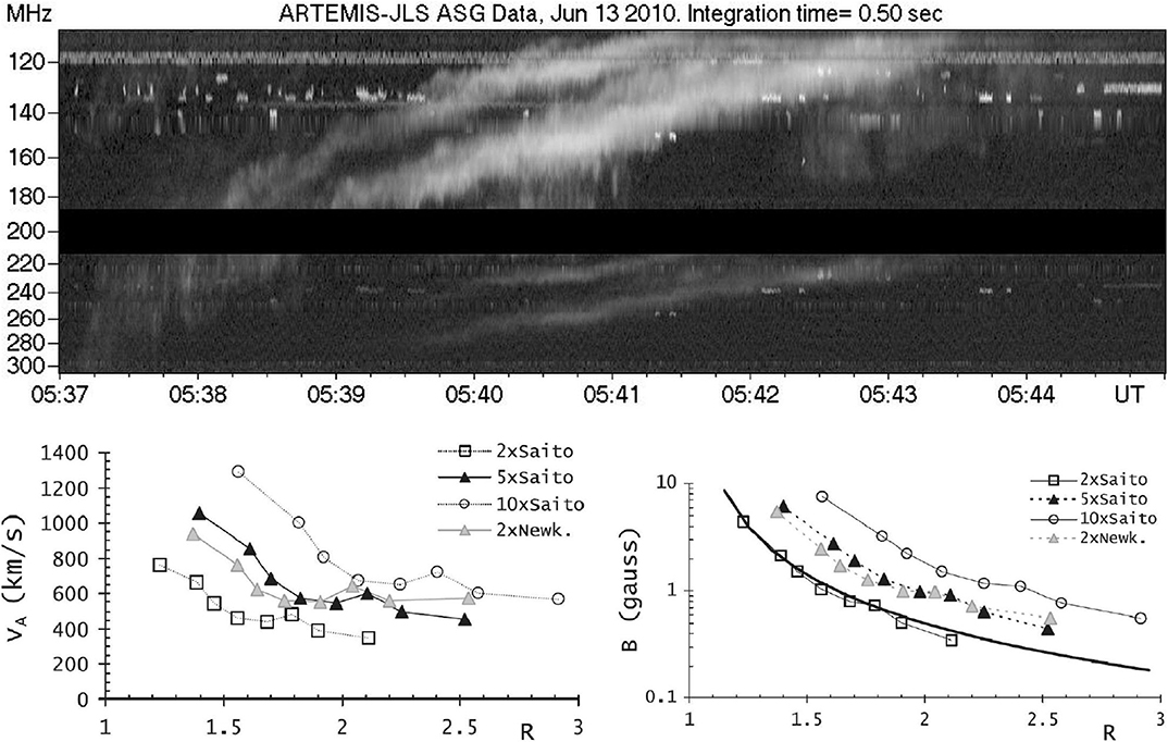
Figure 13. (Top) A Type II burst with band split and fundamental/harmonic structure observed with ARTEMIS/JLS; data selected by S. Armatas. (Bottom) Alfvén speed (left) and magnetic field (right) as a function of radial distance in R_⊙, computed from type II band splitting by Vršnak et al. (2002), for various coronal density models. The thick line in the right panel shows the empirical relation of Dulk and McLean (1978); reproduced with permission © ESO.

On the basis of band splitting, Smerd et al. (1974) deduced Mach numbers between 1.2 and 1.5. In an extensive work, Vršnak et al. (2002) investigated 18 low frequency events; their measurements of M_A group around 1.4 and their results on the average Alfvén speed and magnetic field are shown in the bottom panels of Figure 13 for various coronal density models. In a subsequent work, Vršnak et al. (2004) extended their investigation to events in the km wavelength range, which occur in the interplanetary space out to the Earth and proposed the empirical relation B∝R⁻², while Mahrous et al. (2018) reported ~4 G at heliocentric R ~ 2.6 R_⊙ to ~0.62 G at R ~ 3.77 R_⊙.

Other works have employed additional information, together with the band splitting, to reduce model dependent uncertainties. For example, Cho et al. (2007) used MK4 coronameter data to constrain the electron density and deduced magnetic field of 1.3–0.4 G at heights of 1.6–2.1 R_⊙. Similarly, Kumari et al. (2017) and Kumari et al. (2019) derived the electron density from white light space born coronograph images and reported 0.47–0.44 G at heliocentric 2.61–2.74 R_⊙ and 1.21–0.5 G at heliocentric 1.58–2.15 R_⊙, respectively. Gopalswamy et al. (2012), using additional information on the geometry of the shock from SDO/AIA images, determined the coronal magnetic field to be in the range of 1.3–1.5 G at heliocentric 1.2–1.5 R_⊙. Finally, we mention the work of Mancuso et al. (2019), who analyzed metric spectral and imaging observations, together with EUV images of a shock-streamer interaction and concluded that the magnetic field varied as B(R) = (12.6±2.5)R⁻⁴ in the heliocentric distance range of 1.11–2.0 R_⊙; this gives 8.6 and 0.78 G at the limits of the above range of R.

9. Discussion and Conclusions

All things considered, radio observations offer the most reliable quantitative estimates of the magnetic field in the solar TR and the corona. However, there are three aspects that one should bear in mind: (a) That the magnetic field is often measured not over a 2-D field of view as in the photosphere but at particular locations, (b) that the vast majority of the measurements refers to active regions or bursts and not to the quiet Sun, and (c) that some methods require additional information for the computation of the magnetic field, such as the density scale and the height of the emission; this has to be provided by other observations, by models, or even by estimates.

The polarization of f-f emission at short radio λ can provide magnetic field maps over a two-dimensional field of view, which are closest to the concept of photospheric Zeeman magnetograms. Its principal limitation is the instrumental sensitivity to low circular polarization, consequently at present the magnetic field can be measured in plages but not yet in the quiet Sun. As in the case of photospheric magnetograms, the measurements reflect the value of the field over the entire region of formation of radiation which can be quite extended in height, at longer wavelengths in particular. Information about the height variation of the field can be provided by observations at different wavelengths. At longer, metric wavelengths, the situation is more complicated, both due to the difficulties in polarization measurements and the refracted and scattered ray-path geometry of the emission.

Gyro-resonance emission at relatively low heights ≤ 0.1R_⊙ above sunspots provides directly the magnetic field as a function of temperature, rather than the height, except at the limb where high-resolution imaging can provide direct height measurements. The height variation can be probed by combining radio spectral measurements and magnetic field extrapolations, and efforts are underway to use the radio measurements as constraints to improve such extrapolations (Fleishman et al., 2019). Cyclotron lines can provide important information, but so far only a few cases have been reported. Gyrosyncrotron emission from microwave bursts has long been difficult to use due to its complex dependence on many physical parameters, but recently the method has come into its own with the advent of microwave imaging spectroscopy, both in the case of radio CMEs and in fitting of spatially resolved spectra in the flaring region. Other papers in this special research topic collection are dedicated to covering this new method.

Higher in the corona, from 0.05 to 0.4 R_⊙ above the photosphere, the inversion of circular polarization due to propagation effects is a powerful tool for measuring the active region magnetic field. A very important advantage of this method is that it is independent of the emission mechanism. At the same time, the theory of wave propagation gives us a warning not to take at face value the observed circular polarization, as it does not always reflect the properties of its source. The general picture that emerges from these studies is that the magnetic field drops from about 100 G to about 5 Gauss in this height range.

Bursts at metric wavelengths can be used for estimates of the magnetic field in a height range that overlaps that of polarization inversion methods and extends into the interplanetary space. Methods based on fiber bursts, zebra patterns and the band splitting of type II bursts have been discussed in this review. Generated by coherent radiation processes, these emissions are more difficult to model than those that are due to incoherent processes and this has a bearing on their use for magnetic field measurements. Moreover, the results have a high dependency on models of the coronal density.

Going to heliocentric distances of 5 R_⊙ and beyond, Faraday rotation of celestial sources or of signals from interplanetary space probes has been employed to diagnose the magnetic field in structures such as CMEs, which is very important information in the context of space weather. The main difficulty here is the untangling of the magnetic field from the electron density, since both contribute to the rotation of the plane of polarization.

Several years ago, Dulk and McLean (1978) combined all radio data available at the time and explored the variation of the magnetic field with height. They derived the following empirical relation, for the range 1.02 ≤ R/R_⊙ ≤ 10, where R is the heliocentric distance:

$\begin{array}{ll}B=0.5{(R/R_{\odot }-1)}^{-1.5}\text{ G}& (45)\end{array}$

which fitted the data to about a factor of three. Subsequently, Gopalswamy et al. (1986) assuming that type I bursts are produced by shocks, suggested the following relation, valid for 1.09 ≤ R/R_⊙ ≤ 1.73:

$\begin{array}{ll}B=0.41{(R/R_{\odot }-1)}^{-0.89}\text{ G}& (46)\end{array}$

Although it is obviously impossible to describe the complex coronal magnetic field with simple expressions such as the above, it is still instructive to compare them with the more recent observational results. A plot of magnetic field intensity as a function of height from the photosphere, using measurements compiled in this review, is shown in Figure 14. Different symbols denote different methods, as explained in the figure and discussed below; we have not included values at low heights from f-f or g-r emission. The thick straight line shows the Dulk-McLean relation; although this relation does not coincide with the linear regression line for this data set, we note that there are points on either side of the line.

FIGURE 14

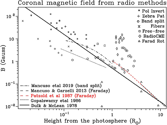
Figure 14. The coronal magnetic field as a function of height, up to 12 R_⊙, measured by radio methods, indicated by different symbols. The empirical relations of Mancuso et al. (2019) and Mancuso and Garzelli (2013), Pätzold et al. (1987), Gopalswamy et al. (1986) are plotted as dashed-dotted, dashed, red dashed and dotted lines respectively. The full straight line is the empirical relation of Dulk and McLean (1978).

The data plotted in Figure 14 are by no means exhaustive, still they are indicative. Although the decline of the field intensity with height is clear, there is a lot of scatter, sometimes more than a factor of ten at the same height. The set of measurements based on polarization reversal (* in the plot), although made by different authors and for different active regions, is the most self-consistent set and appears robust. This is not surprising, as the associated processes are well understood and the polarization measurements quite reliable. The free-free measurements of Ramesh et al. (2010) at metric λ (open squares) appear consistent with the polarization inversion measurements.

Most of the scatter in Figure 14 is due to measurements based on metric bursts, which emit through coherent mechanisms. The majority of the results from zebra patterns and fiber bursts (x and + in the plot), with the exception of those of Chen et al. (2011), are well below the Dulk-McLean curve; these are better fitted by the Gopalswamy et al. (1986) model which, however, is below most other measurements. As for type II split-band results (open circles and dash-dot line), we note that most fall near the Dulk-McLean relation, except for the measurements of Mahrous et al. (2018) in the height range 2-3 R_⊙, which are well above. Some radio CME results (diamonds in the figure) are close to the Dulk-McLean curve, while others, in particular those of Mondal et al. (2020), are well above. Finally, the majority of results from Faraday rotation (triangles and the dashed line) fall quite close to the Dulk-McLean line, with the exception of the MESSENGER results of Wexler et al. (2019), which are too low.

In order to explain these differences, one should consider: (a) that physical conditions can be very different above active regions, in bursts and in CMEs and certainly quite different from the quiet Sun, (b) the variety of physical mechanisms that have been proposed for the same type of incoherent emission, (c) that the height ascribed to the measured magnetic field is often computed on the basis of a coronal density model, which may not be applicable to the actual situation; the height problem is also illustrated by the fact that many authors just quote field intensities without specifying the height, and (d) the measurements were carried out at different phases and cycles of solar activity.

What can we hope for the future? The answer is rather trivial: better observations and improved theory will provide more accurate measurements of the coronal magnetic field. Higher spatial resolution and better sensitivity to circular polarization are indispensable for measuring the magnetic field in the chromospheric network, while wide spectral coverage is necessary to follow its evolution till the network fades in the low corona. With sufficient spatial resolution and high sensitivity in V we might even be able to measure the magnetic field in coronal holes and coronal loops at metric wavelengths. High spectral resolution is required for the detection of cyclotron lines, for polarization inversion and, together with narrow band receivers, for linear polarization due to propagation effects. Last but not least, as the perihelion of the Parker Solar Probe comes closer to the Sun, we will have in situ measurements in the outer solar corona (~ 10 R_⊙); results from the first perihelion passage (100 to 36 R_⊙) have shown a 1/r² dependence of the background magnetic field, with an intensity of ~80 nT near perihelion (Bale et al., 2019).

Better 2D imaging together with high spectral resolution will provide us with the observational base for a better understanding of microwave, decimetric and metric burst fine structure, and will help us obtain better information on active regions in the TR and low corona. The Low Frequency Array (LOFAR), as well as the VLA, EOVSA, and the Murchison Widefield Array (MWA) have already opened an exciting new era of imaging spectroscopy. Among the new instruments, the Siberian Solar Radioheliograph (SSRH) is starting, a new, solar-dedicated system for the Owens Valley Radio Observatory-Long Wavelength Array (OVRO-LWA) is nearing completion, the Chinese Mingantu Ultrawide Spectral Radioheliograph (MUSER) is in operation, the next generation VLA (ngVLA) is under consideration, while the Square Kilometer Array (SKA) is not too far below the horizon. The Atacama Large mm and sub-mm Array (ALMA) cannot observe solar circular polarization yet (see Loukitcheva, 2020 in this special research topic collection); when this option becomes available, a 2,000 G sunspot will give an easily measurable polarization of 10% at 3 mm (Equation 23). In addition, the continued operation of existing instruments, such as the Nançay radioheliograph and RATAN-600 must be assured; the shut down of the Nobeyama radioheliograph on March 31, 2020 was a severe loss to the community.

In the field of theory, modeling has already given impressive results for sunspot associated emission and microwave bursts, but there is always room for more, particularly for bursts. With incoherent mechanisms giving low estimates of the magnetic field, a better understanding of the emission and improved modeling is highly desirable.

Author Contributions

Both authors reviewed the literature, selected the material presented in this review, and have approved it for publication.

Funding

This work was supported in part by NSF grant AST-1910354 to the New Jersey Institute of Technology.

Conflict of Interest

The authors declare that the research was conducted in the absence of any commercial or financial relationships that could be construed as a potential conflict of interest.

Acknowledgments

In preparing this review the authors used publicly available data from a number of instruments: the Nobeyama Radioheliograph (NoRH), the Siberian Solar Radio Telescope (SSRT), the RATAN-600 radio telescope, the Michelson Doppler Imager aboard the Solar and Heliospheric Observatory (SOHO) and the Helioseismic and Magnetic Imager (HMI) aboard the Solar Dynamics Observatory (SDO); dynamic spectra were provided by the ARTEMIS/JLS radio spectrograph group. We are grateful to all those that operate these instruments and make their data available to the community. Comments by Dr. L. Klein of Meudon observatory on an early version of the manuscript are gratefully acknowledged.

References

Akhmedov, S. B., Gelfreikh, G. B., Bogod, V. M., and Korzhavin, A. N. (1982). The measurement of magnetic fields in the solar atmosphere above sunspots using gyro-resonance emission. Solar Phys. 79, 41–58. doi: 10.1007/BF00146972

CrossRef Full Text | Google Scholar

Alissandrakis, C. E. (1999). “Magnetic field diagnostics in the low corona from microwave circular polarization inversion,” in Proceedings of the Nobeyama Symposium, eds T. S. Bastian, N. Gopalswamy, and K. Shibasaki, 53–58.

Google Scholar

Alissandrakis, C. E. (2020). Structure of the solar atmosphere: a radio perspective. Front. Astron. Space Sci. 7:574460. doi: 10.3389/fspas.2020.574460

CrossRef Full Text | Google Scholar

Alissandrakis, C. E., Bogod, V. M., Kaltman, T. I., Patsourakos, S., and Peterova, N. G. (2019a). Modeling of the sunspot-associated microwave emission using a new method of dem inversion. Solar Phys. 294:23. doi: 10.1007/s11207-019-1406-x

CrossRef Full Text | Google Scholar

Alissandrakis, C. E., Borgioli, F., Chiuderi Drago, F., Hagyard, M., and Shibasaki, K. (1996). Coronal magnetic fields from microwave polarization observations. Solar Phys. 167, 167–179. doi: 10.1007/BF00146335

CrossRef Full Text | Google Scholar

Alissandrakis, C. E., Bouratzis, C., and Hillaris, A. (2019b). High-resolution observations with artemis-jls and the NRH. III. Spectroscopy and imaging of fiber bursts. Astron. Astrophys. 627:A133. doi: 10.1051/0004-6361/201935627

CrossRef Full Text | Google Scholar

Alissandrakis, C. E., and Chiuderi-Drago, F. (1994). Detection of linear polarization in the microwave emission of solar active regions. Astrophys. J. 428:L73. doi: 10.1086/187396

CrossRef Full Text | Google Scholar

Alissandrakis, C. E., and Kundu, M. R. (1984). Center-to-limb variation of a sunspot-associated microwave source. Astron. Astrophys. 139, 271–284.

Google Scholar

Alissandrakis, C. E., Kundu, M. R., and Lantos, P. (1980). A model for sunspot associated emission at 6 CM wavelength. Astron. Astrophys. 82, 30–40.

Google Scholar

Alissandrakis, C. E., Lantos, P., and Nicolaidis, E. (1985). Coronal structures observed at metric wavelengths with the Nançay radioheliograph. Solar Phys. 97, 267–282. doi: 10.1007/BF00165990

CrossRef Full Text | Google Scholar

Alissandrakis, C. E., Nindos, A., and Kundu, M. R. (1993). Evidence for ordinary mode emission from microwave bursts. Solar Phys. 147, 343–358. doi: 10.1007/BF00690724

CrossRef Full Text | Google Scholar

Alissandrakis, C. E., and Preka-Papadema, P. (1984). Microwave emission and polarization of a flaring loop. Astron. Astrophys. 139, 507–511.

Google Scholar

Altyntsev, A. T., Kuznetsov, A. A., Meshalkina, N. S., Rudenko, G. V., and Yan, Y. (2005). On the origin of microwave zebra pattern. Astron. Astrophys. 431, 1037–1046. doi: 10.1051/0004-6361:20048337

CrossRef Full Text | Google Scholar

Altyntsev, A. T., Lesovoi, S. V., Meshalkina, N. S., Sych, R. A., and Yan, Y. (2011). Radioheliograph observations of microwave bursts with zebra structures. Solar Phys. 273, 163–177. doi: 10.1007/s11207-011-9856-9

CrossRef Full Text | Google Scholar

Anfinogentov, S. A., Stupishin, A. G., Mysh'yakov, I. I., and Fleishman, G. D. (2019). Record-breaking coronal magnetic field in solar active region 12673. Astrophys. J. 880:L29. doi: 10.3847/2041-8213/ab3042

CrossRef Full Text | Google Scholar

Aurass, H., Rausche, G., Mann, G., and Hofmann, A. (2005). Fiber bursts as 3D coronal magnetic field probe in postflare loops. Astron. Astrophys. 435, 1137–1148. doi: 10.1051/0004-6361:20042199

CrossRef Full Text | Google Scholar

Bain, H. M., Krucker, S., Saint-Hilaire, P., and Raftery, C. L. (2014). Radio imaging of a type IVM radio burst on the 14th of august 2010. Astrophys. J. 782:43. doi: 10.1088/0004-637X/782/1/43

CrossRef Full Text | Google Scholar

Bale, S. D., Badman, S. T., Bonnell, J. W., Bowen, T. A., Burgess, D., Case, A. W., et al. (2019). Highly structured slow solar wind emerging from an equatorial coronal hole. Nature 576, 237–242. doi: 10.1038/s41586-019-1818-7

PubMed Abstract | CrossRef Full Text | Google Scholar

Bandiera, R. (1982). Diagnostic of coronal magnetic fields from microwave polarization reversal. Astron. Astrophys. 112, 52–60.

Google Scholar

Bastian, T. S. (1995). Angular scattering of radio waves: Implications for mode coupling in the solar corona. Astrophys. J. 439:494. doi: 10.1086/175190

CrossRef Full Text | Google Scholar

Bastian, T. S., Benz, A. O., and Gary, D. E. (1998). Radio emission from solar flares. Annu. Rev. Astron. Astrophys. 36, 131–188. doi: 10.1146/annurev.astro.36.1.131

CrossRef Full Text | Google Scholar

Bastian, T. S., Dulk, G. A., and Leblanc, Y. (1996). High-resolution microwave observations of the quiet solar chromosphere. Astrophys. J. 473:539. doi: 10.1086/178165

CrossRef Full Text | Google Scholar

Bastian, T. S., Pick, M., Kerdraon, A., Maia, D., and Vourlidas, A. (2001). The coronal mass ejection of 1998 April 20: direct imaging at radio wavelengths. Astrophys. J. Lett. 558, L65–L69. doi: 10.1086/323421

CrossRef Full Text | Google Scholar

Benz A. O. and Mann, G. (1998). Intermediate drift bursts and the coronal magnetic field. Astron. Astrophys. 333, 1034–1042.

Google Scholar

Bird, M. K. (2007). Coronal Faraday rotation of occulted radio signals. Astron. Astrophys. Trans. 26, 441–453. doi: 10.1080/10556790701595236

CrossRef Full Text | Google Scholar

Bogod, V. M., Alissandrakis, C. E., Kaltman, T. I., and Tokhchukova, S. K. (2015). Ratan-600 observations of small-scale structures with high spectral resolution. Solar Phys. 290, 7–20. doi: 10.1007/s11207-014-0526-6

CrossRef Full Text | Google Scholar

Bogod, V. M., Garaimov, V. I., Zheleznyakov, V. V., and Zlotnik, E. Y. (2000). Detection of a cyclotron line in the radio spectrum of a solar active region and its interpretation. Astron. Rep. 44, 271–277. doi: 10.1134/1.163850

CrossRef Full Text | Google Scholar

Bogod, V. M., and Gelfreikh, G. B. (1980). Measurements of the magnetic field and the gradient of temperature in the solar atmosphere above a flocculus using radio observations. Solar Phys. 67, 29–46. doi: 10.1007/BF00146680

CrossRef Full Text | Google Scholar

Bogod, V. M., Gelfreikh, G. B., Ryabov, B. I., and Hafizov, S. R. (1993). “Coronal magnetic fields from the effect of the double inversion of circular polarization of radio emission,” in Astronomical Society of the Pacific Conference Series (San Francisco, CA), Vol. 46, 302. doi: 10.1017/S0252921100029298

CrossRef Full Text | Google Scholar

Bogod, V. M., Stupishin, A. G., and Yasnov, L. V. (2012). On magnetic fields of active regions at coronal heights. Solar Phys. 276, 61–73. doi: 10.1007/s11207-011-9850-2

CrossRef Full Text | Google Scholar

Borovik, V. N., Medar', V. G., and Korzhavin, A. N. (1999). First measurements of the magnetic field in a coronal hole from RATAN-600 radio observations of the Sun. Astron. Lett. 25, 250–257.

Google Scholar

Bouratzis, C., Hillaris, A., Alissandrakis, C. E., Preka-Papadema, P., Moussas, X., Caroubalos, C., et al. (2019). High resolution observations with artemis-jls. ii. type iv associated intermediate drift bursts. Astron. Astrophys. 625:A58. doi: 10.1051/0004-6361/201834792

CrossRef Full Text | Google Scholar

Brosius, J. W., and White, S. M. (2006). Radio measurements of the height of strong coronal magnetic fields above sunspots at the solar limb. Astrophys. J. Lett. 641, L69–L72. doi: 10.1086/503774

CrossRef Full Text | Google Scholar

Cargill, P. J. (2009). Coronal magnetism: difficulties and prospects. Space Sci. Rev. 144, 413–421. doi: 10.1007/s11214-008-9446-9

CrossRef Full Text | Google Scholar

Carley, E. P., Vilmer, N., Simoes, P. J. A., and Ó Fearraigh, B. (2017). Estimation of a coronal mass ejection magnetic field strength using radio observations of gyrosynchrotron radiation. Astron. Astrophys. 608:A137. doi: 10.1051/0004-6361/201731368

CrossRef Full Text | Google Scholar

Chambe, G., and Lantos, P. (1971). Influence of helium and heavy elements on the radio absorption coefficient. Solar Phys. 17, 97–98. doi: 10.1007/BF00152864

CrossRef Full Text | Google Scholar

Chen, B., Bastian, T. S., Gary, D. E., and Jing, J. (2011). Spatially and spectrally resolved observations of a zebra pattern in a solar decimetric radio burst. Astrophys. J. 736:64. doi: 10.1088/0004-637X/736/1/64

CrossRef Full Text | Google Scholar

Chen, B., Shen, C., Gary, D. E., Reeves, K. K., Fleishman, G. D., Yu, S., et al. (2020). Measurement of magnetic field and relativistic electrons along a solar flare current sheet. arXiv:2005.12757. doi: 10.1038/s41550-020-1147-7

CrossRef Full Text | Google Scholar

Chernov, G. (2011). Fine Structure of Solar Radio Bursts Berlin: Springer. doi: 10.1007/978-3-642-20015-1

CrossRef Full Text | Google Scholar

Chernov, G. P. (2006). Solar radio bursts with drifting stripes in emission and absorption. Space Sci. Rev. 127, 195–326. doi: 10.1007/s11214-006-9141-7

CrossRef Full Text | Google Scholar

Chiuderi Drago, F., Alissandrakis, C., and Hagyard, M. (1987). Microwave emission above steady and moving sunspots. Solar Phys. 112, 89–105. doi: 10.1007/BF00148490

CrossRef Full Text | Google Scholar

Cho, K. S., Lee, J., Gary, D. E., Moon, Y. J., and Park, Y. D. (2007). Magnetic field strength in the solar corona from type ii band splitting. Astrophys. J. 665, 799–804. doi: 10.1086/519160

CrossRef Full Text | Google Scholar

Cohen, M. H. (1960). Magnetoionic mode coupling at high frequencies. Astrophys. J. 131:664. doi: 10.1086/146878

CrossRef Full Text | Google Scholar

Dulk, G. A., and McLean, D. J. (1978). Coronal magnetic fields. Solar Phys. 57, 279–295. doi: 10.1007/BF00160102

CrossRef Full Text | Google Scholar

Efimov, A. I., Lukanina, L. A., Rogashkova, A. I., Samoznaev, L. N., Chashei, I. V., Bird, M. K., et al. (2015). Coronal radio occultation experiments with the helios solar probes: correlation/spectral analysis of faraday rotation fluctuations. Solar Phys. 290, 2397–2408. doi: 10.1007/s11207-015-0687-y

CrossRef Full Text | Google Scholar

Fleishman, G., Mysh'yakov, I., Stupishin, A., Loukitcheva, M., and Anfinogentov, S. (2019). Force-free field reconstructions enhanced by chromospheric magnetic field data. Astrophys. J. 870:101. doi: 10.3847/1538-4357/aaf384

CrossRef Full Text | Google Scholar

Fleishman, G. D., Gary, D. E., Chen, B., Kuroda, N., Yu, S., and Nita, G. M. (2020). Decay of the coronal magnetic field can release sufficient energy to power a solar flare. Science 367, 278–280. doi: 10.1126/science.aax6874

PubMed Abstract | CrossRef Full Text | Google Scholar

Fleishman, G. D., and Melnikov, V. F. (2003). Gyrosynchrotron emission from anisotropic electron distributions. Astrophys. J. 587, 823–835. doi: 10.1086/368252

CrossRef Full Text | Google Scholar

Gary, D. E., Chen, B., Dennis, B. R., Fleishman, G. D., Hurford, G. J., Krucker, S., et al. (2018). Microwave and hard x-ray observations of the 2017 September 10 solar limb flare. Astrophys. J. 863:83. doi: 10.3847/1538-4357/aad0ef

CrossRef Full Text | Google Scholar

Gelfreikh, G. (2004) “Coronal magnetic field measurements through bremsstrahlung emission,” in Solar and Space Weather Radiophysics. Astrophysics and Space Science Library, Vol. 314 (Dordrecht: Springer). 10.1007/1-4020-2814-8_6.

Google Scholar

Gelfreikh, G. B. (1998). “Three-dimensional structure of the magnetospheres of solar active regions from radio observations (invited review),” in Three-Dimensional Structure of Solar Active Regions, Vol. 155, eds C. E. Alissandrakis and B. Schmieder, Astronomical Society of the Pacific Conference Series (San Francisco, CA), 110.

Google Scholar

Gelfreikh, G. B., Peterova, N. G., and Riabov, B. I. (1987). Measurements of magnetic fields in solar corona as based on the radio observations of the inversion of polarization of local sources at microwaves. Solar Phys. 108, 89–97. doi: 10.1007/BF00152079

CrossRef Full Text | Google Scholar

Gelfreikh, G. B., Pilyeva, N. A., and Ryabov, B. I. (1997). On the gradient of coronal magnetic fields from radio observations. Solar Phys. 170, 253–264. doi: 10.1023/A:1004967202294

CrossRef Full Text | Google Scholar

Gopalswamy, N., and Kundu, M. R. (1987). Simultaneous radio and white light observations of the 1984 June 27 coronal mass ejection event. Solar Phys. 114, 347–362. doi: 10.1007/BF00167350

CrossRef Full Text | Google Scholar

Gopalswamy, N., Nitta, N., Akiyama, S., Mäkelä, P., and Yashiro, S. (2012). Coronal magnetic field measurement from EUV images made by the solar dynamics observatory. Astrophys. J. 744:72. doi: 10.1088/0004-637X/744/1/72

CrossRef Full Text | Google Scholar

Gopalswamy, N., Thejappa, G., Sastry, C. V., and Tlamicha, A. (1986). Estimation of coronal magnetic fields using type-i emission. Bull. Astron. Instit. Czechoslov. 37:115.

Google Scholar

Gopalswamy, N., White, S. M., and Kundu, M. R. (1991). Large-scale features of the sun at 20 centimeter wavelength. Astrophys. J. 379:366. doi: 10.1086/170512

CrossRef Full Text | Google Scholar

Gopalswamy, N., Zheleznyakov, V. V., White, S. M., and Kundu, M. R. (1994). Polarization features of solar radio emission and possible existence of current sheets in active regions. Solar Phys. 155, 339–350. doi: 10.1007/BF00680599

CrossRef Full Text | Google Scholar

Grebinskij, A., Bogod, V., Gelfreikh, G., Urpo, S., Pohjolainen, S., and Shibasaki, K. (2000). Microwave tomography of solar magnetic fields. Astron. Astroph. Suppl. Ser. 144, 169–180. doi: 10.1051/aas:2000202

CrossRef Full Text | Google Scholar

Hagyard, M. J., Teuber, D., West, E. A., Tand berg-Hanssen, E., Henze, W. J., Beckers, J. M., et al. (1983). Vertical gradients of sunspot magnetic fields. Solar Phys. 84, 13–31. doi: 10.1007/BF00157439

CrossRef Full Text | Google Scholar

Henze, W. J, Tandberg-Hanssen, E., Hagyard, M. J., West, E. A., Woodgate, B. E., Shine, R. A., et al. (1982). Observations of the longitudinal magnetic field in the transition region and photosphere of a sunspot. Solar Phys. 81, 231–244. doi: 10.1007/BF00151299

CrossRef Full Text | Google Scholar

Ingleby, L. D., Spangler, S. R., and Whiting, C. A. (2007). Probing the large-scale plasma structure of the solar corona with faraday rotation measurements. Astrophys. J. 668, 520–532. doi: 10.1086/521140

CrossRef Full Text | Google Scholar

Kakinuma, T., and Swarup, G. (1962). A model for the sources of the slowly varying component of microwave solar radiation. Astrophys. J. 136:975. doi: 10.1086/147450

CrossRef Full Text | Google Scholar

Kaltman, T. I., and Bogod, V. M. (2019) On detecting the fourth gyrofrequency harmonic in microwave emission spectra above sunspots. Cosmic Res. 57, 1-9. 10.1134/S0010952519010040

Kaltman, T. I., Korzhavin, A. N., and Peterova, N. G. (2007). The self-inversion of the sign of circular polarization in “Halo” microwave sources. Solar Phys. 242, 125–142. doi: 10.1007/s11207-007-0057-5

CrossRef Full Text | Google Scholar

Karlický, M., and Yasnov, L. V. (2018). Determination of plasma parameters in radio sources of solar zebra-patterns based on relations between the zebra-stripe frequencies and gyro-harmonic numbers. Astrophys. J. 867:28. doi: 10.3847/1538-4357/aae1f8

CrossRef Full Text | Google Scholar

Klein, K. L., and Trottet, G. (1984). Gyrosynchrotron radiation from a source with spatially varying field and density. Astron. Astrophys. 141, 67–76.

Google Scholar

Kontogeorgos, A., Tsitsipis, P., Caroubalos, C., Moussas, X., Preka-Papadema, P., Hilaris, A., et al. (2006). The improved Artemis iv multichannel solar radio spectrograph of the University of Athens. Exp. Astron. 21, 41–55. doi: 10.1007/s10686-006-9066-x

CrossRef Full Text | Google Scholar

Kooi, J. E., Fischer, P. D., Buffo, J. J., and Spangler, S. R. (2014). Measurements of coronal faraday rotation at 4.6 R_⊙. Astrophys. J. 784:68. doi: 10.1088/0004-637X/784/1/68

CrossRef Full Text | Google Scholar

Kooi, J. E., Fischer, P. D., Buffo, J. J., and Spangler, S. R. (2017). VLA measurements of faraday rotation through coronal mass ejections. Solar Phys. 292:56. doi: 10.1007/s11207-017-1074-7

CrossRef Full Text | Google Scholar

Korzhavin, A. N., Opeikina, L. V., and Peterova, N. G. (2010). Transition region above sunspots inferred from microwave observations. Astrophys. Bull. 65, 60–74. doi: 10.1134/S1990341310010062

CrossRef Full Text | Google Scholar

Kuijpers, J. (1975). Generation of intermediate drift bursts in solar type iv radio continua through coupling of whistlers and Langmuir waves. Solar Phys. 44, 173–193. doi: 10.1007/BF00156854

CrossRef Full Text | Google Scholar

Kumari, A., Ramesh, R., Kathiravan, C., and Wang, T. J. (2017). Strength of the solar coronal magnetic field - A comparison of independent estimates using contemporaneous radio and white-light observations. Solar Phys. 292:161. doi: 10.1007/s11207-017-1180-6

CrossRef Full Text | Google Scholar

Kumari, A., Ramesh, R., Kathiravan, C., Wang, T. J., and Gopalswamy, N. (2019). Direct estimates of the solar coronal magnetic field using contemporaneous extreme-ultraviolet, radio, and white-light observations. Astrophys. J. 881:24. doi: 10.3847/1538-4357/ab2adf

CrossRef Full Text | Google Scholar

Kundu, M. R. (1959). Structures et propriétés des sources d'activit&amp;eacute solaire sur ondes centimétriques. Ann. d'Astrophys. 22:1.

Google Scholar

Kundu, M. R. (1965). Solar Radio Astronomy. New York, NY: Interscience Publication.

Google Scholar

Kundu, M. R., and Alissandrakis, C. E. (1975). Observations at 6 CM of the solar active region. Nature 257, 465–467. doi: 10.1038/257465a0

CrossRef Full Text | Google Scholar

Kundu, M. R., and Alissandrakis, C. E. (1984). Structure and polarization of active region microwave emission. Solar Phys. 94, 249–283. doi: 10.1007/BF00151317

CrossRef Full Text | Google Scholar

Kundu, M. R., Nindos, A., and Grechnev, V. V. (2004). The configuration of simple short-duration solar microwave bursts. Astron. Astrophys. 420, 351–359. doi: 10.1051/0004-6361:20034461

CrossRef Full Text | Google Scholar

Kundu, M. R., Nindos, A., White, S. M., and Grechnev, V. V. (2001). A multiwavelength study of three solar flares. Astrophys. J. 557, 880–890. doi: 10.1086/321534

CrossRef Full Text | Google Scholar

Kuznetsov, A. A., and Kontar, E. P. (2015). Spatially resolved energetic electron properties for the 21 May 2004 flare from radio observations and 3D simulations. Solar Phys. 290, 79–93. doi: 10.1007/s11207-014-0530-x

CrossRef Full Text | Google Scholar

Lang, K. R., Willson, R. F., Kile, J. N., Lemen, J., Strong, K. T., Bogod, V. L., et al. (1993). Magnetospheres of solar active regions inferred from spectral-polarization observations with high spatial resolution. Astrophys. J. 419:398. doi: 10.1086/173493

CrossRef Full Text | Google Scholar

Lang, K. R., Willson, R. F., Smith, K. L., and Strong, K. T. (1987). Solar active region physical parameters inferred from a thermal cyclotron line and soft X-ray spectral lines. Astrophys. J. 322:1044. doi: 10.1086/165799

CrossRef Full Text | Google Scholar

Lee, J. (2007). Radio emissions from solar active regions. Space Sci. Rev. 133, 73–102. doi: 10.1007/s11214-007-9206-2

CrossRef Full Text | Google Scholar

Lee, J., McClymont, A. N., Mikić, Z., White, S. M., and Kundu, M. R. (1998a). Coronal currents, magnetic fields, and heating in a solar active region. Astrophys. J. 501, 853–865. doi: 10.1086/305851

CrossRef Full Text | Google Scholar

Lee, J., White, S. M., Kundu, M. R., Mikic, Z., and McClymont, A. N. (1998b). Microwave mode coupling above active regions as a coronal density diagnostic. Solar Phys. 180, 193–211. doi: 10.1023/A:1005061416572

CrossRef Full Text | Google Scholar

Lin, H., Kuhn, J. R., and Coulter, R. (2004). Coronal magnetic field measurements. Astrophys. J. Lett. 613, L177–L180. doi: 10.1086/425217

CrossRef Full Text | Google Scholar

Lin, H., Penn, M. J., and Tomczyk, S. (2000). A new precise measurement of the coronal magnetic field strength. Astrophys. J. Lett. 541, L83–L86. doi: 10.1086/312900

CrossRef Full Text | Google Scholar

Loukitcheva, M. (2020). Measuring magnetic field with atacama large millimeter/submillimeter array. Front. Astron. Space Sci. 7:45. doi: 10.3389/fspas.2020.00045

CrossRef Full Text | Google Scholar

Mahrous, A., Alielden, K., Vršnak, B., and Youssef, M. (2018). Type II solar radio burst band-splitting: measure of coronal magnetic field strength. J. Atmos. Solar-Terrest. Phys. 172, 75–82. doi: 10.1016/j.jastp.2018.03.018

CrossRef Full Text | Google Scholar

Maia, D. J. F., Gama, R., Mercier, C., Pick, M., Kerdraon, A., and Karlický, M. (2007). The radio-coronal mass ejection event on 2001 April 15. Astrophys. J. 660, 874–881. doi: 10.1086/508011

CrossRef Full Text | Google Scholar

Mancuso, S., Frassati, F., Bemporad, A., and Barghini, D. (2019). Three-dimensional reconstruction of CME-driven shock-streamer interaction from radio and EUV observations: a different take on the diagnostics of coronal magnetic fields. Astron. Astrophys. 624:L2. doi: 10.1051/0004-6361/201935157

CrossRef Full Text | Google Scholar

Mancuso, S., and Garzelli, M. V. (2013). Radial profile of the inner heliospheric magnetic field as deduced from Faraday rotation observations. Astron. Astrophys. 553:A100. doi: 10.1051/0004-6361/201220319

CrossRef Full Text | Google Scholar

Mann, G., Baumgaertel, K., Chernov, G. P., and Karlicky, M. (1989). Interpretation of a special fine structure in type-iv solar radio bursts. Solar Phys. 120, 383–391. doi: 10.1007/BF00159886

CrossRef Full Text | Google Scholar

Mann, G., Karlicky, M., and Motschmann, U. (1987). On the intermediate drift burst model. Solar Phys. 110, 381–389. doi: 10.1007/BF00206432

CrossRef Full Text | Google Scholar

McCauley, P. I., Cairns, I. H., White, S. M., Mondal, S., Lenc, E., Morgan, J., et al. (2019). The low-frequency solar corona in circular polarization. Solar Phys. 294:106. doi: 10.1007/s11207-019-1502-y

CrossRef Full Text | Google Scholar

Melrose, D. B. (1985). Elementary theoretical concepts. 89-110.

Mercier, C., and Chambe, G. (2009). High dynamic range images of the solar corona between 150 and 450 MHz. Astrophys. J. Lett. 700, L137–L140. doi: 10.1088/0004-637X/700/2/L137

CrossRef Full Text | Google Scholar

Mondal, S., Oberoi, D., and Vourlidas, A. (2020). Estimation of the physical parameters of a CME at High coronal heights using low-frequency radio observations. Astrophys. J. 893:28. doi: 10.3847/1538-4357/ab7fab

CrossRef Full Text | Google Scholar

Nagelis, J., and Ryabov, B. I. (1992). Energetics of an active region with the microwave interspot component. Kinemat. Phys. Celest. Bodies 8, 28–32.

Google Scholar

Newkirk Gordon, J. (1961). The solar corona in active regions and the thermal origin of the slowly varying component of solar radio radiation. Astron. J. 133:983. doi: 10.1086/147104

CrossRef Full Text | Google Scholar

Nindos, A. (2020). Incoherent Solar Radio Emission. Front. Astron. Space Sci. 7:57. doi: 10.3389/fspas.2020.00057

CrossRef Full Text | Google Scholar

Nindos, A., and Aurass, H. (2007). Pulsating Solar Radio Emission, Vol. 725, 251. doi: 10.1007/978-3-540-71570-2_12

CrossRef Full Text | Google Scholar

Nindos, A., Aurass, H., Klein, K. L., and Trottet, G. (2008). Radio emission of flares and coronal mass ejections. Solar Phys. 253, 3–41. doi: 10.1007/s11207-008-9258-9

CrossRef Full Text | Google Scholar

Nindos, A., White, S. M., Kundu, M. R., and Gary, D. E. (2000). Observations and models of a flaring loop. Astrophys. J. 533, 1053–1062. doi: 10.1086/308705

CrossRef Full Text | Google Scholar

Nita, G. M., Fleishman, G. D., Kuznetsov, A. A., Kontar, E. P., and Gary, D. E. (2015). Three-dimensional radio and x-ray modeling and data analysis software: revealing flare complexity. Astrophys. J. 799:236. doi: 10.1088/0004-637X/799/2/236

CrossRef Full Text | Google Scholar

Nita, G. M., Viall, N. M., Klimchuk, J. A., Loukitcheva, M. A., Gary, D. E., Kuznetsov, A. A., et al. (2018). Dressing the coronal magnetic extrapolations of active regions with a parameterized thermal structure. Astrophys. J. 853:66. doi: 10.3847/1538-4357/aaa4bf

CrossRef Full Text | Google Scholar

Pätzold, M., Bird, M. K., Volland, H., Levy, G. S., Seidel, B. L., and Stelzried, C. T. (1987). The mean coronal magnetic field determined from HELIOS Faraday rotation measurements. Solar Phys. 109, 91–105. doi: 10.1007/BF00167401

CrossRef Full Text | Google Scholar

Peterova, N. G., and Akhmedov, S. B. (1974). Influence of transverse magnetic fields on polarized radio emissions from solar local sources. Soviet Astron. 17:768.

Google Scholar

Preka-Papadema, P., and Alissandrakis, C. E. (1988). Spatial and spectral structure of a solar flaring loop at centimeter wavelengths. Astron. Astrophys. 191, 365–373.

Google Scholar

Ramesh, R., Kathiravan, C., and Sastry, C. V. (2010). Estimation of magnetic field in the solar coronal streamers through low frequency radio observations. Astrophys. J. 711, 1029–1032. doi: 10.1088/0004-637X/711/2/1029

CrossRef Full Text | Google Scholar

Ratcliffe, J. A. (1959). The Magneto-Ionic Theory and Its Applications to the Ionosphere. Cambridge: Cambridge University Press.

Rausche, G., Aurass, H., Mann, G., Karlický, M., and Vocks, C. (2007). On solar intermediate drift radio bursts at decimeter and meter wavelength. Solar Phys. 245, 327–343. doi: 10.1007/s11207-007-9036-0

CrossRef Full Text | Google Scholar

Ryabov, B. (2004). “Coronal magnetic field measurements through quasi-transverse propagation,” in Solar and Space Weather Radiophysics, Vol. 314 of Astrophysics and Space Science Library, eds D.E. Gary and C. U. Keller (Dordrecht: Springer) 135. doi: 10.1007/1-4020-2814-8_7

CrossRef Full Text | Google Scholar

Ryabov, B. I. (1998). Analysis of the multiple inversion of the circular polarization of sunspot-associated microwave sources. Radiophys. Quant. Electron. 41, 169–176. doi: 10.1007/BF02676534

CrossRef Full Text | Google Scholar

Ryabov, B. I., Maksimov, V. P., Lesovoi, S. V., Shibasaki, K., Nindos, A., and Pevtsov, A. (2005). Coronal magnetography of solar active region 8365 with the SSRT and Norh radio heliographs. Solar Phys. 226, 223–237. doi: 10.1007/s11207-005-2691-0

CrossRef Full Text | Google Scholar

Ryabov, B. I., Pilyeva, N. A., Alissandrakis, C. E., Shibasaki, K., Bogod, V. M., Garaimov, V. I., et al. (1999). Coronal magnetography of an active region from microwave polarization inversion. Solar Phys. 185, 157–175. doi: 10.1023/A:1005114303703

CrossRef Full Text | Google Scholar

Segre, S. E., and Zanza, V. (2001). Evolution of polarization for radiation crossing a plasma layer of quasi-transverse propagation and the interpretation of radioastronomical measurements. Astrophys. J. 554, 408–415. doi: 10.1086/321352

CrossRef Full Text | Google Scholar

Shibasaki, K., Enome, S., Nakajima, H., Nishio, M., Takano, T., Hanaoka, Y., et al. (1994). A purely polarized S-component at 17 GHz. Publ. Astron. Soc. Jpn. 46, L17–L20.

Google Scholar

Simões, P. J. A., and Costa, J. E. R. (2010). Gyrosynchrotron emission from anisotropic pitch-angle distribution of electrons in 3-D solar flare sources. Solar Phys. 266, 109–121. doi: 10.1007/s11207-010-9596-2

CrossRef Full Text | Google Scholar

Smerd, S. F., Sheridan, K. V., and Stewart, R. T. (1974). “On split-band structure in type II radio bursts from the sun (presented by S.F. Smerd),” in Coronal Disturbances, Vol. 57 of IAU Symposium, ed G. A. Newkirk, Dordecht 389. doi: 10.1017/S0074180900234542

CrossRef Full Text | Google Scholar

Solanki, S. K., Inhester, B., and Schüssler, M. (2006). The solar magnetic field. Rep. Prog. Phys. 69, 563–668. doi: 10.1088/0034-4885/69/3/R02

CrossRef Full Text | Google Scholar

Spangler, S. R. (2005). The strength and structure of the coronal magnetic field. Space Sci. Rev. 121, 189–200. doi: 10.1007/s11214-006-4719-7

CrossRef Full Text | Google Scholar

Stanislavsky, A. A., Konovalenko, A. A., Koval, A. A., Dorovskyy, V. V., Zarka, P., and Rucker, H. O. (2015). Coronal magnetic field strength from decameter zebra-pattern observations: complementarity with band-splitting measurements of an associated type II burst. Solar Phys. 290, 205–218. doi: 10.1007/s11207-014-0620-9

CrossRef Full Text | Google Scholar

Stepanov, A. V., Zaitsev, V. V., and Nakariakov, V. M. (2012). Coronal Seismology: Waves and Oscillations in Stellar Coronae Flare Plasma. Weinheim: Wiley-VCH Verlag GmbH & Co. KGaA. doi: 10.1002/9783527645985

CrossRef Full Text | Google Scholar

Stupishin, A. G., Kaltman, T. I., Bogod, V. M., and Yasnov, L. V. (2018). Modeling of solar atmosphere parameters above sunspots using RATAN-600 microwave observations. Solar Phys. 293:13. doi: 10.1007/s11207-017-1228-7

CrossRef Full Text | Google Scholar

Takakura, T. (1964). Estimates of the distribution of the sun's magnetic field intensity in the corona using radio bursts measurements. Publ. Astron. Soc. Jpn. 16:230.

Google Scholar

Takakura, T. (1967). Theory of solar bursts (invited review paper). Solar Phys. 1, 304–353. doi: 10.1007/BF00151359

CrossRef Full Text | Google Scholar

Trujillo Bueno, J. (2010). Recent advances in chromospheric and coronal polarization diagnostics. Astrophys. Space Sci. Proc. 19:118. doi: 10.1007/978-3-642-02859-5_9

CrossRef Full Text | Google Scholar

Tun, S. D., Gary, D. E., and Georgoulis, M. K. (2011). Three-dimensional structure of a solar active region from spatially and spectrally resolved microwave observations. Astrophys. J. 728:1. doi: 10.1088/0004-637X/728/1/1

CrossRef Full Text | Google Scholar

Tun, S. D., and Vourlidas, A. (2013). Derivation of the magnetic field in a coronal mass ejection core via multi-frequency radio imaging. Astrophys. J. 766:130. doi: 10.1088/0004-637X/766/2/130

CrossRef Full Text | Google Scholar

Tzatzakis, V., Nindos, A., and Alissandrakis, C. E. (2008). A statistical study of microwave flare morphologies. Solar Phys. 253, 79–94. doi: 10.1007/s11207-008-9263-z

CrossRef Full Text | Google Scholar

Van Doorsselaere, T., Nakariakov, V. M., Young, P. R., and Verwichte, E. (2008). Coronal magnetic field measurement using loop oscillations observed by Hinode/EIS. Astron. Astrophys. 487, L17–L20. doi: 10.1051/0004-6361:200810186

CrossRef Full Text | Google Scholar

Vocks, C., Mann, G., Breitling, F., Bisi, M. M., Dabrowski, B., Fallows, R., et al. (2018). LOFAR observations of the quiet solar corona. Astron. Astrophys. 614:A54. doi: 10.1051/0004-6361/201630067

CrossRef Full Text | Google Scholar

Vourlidas, A., Carley, E. P., and Vilmer, N. (2020). Radio observations of coronal mass ejections: space weather aspects. Front. Astron. Space Sci. 7:43. doi: 10.3389/fspas.2020.00043

CrossRef Full Text | Google Scholar

Vršnak, B., and Cliver, E. W. (2008). Origin of coronal shock waves. Solar Phys. 253, 215–235. doi: 10.1007/s11207-008-9241-5

CrossRef Full Text | Google Scholar

Vršnak, B., Magdalenić, J., Aurass, H., and Mann, G. (2002). Band-splitting of coronal and interplanetary type ii bursts. II. Coronal magnetic field and alfvén velocity. Astron. Astrophys. 396, 673–682. doi: 10.1051/0004-6361:20021413

CrossRef Full Text | Google Scholar

Vršnak, B., Magdalenić, J., and Zlobec, P. (2004). Band-splitting of coronal and interplanetary type ii bursts. III. Physical conditions in the upper corona and interplanetary space. Astron. Astrophys. 413, 753–763. doi: 10.1051/0004-6361:20034060

CrossRef Full Text | Google Scholar

Wang, Z., Chen, B., and Gary, D. E. (2017). Dynamic spectral imaging of decimetric fiber bursts in an eruptive solar flare. Astrophys. J. 848:77. doi: 10.3847/1538-4357/aa8ee5

CrossRef Full Text | Google Scholar

Wexler, D. B., Hollweg, J. V., Efimov, A. I., Song, P., Jensen, E. A., Lionello, R., et al. (2019). Radio occultation observations of the solar corona over 1.60-1.86 R_⊙: faraday rotation and Frequency shift analysis. J. Geophys. Res. 124, 7761–7777. doi: 10.1029/2019JA026937

CrossRef Full Text | Google Scholar

White, S. M. (2004). “Coronal magnetic field measurements through gyroresonance emission,” in Solar and Space Weather Radiophysics. Astrophysics and Space Science Library, Vol. 314, eds D.E. Gary and C. U. Keller (Dordrecht: Springer), 89. doi: 10.1007/1-4020-2814-8_5

CrossRef Full Text | Google Scholar

White, S. M. (2005). “Radio measurements of coronal magnetic fields,” in Chromospheric and Coronal Magnetic Fields, Vol. 596 of ESA Special Publication, eds D. E. Innes, A. Lagg, and S. A. Solanki, 10.1.

Google Scholar

White, S. M., Thejappa, G., and Kundu, M. R. (1992). Observations on mode coupling in the solar corona and bipolar noise storms. Solar Phys. 138, 163–187. doi: 10.1007/BF00146202

CrossRef Full Text | Google Scholar

Willson, R. F. (1985). VLA observations of solar active regions at closely spaced frequencies - Evidence for thermal cyclotron line emission. Astrophys. J. 298, 911–917. doi: 10.1086/163674

CrossRef Full Text | Google Scholar

Yasnov L. V. and Chernov, G. P. (2020). Alternative models of zebra patterns in the event on June 21, 2011. Solar Phys. 295:13. doi: 10.1007/s11207-020-1585-5

CrossRef Full Text | Google Scholar

Yasnov, L. V., Kal'Tman, T. I., and Bogod, V. M. (2011). Peculiarities of polarized radio emission of solar active regions. Astron. Rep. 55, 82–90. doi: 10.1134/S1063772910111010

CrossRef Full Text | Google Scholar

Zhelezniakov, V. V., and Zlotnik, E. I. (1980). “Thermal cyclotron radiation from solar active regions,” in Radio Physics of the Sun, Vol. 86 of IAU Symposium, eds M. R. Kundu and T. E. Gergely, Dordrecht 87–99. doi: 10.1007/978-94-010-9722-2_10

CrossRef Full Text | Google Scholar

Zhelezniakov, V. V., and Zlotnik, E. I. (1989). Cyclotron lines in the spectra of solar flares and solar active regions. Solar Phys. 121, 449–456. doi: 10.1007/BF00161712

CrossRef Full Text | Google Scholar

Zheleznyakov, V. V. (1962). The origin of the slowly varying component of solar radio emission. Astron. Z. 39:5.

Google Scholar

Zheleznyakov, V. V. (1970). Radio Emission of the Sun and Planets. New York, NY: Pergamon Press.

Google Scholar

Zheleznyakov, V. V., Kocharovsky, V. V., and Kocharovsky, V. V. (1996). Linear mode coupling and polarization features of radiation in current sheets. Astron. Astrophys. 308, 685–696.

Google Scholar

Zheleznyakov, V. V., and Zlotnik, E. Y. (1963). Polarization of radio waves passing through a transverse magnetic field region in the solar corona. Astron. Z. 40:633.

Google Scholar

Zheleznyakov, V. V., and Zlotnik, E. Y. (1975). Cyclotron wave instability in the corona and origin of solar radio emission with fine structure. III. Origin of zebra-pattern. Solar Phys. 44, 461–470. doi: 10.1007/BF00153225

CrossRef Full Text

Zheleznyakov, V. V., Zlotnik, E. Y., Zaitsev, V. V., and Shaposhnikov, V. E. (2016). Double plasma resonance and its manifestations in radio astronomy. Phys. Uspekhi 59, 997–1020. doi: 10.3367/UFNe.2016.05.037813

CrossRef Full Text | Google Scholar

Zlotnik, E. Y. (1994). Measuring magnetic fields in the solar corona by radio emissions. Radiophys. Quant. Electron. 37, 533–542. doi: 10.1007/BF01046801

CrossRef Full Text | Google Scholar

Zlotnik, E. Y. (2009). Origin of zebra pattern in type IV solar radio emission. Centr. Eur. Astrophys. Bull. 33, 281–298.

Google Scholar

Zlotnik, E. Y., Zaitsev, V. V., Aurass, H., Mann, G., and Hofmann, A. (2003). Solar type IV burst spectral fine structures. II. Source model. Astron. Astrophys. 410, 1011–1022. doi: 10.1051/0004-6361:20031250

CrossRef Full Text | Google Scholar