Using Dimensionality Reduction and Clustering Techniques to Classify Space Plasma Regimes

1. Introduction

Particle populations in collisionless space plasma environments, such as the Earth’s magnetotail, are traditionally characterized by the moments of their distribution functions. 2D distribution functions in pitch angle and energy, however, provide the full picture of the state of each plasma environment, especially when non-thermal particle populations are present that are less easily characterized by a Maxwellian fit. These non-thermal plasma populations are ubiquitous across the solar system. They make crucial contributions to the bulk properties of a plasma, such as the temperature and collisionality (Hapgood et al., 2011). Magnetic reconnection, for example, heats non-thermal seed populations in both the diffusion and outflow regions, making them an important component of the overall energization process (Øieroset et al., 2002). High-quality measurements and analysis of collisionless plasmas are consequently of key importance when attempting to understand these non-thermal populations.

Distribution functions, unlike moments, are not easily classified by a small number of parameters. We therefore propose to apply dimensionality reduction and clustering methods to particle distributions in pitch angle and energy space as a new method to distinguish between the different plasma regions. 2D distributions functions in pitch angle and energy are derived from full 3D distributions in velocity space based on the magnetic field direction and the assumption of gyrotropy of electrons. With these novel methods, we robustly classify variations in particle populations to a high temporal and spatial resolution, allowing us to better identify the physical processes governing particle populations in near-Earth space. Our method also has the advantage of being independent of the model applied, as these methods do not require prior assumptions of the distributions of each population.

1.1 Machine Learning Models

In this section, we give a detailed account of the internal operations of each of the unsupervised machine learning algorithms used in our method. In unsupervised learning, algorithms discover the internal representations of the input data without requiring training on example output data. Dimensionality reduction is a specific type of unsupervised learning in which data in high-dimensional space is transformed to a meaningful representation in lower dimensional space. This transformation allows complex datasets, such as 2D pitch angle and energy distributions, to be characterized by analysis techniques (e.g., clustering algorithms) with much more computational efficiency. Our machine learning method utilizes four separate algorithms: autoencoders (Hinton and Salakhutdinov, 2006), principal component analysis (PCA, Abdi and Williams, 2010), mean shift (Fukunaga and Hostetler, 1975), and agglomerative clustering (AC) (Lukasovã, 1979). We obtain the autoencoder algorithm from the Keras library (Chollet et al., 2015), and the PCA, mean shift, and AC algorithms from the scikit-learn library (Pedregosa et al., 2011).

We use the autoencoder to compress the data by a factor of 10 from a high-dimensional representation. We subsequently apply the PCA algorithm to further compress the data to a three-dimensional representation. The PCA algorithm has the advantage of being a lot cheaper computationally than an autoencoder, however the algorithm only captures variations that emerge from linear relationships in the data, while autoencoders also account for non-linear relationships in the dimensionality reduction process (Bishop, 1998). For this reason, we only utilize the PCA algorithm after the data have been compressed via an autoencoder. After compressing the data, we use the mean shift algorithm to inform us of how many populations are present in the data using this three-dimensional representation. While the mean shift algorithm provides us with this estimate of the requisite number of clusters, the algorithm is ineffective in constraining the shapes of the clusters to determine which population each data-point belongs to. Therefore, we use an AC algorithm to assign each data-point to one of the populations.

1.1.1 Autoencoders

Autoencoders are a particular class of unsupervised neural networks. They are trained to learn compressed representations of data by using a bottleneck layer which maps the input data to a lower dimensional space, and then subsequently reconstructing the original input. By minimizing the “reconstruction error,” or “loss,” the autoencoder is able to retain the most important information in a representative compression and reconstruction of the data. As a result, autoencoders have applications in dimensionality reduction (e.g., Hinton and Salakhutdinov, 2006), anomaly detection (e.g., Kube et al., 2019) and noise filtering (e.g., Chandra and Sharma, 2014).

During training, an autoencoder runs two functions simultaneously. The first, called an “encoder,” maps the input data, x, to the coded representation in latent space, z. The second function, called a “decoder,” maps the compressed data, z, to a reconstruction of the input data, $\widehat{x}$. The encoder, E(x), and decoder, D(z), are defined by the following deterministic posteriors:

$\begin{array}{c}E\left(x\right)=p\left(z|x;{\theta }_E\right),\\ D\left(z\right)=p(\widehat{x}|z;{\theta }_D),\end{array}(1)$

where ${\theta }_E$ and ${\theta }_D$ are the trainable parameters of the encoder and decoder respectively. Figure 1 illustrates the standard architecture of an autoencoder.

FIGURE 1

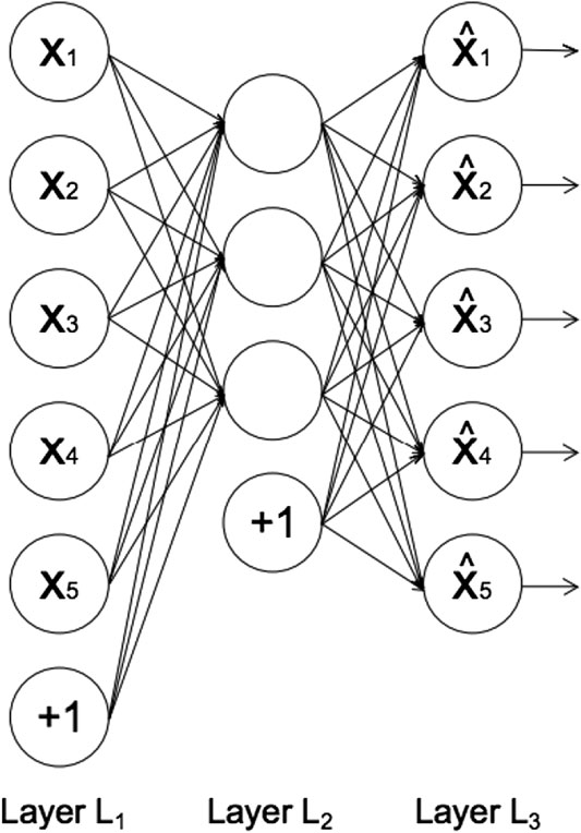
FIGURE 1. The architecture of an autoencoder, adapted from Sakurada and Yairi (2014). Each circle represents a neuron corresponding to a data-point. Layer L1 represents the input data, layer L2 the encoded data in latent space, and layer L3 the reconstructed data. The circles labeled “+1” are known as “bias units,” which are parameters that are adjusted during training to improve the performance of the neural network.

In feed-forward neural networks, such as autoencoders, each neuron computes the following sum:

$y={\displaystyle \sum }_i{w}_i{x}_i+b,(2)$

where x_i represents the input from the previous layer, w_i enotes the weights associated with the connections between neurons in different layers, and b denotes the bias term associated with each layer (represented by the circles labeled “+1” in Figure 1). The number of neurons in each layer defines the dimension of the data representation in that layer. The output of each neuron, f(y), is called the activation function. Rectified Linear Unit, (Hahnioser et al., 2000) is the most commonly used activation function due to its low computational cost (Agarap, 2018). The function is described as:

$f\left(y\right)=\max \left(0,y\right).(3)$

The sigmoid activation function (Chandra and Singh, 2004) is also commonly used. It is defined by:

$f\left(y\right)=\frac{1}{1+e^{-y}},(4)$

where y is defined in Eq. 2. Analysis of the use of various activation functions in the remit of plasma physics are given by Kube et al. (2019).

In order to improve the representation of the compressed data in layer L2 and minimize the discrepancy between the input and reconstruction layer, the autoencoder adjusts the weights and biases by minimising a loss function through an optimiser (described below). The binary cross-entropy loss function (de Boer et al., 2005) is typically used when the input data, x, are normalized to values between 0 and 1. The loss value, c, increases as the reconstruction data, $\widehat{x}$, diverge from the input data. The loss function is defined as:

$c=-\left[x\ln \left(\widehat{x}\right)+\left(1-x\right)\ln \left(1-\widehat{x}\right)\right].(5)$

An overview of various loss functions is provided by Janocha and Czarnecki (2017). Optimisers are used to ensure the autoencoder converges quickly to a minimum loss value by finding the optimum value of the weight, w_i, of each neuron. This is achieved by running multiple iterations with different weight values, known as gradient descent (Ruder, 2016). The weights are adjusted in each iteration, t, according to:

$w_t=w_{t-1}-\alpha \frac{\partial c}{\partial \omega },(6)$

where $\partial c/\partial \omega$ is the gradient, which is a partial derivative of the loss value with respect to the weight. The learning rate, α, updates all the weights simultaneously with respect to the gradient descent. This learning rate is randomly initialized between 0 and 1 by the Algorithm. A low learning rate results in a slower convergence to the global minimum loss value. However a too high value for the learning rate impedes the gradient descent (Eq. 6) from converging on the optimum weights. The Adadelta optimiser (Zeiler, 2012) is commonly used due to its rapid convergence to the minimum loss value and its ability to adapt the learning rate depending on each parameter. The optimiser updates each parameter, θ, according to:

$\Delta {\theta }_t=-\frac{\text{RMS}{\left[\Delta \theta \right]}_{t-1}}{\text{RMS}{\left[g\right]}_t}{g}_t,(7)$

where Δθ_t is the parameter update at the t-th iteration, g_t is the gradient of the parameters at the t-th iteration, and RMS is the root mean square. An overview of the various optimisers is provided by Khandelwal (2019).

1.1.2 Principal Component Analysis

PCA is a statistical procedure that, as well as autoencoders, also reduces the dimensionality of input data. The algorithm achieves this by transforming the input data from a large number of correlated variables to a smaller number of uncorrelated variables, known as principal components. These principal components account for most of the variation in the original input data, making them a useful tool in feature extraction.

Before the procedure, the original data, X₀, are represented by a (n × Q) matrix, where n is the number of observations and Q is the number of variables (also called dimensions). In the first step, the algorithm scales and centers the data:

$X=\left(X_0-{\overline{X}}_0\right)D^{-1},(8)$

where ${\overline{X}}_0$ contains the means of each of the variables, and D is a diagonal matrix that contains the scaling coefficient of each variable. Typically, D_ii = σ_i where σ_i is the standard deviation of variable with index i (Peerenboom et al., 2015). The algorithm then uses X to calculate the covariance matrix:

$C_X=\frac{1}{n-1}{X}^{T}X,(9)$

which measures the correlation between the different variables. The principal components are calculated as the eigenvectors, A, of the covariance matrix:

$C_X=AL{A}^T,(10)$

where L is a diagonal matrix containing the eigenvalues associated with A. These principal components are ordered in decreasing order, whereby the first principal components account for most of the variation in the input data. These input data are finally projected into the principal component space according to:

$Z=XA,(11)$

where Z represents the output data containing the principal component scores. The dimensionality of these output data are determined by the number of principal components used.

1.1.3 Mean Shift

The mean shift algorithm is a non-parametric clustering technique that is used for locating the maxima of a density function in a sample space. The algorithm aims to discover the number of clusters within a dataset, meaning no prior knowledge of the number of clusters is necessary.

For a dataset containing n data-points x_i, the algorithm starts finding each maximum of the dataset’s density function by randomly choosing a data-point to be the mean of the distribution, x. The algorithm then uses a kernel function, K, to determine the weights of the nearby data-points for re-estimating the mean. The variable h is the width of the kernel window. Typically, a Gaussian kernel, k, is used:

$K\left(\frac{x-x_i}{h}\right)=c_{k}k\left({\left|\left|\frac{x-x_i}{h}\right|\right|}^2\right)=\exp \left(-c_k{\left|\left|\frac{x-x_i}{h}\right|\right|}^2\right),(12)$

where c_k is the normalising constant. With the kernel function, the multivariate kernel density estimator is obtained:

$f\left(x\right)=\frac{1}{n{h}^d}{\displaystyle \sum }_{i=1}^{n}K\left(\frac{x-x_i}{h}\right),(13)$

where d is the dimensionality of the dataset. The gradient of the density estimator is then:

$\begin{array}{c}▽f\left(x\right)=\frac{2c_k}{n{h}^{d+2}}{\displaystyle \sum }_{i=1}^n\left(x_i-x\right)g\left({\left|\left|\frac{x-x_i}{h}\right|\right|}^2\right)\\ =\frac{2c_k}{n{h}^{d+2}}\left[{\displaystyle \sum }_{i=1}^{n}g\left({\left|\left|\frac{x-x_i}{h}\right|\right|}^2\right)\right]m_h\left(x\right),\end{array}(14)$

where $g\left(x\right)=-k^{\prime }\left(x\right)$. The first term is proportional to the density estimate at x, and the second term, $m_h\left(x\right)$, is:

$m_h\left(x\right)=\frac{{{{\displaystyle \sum }}^{\text{}}}_{i=1}^n{x}_{i}g\left({\left|\left|\frac{x-x_i}{h}\right|\right|}^2\right)}{{{{\displaystyle \sum }}^{\text{}}}_{i=1}^{n}g\left({\left|\left|\frac{x-x_i}{h}\right|\right|}^2\right)}-x,(15)$

which is the mean shift vector and points toward the direction of the maximum increase in density. The mean shift algorithm therefore iterates between calculating the mean shift vector, $m_h\left(x^t\right)$, and translating the kernel window:

$x^{t+1}=x^t+m_h\left(x^t\right),(16)$

where t is the iteration step. Once the window has converged to a point in feature space where the density function gradient is zero, the algorithm carries out the same procedure with a new window until all data-points have been assigned to a maximum in the density function.

1.1.4 Agglomerative Clustering

AC is a type of hierarchical clustering that uses a “bottom-up” approach, whereby each data-point is first assigned a different cluster. Then pairs of similar clusters are merged until the specified number of clusters has been reached. During each recursive step, the AC algorithm combines clusters typically using Ward’s criterion (Ward, 1963), which finds pairs of clusters that lead to the smallest increase in the total intra-cluster variance after merging. The increase is measured by a squared Euclidean distance metric:

$d_{ij}=d\left(C_i,C_j\right)=||C_i-{C_j||}^2,(17)$

where C_i represents a cluster with index i. The algorithm implements Ward’s criterion using the Lance–Williams formula (Lance and Williams, 1967):

$\begin{array}{c}d\left(C_i\cup C_j,C_k\right)=\frac{n_i+n_k}{n_i+n_j+n_k}d\left(C_i,C_k\right)\\ +\frac{n_j+n_k}{n_i+n_j+n_k}d\left(C_j,C_k\right)-\frac{n_k}{n_i+n_j+n_k}d\left(C_i,C_j\right),\end{array}(18)$

where C_i, C_j, and C_k are disjoint clusters with sizes n_i, n_j, and n_k, and $d\left(C_i{{\displaystyle \cup }}^{\text{}}{C}_j,C_k\right)$ is the squared Euclidean distance between the new cluster $C_i{{\displaystyle \cup }}^{\text{}}{C}_j$ and C_k. The clustering algorithm uses Eq. 18 to find the optimal pair of clusters to merge.

1.2 The Magnetotail

We use electron data from the magnetotail in order to test the effectiveness of our method. The magnetotail is traditionally divided into three different regions: the plasma sheet, the plasma sheet boundary layer, and the lobes (Hughes, 1995). These regions are defined by their plasma and magnetic field characteristics. The low temperature (∼85 eV) outermost northern and southern lobes are on open magnetic field lines which results in a much lower plasma density of ∼0.01 cm (Lui, 1987). The plasma sheet boundary layer exists on the reconnected magnetic field lines. This region forms the transition region in between the plasma sheet and the lobes, and is characterized by a population of field-aligned particles and a plasma β, which is the ratio of the plasma pressure to the magnetic pressure, of ∼0.1 (Lui, 1987).

The innermost plasma sheet typically contains a comparatively hot (∼4,250 eV) and isotropic plasma with a relatively high particle density of ∼0.01 cm⁻³. At the center of the plasma sheet is the thin neutral current sheet, which is characterized by a relatively high plasma β of ∼0, and a magnetic field strength of near zero (Lui, 1987). Although isotropic electron pitch angle distributions (PADs) are the most dominant in the plasma sheet, many cases of pitch angle anisotropy have also been found (e.g., Walsh et al., 2013; Artemyev et al., 2014; Liu et al., 2020). These intervals correspond to a colder and denser electron population and are linked to: cold anisotropic ionospheric outflows (Walsh et al., 2013), and a penetration of cold electrons from the magnetosheath near the flanks (Artemyev et al., 2014).

2 Method and Application

In this section, we detail the steps required to classify different regions within a space plasma environment using machine learning techniques. As an example, we classify Cluster-Plasma Electron and Current Experiment (PEACE, Johnstone et al., 1997; Fazakerley et al., 2010) data (Laakso et al., 2010) from the Earth’s magnetotail to showcase our method, as this allows us to compare to the Cluster-ECLAT (European Cluster Assimilation Technology) (Boakes et al., 2014) database for evaluation. The same method, however, can be applied to any plasma regime where energy and pitch angle measurements are available. Our steps are as follows:

• Data preparation: We obtain the Cluster-PEACE data from different magnetotail regions based on the Cluster-ECLAT database, and prepare the data for testing.

• Reducing dimensionality: We build our autoencoder and use the encoder part to reduce the dimensionality of each pitch angle and energy distribution by a factor of 10. We use a PCA algorithm to further compress each distribution to a set of coordinates in 3D space.

• Clustering: We apply the mean-shift algorithm to determine how many clusters exist within the compressed magnetotail electron data, and use an AC algorithm to separate the compressed dataset into this number of clusters. This allows us to determine how many plasma regimes exist within the overall dataset.

• Evaluation: We estimate the probabilities of the AC labels and compare our clustering results to the original ECLAT labels in order to evaluate our method.

2.1 Data Preparation

We prepare PEACE instrument data from the Cluster mission’s C4 spacecraft (Escoubet et al., 2001) to test and present our method. The Cluster mission comprises of four spacecraft, each spinning at a rate of 4 s⁻¹. The PEACE data have a 4 s time resolution and are constructed from two instantaneous PAD measurements per spin. Each of our distributions is a two-dimensional differential energy flux product containing twelve 15° wide pitch angle bins and 26 energy bins, spaced logarithmically between 93 eV and 24 keV. The dimensionality of each distribution is 312 (12 × 26). We normalize the differential energy flux linearly between 0 and 1 based on the maximum flux value in the dataset. An example of an individual differential energy flux distribution used in our analysis is shown in Figure 2. We correct for spacecraft potential with measurements from the Cluster-EFW (Electric Field and Wave Experiment) instrument (Gustafsson et al., 2001) and corrections (19% increase) according to the results of Cully et al. (2007).

FIGURE 2

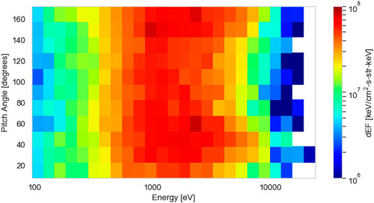
FIGURE 2. An example two-dimensional electron differential energy flux distribution, as a function of pitch angle (°) and energy (eV), measured by the Cluster-Plasma Electron and Current Experiment instrument in the magnetotail across a 4 s window (09:51:23–09:51:27 on October 13, 2003).

The ECLAT dataset consists of a detailed list of plasma regions encountered by each of the four Cluster spacecraft in the nightside magnetosphere. The dataset is available from July to October during the years 2001–2009. Using plasma and magnetic field moments from the PEACE, Cluster Ion Spectrometry (CIS) (Rème et al., 2001), and Fluxgate Magnetometer (FGM) (Balogh et al., 1997) instruments, the dataset provides a list of (inner and outer) plasma sheet, boundary layer, and lobe times. These regions are identified based on the plasma β, the magnetic field measurements, and the current density vectors. A comprehensive account of the ECLAT identification routine for each plasma region is provided by Boakes et al. (2014). To ensure that we test our method on a large number of data from each of the magnetotail regions (>50,000 samples), we obtain PEACE data from times when the C4 spacecraft has spent at least 1 h in each region, according to ECLAT.

2.2 Reducing Dimensionality

After preparing the dataset to include a series of >50,000 time intervals, each with its associated 2D pitch angle and energy distributions (e.g., Figure 2), the first step toward reducing the dataset’s dimensionality is to build a suitable autoencoder (described in Section 1.1.1). We construct our autoencoder using the Keras library. This step requires defining the number of neurons in each layer. The input and reconstruction layer should have the same number, which is equal to the dimensionality of the original dataset (312 for each time interval in this example). The middle encoded layer typically contains a compressed representation of the data that is by a factor of 10 smaller than the input data (Hinton and Salakhutdinov, 2006). We therefore specify our encoded layer to contain 32 neurons. The next step involves specifying the activation function for the neurons in the first and middle layers. We use the standard Rectified Linear Unit activation function (Hahnioser et al., 2000) in the encoder part of our autoencoder and the sigmoid activation function (Chandra and Singh, 2004) in the decoder part, as this function is used to normalize the output between 0 and 1.

The next step defines which loss function and optimiser the autoencoder uses in order to representatively compress and reconstruct the input data. As we use normalized output data, we choose the standard binary cross-entropy loss function (de Boer et al., 2005). In terms of the optimiser, we utilize the Adadelta optimiser (Zeiler, 2012) due to its speed and versatility. All of the activation functions, loss functions, and optimisers are available in the Keras library.

In the next step, we set the hyperparameters used for training the autoencoder. These hyperparameters include: the number of epochs, the batch size, and the validation split ratio. The number of epochs represents the number of training iterations undergone by the autoencoder, with the weights and biases updated at each iteration. The batch size defines the number of samples that are propagated through the network at each iteration. It is equal to 2ⁿ, where n is a positive integer. The batch size (256 in our case) is ideally set as close to the dimensionality of the input data as possible. The validation split ratio determines the percentage of the input data that should remain “unseen” by the autoencoder in order to verify that the algorithm is not overfitting the remaining training data. We set the validation split ratio to 1/12, which is commonly used for large datasets (Guyon, 1997). At each iteration, a training loss value and a validation loss value are produced, which are determined by the binary cross-entropy loss function. Both of these values converge to their minima after a certain number of iterations, at which point the autoencoder cannot be optimized to the input data any further. Loss values <0.01 are typically considered ideal (Le et al., 2018).

After retrieving the compressed representation of the input data from the encoding layer (with a dimensionality of 32 in our case), we apply a PCA algorithm (see Section 1.1.2) to the compressed data to reduce the dimensionality to 3. We obtain the PCA algorithm from the scikit-learn library. We set the output dimensionality of the PCA algorithm to 3 as the following clustering algorithms used in this method are computationally expensive and their performance scales poorly with increasing dimensionality (Lukasovã, 1979; Comaniciu and Meer, 2002). Setting the dimensionality to 3 has the added benefit that the clusters can be visualised.

2.3 Clustering

Once the dimensionality reduction stage has taken place and each pitch angle and energy distribution is represented by three PCA values, we use clustering algorithms to separate the dataset into the different particle populations. To first determine how many populations exist within the dataset (8 in our case), we apply a mean shift clustering algorithm (see Section 1.1.3) to the data to find the number of maxima, n_c, in the distribution of data-points. We obtain the mean shift algorithm from the scikit-learn library. We set the bandwidth, represented by h in Eq. 15 to 1, which we find optimizes the time taken for the algorithm to converge on the maxima in the density distribution.

After determining the number of clusters in the dataset, we use an AC algorithm (see Section 1.1.4) to assign each data-point to one of the clusters. We obtain the AC algorithm from the scikit-learn library and instantiate the algorithm by specifying the number of clusters, n_c, before applying it to the compressed dataset. Assigning several clusters to a large dataset with three dimensions is a computationally expensive task, however we find the AC algorithm converges relatively quickly in comparison to other clustering algorithms. A further advantage of the hierarchical clustering procedure, used in the AC algorithm, is that data-points belonging to a single non-spherical structure in the 3-dimensional parameter space are not incorrectly separated into different clusters, unlike the more widely used K-means algorithm (Arthur, 2007).

Figure 3 contains a flow diagram detailing our method.

FIGURE 3

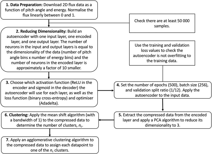
FIGURE 3. Flow diagram illustrating the steps we take to reduce the dimensionality of the dataset and subsequently apply clustering algorithms to characterize the different populations. Our choices for the functions and input parameters necessary to train the autoencoder are shown in brackets in steps 3 and 4.

2.4 Evaluation

Figure 4 shows the training and validation loss values associated with each iteration during the training of our autoencoder. We use this graph to check if the autoencoder is overfitting to the training data, which is evident if the training loss starts to decrease more rapidly than the validation loss. In this case, our autoencoder is not overfitting at any iteration during training. Figure 4 shows that both the loss values start to rapidly level off in less than 100 epochs. Both loss values, however, continue to decrease, with the training loss value converging to 0.0743 after 444 iterations, and the validation loss value converging to 0.0140 after 485 iterations. We therefore set the number of epochs to 500. As both loss values are lower than 0.01, we conclude the autoencoder is accurately reconstructing both sets of input data, assuring us that the encoded data with a lower dimensionality is representative of the original 2D distribution functions. The lower validation loss than training loss in Figure 4 indicates the presence of anomalous data in the training set that is not represented in the validation set. We discuss this anomalous data later in this section.

FIGURE 4

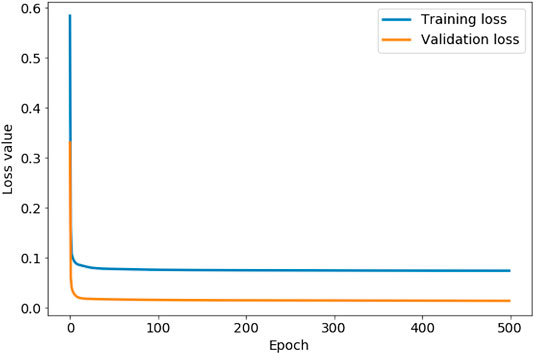
FIGURE 4. The evolution of the training loss value and validation loss value as the autoencoder iterates through 500 steps (epochs).

Figure 5 shows the result of applying the AC algorithm to the compressed magnetotail electron data after the implementation of the autoencoder and PCA algorithms. The 3-dimensional representation shows that the clustering algorithm is able to assign data-points of varying PCA values to the same cluster if they belong to the same complex non-spherical structure, e.g., clusters 0, 4, and 6. The clustering algorithm is able to form clear boundaries between clusters with adjacent PCA values, e.g., between clusters 0, 1, and 7, with no mixing of cluster labels on either side of the boundaries. The clustering algorithm locates the boundaries by finding areas with a low density of data-points in comparison to the centers of the clusters.

FIGURE 5

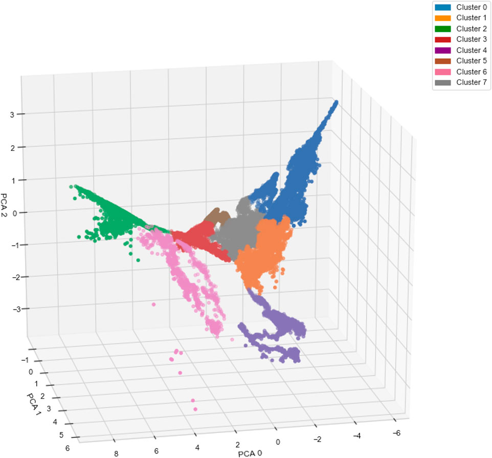
FIGURE 5. Three-dimensional representation of the magnetotail data after undergoing dimensionality reduction via an autoencoder and principal component analysis (PCA) algorithm. The colors represent the clustering results from the agglomerative clustering algorithm.

Figure 6 shows the results of averaging the 2D differential energy flux distributions in pitch angle and energy space for each of the eight clusters. Using moments data collected by the PEACE, FGM, and CIS instruments, we compare the proton plasma βs, electron densities and temperatures, and magnetic field strengths to the average 2D distribution of each cluster. This process allows us to verify the consistency of the clustering method and provide general region classifications in order to make comparisons with the ECLAT labels. Our classifications (shown in the captions below each sub-figure) are produced with the aid of previous analyses of electron PADs (e.g., Walsh et al., 2011; Artemyev et al., 2014) and the plasma and magnetic field parameters (e.g., Lui, 1987; Artemyev et al., 2014) in the magnetotail.

FIGURE 6

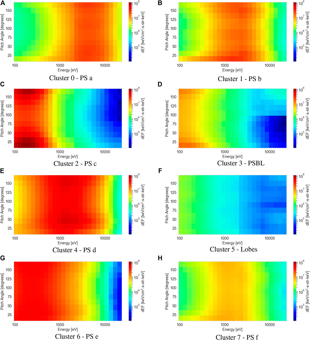
FIGURE 6. Average electron differential energy flux distributions as a function of pitch angle and energy for each of the eight clusters (A-H) classified by the agglomerative clustering algorithm. Each cluster is assigned a magnetotail region (included in the subcaptions) based on our interpretation of their plasma and magnetic field parameters.

The individual sub-figures in Figure 6 display large differences in the average electron 2D pitch angle and energy distributions. Each average distribution differs by either: the energy of the peak flux, the peak value of the flux, or the amount of pitch angle anisotropy, i.e., the difference in flux between the parallel and perpendicular magnetic field direction. The lack of identical average distributions amongst the clusters shows the mean shift algorithm has not overestimated the number of clusters. By observing the individual 2D distributions within each cluster, we see a distinct lack of intra-cluster variance, showing the mean shift algorithm does not underestimate the number of clusters.

A limitation of using the AC algorithm is that outliers or anomalous data are not differentiated from the main clusters. Clustering a sizable number of outliers with the main populations can lead to ambiguity in the defining characteristics of each population, reducing the robustness of our method. In our case, Figure 5 shows only nine data points, within cluster 6, that are disconnected from the main structure of cluster 6 due to their distinct PCA values. We observe similar phenomenon to a lesser extent with cluster 2. To counteract this issue, we perform an outlier detection procedure using the reconstructed output of the autoencoder. By calculating the mean square error (MSE) between each input data-point and its reconstructed output, we isolate outliers in the dataset from the AC analysis based on their large MSE values, in comparison to 99.95% of the data-points. During training, the autoencoder learns the latent space representation that defines the key characteristics of the bulk populations present in the dataset. The most relevant features of an anomalous particle distribution are not present in this subspace, resulting in a large MSE between the reconstructed data, which lacks these important features, and the original data. This technique effectively identifies the nine obvious outliers observable by eye in Figure 5, along with six from cluster 2 and 5 from cluster 1.

We use Gaussian mixture models (GMMs, McLachlan and Peel, 2000) to establish the probabilities of each of the data-points belonging to the clusters they have been assigned to by the AC algorithm, providing useful information on the uncertainty associated with our region classification method. We obtain the GMM from the scikit-learn library. For each data-point, x_i, a GMM fits a normal distribution, $\mathcal{N}$, to each cluster and computes the sum of probabilities as:

$p\left(x_i\right)=\underset{j=1}{{\displaystyle \sum }^k}{\varphi }_j\mathcal{N}\left(x_i;{\mu }_j,{\tau }_j\right)=1,(19)$

where µ_j and τ_j are the mean and covariance of the normal distribution belonging to cluster j, and ${\varphi }_j$ is the mixing coefficient which represents the weight of Gaussian j and is calculated by the Expectation–Maximisation algorithm (Dempster et al., 1977). A complete description of GMMs and the Expectation–Maximisation algorithm is provided by Dupuis et al. (2020).

Figure 7 shows a histogram of the probabilities, calculated by the GMM, associated with each data-point belonging to the cluster it is assigned to by the AC algorithm. More than 92% of the data-points have a probability of over 0.9, and <1% of the data-points have a probability of <0.5. This indicates a high certainty in our clustering method and validates the high precision in our region classifications. Further investigations of the data-points with associated probabilities of <0.5 show that these data-points exist on the boundary between clusters 0 and 1, i.e., two plasma sheet populations that differ by temperature. This illustrates a small limitation in the AC method when distinguishing between relatively similar plasma regimes.

FIGURE 7

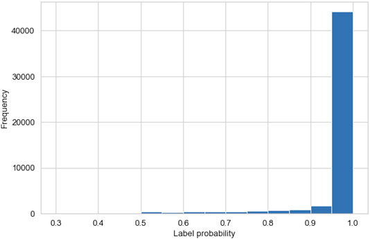
FIGURE 7. Histogram showing the probabilities, generated by Gaussian mixture model (GMMs), that the data-points belong to the cluster assigned to them by the agglomerative clustering algorithm.

Table 1 shows the median and upper and lower quartiles of the electron density, electron temperature, magnetic field, and ion plasma β for each of the eight clusters designated by our AC algorithm. None of the eight clusters have comparable median and quartile values across all four of the chosen parameters. Certain pairs of clusters exhibit similarities in the median and quartile values for one or two of the four parameters, e.g., clusters 0 and 4 exhibit similar electron densities and magnetic field strengths, and clusters 3 and 6 exhibit similar magnetic field strengths. However there are large differences in the values of the remaining parameters for these pairs of clusters. These results show that clear differences in the 2D pitch angle and energy distributions (see Figure 6) can translate into distinctions between certain but not all plasma parameter measurements, providing a strong indicator that full 2D distributions can effectively be used to distinguish between similar particle populations. Regarding the ECLAT classifications, which are based on magnetic field and plasma β measurements, certain pairs of clusters exhibit a similar range of values in both of these measurements, e.g., clusters 0 and 4 and clusters 1 and 7. As the majority of data-points for all of these clusters are considered the same plasma sheet population by ECLAT (see Table 2), we conclude that using a limited number of parameters to provide classifications overlooks distinctions between different populations and incorrectly groups them into the same category.

TABLE 1

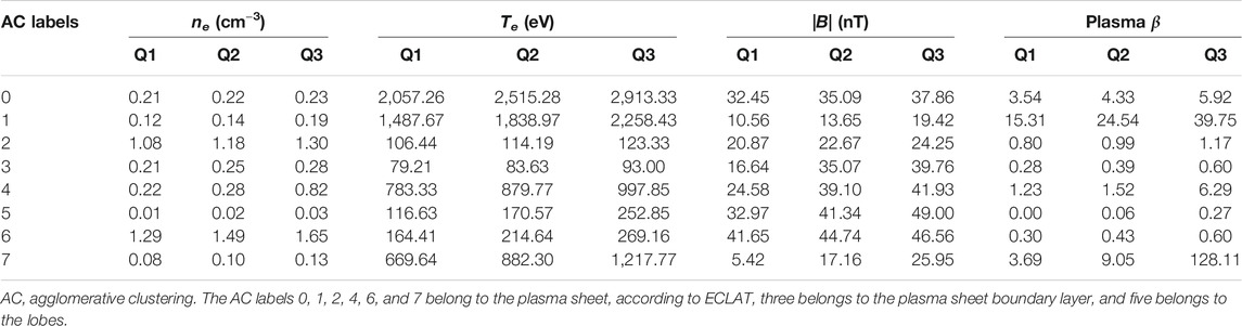
TABLE 1. Comparisons of the median, Q2, and upper, Q3, and lower, Q1, quartile values of the electron density n_e, electron temperature T_e, magnetic field |B|, and plasma β associated with each of the eight clusters.

TABLE 2

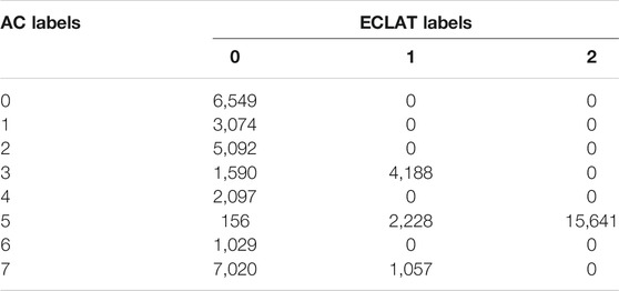
TABLE 2. Contingency table comparing the agglomerative clustering (AC) labels of the magnetotail electron data to the original ECLAT labels (0 = PS, 1 = PSBL, and 2 = lobes).

Table 2 shows our comparison between the eight AC labels and the region names given in the ECLAT database, for the magnetotail data used in our example.

In Table 2, there is some disagreement with three of our clusters, namely AC labels 3, 5, and 7, which correspond to the plasma sheet boundary layer, the lobes, and a plasma sheet population respectively. However for each of these clusters, the majority of labels are in agreement with the ECLAT regions (72.4, 86.8, and 86.9% for AC clusters 3, 5, and 7 respectively). For AC labels 0, 1, 2, 4, and 6, which represent various other populations within the plasma sheet, there is 100% agreement with the ECLAT label 0, which denotes the plasma sheet. By using this method to characterize full electron pitch angle and energy distributions, instead of using the derived moments, we are successfully able to distinguish between multiple populations within what has historically been considered as one region, due to the lack of variation in the plasma moments (see Table 1) as well as the similarity in spatial location. Using 2D pitch angle and energy distributions also improves the time resolution of the plasma region classifications, due to a higher cadence in the spacecraft flux and counts data (e.g., 4 s resolution for the PEACE instrument) in comparison to the moments data (e.g., 8 s resolution for CIS moments and 16 s resolution for PEACE moments).

3 Conclusion

We present a novel machine learning method that characterizes full particle distributions in order to classify different space plasma regimes. Our method uses autoencoders and subsequently PCA to reduce the dimensionality of the 2D particle distributions to three dimensions. We then apply the mean shift algorithm to discover the number of populations in the dataset, followed by the AC algorithm to assign each data-point to a population.

To illustrate the effectiveness of our method, we apply it to magnetotail electron data and compare our results to previous classifications, i.e. the ECLAT database, that utilizes moments. With our method, we find multiple distinct electron populations within the plasma sheet, which previous studies have identified as one region (Table 2). These findings show that key features in particle distributions are not fully characterized by the plasma moments (e.g., Table 1), resulting in important distinctions between populations being overlooked. For example, we find two separate cold dense anisotropic populations in the plasma sheet (clusters 2 and 6), which are less abundant than the hotter and more isotropic plasma sheet populations. By using our clustering method to specify an exact list of times when populations like these are observed, we create a more comprehensive picture of their spatial distribution. Inherent time-dependencies may also contribute to our finding of multiple plasma sheet populations. Even in this case, our method is effective in characterising the evolution of particle populations, made possible by the high time resolution of our region classifications. In a follow up study, we will use this information to link the occurrence of these populations to other high-resolution spacecraft measurements in different plasma regions, in order to understand the physical processes driving changes in the less abundant particle populations. As an example analysis, our high resolution classifications of the observed anisotropic plasma sheet populations could be combined with previous theories on the sources of these populations (e.g., Walsh et al., 2013; Artemyev et al., 2014), to understand the relative contributions of particle outflows from distinct magnetospheric regions, such as the magnetosheath or ionosphere.

Comparisons between this original method and the previous classifications from ECLAT also show specific periods of disagreement (e.g., we classify a small number of ECLAT periods of plasma sheet as the plasma sheet boundary layer). This discrepancy shows that using the full 2D pitch angle and energy distributions, without requiring prior assumptions about magnetospheric plasma regions, may redefine the classifications of electron populations, along with our understanding of their plasma properties. Our method, which uses open-source and easily accessible machine learning techniques, can be used to better characterize any space plasma regime with sufficient in-situ observations. By not being constrained to a small number of parameters, this method allows for a more complete understanding of the interactions between various thermal and non-thermal populations. With increasingly large datasets being collected by multi-spacecraft missions, such as Cluster (Escoubet et al., 2001) (>10⁹ full distributions in 20 years) and Magnetospheric Multiscale Mission (Sharma and Curtis, 2005), similar methods would provide a useful tool to reduce the dimensionality of distributions, thereby optimising data retrieval on Earth. Furthermore, combining this method with large-scale survey data, such as NASA/GSFC’s OMNI database, would allow users to isolate a specific population or plasma region for analysis of its properties.

Data Availability Statement

Publicly available datasets were analyzed in this study. This data can be found here: The datasets analysed in this study can be found in the Cluster Science Archive (https://csa.esac.esa.int/csa-web/).

Author Contributions

MRB developed the method described in the manuscript, tested it on the magnetotail data and wrote the manuscript. IJR was the lead supervisor who guided the direction of the project and provided insight at every stage. AW provided expertize on the magnetotail and the various populations that we observed, aiding the evaluation of our method. DV was also important in classifying the plasma regimes and provided insights into the physical processes governing electrons in space plasmas. AWS was key to the development of the method due to his expertize in machine learning. All co-authors made important contributions to the manuscript.

Funding

MB is supported by a UCL Impact Studentship, joint funded by the ESA NPI program. IR the STFC Consolidated Grant ST/S000240/1 and the NERC grants NE/P017150/1, NE/P017185/1, NE/V002554/1, and NE/V002724/1. DV is supported by the STFC Consolidated Grant ST/S000240/1 and the STFC Ernest Rutherford Fellowship ST/P003826/1. AS is supported by the STFC Consolidated Grant ST/S000240/1 and by NERC Grants NE/P017150/1 and NE/V002724/1.

Conflict of Interest

The authors declare that the research was conducted in the absence of any commercial or financial relationships that could be construed as a potential conflict of interest.

Acknowledgments

We thank the Cluster instrument teams (PEACE, FGM, CIS, EFW) for the data used in this study, in particular the PEACE operations team at the Mullard Space Science Laboratory. We also acknowledge the European Union Framework 7 Program, the ECLAT Project FP7 Grant No. 263325, and the ESA Cluster Science Archive.

References

Abdi, H., and Williams, L. J. (2010). Principal component analysis. WIREs Comput. Stat. 2, 433–459. doi:10.1002/wics.101

CrossRef Full Text | Google Scholar

Agarap, A. F. (2018). Deep learning using rectified linear units (ReLU). arXiv:1803.08375.

Google Scholar

Artemyev, A. V., Walsh, A. P., Petrukovich, A. A., Baumjohann, W., Nakamura, R., and Fazakerley, A. N. (2014). Electron pitch angle/energy distribution in the magnetotail. J. Geophys. Res. Space Phys. 119, 7214–7227. doi:10.1002/2014JA020350

CrossRef Full Text | Google Scholar

Arthur, D. (2007). “k-means++: the advantages of careful seeding,” in Proceedings of the eighteenth annual ACM-SIAM symposium on discrete algorithms, New Orleans, United States, January 7, 2007. 1027–1035

Google Scholar

Balogh, A., Dunlop, M. W., Cowley, S. W. H., Southwood, D. J., Thomlinson, J. G., Glassmeier, K. H., et al. (1997). The cluster magnetic field investigation. Space Sci. Rev. 79, 65–91. doi:10.1023/A:1004970907748

CrossRef Full Text | Google Scholar

Bishop, C. M. (1998). “Bayesian PCA,” in Proceedings of the 11th international conference on neural information processing systems, Denver, United States, December 1, 1997. (Cambridge, MA: MIT Press), 382–388.

Google Scholar

Boakes, P. D., Nakamura, R., Volwerk, M., and Milan, S. E. (2014). ECLAT cluster spacecraft magnetotail plasma region identifications (2001–2009). Dataset Papers Sci. 2014, 684305. doi:10.1155/2014/684305

CrossRef Full Text | Google Scholar

Chandra, B., and Sharma, R. K. (2014). “Adaptive noise schedule for denoising autoencoder,” in Neural information processing. Editors C. K. Loo, K. S. Yap, K. W. Wong, A. Teoh, and K. Huang (Berlin, Germany: Springer International Publishing), 535–542.

Google Scholar

Chandra, P., and Singh, Y. (2004). An activation function adapting training algorithm for sigmoidal feedforward networks. Neurocomputing 61, 429–437. doi:10.1016/j.neucom.2004.04.001

CrossRef Full Text | Google Scholar

Chollet, F., Allison, K., Wicke, M., Bileschi, S., Bailey, B., Gibson, A., et al. (2015). Keras. Available at: https://keras.io (Accessed February 15, 2020).

Google Scholar

Comaniciu, D., and Meer, P. (2002). Mean shift: a robust approach toward feature space analysis. IEEE Trans. Pattern Anal. Machine Intell. 24, 603–619. doi:10.1109/34.1000236

CrossRef Full Text | Google Scholar

Cully, C. M., Ergun, R. E., and Eriksson, A. I. (2007). Electrostatic structure around spacecraft in tenuous plasmas. J. Geophys. Res. Atmos. 112, A09211. doi:10.1029/2007JA012269

CrossRef Full Text | Google Scholar

de Boer, P.-T., Kroese, D. P., Mannor, S., and Rubinstein, R. Y. (2005). A tutorial on the cross-entropy method. Ann. Oper. Res. 134, 19–67. doi:10.1007/s10479-005-5724-z

CrossRef Full Text | Google Scholar

Dempster, A. P., Laird, N. M., and Rubin, D. B. (1977). Maximum likelihood from incomplete data via the EM algorithm. J. R. Stat. Soc. Ser. B Methodol. 39, 1–22. doi:10.1111/j.2517-6161.1977.tb01600.x

CrossRef Full Text | Google Scholar

Dupuis, R., Goldman, M. V., Newman, D. L., Amaya, J., and Lapenta, G. (2020). Characterizing magnetic reconnection regions using Gaussian mixture models on particle velocity distributions. Astrophys J. 889, 15. doi:10.3847/1538-4357/ab5524

Google Scholar

Escoubet, C. P., Fehringer, M., and Goldstein, M. (2001). Introduction: the cluster mission. Ann. Geophys. 19, 1197–1200. doi:10.5194/angeo-19-1197-2001

CrossRef Full Text | Google Scholar

Fazakerley, A. N., Lahiff, A. D., Wilson, R. J., Rozum, I., Anekallu, C., West, M., et al. (2010). “Peace data in the cluster active archive,” in The cluster active archive. Editors Laakso, H., Taylor, M., and Escoubet, C. P. (Dordrecht, Netherlands: Springer Netherlands), 129–144.

Google Scholar

Fukunaga, K., and Hostetler, L. (1975). The estimation of the gradient of a density function, with applications in pattern recognition. IEEE Trans. Inf. Theory. 21, 32–40. doi:10.1109/tit.1975.1055330

CrossRef Full Text | Google Scholar

Gustafsson, G., André, M., Carozzi, T., Eriksson, A. I., Fälthammar, C.-G., Grard, R., et al. (2001). First results of electric field and density observations by Cluster EFW based on initial months of operation. Ann. Geophys. 19, 1219–1240. doi:10.5194/angeo-19-1219-2001

CrossRef Full Text | Google Scholar

Guyon, I. (1997). A scaling law for the validation-set training-set size ratio. Murray Hill, NJ: AT & T Bell Laboratories.

Google Scholar

Hahnioser, R., Sarpeshkar, R., Mahowald, M., Douglas, R., and Seung, H. (2000). Digital selection and analogue amplification coexist in a cortex- inspired silicon circuit. Nature 405, 947–951. doi:10.1038/35016072

CrossRef Full Text | Google Scholar

Hapgood, M., Perry, C., Davies, J., and Denton, M. (2011). The role of suprathermal particle measurements in crossscale studies of collisionless plasma processes. Planet. Space Sci. 59, 618–629. doi:10.1016/j.pss.2010.06.002

CrossRef Full Text | Google Scholar

Hinton, G. E., and Salakhutdinov, R. R. (2006). Reducing the dimensionality of data with neural networks. Science 313, 504–507. doi:10.1126/science.1127647

CrossRef Full Text | Google Scholar

Hughes, W. J. (1995). “The magnetopause, magnetotail, and magnetic reconnection,” in Introduction to space physics. Editors Kivelson, M. G., and Russell, C. T. (Cambridge, UK: Cambridge University Press), Chap. 9, 227–288.

Google Scholar

Janocha, K., and Czarnecki, W. M. (2017). On loss functions for deep neural networks in classification. arXiv.

Google Scholar

Johnstone, A. D., Alsop, C., Burge, S., Carter, P. J., Coates, A. J., Coker, A. J., et al. (1997). Peace: a plasma electron and current experiment. Dordrecht, Netherlands: Springer Netherlands, 351–398

Google Scholar

Khandelwal, R. (2019). Overview of different optimizers for neural networks. Available at: https://medium.com/datadriveninvestor/overview-of-different-optimizers-for-neural-networks-e0ed119440c3. (Accessed July 7, 2020).

Google Scholar

Kube, R., Bianchi, F. M., Brunner, D., and LaBombard, B. (2019). Outlier classification using autoencoders: application for fluctuation driven flows in fusion plasmas. Rev. Sci. Instrum. 90, 013505. doi:10.1063/1.5049519

CrossRef Full Text | Google Scholar

Laakso, H., Perry, C., McCaffrey, S., Herment, D., Allen, A. J., Harvey, C. C., et al. (2010). “Cluster active archive: Overview,” in The cluster active archive. Editors Laakso, H., Taylor, M., and Escoubet, C. P. (Dordrecht, Netherlands: Springer Netherlands), 3–37

Google Scholar

Lance, G. N., and Williams, W. T. (1967). A general theory of classificatory sorting strategies: 1. Hierarchical systems. Comput. J. 9, 373–380. doi:10.1093/comjnl/9.4.373

CrossRef Full Text | Google Scholar

Le, L., Patterson, A., and White, M. (2018). “Supervised autoencoders: improving generalization performance with unsupervised regularizers,” in Advances in neural information processing systems (Red Hook, NY: Curran Associates, Inc.), Vol. 31, 107–117.

Google Scholar

Liu, C. M., Fu, H. S., Liu, Y. Y., Wang, Z., Chen, G., Xu, Y., et al. (2020). Electron pitch-angle distribution in earth’s magnetotail: pancake, cigar, isotropy, butterfly, and rolling-pin. J. Geophys. Res. Space Phys. 125, e2020JA027777. doi:10.1029/2020JA027777

CrossRef Full Text | Google Scholar

Lui, A. T. Y. (1987). Road map to magnetotail domains. Baltimore, MD: John Hopkins University Press, 3–5.

Google Scholar

Lukasovã, A. (1979). Hierarchical agglomerative clustering procedure. Pattern Recogn. 11, 365–381. doi:10.1016/0031-3203(79)90049-9

CrossRef Full Text | Google Scholar

McLachlan, G., and Peel, D. (2000). ML fitting of mixture models. Hoboken, NJ: John Wiley & Sons, Ltd., Chap. 2, 40–80. doi:10.1002/0471721182.ch2

CrossRef Full Text | Google Scholar

Øieroset, M., Lin, R. P., Phan, T. D., Larson, D. E., and Bale, S. D. (2002). Evidence for electron acceleration up to ∼300 keV in the magnetic reconnection diffusion region of earth’s magnetotail. Phys. Rev. Lett. 89, 195001. doi:10.1103/PhysRevLett.89.195001

CrossRef Full Text | Google Scholar

Pedregosa, F., Varoquaux, G., Gramfort, A., Michel, V., Thirion, B., Grisel, O., et al. (2011). Scikit-learn: machine learning in Python. J. Mach. Learn. Res. 12, 2825–2830. doi:10.5555/1953048.2078195

Google Scholar

Peerenboom, K., Parente, A., Kozák, T., Bogaerts, A., and Degrez, G. (2015). Dimension reduction of non-equilibrium plasma kinetic models using principal component analysis. Plasma Sources Sci. Technol. 24, 025004. doi:10.1088/0963-0252/24/2/025004

CrossRef Full Text | Google Scholar

Rème, H., Aoustin, C., Bosqued, J. M., Dandouras, I., Lavraud, B., Sauvaud, J. A., et al. (2001). First multispacecraft ion measurements in and near the Earth’s magnetosphere with the identical Cluster ion spectrometry (CIS) experiment. Ann. Geophys. 19, 1303–1354. doi:10.5194/angeo-19-1303-2001

CrossRef Full Text | Google Scholar

Ruder, S. (2016). An overview of gradient descent optimization algorithms. arXiv e-prints.

Google Scholar

Sakurada, M., and Yairi, T. (2014). “Anomaly detection using autoencoders with nonlinear dimensionality reduction,” in Proceedings of the MLSDA 2014 2nd workshop on machine learning for sensory data analysis, Gold Coast, Australia, December 2, 2014. (New York, NY: Association for Computing Machinery), 4–11. doi:10.1145/2689746.2689747

CrossRef Full Text | Google Scholar

Sharma, A. S., and Curtis, S. A. (2005). Magnetospheric multiscale mission. Dordrecht, Netherlands: Springer Netherlands, 179–195. doi:10.1007/1-4020-3109-28

CrossRef Full Text | Google Scholar

Walsh, A. P., Fazakerley, A. N., Forsyth, C., Owen, C. J., Taylor, M. G. G. T., and Rae, I. J. (2013). Sources of electron pitch angle anisotropy in the magnetotail plasma sheet. J. Geophys. Res. Space Phys. 118, 6042–6054. doi:10.1002/jgra.50553

CrossRef Full Text | Google Scholar

Walsh, A. P., Owen, C. J., Fazakerley, A. N., Forsyth, C., and Dandouras, I. (2011). Average magnetotail electron and proton pitch angle distributions from cluster PEACE and CIS observations. Geophys. Res. Lett. 38, 1029. doi:10.1029/2011GL046770

CrossRef Full Text | Google Scholar

Ward, J. H. (1963). Hierarchical grouping to optimize an objective function. J. Am. Stat. Assoc. 58, 236–244. doi:10.1080/01621459.1963.10500845

CrossRef Full Text | Google Scholar

Zeiler, M. D. (2012). Adadelta: an adaptive learning rate method. arXiv e-prints.

Google Scholar