A Review of Studies of Geomagnetic Storms and Auroral/Magnetospheric Substorms Based on the Electric Current Approach

Introduction

There were at least three fields: geomagnetism, auroral (optical) physics, and ionospheric physics. The three fields were almost independently developed until 1960. Satellites were introduced at that time and helped to combine these three fields to establish a new field of science, space physics. It was soon realized that one of the major tasks in space physics was to study how the magnetosphere generates geomagnetic storms and substorms (output) by varying solar wind intensity (input) or how the magnetosphere responds after receiving energy from the solar wind and converts it into two phenomena, geomagnetic storms and auroral/magnetospheric substorms, Figure 1.

FIGURE 1

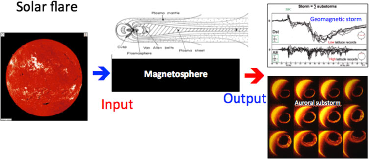
FIGURE 1. A schematic presentation, indicating the role of the magnetosphere, receiving solar wind disturbances as the input and producing geomagnetic storms and auroral substorms as the output.

This article presents a historical review of space physics from its birth around 1960. Instead of a textbook-like way, I have decided to describe the history based mostly on my own experience. I will describe what kind of problems I encountered and how I tried to solve them and how I succeeded or failed. It is hoped that my humble experience will be useful for younger generations, although it is admittedly a one-side view.

The Earliest Days

Our field of science had a rocky start. Carrington was the first person who observed a solar flare on September 2, 1859 (a white light flare, of the most intense type). Carrington confirmed this “abnormal” phenomenon by a magnetic observation and noted a possible association between them by stating: “One swallow does not make a summer”. However, his work got the attention of Lord Kelvin in 1889, who claimed that “It seems as if we may also be forced to conclude that the supposed connection between magnetic storm and sunspots is unreal and that seeming agreement between the periods has been mere coincidence” ; he stated also that the event is “a fifty years” outstanding difficulty.”

Maunder (1905), an observer at the Greenwich Astronomical Observatory, took up this subject by observing the so-called “27-day recurrence tendency” of geomagnetic storms and concluded the following:

First: The origin of our magnetic disturbances lies in the Sun.

Second: The areas of the Sun giving rise to our magnetic disturbances are definite and restricted areas.

Third: The areas of the Sun wherein these magnetically active areas are situated rotate with the Sun.

His statement was the first one to find the solar-terrestrial relationship based on the observations of solar flares and geomagnetic storms together, but was greeted immediately as “the mystery is left more mysterious than ever” by Schuster (1911) and some others. One lesson here is that observational facts, if correctly interpreted, can overcome authoritative criticisms such as by Kelvin.

Lord Kelvin did not consider that solar magnetic field changes can be observed at the distance of the Earth, but was not aware that solar gases (streams and coronal mass ejections (CMEs)) can carry effects of solar flares all the way to the Earth.

On the other hand, at the present time, we should be aware of the fact that we are still uncertain about processes associated with solar flares, how they eject CMEs and how the coronal hole causes streams, as well as why and how the solar wind blows and why the corona has a very high temperature. These are areas in which solar physicists and space physicists can work together. In fact, this is one area in which space physicists are capable of contributing to with their background.

At that time, both Birkeland (1918) and Stormer (1955) considered that auroras were caused by a beam of electrons from the Sun; electrons were discovered in 1897. Birkeland had the well-known Terella experiment, and Stormer made an extensive calculation of the trajectories of electron beams from the Sun to the Earth's dipole field.

Chapman’s Study of the Formation of the Magnetosphere

Chapman (1918) made statistically a comprehensive study of geomagnetic storms and established the present standard concept of geomagnetic storms; most geomagnetic storms begin with a step function-like increase in the horizontal (H) component of about 25 nT (called the sudden commencement, ssc), which is followed by a relatively quiet period of a few hours, called initial phase, and then the main phase, a decrease of the H component of more than 100 nT for several hours. After the main phase, the H component slowly recovers (Figure 2).

FIGURE 2

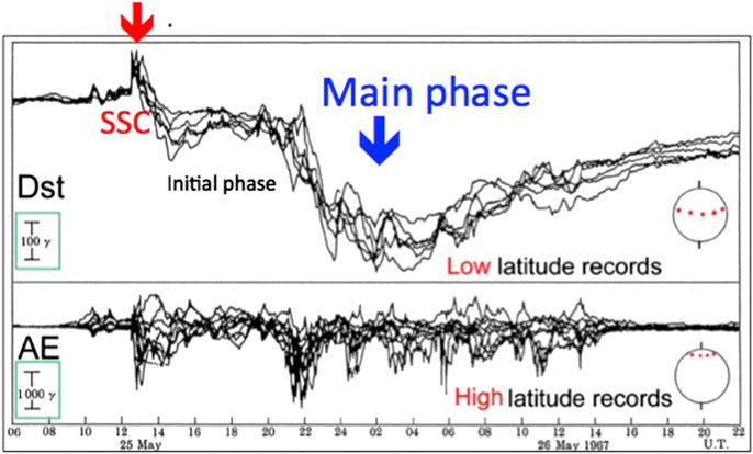
FIGURE 2. An example of the standard type of geomagnetic storms, indicating the ssc, initial phase, and the main phase. The upper part combines records from six stations in low latitude. Their average change is called the Dst index. The lower part combines records from 12 stations in high latitude; the upper envelop is called the AU index, the lower envelope the AL index, and (Au + AL) the AE index. Note the difference of the scale between low latitude and high latitude. Unit γ = nT.

Chapman worked at the Greenwich Observatory a little after Maunder and learned Maunder’s work. He decided to theorize Maunder’s finding, namely, how Maunder’s stream could cause geomagnetic storms. This work began with his graduate student Ferraro (Chapman and Ferraro, 1931).

Actually, Chapman had an earlier study on geomagnetic storms under the assumption of an electron beam, which was seriously criticized by Lindemann, who noted that an electron beam would disperse itself by its electrostatic force, but suggested the stream might consist of an equal number of protons and electrons, namely, the presently called “plasma”, in order avoid the dispersion.

The study by Chapman and Ferraro (1931) was basically on how a plasma stream interacts with a dipole magnetic field. They found that the Earth and its dipole field are enclosed in a comet-shaped cavity in the stream, Figure 3B. This comet-shaped structure is now called the magnetosphere; this term is coined by Gold (1959). When the steam arrives (or collides with a dipole field), the dipole field is “compressed” by the induced current at the front of the advancing plasma, resulting in the storm sudden commencement (ssc), Figure 3C. It is now considered that the ssc indicates the arrival of the shock wave which advances ahead of plasma clouds (CMEs).

FIGURE 3

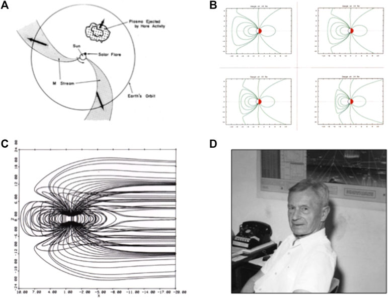
FIGURE 3. (A) The general view of interplanetary space until about 1958. (B) The compressed Earth’s dipole by a plasma flow from the Sun. (C) The compression of the front of the magnetosphere by an enhanced solar wind. (D) S. Chapman. Courtesy of the Geophysical Institute of the University of Alaska Fairbanks.

At that time, and until 1958, interplanetary space had been considered to be a vacuum, and only streams and gas clouds (CMEs) are intermittently emitted from the Sun (Figure 3A).

At the beginning of the last century, intense magnetic disturbances associated with intense auroral activities in the polar region got attention of our pioneers. This work began by Birkeland (1918). His electron beam from the Sun followed the magnetic field lines near the Earth (this beam current was much later called “Birkeland current”; this term is now used for field-aligned currents by some, but it is not correct, because field-aligned currents flow between the magnetosphere and the ionosphere, not from the Sun).

Independently, Chapman considered a current system on a spherical shell, which is called the “SD current” (Solar Daily magnetic disturbances, Figure 4B). The SD current became later the basis of the theories by Axford and Hines (1961) and Dungey (1961). Akasofu et al. (1965) showed that the main current has a single cell, Figure 4C.

FIGURE 4

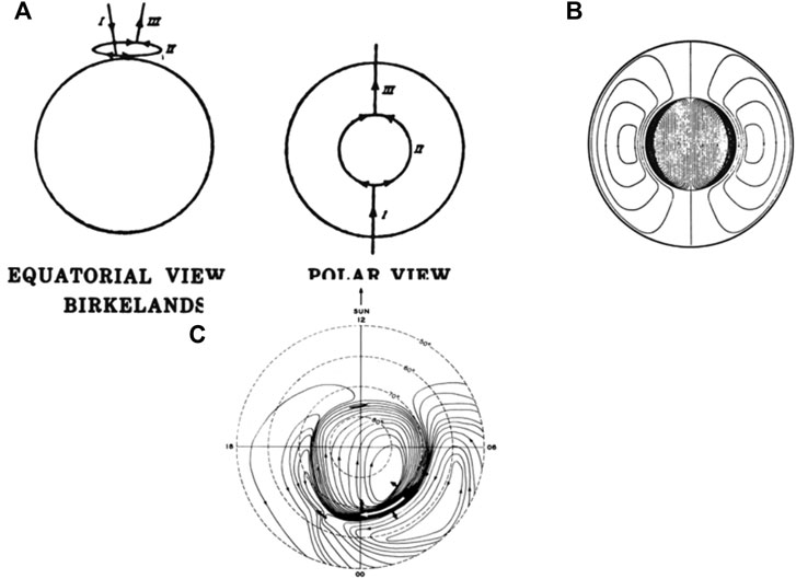
FIGURE 4. (A) Birkeland’s 3-D current system. (B) Chapman’s SD current. (C) The current proposed by Akasofu et al. (1965); note that the main current flows along the auroral oval, not along the auroral zone. Note also that unlike the two-cell SD current (B), it is a single cell current, as discussed in detail in The Unloading Current System.

As mentioned earlier, interplanetary space had long been considered to be a vacuum. Parker (1958) suggested that the solar corona blows out continuously and coined the term “solar wind”; he suggested also that the solar wind carries out the solar magnetic field in a spiral form. Thus, the magnetosphere is a permanent feature of Earth. Parker’s initial theory had been expanded by many others, but it was found later that it did not seem to work. On the other hand, there does not seem to be an acceptable theory on the origin of the solar wind at the present time; in fact, the satellite named “Parker” was recently launched to study the solar wind.

Early Studies (1960–1980)

The Interplanetary Magnetic Field

Since Chapman-Ferraro theory (1931) was published, there had been a large number of studies to find the way plasma particles enter into the magnetosphere to explain the main phase of geomagnetic storms and the aurora (or how protons in the solar wind enter the magnetosphere or how the solar wind energy is transmitted to the magnetosphere); as an example, the entry of solar plasma from the two neutral points on the front of the magnetopause (see Figure 3B) was once considered by many.

The nature of the interaction between the solar wind and the magnetosphere is one of the problems which has been seriously discussed until today. In this article, by taking the electric current approach, it is proposed that the interaction between the solar wind and the magnetosphere constitutes a dynamo, which supplies electric power (Poynting flux) for geomagnetic storms and auroras. The magnetic field line approach considers that this interaction causes the transfer of some of the day side magnetic field lines back to the magnetotail. It will be seen in Electric Current Approach; the dynamo approach is better in understanding subsequent processes in causing auroral substorms.

However, after the publication of the research by Chapman and Ferraro (1931) on the formation of the magnetosphere, no possible way for the particle entry was found until the 1960s. For example, I suggested once that one possibility for the entry of solar particles might be that the solar wind contains neutral hydrogen atoms, because they have no difficulty of crossing the magnetopause and could become ring current particles by exchanging the charge with terrestrial protons.

Since there was no simple way for the protons to enter or for the energy transfer at that time (except that Axford and Hines (1961) suggested a “viscous” interaction), I decided to reexamine Chapman’s definition of the standard geomagnetic storm (Figure 5). After examining a large number of geomagnetic storm records, it was found that geomagnetic storms develop in a great variety of ways, not necessarily in the standard way. In some cases, after a large ssc indicating the arrival of intense solar gas clouds, there occurs no main phase; such disturbances are thus not included in the list of geomagnetic storms (they are called a sudden impulse, si). In other extreme cases, an intense main phase occurs without ssc (without the impact of a strong solar wind (they are called gradually commencing storms, “sg”); such disturbances without ssc are also not listed as geomagnetic storms, because of no ssc); there are a variety of cases between the above two cases, Figure 5A.

FIGURE 5

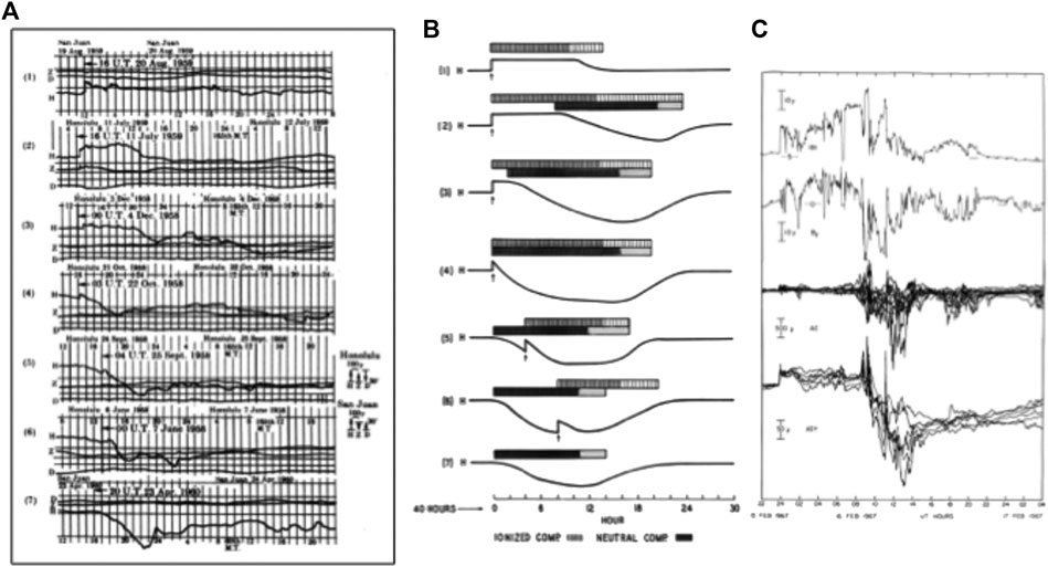
FIGURE 5. (A) It shows a number of ways of the development, indicating that geomagnetic storms do not necessarily develop in the standard way. (B) The figure suggests that the variety of the development is caused by different combination of pure plasma (white bar: protons and electrons) and the “unknown factor” (black bar: initially considered to be atomic hydrogen atoms). An example of geomagnetic storms with the IMF magnitude B and the Bz component: it shows clearly that the development of the main phase depends on the IMF Bz component.

Based on such a variety in the development of geomagnetic storms, I convinced Chapman that there must be some “unknown” factor in the solar wind or CMEs, which determines the development of the main phase (Akasofu and Chapman, 1963).

This consideration caused serious criticisms and controversies, because it was very firmly believed then that the solar wind (and clouds) consists of only protons and electrons. (Some of my colleagues said that I was not qualified as a graduate student, not knowing that the solar wind consists of protons and electrons.) However, Chapman became firm in believing that there must be “unknown” factor in the solar wind.

A little later, Dungey (1966) suggested that the “unknown” factor might be the southward component of the interplanetary magnetic field (Bz). Soon afterwards, Fairfield and Cahill (1966) showed that this is indeed the case. The “unknown” factor was found to be the IMF Bz.

The lesson here is that we have to be careful about the accepted “standard model” in natural phenomena; there may be a great variety of “exceptions” or “anomalies”, which may open a new idea or development.

After the solar wind data (n, p, V. B and IMF angle θ) became available, there were a large number of studies of the relationship between the solar wind parameters (and their combinations) and Kp, AE, and Dst; some of the early attempts are listed in Table 1 in Akasofu (1981).

I thought that it is better to examine the relationship between the solar wind and geomagnetic storms by considering that the solar-wind-magnetosphere interaction constitutes a dynamo and compare its power (erg/s or w) with the total dissipation rate UT (erg/s) or the total energy produced by the dynamo and total energy dissipation, Akasofu (1981).

The importance of the interplanetary magnetic field (IMF) became soon recognized in a number of observations. First of all, the magnetosphere is found to be an open system, not a closed system; solar subcosmic ray particles of less than 10 Mev (which cannot enter into the dipole field) were actually allowed to enter over the entire polar cap and the open system allows them to enter in the area encircled by the auroral oval. In the next section, it is shown that the “roots” of the open field lines (magnetospheric field lines which are linked with interplanetary magnetic field lines) are surrounded by the auroral oval (see Auroral Oval). This fact established the location of the auroral oval within the structure of the magnetosphere; note, however, that the exact location of open field boundary with respect to the poleward boundary of the oval is still uncertain.

Auroral Oval

It had long been believed for almost 100 years that the aurora is distributed along an annular belt, called “the auroral zone”, which is an annular belt centered at the geomagnetic pole (Loomis, 1860; Figure 6A). Feldstein (1963) found that the belt is considerably deformed from the annular belt and called it the auroral oval (Figure 6B); Loomis did not have auroral data in the highest latitude.

FIGURE 6

FIGURE 6. (A) Loomis' auroral zone. (B) Comparison of the auroral zone (pink) and Feldstein’s oval (green). (C) The comparison of the auroral oval and the intersection line between the outer boundary of the outer Van Allen belt, Akasofu (University of Iowa, Department of Physics Report). (D) The auroral oval and the “roots” of the linked field lines. (E) The distribution of the field-aligned current (Iijima et al., 1990).

However, his oval had not been easily accepted for a long time, because the auroral zone had been believed in for almost 100 years. In 1959, I made a number of visual auroral observations and noted the auroral distribution was somewhat different from Loomis’ auroral zone, because auroral arcs appear always from the northern sky and shift southward as the evening progresses. Thus, I supported Feldstein’s oval by setting up the Alaska meridian chain of all-sky cameras, which can “scan” the polar sky once a day (the largest scanning device on Earth); this was my first research supported by the National Science Foundation. However, this observation could not convince many of my colleagues.

Fortunately, it was found that the oval surrounds the “roots” of the linked magnetic field lines between IMF field lines and the magnetospheric field lines (Figure 6D). Further, it was found that the oval coincides with the intersection line between the ionosphere and the outer boundary of the outer Van Allen belt, Figure 6D. Furthermore, it was found that the distribution of field-aligned currents coincides also with the oval (Iijima et al., 1990, Figure 4.4E). These facts convinced our colleagues on the importance of the auroral oval; it was a sort of revolution in auroral studies, because the oval is the natural ordinate (not the auroral zone) in studying auroral phenomena.

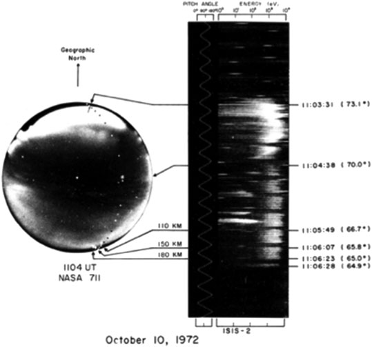
However, after all, the first image of the oval by satellite by Anger et al. (1972) was the most convincing of the presence of auroral oval.

One lesson I learned from this was that it is difficult to convince colleagues on a new morphological finding with additional morphological results alone; other almost unrelated observational results (such as Figures 6C,E, including satellite images) become more convincing in such cases.

The Main Phase and the Ring Current

Chapman and Ferraro tried to understand the cause of the main phase, although they could not find a way for solar wind protons to enter the magnetosphere. However, they thought that there must a westward current around Earth to explain the main phase (H component) decrease. They tried to examine only the stability of such a circular current round Earth, the ring current (Chapman and Ferraro, 1933).

When Van Allen and Frank (1959) reported the discovery of the Van Allen belts, Chapman thought that the belts were the ring current. Van Allen correctly identified that the particles in the belts execute motions, which correspond to one of the Stormer’s calculation of the orbit of charged particles trapped in a dipole field.

Chapman and Van Allen asked me to calculate the current in the belt and sent me to the Goddard Space Flight Center, NASA; there was an IBM 7090 for the Mercury Project (a super computer at that time). Akasofu and Chapman (1961) and Akasofu et al. (1961) found that for an isotropic pitch-angle distribution of protons, the current is basically the diamagnetic current, which consists of a weaker eastward current in the inner part of a belt, a stronger westward current in the outer part of the belt (Figure 7C). Thus, contrary to the general brief, the westward drift motion of positive particles does not contribute much to the westward current, although protons drift westward.

FIGURE 7

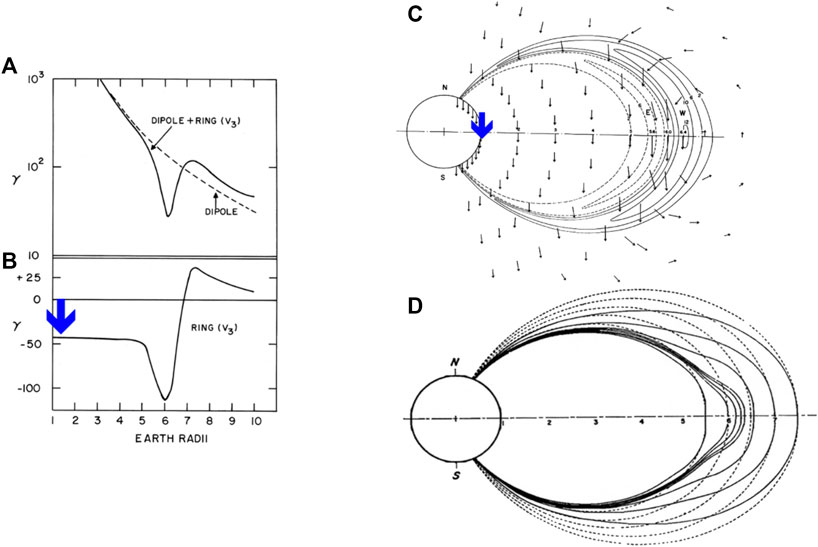
FIGURE 7. (A) The changes of the Earth’s dipole field produced by a model ring current. (B) The magnetic field produced by the ring current on the equatorial plane. The blue arrow indicates the main phase decrease. (C) The distribution of the current in the ring current and the magnetic field produced by the ring current. (D) The distortion of the Earth’s dipole field by the ring current.

This electric current study provided far more understanding of the ring current than magnetohydrodynamic approach discussed by Dessler et al. (1959), in which the ring current effects are expressed only by the total energy of the ring current particles. In fact, it is shown later that the acquired knowledge of the electric current here is crucial in understanding the cause of auroral/magnetospheric substorms and also the cause-effect relationship between the main phase of geomagnetic storms and substorms.

It was found also that the total energy of the Van Allen radiation belts cannot contribute much to the main phase, because the total energy is too small. Thus, it was considered that during geomagnetic storms, a new storm-time belt must be formed. Indeed, Frank (1970) reported such a storm-time proton belt during a geomagnetic storm.

Auroral Substorms

Morphology

It had long been thought that auroras were relatively quiet (quiet arcs, a curtain-shaped luminous structure) in evening hours, active in midnight hours (violent motions of arcs) and became patchy (disintegration of arcs, often referred to “break-up”) and that the Earth (and observers) rotated under such a sequence of the pattern once a night, observing the sequence of quiet to active to patchy auroras in one night. Thus, it was thought that auroral activities had a fixed pattern with respect to local time under which the Earth rotated once a day. This had been believed firmly for decades by most auroral researchers.

However, examining all-sky films from a few stations, I found that such a pattern (the sequence of quiet-active-patches) occurs often twice or thrice in one night. (Since the Earth does not rotate a few times a night) I decided to examine simultaneous Siberian (evening) and Canadian (morning) films, when auroras over Fairbanks (College) (midnight) became active on the basis of the IGY all-sky films.

I found that auroras repeat a fairly systematic activity over the whole polar region several times in 24 h (thus, a few times in one evening at a station). This particular auroral activity is called the auroral substorm (Akasofu, 1964); I sent my article first to Journal of Geophysical Research, but it was rejected. Thus, I sent it to Planetary Space Science (the editor then was D. R. Bates). It was the time when auroral research meant a study of auroral emissions (lines, bands), and all-sky cameras were not considered as a serious instrument, compared with sophisticated optical instruments.

The general acceptance of the concept of auroral substorms was not simple, because observers cannot stay in the midnight sector for at least 6 h to observe at least 2 auroral substorms. Both the NASA Galileo plane and the Air Force plane (KC 135) participated in this confirmation by flying westward from the East Coast to Alaska (constant local time flights). However, after all, a series of satellite images from a large distance above the polar region proved the concept of auroral substorms without doubt (Frank et al., 1982).

Auroral activities during substorms are complex, but there are a number of systematic activities, such as the poleward expansion in the midnight sector, westward traveling surges (WTS) in the evening sector, omega bands, and the so-called “patches” in the morning sector. Unfortunately, except WTSs, there have not been many studies of such individual activities, partly because the focus of research shifted to the cause of auroral substorms.

However, each display must tell differences of plasma conditions in the magnetosphere, which are definitely worth studying in order to understand magnetospheric conditions, in particular the asymmetry of auroral activities across the midnight meridian (Akasofu, 2012).

At about the same period, there had been a great variety of studies in high latitudes, including radio absorption (measured by riometers) and X-ray observations (by balloons), in addition to studies of auroras and geomagnetic disturbances. In the 1960s, a number of satellite observations joined in these studies and found that a number of disturbance phenomena in the magnetosphere occur simultaneously with auroral substorms.

Thus, it became obvious that both ground-based and satellite-based observations to be studied together in terms of a new term, magnetospheric substorms. This idea was proposed by N. Brice in 1967. The first compilation of all these observational studies was made by Akasofu (1967); the second summary was made also made by Akasofu (1977), assembling a large amount of ground-based studies and satellite studies; such data in the inner magnetosphere are still useful today, because the main effort of studying magnetospheric substorms after the 1970s has been focused mainly on the magnetotail.

Reasons for Objecting Against the Theory of Magnetic Reconnection

It has long been popular to consider that the magnetic energy is accumulated in the magnetotail and is released explosively by magnetic reconnection. This thought has been overwhelmingly popular in studies of auroral substorms.

Before discussing the electric current approach in the following, it is important to provide the reasons why I have strongly objected to such an idea, so that I do not refer much to magnetic reconnection in this review. It is hoped that there will be many reviews based on magnetic reconnection, so that the readers can compare both approaches.

(1) One of the strong reasons for that I have a strong objection on the concept of magnetic reconnection in as early as 1964 and still do is that any auroral activity associated with substorms proceeds outward (instead inward) soon after an arc brightens at the equatorward boundary of the auroral oval (not the poleward boundary) (Figure 9), namely an explosion, not an implosion.

FIGURE 9

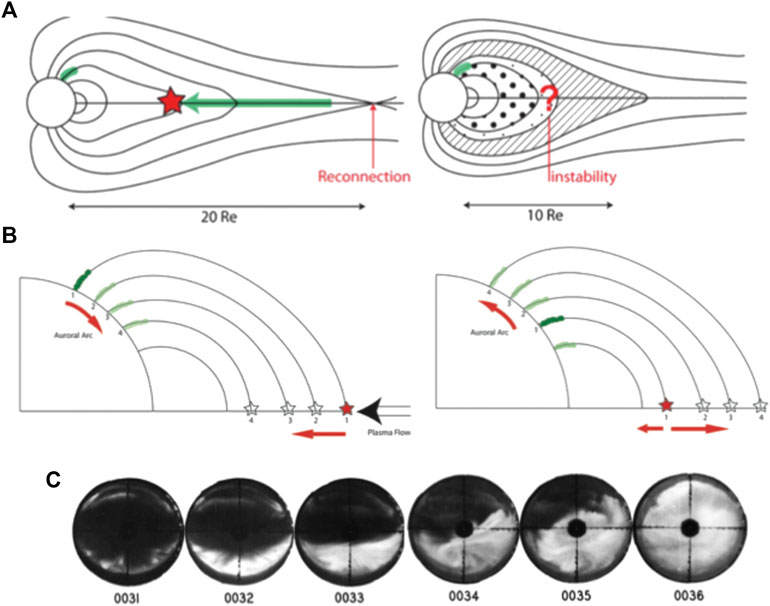
FIGURE 9. (A, B) Comparison of two ideas of the causes of the expansion phase, in which one considers that the source of auroral substorms is located in the magnetotail (magnetic reconnection) and its effect propagates inward, and the other considers an internal process (instability) in the inner magnetosphere. Magnetic reconnection suggests that auroral activities propagate inward, while a process of internal origin propagates outward. (C) An example of all-sky images of the outward propagation of auroral activities after the initial brightening.

FIGURE 8

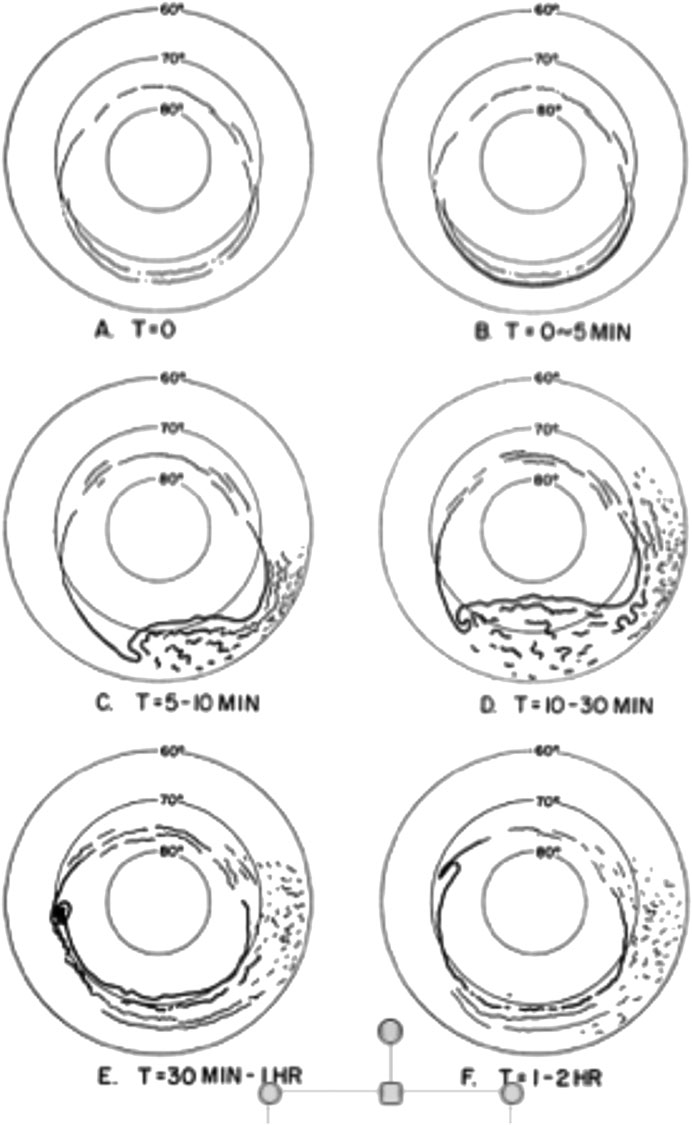
FIGURE 8. A schematic representation of auroral activities during the expansion phase of auroral substorms (Akasofu, 1964).

There is no prominent auroral activity poleward of the arc which brightens first at the onset of the expansion phase, suggesting that the onset is a process which begins deep inside the magnetosphere, instead of outside triggering of the onset (the initial brightening of an arc); if the energy would come from the magnetotail, there would be some specific auroral activity poleward of the arc prior to the onset, but no such activity is seen in all-sky cameras and satellite images in the midnight sector.

(2) Another strong reason for which I oppose magnetic reconnection in the magnetotail as the energy source of substorms is that the location of the initial brightening arc is at the southward boundary of the auroral oval (not the northern boundary), which coincides with the outward boundary of the trapping region, which is located at a distance of about 5–6 Re (Re = the Earth’s radius); see Appendix. The latitude of the initial brightening arc can occur at latitude below 50° during intense geomagnetic storm, and corresponding L can be 2.4, although the ring current can change it to perhaps to L = 4. This is an important fact in considering the location of the initial brightening of an auroral arc at the onset of the expansion phase of auroral substorms.

These are the simplest observational facts that anyone can understand. The problem is that once a theoretical idea, such as magnetic reconnection, becomes overwhelmingly popular, observational facts which contradict with it tend to be dismissed or ignored.

Electric Current Approach

In this section, we introduce the electric current approach in studying specifically auroral substorms. Alfven (1967) proposed the electric current approach by stating: “in many cases the physical basis of the phenomena is better understood if the discussion is centered around the picture of the current lines (rather than the magnetic field line approach)”.

In the electric current approach, we consider that natural electromagnetic phenomena are caused by a chain of processes, consisting of power supply (dynamo), transmission (currents/circuits), and dissipation (most of observed phenomena, such as auroral substorms and solar flares); Figure 10.

FIGURE 10

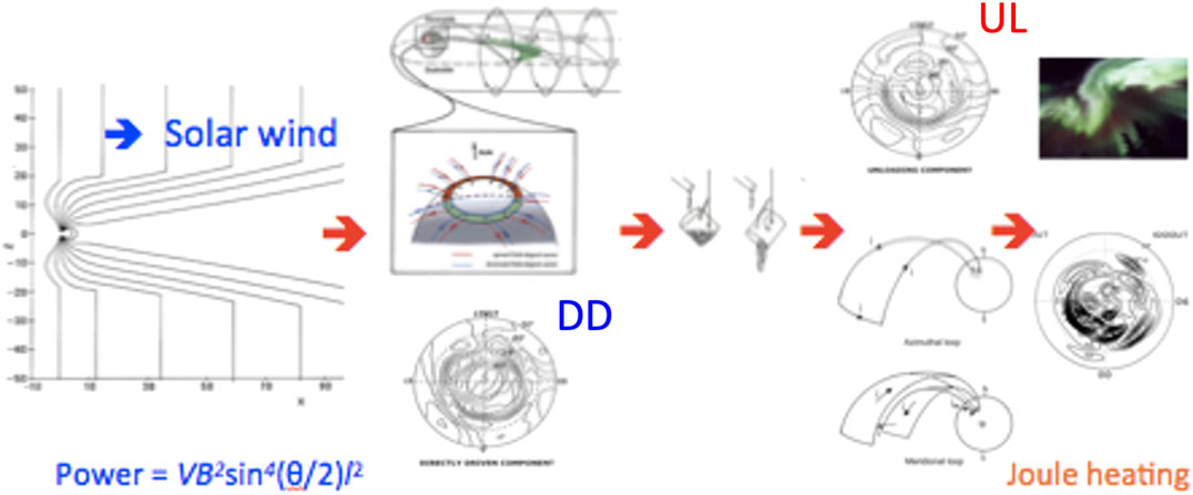
FIGURE 10. The auroral substorm processes, starting from the solar-wind-magnetosphere dynamo, the magnetospheric current circuit, the accumulation-release (unloading) process, the circuit of the expansion phase, and the resulting ionospheric Joule heating (dissipation).

Actually, this is supposed to be the basic approach in considering any electromagnetic phenomena. Taking this approach, we have begun to understand why and how the growth phase occurs, where the energy for the expansion phase is accumulated and released and how the earthward electric field for Bostrom’s current system (Bostrom, 1964) may be set up. However, it should be emphasized that what is presented here is still in a rudimental stage (Akasofu, 2017).

Figure 10 shows the chain of processes in a concrete way for auroral substorms, from the dynamo process to the ionospheric dissipation. We begin with the first process, the dynamo process quantitatively as the power supply for auroral substorms. (In the magnetic field line approach, the power supply process is considered as the field line transfer from the dayside to the night side.)

The dynamo process occurs as a result of the interaction between the solar wind and the Earth’s magnetic field. The power is generated by the fact that the solar wind of speed (V) flows across the linked magnetic field (B) between the interplanetary (solar) magnetic field (IMF) and the magnetic field of the magnetosphere (Akasofu, 2017), Figure 10.

The power of the solar-wind-magnetosphere dynamo is defined by the Poynting flux p (erg/s or w):

$P=\text{ ∫}\left(E\text{ × }B\right)•\mathrm{ds}=V(B^{\text{2}}/\text{8π})S\text{.}$

Typical values of the parameters are as follows:

Solar wind speed V = 500 km/s,

$\text{IMF }B=10\text{ nT,}$

S = sin⁴ (θ/2) (l²π), l = 10 Re, (Re = the Earth’s radius), θ = the polar angle of the IMF (the angle θ = 180° indicates the IMF is oriented southward),

$P=2\text{.0 x}{10}^{19}\text{ erg}/\text{s}\left(2\text{.0x}{10}^{12}\text{ w}\right).$

The power generated by the dynamo flows in the direction of E x B. Thus, in a dipolar configuration, much of the power is directed toward the inner magnetosphere (Figure 11A). The increased power produced by the dynamo manifests itself as an increased magnetospheric current in the inner magnetosphere, much more than in the magnetotail (Figure 11B).

FIGURE 11

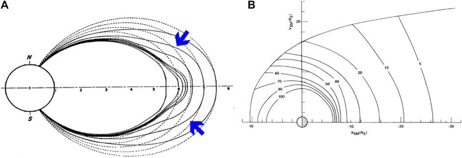
FIGURE 11. (A) The figure shows the direction of the flow of power generated by the solar-wind-magnetosphere dynamo and resulting inflation of the magnetosphere. (B) The magnetospheric current on the equatorial plane (Olson, 1984).

Substorm-Associated Magnetic Disturbances and Current Systems

In the electric current approach, it is essential to have an accurate knowledge of electric currents around the Earth. The only way we can monitor changes of the currents continuously at fixed points for an extended period in magnetospheric physics is ground-based magnetometer observations.

Ground-Based Observations

Since ground-based magnetic field observations and the resulting knowledge of electric currents play a crucial role in substorm studies, this section is devoted to this study. In fact, it is this study by which the electric current approach has made an important progress in substorm studies. As mentioned earlier and in Figure 4, geomagnetic disturbances in high latitudes had been a long-studied subject, and various current systems had been proposed. Although these disturbances occur during auroral activities, the two subjects had been almost independently pursued until about 1960, partly because of lack of simultaneous data sets.

When the concept of auroral substorms was introduced, it was recognized that both subjects should be studied together. Both phenomena are caused by electric currents in the upper atmosphere; electrons carrying the current collide with upper atmospheric atoms and molecular, which emit auroral lights, while the currents produce magnetic fields, which we observed as magnetic disturbances. Thus, both auroral activities and geomagnetic disturbances result from the electric currents.

In the 1970s, it became urgent to upgrade the distribution of magnetic observatories. By an international effort, six meridian chains of the observatories were established in the 1970s, enabling us to determine fairly accurately the distribution of currents in the polar ionosphere with a time resolution of 5 min (Figure 12).

FIGURE 12

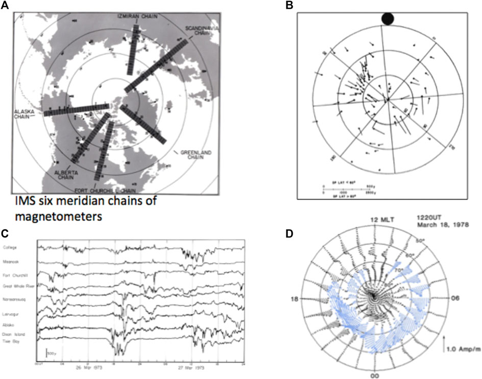
FIGURE 12. (A) The location of the six meridian magnetic stations. (B) An example of magnetic records (the H component) from a number of arctic stations. (C) An example of the distribution of disturbance vectors determined from the H and D components. (D) An example of electric current vectors; a special computer code was developed by Kamide et al. (1982) to convert the magnetic disturbance vectors into the current vectors.

Figure 13 shows an example of the growth and decay of the polar current during the expansion phase. The current system during the expansion phase was extensively analyzed later. This was an extremely laborious task and had taken 2 decades or so. Alfven used to complain of the slow progress to me, saying “too slow, too slow”.

FIGURE 13

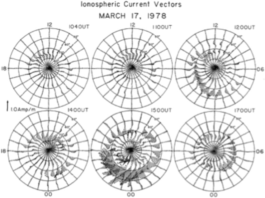
FIGURE 13. An example of the growth and decay of electric currents during the expansion phase of auroral substorms.

In fact, the current distribution and its time variations thus obtained have advanced the electric current approach in substorm studies. The results are described in The Roles of the Magnetosphere.

Controversy on the Current System

In order to explain the strong westward current in Figure 13, called the auroral electrojet, there have been two models, one is proposed by Bostrom (1964) and the other is called the “current wedge” model (McPherron et al., 1983).

There has been a considerable discussion on both current systems. The current wedge model suggests that the cross-tail current is diverted to the ionosphere. Since this model assumes basically a short circuiting of the cross-tail current, the electrojet current must be basically the Pedersen current driven by a westward electric field.

Various electric field observations by incoherent scatter radars (Brekke et al., 1974) and the superDarn observations (Bristow and Jensen, 2007) indicate that the electric field driving the electrojet is directed southward (equatorward, not westward), indicating that the jet current is the Hall current, which flows in the direction perpendicular to the electric field. Further, in the current wedge model, it is not clear why the cross-tail current has to be diverted to the resistive ionosphere. (I considered once the current wedge model but gave it up by realizing the nature of the current.)

The other possibility is a 3-D current system proposed by Bostrom (1964), which will be discussed later in detail (Figure 16A). In fact, it will be shown that this current system can quantitatively explain various observed features of the expansion phase, although much more studies are needed to find an accurate current system for the expansion phase. It is hoped that better current systems will be proposed by a new generation in the future.

One of the important facts in choosing a possible current system is that it has to explain the arc structure. An auroral arc is a curtain of light; its width is less than 1 km, although satellite observations show a little wider structure (the “inverted V” structure). Thus, an electron beam has to have a sheet form, although it is not yet known why the field-aligned current forms a thin sheet current (often multiple). The meridional component of Bostrom’s model has a sheet current structure, while the current wedge model would produce a bright spot only at the western edge of the electrojet, where there is an upward current. For these reasons, we consider only Bostrom’s 3-D current system in the following sections.

The Roles of the Magnetosphere

The Basic Concept of the Energy Accumulation

In order to explain the explosive feature of auroral activities, its energy must be stored once before the expansion phase.

It was considered in early days that changes of auroral activities were simply proportional to changes of the intensity of the solar wind as a function of time, in which the dissipation follows closely varying solar wind intensity (power).

However, the sudden onset and the subsequent rapid poleward motion of arcs during the expansion phase is explosive, suggesting that solar wind energy may be accumulated once before the onset of the expansion phase and then suddenly releasing a tippy pitcher model (Figure 14), in which the dissipation does not follow changes of the power. After much discussion, these two ideas were eventually combined (Rostoker et al., 1972) by recognizing that the magnetosphere has both capabilities.

FIGURE 14

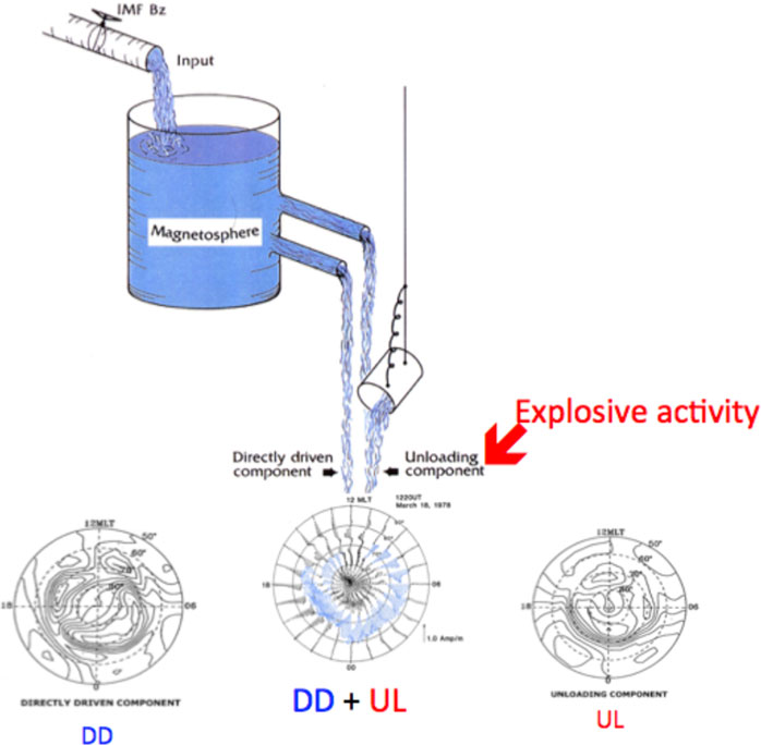
FIGURE 14. The tank-tippy pitcher model. What we can observe by a ground-based magnetometer network is (DD + UL). The figure shows also both the DD and UL components.

Thus, it became necessary to identify the two components in the currents, namely, the directly driven (DD) component and the unloading (UL) component (the explosive component). Both components can best be monitored by the ionospheric current. However, what we observe by the ground-based magnetometer network is (DD + UL). Thus, in order to study the expansion phase, it became necessary to separate the DD and UL currents (Sun et al., 2000).

DD Current

It was found that the DD current is found to be a two eddy current, namely, a two-cell current in the polar ionosphere (Figure 14), which is the ionospheric manifestation of plasma convection (Figure 15A) and also which has driven the electric field across the magnetosphere (directed from the morning side to the evening side), Axford and Hines (1961). This magnetospheric convection induces the ionospheric convection, but in the lower ionosphere (the E-layer) electrons carry the current, because ions become immobile by the neutral particles. The electrons flow along the convection contours, but in the direction opposite to the convection. Actually, it is an improved version of Chapman’s SD current (Figure 15D) and is greatly distorted by the anisotropic conductivity of the ionosphere.

FIGURE 15

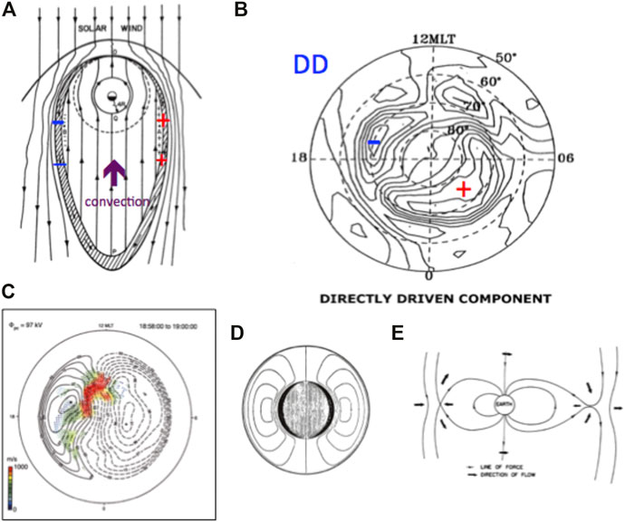
FIGURE 15. (A) The convection pattern of plasmas in the equatorial plane, suggested by Axford and Hines (1961) on the basis of Chapman’s SD current. (B) The ionosphere convection pattern (the same as the DD current; the current line is the same as the convection line) based on the analysis of the six meridian chains of station. (C) An example of the superDarn observation of the ionospheric convection. (D) Chapman’s SD current. (E) Dungey of convection model based on the SD current.

FIGURE 16

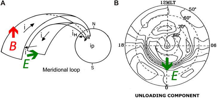
FIGURE 16. (A) Bostrom’s 3-D current system for the expansion phase. (B) The UL current in the ionosphere deduced on the basis of the six meridian chains of magnetometers. The earthward electric field becomes a southward (equatorward) electric field E.

The current pattern is confirmed by the superDarn observation (Bristow and Jensen, 2007), which observes the convection pattern of plasma in the ionosphere; compare Figures 15B,C. It may be noted that in his 1961 paper, Dungey attempted to explain the SD current by a convective motion of magnetic field lines (Figure 15E).

The UL Current System

The UL current system occurs impulsively during the expansion phase. The UL current system is a sheet current, of current density of more than 10 μmA/m², which can explain curtain-like structure of auroral arcs. In the ionosphere, it is a single cell current, as shown in Figure 16; its early version is shown in Figure 4C. Figure 16C provides an accurate version of the UL current in the ionosphere, the auroral electrojet. The UL current is the ionospheric part of the current system proposed by Bostrom (1964), which is shown in Figure 16A.

This current system can be driven by an earthward electric field on the equatorial plane; in the circuit, the condition of J • E < 0 is present only on the equatorial plane, so that the electric field driving the current system must be there. This electric field is one of the most crucial facts in determining the expansion process. The major phenomena associated with the expansion phase can be caused by this UL 3-D current system, as shown in the following. It should be reminded that it is crucial to determine an accurate current system, either improving Bostrom’s current system or a better one.

Joule Heating Dissipation

In any study of natural electromagnetic phenomena, the amount of dissipation is one of the major subjects. In auroral/magnetospheric substorms, the main dissipation occurs as the Joule heating in the ionosphere. Thus, it is crucial to study the Joule heating on the basis of the distribution of the ionospheric current, Figure 17; note that 1 mW/m² = 1 erg/cm²s (Ahn et al., 1983).

FIGURE 17

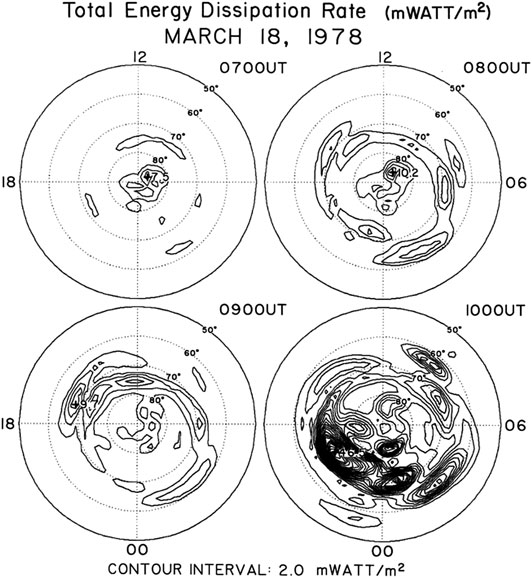
FIGURE 17. The development of the Joule heat dissipation rate during a substorm (Ahn et al., 1983).

The Joule heat production rate is proportional to the ionospheric current intensity. The Joule heat production is the main dissipation process for substorms and is proportional to the current intensity I in the ionosphere {the Joule heat production rate δ [= I²/σ= (I/σ)I ∞ I]}; this is because the field-aligned currents (connected to the UL field-aligned currents) produce the ionization in the ionosphere; σ denotes the conductivity of the ionosphere.

Actually, until Ahn et al. (1983) estimated the amount of the joule heat dissipation and its rate (Figure 10), there was no definitive estimate of the energy consumed by a substorm and its rate; all theoretical studies of magnetic reconnection before 1986 had been made without knowing accurately the amount of the output and its rate.

Directly Driven and Unloading Currents

The roles of the directly driven (DD) current and the unloading (UL) current on substorm processes can be examined by their time variations.

Fortunately, as mentioned earlier, the current intensity is roughly proportional to the Joule heating dissipation rate, because as explained earlier, the ionospheric conductivity is proportional to the current intensity.

Figure 18A shows how the DD and UL currents vary during the growth, expansion, and recovery phases.

(1) The DD current begins to grow during the growth phase.

(2) The UL current grows significantly later (about one hour), but it is short lived.

(3) The DD current remains strong even after the expansion phase.

FIGURE 18

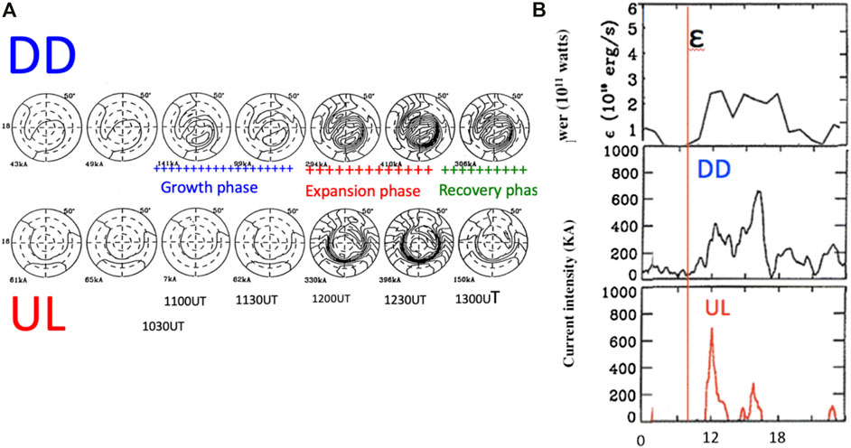
FIGURE 18. (A) Changes of the directly driven (DD) current and the unloading (UL) current during a typical substorm; the three phases are shown. (B) The relationship between the power P (= ε /8π), the intensity of the DD current, and the UL current during the same substorm as Figure 12A. The red line is a guide to show the relative time relationship between the three quantities. Both are for the same substorm.

In Figure 18B, we examine the above relationship more quantitatively as a function of time. One can see more clearly the above changes of the DD and UL currents in association with the power generated by the dynamo:

(1) The DD current follows fairly well the power P (= ε/8π).

(2) The DD current grows more slowly than the power at the beginning.

(3) The onset of the UL current begins after a significant delay of about one hour behind the DD current. This delay period is called the growth phase.

(4) The above facts indicate that the power is not dissipated much during the growth phase and thus must be accumulated in the inductive circuit of the magnetosphere.

(5) Unlike the DD current, the UL current occurs impulsively (unrelated to time variations of the power P).

(6) The main UL current occurs only during an early epoch of substorms (despite the fact that the power is maintained high even after the end of the expansion phase).

(7) The above fact indicates that there is no large accumulation of the power after the ionosphere becomes ionized enough to conduct the current (producing enough the Joule heat and thus dissipating the power), indicating that there is no accumulation after the expansion phase and that the accumulated energy is totally unloaded.

(8) The DD current is enhanced during and after the expansion phase and lasts until the power becomes less than 10¹¹ w.

As mentioned earlier, the power generated by the dynamo flows in the direction of the Poynting flux (ExB). Thus, in the magnetosphere, the flux tends to be directed mainly toward the inner magnetosphere (because of a dipolar configuration), Figure 11A. As a result, the inner magnetosphere becomes “inflated” by the accumulating power. The accumulation of the power is manifested by an increase of the current across the magnetosphere or the resulting changes of the magnetic field configuration at about the distance of 6 Re for medium intensity substorms, Figure 11B.

Cause of Auroral Substorms

Inflation and Deflation

As a result of the increasing current at about 6 Re, the magnetosphere becomes inflated during the growth phase (Figure 19A, blue arrow); the inflation can be observed by calculating the resulting deformation of the magnetic field configuration, as shown in Figures 7D, 19A; these show the results for the loaded energy of 3 × 10²¹ erg/s around 6 Re, which is a little less than the amount in making the magnetosphere unstable. Lui (2020) considered a specific current instability for this cause.

FIGURE 19

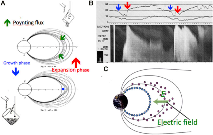
FIGURE 19. (A) The inflation-deflation sequence. (B) The inflation (blue arrow)-deflation (red arrow) sequence is observed as a sequence of decrease-increase of the magnetic field intensity at 6 Re (DeForest and McIlwain, 1971), together with a sudden increase of the electron flux at the time of deflation. (C) During the deflation, electrons are closely tied to inward moving magnetic field lines, while protons are not. Thus, a charge separation is expected to occur during the deflation, generating an earthward electric field, which can drive Bostrom’s current system during the expansion phase.

When the current across the equator and thus the magnetosphere become unstable, the accumulated energy will be unloaded (UL), and thus the magnetosphere is deflated, Figure 19A (red arrow). The nature of the current instability has recently been investigated (Lui, 2020).

When the current is reduced and the energy is unloaded (released), the magnetosphere is “deflated”. An observational example of both the inflation and deflation (causing a decrease and the subsequent increase of the magnetic field intensity) will be discussed in the following.

In the magnetic field observation around 6 Re, we can see a sequence of the inflation (blue arrow) and deflation (red arrow). In Figure 19B, when the inflation occurs, the magnetic field intensity is decreased (blue arrow) inside the enhanced current (Figure 11B), while a sudden deflation is manifested by a sudden increase of the field intensity (red arrow, Figure 19B), accompanied by a sudden increase of the electron flux, Deforest and McIlwain (1971).

During the deflation, a charge separation is expected to occur, because electrons are tightly bound to the contracting field lines where the deflation occurs, while protons may not (Lui and Kamide, 2003). The electrons attached to the contracting field lines will be discharged, causing the sudden brightening of an arc, substorm onset; note that the locations of the initial brightening arc and the corresponding L value are naturally determined by understanding the location the accumulated energy is at about 6 Re for medium intensity substorm. Figure 19C shows schematically how the charge separation could cause the earthward electric field. The expected electric field E is given by one of the Maxwell’s equations, E = [−(∂Bz/∂t)∫∂y]≈ 5–50 mV/m. Note that J•E < 0 occurs only in the equatorial part of the circuit of Bostrom’s current system (Figure 16A).

Fortunately, there is a very important set of observations at 8.1 Re (in the inner magnetosphere), showing a sequence of events, leading to the deflation at the time of a substorm onset (Lui, 2011) and the simultaneous occurrence of the following:

(1) a rapid reduction of the current,

(2) breakdown of the frozen-in field condition,

(3) occurrence of the earthward electric field.

The breakdown of the frozen-in-field condition is crucial for the suggested charge separation, resulting in the earthward-oriented electric field (it is unlikely that in any theory, the expansion phase cannot be explained if the frozen-in field condition is assumed. In turn, the resulting electric field drives Bostrom’s 3-D current system [the UL current system]), (Figure 16A). This observation suggests that the current instability seems to develop rather suddenly.

Cause of Auroral Substorms

Substorms occur when the power is typically 3–5 × 10¹⁸ erg/s or 3–5 × 10¹¹w, so that the accumulated energy W during the growth phase (about 1 h) becomes about 5 × 10²² erg (or 5 × 10¹⁵ J). This is about the energy dissipated during a substorm, as we observed in DD and UL currents and cause of auroral substorms.

Thus, the power accumulated during the growth phase is almost totally dissipated during the expansion phase (the energy accumulated in the tippy pitcher is emptied in each substorm). Note that W = (1/2) I² L = 5 × 10²² erg for about L = 100 H, I = 10⁷ A (cf. Alfven, 1981).

This is one of the possible scenarios to explain the expansion phase of auroral substorms on the basis of the electric current approach. Since this approach has just been initiated, the sequence of the processes should be more carefully investigated.

In fact, different sequences based on the facts obtained by the analysis of the DD and UL currents or even on the basis of a different set of observations are most welcome. For this purpose, in the future, satellite observations within 10 Re are needed, rather than in the magnetotail.

It is quite likely that other scenarios can be set up on the basis of some of the observed facts and results mentioned in the above. Indeed, this is the most challenging problem. Thus, it can be stated that a new study of auroral/magnetospheric substorms has just begun. The two things quite certain in this chain of thought are Bostrom’s 3-D current system and the earthward electric field which generates it.

We have considered so far the enhanced current located around 6 Re for medium intensity substorms. Several other observations suggest that the location of the power accumulation varies, depending on the intensity of substorms, 4 Re for most intense substorms (AE index 2000 nT) and 10 Re for weakest substorms (AE index 100 nT), Akasofu, 2017).

The Poleward Expansion

One of the most prominent auroral activities during substorms is the poleward expansion, as the name expansion phase indicates, Figure 20. For moderate substorms, the speed of the poleward advance of arcs is about 250 m/s; during a very large substorm, both the speed and the extent of advance can be several times greater.

FIGURE 20

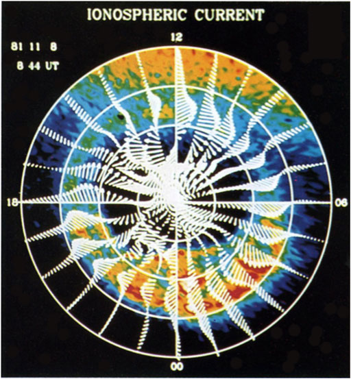
FIGURE 20. An example of simultaneous observation of the aurora by a satellite and the distribution of electric currents obtained by the six meridian chains of magnetometers (Electric Current Approach), Craven et al. (1884).

Figure 20 shows an example of the simultaneous observation of the aurora and the electric current in the ionosphere for intense substorms. One can see in this case that both the aurora and the electrojet reached as far as 78° in latitude. The magnetic field produced by the 3-D UL current system (B, red arrow in Figure 16A) shifts the earthward end of the azimuthal component poleward, causing the poleward advance of arcs and the auroral electrojet; for a typical value B = 50 nT (moderate substorms), it can shift the end of the azimuthal component about 500 km (corresponding to about 5° in latitude) as often observed.

Conclusion

There are a large number of fundamental unsolved problems in space physics, because we have to start a new study of auroral substorms, emphasizing the electric current approach. However, the electric current approach is “new” in space physics, so that it is still in a very rudimental stage. Thus, new generations of researchers are most welcome in pursuing the electric current approach. This approach is more instructive, because we can learn the physics involved deeper than the magnetic field line approach.

Author Contributions

The author confirms being the sole contributor of this work and has approved it for publication.

Conflict of Interest

The author declares that the research was conducted in the absence of any commercial or financial relationships that could be construed as a potential conflict of interest.

Acknowledgments

We owe many pioneers, senior researchers, and colleagues in bringing space physics this far, especially Sydney Chapman and Hannes Alfven. I myself owe many colleagues in reaching this far, in particular those who worked with me in developing the electric current approach, C. I. Meng, Y. Kamide, Sun Wei, and B. H. Ahn. I would like to thank all space physicists at this occasion of completing the present work. I would like to thank specially A. T. Y. Lui who has worked closely with me from the earliest days in space physics and who invited me to joint this special issue.

Appendix

In order to confirm the location of the discrete aurora and the diffuse aurora (caused by the outer belt), there has been a simultaneous observation of the auroras along a trajectory of a satellite. All-sky image shows both active auroras to the north and the diffuse aurora to the south (caused by the trapped particles).

References

Ahn, B.-H., Akasofu, S.-I., and Kamide, Y. (1983). The Joule heat production rate and the particle injection rate as a function of the geomagnetic indices AE and AL. J. Geophys. Res. 88, 6275–6287. doi:10.1029/JA088iA08p06275

CrossRef Full Text | Google Scholar

Akasofu, S.- I. (1964). The development of the auroral substorm. Planet. Space Sci. 12, 273–282. doi:10.1016/0032-0633(64)90151-5

CrossRef Full Text | Google Scholar

Akasofu, S.-I. (2017). Auroral substorms: search for processes causing the expansion phase in terms of the electric current approach. Space Sci. Rev. 212, 341–381. doi:10.1007/s11214-017-0363-7

CrossRef Full Text | Google Scholar

Akasofu, S.-I., Chapman, S., and Meng, C.-I. (1965). The polar electrojet. J. Atmos. Terr. Phys. 27, 1301–1305. doi:10.1016/0021-9169(65)90087-5

CrossRef Full Text | Google Scholar

Akasofu, S.-I., and Chapman, S. (1963). The development of the main phase of magnetic storms. J. Geophys. Res. 68, 125–129. doi:10.1029/JZ068i001p00125

CrossRef Full Text | Google Scholar

Akasofu, S.-I., and Chapman, S. (1961). The ring current geomagnetic disturbance, and the Van Allen radiation belt. J. Geophys. Res. 66, 1321–1350. doi:10.1029/JZ066i005p01321

CrossRef Full Text | Google Scholar

Akasofu, S-I. (1981). Energy coupling between the solar wind and the magnetosphere. Space Sci. Rev. 28, 121–190. doi:10.1007/BF00218810

CrossRef Full Text | Google Scholar

Akasofu, S.-I. (1977). Physics of magnetospheric substorms. Dordrecht-Holland: D. Reidel Publication Co.

Google Scholar

Akasofu, S.-I. (1967). Polar and magnetospheric substorms. Dordrecht-Holland: D. Reidel Publication Co.

Google Scholar

Akasofu, S.-I. (2012). “The morphology of auroral substorms,” in Auroral phenomenology and magnetospheric processes. Editor A. Keiling, E. Donovan, F. Bagenal, and T. Karlsson (AGU Monograph), Vol. 197.

Google Scholar

Akasofu, S. –I., Cain, J. C., and Chapman, S. (1961). The magnetic field of a model radiation belt, numerically computed. J. Gephys. Res. 66, 4013–4026. doi:10.1029/JZ066i012p04013

CrossRef Full Text | Google Scholar

Alfven, H. (1981). Cosmic plasma. Dordrecht-Holland: D. Reidel Publication Co.

Google Scholar

Alfven, H. (1967). “The second approach to cosmical electrodynamics,” in The Birkeland symposium on aurora and magetic storms. Editors A. Egeland, and J. Holtet (Paris, France: Centre National de la Rescherche), 439–444.

Google Scholar

Anger, C. D., Lui, A. T. Y., and Akasofu, S.-I. (1972). Observations of the auroral oval and a westward travelling surge from the ISIS-2 satellite and Alaskanm meridian chain all-sky camera. J. Geophys. Res. 78 (16), 3020–3026. doi:10.1029/JA078i016p03020

CrossRef Full Text | Google Scholar

Axford, W. I., and Hines, C. O. (1961). A unifining theory of high-latitude geophysical phenomena and geomagnetic storms. Can. J. Phys. 39, 1433–1464. doi:10.1029/GM018p0936

CrossRef Full Text | Google Scholar

Birkeland, K. R. (1918). The Norwegian auroral Polaris Expedition. 1902–1903.

Google Scholar

Bostrom, R. (1964). A model of the auroral electrojet. J. Geophys. Res. 69, 4983–4999.

Google Scholar

Brekke, A., Doupnik, J. R., and Banks, P. M. (1974). Incoherent scatter measurements of E region condictivities and currents in the auroral zone. J. Geophys. Res. 79, 3773. doi:10.1029/JA079i025p03773

CrossRef Full Text | Google Scholar

Bristow, W. A., and Jensen, P. (2007). A superposed epoch study of superDarn convection observations during substorms. J. Geophys. Res. 69, 112. doi:10. 1029/2006JA012049

CrossRef Full Text | Google Scholar

Chapman, S. (1918). An outline of a theory of magnetic storms. Proc. Royal Soc. 97, 61–83. doi:10.1098/rspa.1918.0049

CrossRef Full Text | Google Scholar

Chapman, S., and Ferraro, V. C. A. (1931). A new theory of magnetic storms. Terr. Mag.Atmos. Elect. 40 (4), 349–370.

Google Scholar

Chapman, S., and Ferraro, V. C. A. (1933). A new theory of magnetic storms. Terr. Mag. Atmos. Elect. 38 (2), 79–96. doi:10.1029/TE38002p00079

CrossRef Full Text | Google Scholar

Craven, J. D., Kamide, Y., Frank, L. A., Akasofu, S.-I., and Sugiura, M. (1884). “Distribution of aurora and ionospheric currents observed simultaneously on a global scale,” in Magnetospheric currents (Washingon, DC: AGU), 28, 137–146.

Google Scholar

Deforest, S. E., and McIlwain, C. E. (1971). Plasma clouds in the magnetosphere. J. Geophys. Res. 76, 3587–3611. doi:10.1029/JA076i016p03587

CrossRef Full Text | Google Scholar

Dessler, A. J., and Parker, E. N. (1959). Hydromagnetic theory of geomagnetic storms. J. Geophys. Res. 64, 2239–2252. doi:10.1029/JZ064i012p02239

CrossRef Full Text | Google Scholar

Dungey, J. W. (1961). Interplanetary magnetic field and the auroral zones. Phys. Rev. Lett. 6 (20), 47–48. doi:10.1103/Phys.RevLett.6.47

CrossRef Full Text | Google Scholar

Dungey, J. W. (1966). “Solar-wind interaction with the magnetosphere.Particle aspects,” in The Solar wind. Editors R. J. Mackinjr., and M. Neugebauer (Pasadena, California: Jet Propulsion Laboratory), 243–255.

Google Scholar

Fairfield, D. H., and Cahill, L. J. (1966). Transition region magnetic field and polar magnetic disturbances. J. Geophys. Res. 71 (1), 155–169. doi:10.1029/JZ071i00155

CrossRef Full Text | Google Scholar

Feldstein, Y. I. (1963). Some problems concerning the morphology of auroras and magnetic disturbances at high latitudes. Geomagn. Aeron. 3, 183–192.

Google Scholar

Frank, L. A., Craven, J. J., Burch, J. L., and Winninham, D. J. (1982). Polar view of the earth with dynamic explorer. Geophys. Res. Lett. 9 (9), 1001–1004. doi:10.1029/GL009i009p01001

CrossRef Full Text | Google Scholar

Frank, L. A. (1970). Direct observation of asymmetric increase of exstraterresstrial ‘ring current’ proton intensities in the outer radiation zone. J. Geophys. Res. 75, 1268. doi:10.1029/JA075i007p01263

CrossRef Full Text | Google Scholar

Gold, T. (1959). Motions in the magnetsosphere of the earth. J. Geophys. Res. 64 (9), 1219–1224. doi:10.1029/JZ064i009p01219

CrossRef Full Text | Google Scholar

Iijima, T. T. A., Potemura, , and Zanetti, L. J. (1990). Large-scale characeristics of magnetospheric equatrial currents. J. Geophys. Res. 95, 991–999. doi:10.1029/JA095iA02p00991

CrossRef Full Text | Google Scholar

Kamide, Y., Ahn, B.-H., Akasofu, S.-I., Baumjohann, W., Friis-Christensen, E., Kroehl, H. W., et al. (1982). Global distribution of ionospheric and field-aligned currents during substorms as determined from six IMS meridian chains of magnetometers: initial results. J. Geophys. Res. 87, 8228–8240. doi:10.1029/JA087iA10p08228

CrossRef Full Text | Google Scholar

Loomis, E. (1860). On the geographic distribution of auroras in the norther hessphere. Am. J. Sci. Arts. 30, 89–94.

Google Scholar

Lui, A. T. Y., and Kamide, Y. (2003). A fresh perspective of the substorm current system and its dynamics. Geophys. Res. Lett. 30, 1958. doi:10.1029/2003GL017835

CrossRef Full Text | Google Scholar

Lui, A. T. Y. (2011). Reduction of the cross-tail current during near-Earth depolarization with multisatellite observations. J. Geophys. Res. 116, A12239. doi:10.1029/2011AJAJA017107

CrossRef Full Text | Google Scholar

Lui, T. T. Y. (2020). Evaluation oft he cross-field current instability as a substorm onset process with auroral bead properties. J. Geopys. Res. 125, e2020ja027867. doi:10.1029/2020JA027867

CrossRef Full Text | Google Scholar

Maunder, E. W. (1905). Magnetic disturbances and their association with sunspots. Mon. Not. Roy. Astron. Soc. Lett. 65, 2–34.

Google Scholar

McPherron, R. L., Russell, C. T., and Anlory, M. P. (1983). Satellite studies of magnetospheric substrom on August 15,1968: a phenomenological model for substorms. J. Geophys. Res. 78, 3131–3149. doi:10.1029/JA078i016p03131

CrossRef Full Text | Google Scholar

Olson, W. P. (1984). “Introduction to the topology of the magnetospheric current systems,” in Magnetospheric Currents. Editor T. A. Potemra (AGU Monograph), 28.

Google Scholar

Parker, E. N. (1958). Dynamicsof the interplanetary gas and magnetic field. Astrophys. J. 128, 664–676. doi:10.1086/146579

CrossRef Full Text | Google Scholar

Rostoker, G., Akasofu, S. I., Baumjohann, W., Kamise, Y., and McPherron, R. L. (1972). The roles of direct input of energy from the solar wind and unloading of stored magnetotail energy in driving magnetospheric substorms. Space Sci. Rev. 46, 93–111. doi:10.1007/BF00173876

CrossRef Full Text | Google Scholar

Schuster, A. (1911). On the origin of magnetic storms. Proc. Roy. Soc. Lond. 85, 44–50.

Google Scholar

Stormer, C. (1955). The polar aurora. Oxford, England: Oxford University Press, 53.

Google Scholar

Sun, W., Xu, S.-Y., and Akasofu, S. I. (2000). Mathematical separation of directly driven and unloading components in the ionospheric equivalent currents during substorms. J. Geophys. Res. Space Phys. 103, 11695–11700. doi:10.1029/97JA03458

CrossRef Full Text | Google Scholar

Van Allen, J. A., and Frank, L. A. (1959). Radiation around the earth to a distance of 107,400 km. Nature 183 (4659), 430–434. doi:10.1038/183430a0.54

CrossRef Full Text | Google Scholar