Effects of Latitude-Dependent Gravity Wave Source Variations on the Middle and Upper Atmosphere

1 Introduction

Atmospheric gravity waves (GWs) play an important role in the dynamics and thermodynamics of the middle (Fritts and Alexander, 2003) and upper atmosphere (Kazimirovsky et al., 2003; Yiğit and Medvedev, 2015) of Earth. Their dynamical importance is increasingly appreciated in planetary atmospheres as well (Medvedev and Yiğit, 2019, and the references therein). GWs have routinely been characterized by a number of observational techniques in the terrestrial middle atmosphere, including ground-based lidars (Chanin and Hauchecorne, 1981; Mitchell et al., 1991; Mitchell et al., 1996; Yang et al., 2008), radars (Vincent and Reid, 1983; Scheffler and Liu, 1985; Manson et al., 2002; Stober et al., 2013; Pramitha et al., 2019; Spargo et al., 2019), airglow imagers (Taylor, 1997; Frey et al., 2000; Pautet et al., 2019), space-borne instruments (Wu and Waters, 1996; Ern et al., 2004; Ern et al., 2005; Alexander and Barnet, 2007; Ern et al., 2011; John and Kumar, 2012; Ern et al., 2016), balloon flights (Hertzog et al., 2008), and a combination of airborne and ground-based instruments (e.g., Fritts et al., 2016). Various techniques of GW observations, their limitations, and advantages have been a central topic in the middle atmosphere science (Alexander et al., 2010; Geller et al., 2013). While models primarily designed for the middle atmosphere show fluxes similar to observations, GW activity measured by satellites falls off more strongly with altitude. This indicates that probably the extent to which GWs are captured between the different models and observations can substantially vary at higher altitudes (Geller et al., 2013) The different approaches to observations provide various views of GW activity at different spatiotemporal scales in the atmosphere. Therefore, validation of modeled GW activity should be performed with caution with respect to the different types of observations. While radars and lidars provide a detailed local picture of GWs, often with high temporal resolution, satellites provide a nearly global view of GW activity, depending on their orbit, though with limited temporal resolution. In this paper, we perform sensitivity studies guided by GW momentum flux measurements of the SABER (Sounding of the Atmosphere using Broadband Emission Radiometry) instrument onboard NASA’s TIMED satellite.

Often general circulation models (GCMs) are used to simulate a global view of GW propagation and dissipation. These global scale models provide full latitude-longitude coverage, although with limited resolution, and their vertical extent can vary from model to model. Relatively short horizontal wavelength (from tens to a few hundred kilometers) GWs still have to be parameterized in coarse-grid GCMs in order to account for missing dynamical and thermal effects of GWs. Parameterizations make various assumptions to simplify the underlying physics while providing computational efficiency. What makes a given parameterization sensible is its ability to accurately estimate the effects of subgrid-scale waves unresolved by models. Historically, crude Rayleigh drag parameterizations have been used in dynamical models of the middle atmosphere to include GW effects (e.g., Leovy, 1964; Holton and Wehrbein, 1980). They were followed by improved linear and nonlinear GW drag schemes, as has been discussed in multiple reviews (Fritts and Alexander, 2003; Kim et al., 2003; Medvedev and Yiğit, 2019). The linear schemes deal with a collection of waves propagating independently, while the nonlinear ones take account of the nonlinear interactions between the GW harmonics. GW parameterizations and the assumed source specifications are being continuously improved, as the global distribution of GW activity is increasingly better captured by observations. Gavrilov et al. (2005) have implemented into the COMMA-SPBU general circulation model the observed latitudinal inhomogeneities in GWs around 30 km and studied the response of the middle atmosphere. They showed that the distribution of the zonal mean wind is sensitive to changes in wave sources at middle latitudes.

Numerical global weather forecast models with model tops in the mesosphere gradually increase their spatial resolution and can resolve GWs of progressively smaller horizontal scales, for example, by utilizing zonal and meridional grid spacings of $0.5625\text{°}$ and $0.375\text{°}$, corresponding to grids as small as 40 km (at a latitude of $50\text{°}$) (e.g., Shutts and Vosper, 2011). Recently, even convection-permitting global model runs with horizontal grid spacing as small as 2.5 km were performed (e.g., Stephan et al., 2019a; Stephan et al., 2019b). However, with increasing model vertical extent, explicitly resolving GWs becomes computationally not viable. Nevertheless, whole atmosphere models extending from the surface to the upper thermosphere have been routinely operated with grid spacings of around $1\text{°}$, which can resolve GWs with horizontal scales of larger than 380 km (in a $3\text{Δ}x$ sense) (e.g., Miyoshi et al., 2014). It is important to note that smaller-scale motions are often damped with various stabilization and damping methods, such as hyperdiffusivity and filters, which can impact the mean and variability of a model (Jablonowski and Williamson, 2011). Thus, the actually resolved waves are normally longer than the presumed scales dictated by a model resolution, often comparable to 4–5 $\text{Δ}x$ (grid spacings) or more instead of $3\text{Δ}x$ sense (e.g., Grasso, 2000; Skamarock, 2004). Given these numerical challenges, whole atmosphere models are more efficiently and conveniently operated with GW parameterizations (e.g., Miyoshi and Yiğit, 2019).

The primary sources of GWs in the lower atmosphere are extremely variable. Different weather-related lower atmospheric sources contribute to the overall spectrum of GWs that are able to propagate to higher altitudes. As weather itself is highly variable in nature, it is quite intuitive that GW generation processes are irregular as well, leading to a broad distribution of wave scales and periods. While locally random, GW activity can be studied statistically. Therefore, definitions of GW-induced fluxes and temperature variances always imply an appropriate averaging performed over scales sufficiently larger than the phase of a given wave harmonic.

With the advent of global satellite observations and increased horizontal resolution of weather forecast models, the knowledge on the geographical distribution of GW activity has rapidly increased. Recent observations clearly demonstrate a distinct hemispheric asymmetry in the peak magnitude and distribution of GW activity in terms of amplitudes of temperature fluctuations, potential energy, and horizontal momentum fluxes (Tsuda et al., 2000; Yan et al., 2010; John and Kumar, 2012; Hoffmann et al., 2013; Ern et al., 2018), especially during solstice seasons. Also, high-resolution models clearly show such hemispheric differences in the stratospheric GW activity (e.g., Shutts and Vosper, 2011; Stephan et al., 2019a; Stephan et al., 2019b). All these studies indicate that there is a number of GW hotspots in the atmosphere. For example, the Antarctic Peninsula and other similar locations are known as source regions of GWs excited by flow over orography (mountain waves). The summertime subtropical regions produce GWs primarily by convection. During solstices, the global distribution of GW activity shows two prominent peaks: one in the subtropics in the summer hemisphere and the other at high latitudes in the winter hemisphere. For example, during the boreal summer, the 13-year average of the absolute GW momentum flux retrieved from SABER in the stratosphere shows distinct peak regions at 20^°N and 60^°S. Similar latitudinal distributions (and seasonal variations) are also observed by satellite instruments that are sensitive to GWs with relatively short horizontal wavelengths (e.g., Wu and Eckermann, 2008; Ern et al., 2017; Meyer et al., 2018). However, coarse-grid GCMs with parameterized GWs often use a uniform distribution of GW activity in the lower atmosphere. Given the observed and explicitly model-resolved asymmetries in the GW source activity in the lower atmosphere, it is necessary to explore their possible impact on the middle and upper atmosphere (Yiğit and Medvedev, 2019).

In recent years, the interest in studying GW effects in the upper atmosphere has rapidly grown, as a number of numerical modeling studies have shown an appreciable amount of thermospheric and ionospheric effects of GWs of the lower atmospheric origin (Walterscheid and Hickey, 2012; Heale et al., 2014; Miyoshi et al., 2014; Gavrilov and Kshevetskii, 2015; Hickey et al., 2015; Medvedev et al., 2017; Yiğit and Medvedev, 2017; Yu et al., 2017; Gavrilov et al., 2020; Karpov and Vasiliev, 2020). It is yet to be explored how latitudinal or seasonal variations of the lower atmospheric GW activity can impact the thermosphere. Mechanistic GCMs with subgrid-scale parameterization can offer a useful tool to provide insight into this question.

For this, we specifically study the effects of a latitude-dependent GW source distribution on the middle and upper atmosphere using the Coupled Middle Atmosphere-Thermosphere-2 General Circulation Model (CMAT2-GCM) (Section 2.2) with the implemented whole atmosphere GW parameterization of Yiğit et al. (2008) (Section 2.3). The performed experiments are guided by the TIMED/SABER observations of GW activity in the stratosphere.

The structure of the paper is as follows. The next section describes the methodology, including the observational data and gravity wave extraction method, the CMAT2-GCM, the GW parameterization used in this study, and numerical experiment design. In Section 2.5, the GW source spectrum is modified, and in Section 3, the modeled GW activity in the lower atmosphere is compared with SABER data. Mean model zonal winds along with UARS winds, GW-induced drag, and temperature fluctuations are presented in Sections 4, 5, respectively. Mean temperature and GW thermal effects are discussed in Sections 6, 7, respectively. Section 8 discusses model comparison with SABER (8.1) and various physical aspects of the simulation results (8.2–8.3). Summary and conclusions are given in Section 9.

2 Methodology

We next describe the observations performed by the SABER satellite instrument onboard TIMED spacecraft, the CMAT2 model, and the implemented whole atmosphere GW parameterization.

2.1 Observation of Gravity Waves by TIMED/SABER

NASA’s TIMED spacecraft was launched on 7 December 2001 and since 2002, it has been delivering an extensive amount of atmospheric data. The SABER is a limb-viewing radiometer that observes within the infrared region (1.27–17 microns) and can detect radiative emissions over a broad range of altitudes in the middle atmosphere (Mlynczak, 1997). It provides data with nearly global coverage and 24 h local time coverage over a period of 60 days.

Gravity wave activity is often retrieved from observations as fluctuations around some mean value, which first has to be determined. Then, fluctuations other than GWs, specifically with zonal wavenumbers 0–6, are removed (e.g., John and Kumar, 2012). The remaining fluctuations can then be used to retrieve momentum fluxes. In the context of satellite observations, momentum fluxes are not directly obtainable. The SABER instrument measures temperature (Remsberg et al., 2008), from which the associated temperature variance can be determined. Finally, horizontal momentum fluxes are derived from temperature fluctuations (e.g., Ern et al., 2004; Ern et al., 2011; Ern et al., 2018). This is performed by identifying single GWs and assuming the midfrequency approximation $\left(N\gg \widehat{\omega }\gg f\right)$, where $N\equiv \sqrt{\left(g/\theta \right)\left(\partial \theta /\partial z\right)}$ is the buoyancy (or Brunt-Väisälä) frequency, f is the Coriolis parameter, and $\widehat{\omega }$ is the intrinsic wave frequency, which under this assumption is given by

${\widehat{\omega }}^2=N^2\frac{k_h^2}{m^2},(1)$

where $k_h=\sqrt{k^2+l^2}$ is the horizontal wavenumber and k, l, and m are the zonal, meridional, and vertical wavenumbers, correspondingly. The relation between the components of the momentum flux and temperature variations is given by

$\left(F_x,F_y\right)=\frac{\overline{\rho }}{2}{\left(\frac{g}{N\left(z\right)}\right)}^2{\left(\frac{\widehat{T}}{\overline{T}}\right)}^2\left(\frac{k}{m},\frac{l}{m}\right),(2)$

where $\widehat{T}$ is the observed temperature amplitude of the wave, ρ is the mass density, and the overbar denotes an appropriate spatiotemporal averaging. Usually, the latter implies averaging over scales much longer than the period and wavelength, such that the averaged quantities are independent of the wave phase. The total absolute momentum flux is then determined by

$\left|F\right|=\left(F_x^2+F_y^2\right)1/2=\frac{\overline{\rho }}{2}{\left(\frac{\mathit{g}}{\mathit{N}\left(\mathit{z}\right)}\right)}^2{\left(\frac{\widehat{\mathit{T}}}{\overline{\mathit{T}}}\right)}^2\frac{{\mathit{k}}_{\mathit{h}}}{m}.(3)$

At a given location, the temperature fluctuation $T^{\prime }\left(x,y,z\right)$ of a GW can be represented as

$T^{\prime }=\widehat{T}\sin \left(kx+ly+mz-\omega t+\delta \varphi \right),(4)$

where $\delta \varphi$ is the phase shift. Thus, $\text{max}\left(T^{\prime }\right)={T^{\prime }}_{\text{max}}=\widehat{T}$.

The temperature altitude profiles measured by the SABER instrument form only a single measurement track. Therefore, only the apparent GW horizontal wavelength parallel to this measurement track can be determined. This wavelength is an upper estimate of the true horizontal wavelength of a GW (Ern et al., 2018, see the discussions and references therein). Based on the along-track horizontal wavelengths, it is only possible to estimate absolute momentum fluxes from SABER measurements. Of course, these absolute momentum fluxes are subject to large errors (Ern et al., 2004). For example, the direction of the SABER measurement track is latitude-dependent (Trinh et al., 2015; see Figure C1). Consequently, SABER absolute momentum fluxes can have latitude-dependent biases. In addition, the TIMED satellite performs yaw maneuvers every about 60 days. Accordingly, SABER changes between a northward-viewing and a southward-viewing geometry every about 60 days. As the direction of the SABER measurement track differs between SABER northward-viewing and southward-viewing geometries, this can introduce additional biases. However, as already mentioned in Introduction, the seasonal cycle of SABER gravity wave momentum fluxes is similar to that of high-resolution model simulations (Shutts and Vosper, 2011; Stephan et al., 2019a; Stephan et al., 2019b) and of AIRS gravity wave observations (Ern et al., 2017; Meyer et al., 2018), which indicate that the seasonal cycle effects are robust and stronger than those instrumentation effects. Therefore, we can assume that SABER gravity wave momentum fluxes can be used as guidance for improving the latitudinal variation of the CMAT2 gravity wave parameterization.

2.2 Coupled Middle Atmosphere-Thermosphere-2 General Circulation Model (GCM)

CMAT2 is a first-principle mechanistic hydrodynamical three-dimensional time-dependent model extending from the tropopause (100 mb, ∼15 km) to the upper thermosphere (300–500 km). At the lower boundary, the model is forced by the NCEP (National Centers for Environmental Prediction) daily mean geopotential data, filtered for wave numbers one to three, and the GSWM (Global Scale Wave Model) (Hagan and Forbes, 2002) data, representing solar tidal forcing. These lower boundary data are interpolated on the CMAT2 grid. We use a longitude-latitude grid of $15\text{°}\times 2\text{°}$ resolution. In the vertical, the model has 66 pressure levels with one-third scale height vertical resolution, except at the top 3 levels, where one-scale height resolution is used.

Realistic magnetic field distribution is specified via the International Geomagnetic Reference Field (IGRF) model (Thébault et al., 2015). Thermospheric heating, photodissociation, and photoionization are calculated for the absorption of solar X-rays, extreme ultraviolet (EUV), and UV radiation between 1.8 and 184 nm using the SOLAR2000 empirical model of Tobiska et al. (2000). Further details of the model can be found in the work by Yiğit et al. (2009).

CMAT2 has been frequently used to study the vertical coupling between the lower and upper atmosphere via gravity waves and tides and has been validated with respect to observations and empirical models (Yiğit et al., 2009; Yiğit and Medvedev, 2009; Yiğit and Medvedev, 2010; Yiğit et al., 2012; Yiğit et al., 2014; Yiğit and Medvedev, 2017). These studies demonstrated the suitability of CMAT2’s dynamical core for the investigation of wave propagation and resulting effects.

2.3 Whole Atmosphere Gravity Wave Parameterization

GCMs have limited vertical and horizontal resolutions; thus, only a certain portion of the atmospheric GW spectrum can be resolved by them. Parameterizations have been routinely used in the past in order to account for the missing effects of subgrid-scale waves on the larger-scale atmospheric circulation in GCMs (e.g., Garcia and Solomon, 1985; Geller et al., 2013). The vast majority of GW schemes have been designed for terrestrial middle atmosphere GCMs (Fritts and Alexander, 2003; see Sect. 7) and, thus, are not well suited without extensive tuning for the dissipative media such as thin upper atmospheres of Earth and other planets. Here, we employ a GW parameterization that has been specifically developed to overcome this limitation of inaccurate representation of GW physics in models extending to the upper thermosphere. It is referred to as the “whole atmosphere GW parameterization” and is fully described in the work by Yiğit et al. (2008). Among the novelties of this scheme are the accounting for nonlinear interactions within the spectrum and all physically meaningful dissipation mechanisms in the thermosphere, which had been insufficiently treated in existing GW schemes, as discussed in the work by Yiğit and Medvedev (2013) and Medvedev et al. (2017).

The GW scheme calculates the vertical evolution of the vertical flux of GW horizontal momentum (scaled by density), $\mathbf{F}/\overline{\rho }=\overline{{\mathbf{u}}^{\prime }{w}^{\prime }\left(z\right)}=\left(\overline{u^{\prime }{w}^{\prime }},\overline{v^{\prime }{w}^{\prime }}\right)$, iteratively taking into account the effect of wave dissipation on a broad spectrum of GW harmonics. In Earth’s atmosphere, the wave vertical damping rate (denoted by β) encompasses a combination of processes such as nonlinear dissipation due to wave-wave interactions ${\beta }_{\text{non}}$ (Medvedev and Klaassen, 2000), molecular diffusion and thermal conduction ${\beta }_{\text{mol}}$, ion-neutral friction, or just ion drag ${\beta }_{\text{ion}}$, radiative damping ${\beta }_{\text{rad}}$, and eddy viscosity ${\beta }_{\text{eddy}}$. The total effect of these dissipation terms ${\beta }_{\text{tot}}$ is included in the transmissivity term for a given harmonic ${\tau }_i$ (Yiğit et al., 2009):

${\tau }_i\left(z\right)=\text{exp}\left[-{\displaystyle {\int }_{z_0}^z{\beta }_{\text{tot}}^i\left(z^{\prime }\right)\text{d}{z}^{\prime }}\right],(5)$

where

${\beta }_{\text{tot}}^i={\beta }_{\text{non}}^i+{\beta }_{\text{mol}}^i+{\beta }_{\text{ion}}^i+{\beta }_{\text{rad}}^i+{\beta }_{\text{eddy}}^i.(6)$

Then, the variation of the transmissivity controls how the wave flux evolves with altitude:

$\overline{u^{\prime }{w}_i^{\prime }}\left(z\right)=\overline{u^{\prime }{w}_i^{\prime }}\left(z_0\right)\frac{\overline{\rho }\left(z_0\right)}{\overline{\rho }\left(z\right)}{\tau }_i\left(z\right).(7)$

In the above relations, the subscript i indicates a given GW harmonic, the overbars denote an appropriate averaging, and $\overline{u^{\prime }{w}_i^{\prime }}\left(z_0\right)$ and $\overline{\rho }\left(z_0\right)$ are the fluxes and mean mass density, respectively, at a certain source level $z_0$. Note that the total absolute wave momentum flux is the sum of contributions from all individual harmonics in the spectrum

$\overline{\rho }\left|\overline{u^{\prime }{w}^{\prime }}\right|\left(z_0\right)=\overline{\rho }{\displaystyle \sum }_i^M\left|\overline{u^{\prime }{w}_i{ }^{\prime }}\right|\left(z_0\right).(8)$

In order to obtain the expression for temperature fluctuations associated with GWs, we turn to the relation between the wave kinetic $E_k=\overline{{u^{\prime }}^2}/2$ and potential $E_p=\left(g^2/2N^2\right)\left(\overline{{T^{\prime }}^2}/{\overline{T}}^2\right)$ energy per unit mass (Geller and Gong, 2010; Eq. 10)

$\frac{E_k}{E_p}=\frac{1+\left(f/\widehat{\omega }\right){}^2}{1-{\left(f/\widehat{\omega }\right)}^2},(9)$

where f is the Coriolis parameter and $\widehat{\omega }$ is the intrinsic frequency of a harmonic. Under the approximation of midfrequency, the kinetic and potential energies are equipartitioned, and Eq. 9 yields the sought after relation:

$\overline{T^{\prime 2}}=\overline{u^{\prime 2}}{\left(\frac{N\left(z\right)}{g}\right)}^2{\overline{T}}^2.(10)$

As in all other GW schemes, specification of a characteristic horizontal wavelength is required. Based on past studies, we assume it to be ${\lambda }_h=300$ km. Unlike in other conventional schemes, no intermittency factors are used here, and account is taken of interactions between GW harmonics, rather than considering them as a mere superposition of individual waves.

The acceleration/deceleration (i.e., “drag”) ${\mathbf{a}}_{\mathit{i}}$ imposed by a GW harmonic on the mean flow is given by

${\mathbf{a}}_{\mathit{i}}=\frac{1}{\overline{\rho }\left(z\right)}\frac{\partial \left[\overline{\rho }\left(z\right)\overline{u^{\prime }{w}_i{ }^{\prime }}\right]}{\partial z},(11)$

and the total drag $\mathbf{a}$ is then

$\mathbf{a}={\displaystyle \sum _i^M{\mathbf{a}}_{\mathit{i}}}.(12)$

GW thermal effects are composed of two physical processes: irreversible heating $q_{\text{irr}}$ and differential heating/cooling $q_{\text{dif}}$, the expressions for which have the form (Yiğit and Medvedev, 2009, 2010)

$\begin{array}{l}{q}_{\text{irr}}^i=\frac{1}{c_p}{a}_i\left(c_i-\overline{u}\right),\\ q_{\text{dif}}^i=\frac{H\left(z\right)}{2R\rho \left(z\right)}\frac{\partial \left[\rho \left(z\right)a_i\left(c_i-\overline{u}\right)\right]}{\partial z},\end{array}(13)$

where $H=RT{\left(\mathit{mg}\right)}^{-1}$ is the density scale height, $R=8.3145$ J mol⁻¹ K⁻¹ is the universal gas constant, and m is the molar mass of the air. The net heating/cooling rate $q_{\text{gw}}$ is then the sum of the contributions from all waves:

$q_{\text{gw}}={\displaystyle \sum _i^M{q}_{\text{irr}}^i}+{\displaystyle \sum _i^M{q}_{\text{dif}}^i}.(14)$

This scheme has extensively been tested for the terrestrial (e.g., Yiğit et al., 2009; Yiğit et al., 2014; Yiğit and Medvedev, 2017; Miyoshi and Yiğit, 2019) and planetary atmospheres (e.g., Medvedev et al., 2011; Medvedev et al., 2013; Medvedev et al., 2016; Yiğit et al., 2018).

The default spectrum at the launch level (100 hPa, $\sim 15$ km) used in the simulations represents horizontal momentum fluxes of harmonics as a function of their phase speeds (Yiğit et al., 2009, sect. 3):

$\overline{u^{\prime }{w}_i{ }^{\prime }}\left(z_0\right)=\mathrm{sgn}\left(c_i-{\overline{u}}_0\right)\overline{u^{\prime }{w}_{\mathit{max}}^{\prime }}\exp \left[\frac{-{\left(c_i-u_0\right)}^2}{c_w^2}\right],(15)$

where $\overline{u^{\prime }{w}^{\prime }}$_max is the magnitude of the momentum flux, $c_i$ is the horizontal phase speed of the harmonic i, $u_0=u\left(z_0\right)$ is the background wind at the source level, and $c_w$ is the half-width at half maximum of the Gaussian spectrum. It is seen that the distribution of the momentum fluxes with respect to the phase speeds is influenced by the background winds. For the standard spectrum, the following spectral parameters are adopted: $c_w=35$ m s⁻¹ and $\overline{u^{\prime }{w}^{\prime }}$_max m² s⁻². We use $M=34$ harmonics, and the horizontal phase speeds range from $+80$ m s⁻¹ to –80 m s⁻¹, distributed logarithmically. Two versions of the spectrum are shown in Figure 1, a symmetric spectrum (blue, $u_0=0$ m s⁻¹) and an asymmetric spectrum (red, $u_0=15$ m s⁻¹). In this context, symmetry refers to the shape of the spectrum with respect to 0 m s⁻¹ phase speed. Formally, the symmetric spectrum means that the background wind variations at the source level are not accounted for; i.e., $u_0=0$ m s⁻¹. The rationale for the spectrum asymmetry is given in the paper by Medvedev et al. (1998). Thus, in every grid point and in every time step during model simulations, the spectrum can evolve depending on the variations of the winds at the source level. We have not used any orographic parameterization as the GCM does not have a troposphere.

FIGURE 1

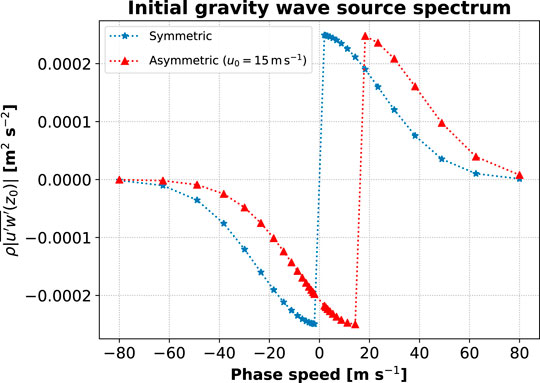
FIGURE 1. Default gravity wave spectrum launched at the source pressure level (p = 100 hPa, $\sim 15$ km) plotted as a function of harmonic’s horizontal phase speed. The blue and red curves show the symmetric and asymmetric spectra, respectively. The symmetry property of the spectrum is dependent on the variations of the wind at the source level $u_0=\overline{u}\left(z_0\right)$, which is assumed to be 15 m s⁻¹ in the figure for illustrative purposes. In the GCM, $u_0$ has spatiotemporal variability. The spectral parameters of the standard spectrum are as follows: $c_w=35$ m s⁻¹ and $\overline{u^{\prime }{w}^{\prime }}$_max = 2.5 × 10⁻³ m² s⁻². M = 34 harmonics are used.

In the rest of the paper, this default spectrum will be modified using TIMED/SABER observations as a guide, and the response of the middle and upper atmosphere will be studied in sensitivity tests.

2.4 Model Simulations and Experiment Design

The GCM was run from March equinox to May 1, 2010, which was subsequently used as the start-up point for all test simulations. We use the asymmetric default spectrum, i.e., with variable source winds, in the simulations to be presented in this paper. Then, simulations continued till the end of July 2010, assuming constant spectral parameters listed in the previous section (hereafter referred to as experiment EXP0). The subsequent simulations have been performed with the modifications of the source motivated by the previously observed hemispherically asymmetric distribution of GW activity in the lower stratosphere (e.g., Geller et al., 2013; Ern et al., 2018). For this, we take as a proxy the latitudinal variation of the GW activity observed by SABER in the lower atmosphere. Model data are output every 3 h during the June-July period. These 3 h outputs are used for all the longitudinal (zonal) and 60-day time averages to be presented.

2.5 Adjustment of the Source Spectrum

We adopt different latitudinal shapes of the source momentum flux in the troposphere, using SABER observations in the stratosphere as a guide. This is achieved by adjusting the magnitude of the momentum flux in the source spectrum as

$\overline{u^{\prime }{w}_{\mathit{max}}^{\prime }}\left(\theta \right)=\overline{u^{\prime }{w}_{\mathit{max}}^{\prime }}\times \left[1+A{\sin }^4\left(2\theta \pm \Delta \theta \right)\right],(16)$

where θ is the latitude, A is the adjustment coefficient, and $\text{Δ}\theta$ specifies the latitudinal shift of the peak. $A=0$ corresponds to the standard spectrum (EXP0). $A>0$ with $\text{Δ}\theta =0$ yields a sinusoidal dependence that peaks at $\pm 45\text{°}$, as shown in Figure 2 for $A=0.5$ (cyan curve). For sensitivity experiments, we selected two additional setups that bring the source closer to observations, while incrementally demonstrating associated changes in the middle and upper atmosphere. In EXP1, we introduce a southward latitudinal shift of the peak by $\text{Δ}\theta =10\text{°}$, while preserving the overall sinusoidal distribution in latitude. Further, we assume a 50% increase of the momentum flux magnitude in both hemispheres (A = 0.5). In EXP2, we repeat EXP1 but increase the benchmark source strength in the Southern Hemisphere (SH) by 100% and adopt this as the amplitude of the sinusoidal variation, as seen in Figure 2, resulting in a hemispheric asymmetry not only in the location of the peak momentum flux but also in terms of the peak source strength of GW fluxes. Note that scaling the maximum source strength also equally scales the total absolute momentum flux Eq. 8 contained in the spectrum.

FIGURE 2

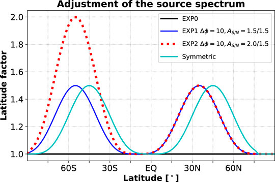
FIGURE 2. Latitudinal factors used in the GW source spectrum for the maximum source momentum flux at 15 km, $\overline{u^{\prime }{w}^{\prime }}$_max, in simulations EXP0, EXP1, and EXP2, plotted in terms of how much the peak source momentum flux has been increased, somewhat mimicking the variations seen in SABER GW momentum flux observations. EXP0 (black) is the standard spectrum used in the parameterization. EXP1 (blue) assumes a sinusoidal variation of the maximum source flux with an amplitude of 50% increase with respect to EXP0 (hence the factor 1.5) and shifted by 10 degrees southward. EXP2 (red dashed) is similar to EXP1, but the maximum source flux is doubled in the Southern Hemisphere (i.e., $A_{S/N}=2.0/1.5$).

3 Comparison With Observed Wave Activity in the Stratosphere and Mesosphere

We next compare in Figure 3 the GW activity modeled in the three experiments with SABER observations. This is done for three vertical levels in the stratosphere and mesosphere for June-July 2010 conditions. The mean total absolute momentum flux calculated with Eq. 8 for EXP0 (black), EXP1 (blue), and EXP2 (red), as well as SABER absolute momentum fluxes (green), is shown with different colors, while the different line styles represent the fluxes at 15 km (solid line), 32.5 km (dashed line), and 87.5 km (dotted line). The fluxes at the last two vertical levels are averaged in 5 km vertical bins centered around the respective levels for intercomparison between the model and data.

FIGURE 3

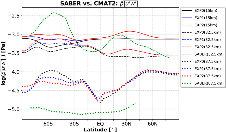
FIGURE 3. Comparison of the modeled zonal mean total absolute horizontal momentum flux among the different experiments and SABER at 15 km (solid line), 32.5 km (dashed), and 87.5 km (dotted). The model simulations, EXP0 (black), EXP1 (blue), and EXP2 (red), are represented by different colors.

In the stratosphere, not only is the modeled GW activity overall smaller compared to SABER, but also the simulated latitude variations are rather weak in the benchmark run. This is expected to be, as SABER observes a broad range of wavelengths, while the parameterization considers only small-scale GWs with the characteristic horizontal wavelength of 300 km. Nevertheless, the modeled GW activity is similar to SABER at low latitudes and NH high latitudes. The observations show overall a more pronounced hemispheric difference, with GW activity peaking around midlatitudes and with stronger GW activity in the SH. Close inspection shows that the observed latitudinal variation of GW activity appears to be close to the sinusoidal shape with two peaks in the midlatitudes somewhat shifted southward away from $\pm 45\text{°}$. It is also seen that the modeled GW activity significantly evolves from 15 to 32.5 km in terms of magnitude and latitude structure, mainly owing to lower atmospheric filtering of slow phase speed harmonics from the incident spectrum. Introducing a sinusoidally varying latitude-dependent modulation with peaks situated at 55°S and 35°N (EXP1) improves the comparison of the fluxes with SABER. Doubling the SH peak flux in EXP2, while keeping the NH values the same as in EXP1, introduces the hemispheric asymmetry in both the magnitude and location of the peaks similar to what is observed by SABER. This makes the comparison with SABER more favorable.

In the mesosphere, the modeled fluxes are larger than the observed, especially at midlatitudes, and the response of the fluxes to the source modulation is not linear. Thus, increasing the source flux in a latitude-depend manner in EXP1 and EXP2 produces smaller wave activity at these altitudes. This is primarily due to the enhanced nonlinear dissipation as a consequence of increased interaction of harmonics having larger amplitudes in the middle atmosphere. The best comparison with the observations is achieved in EXP2, where the mesospheric GW flux smoothly varies with latitude, reminiscent of the SABER data. SABER is less reliable in the cold summer mesopause region, where the retrieval noise is relatively large (Ern et al., 2018; Figure 7). Therefore, the data poleward of 40°N are not included in the above analysis.

Different from the stratosphere, SABER absolute momentum fluxes at 87.5 km altitude are lower than the parameterized momentum fluxes. The likely reason is that SABER underestimates the contribution of short horizontal wavelength GWs that become more important in the mesopause region.

As the model is forced by NCEP and GSWM data at the lower boundary, it is important to note that the source level winds are time-dependent and vary with geographical location. Hence, the momentum flux distribution at the lower boundary is expected to be time-dependent and geographically variable as well, despite the fact that all the spectral parameters in the asymmetric default spectrum are kept constant. We next explore how changes in the GW sources in the troposphere modify the simulated circulation in the middle and upper atmosphere.

4 Mean Zonal Winds

Figure 4 presents the time-mean zonal mean winds (hereafter referred to as mean zonal winds) for the three model simulations: a) the benchmark run with the standard GW spectrum EXP0, b) the run with the latitude-dependent sinusoidal spectrum, 10° southward shift, increased by 50% with respect to the benchmark run magnitude in both hemispheres (EXP1), and c) the run with the latitude-dependent spectrum (as in EXP1), but increased by a factor of 2 (i.e., by 100%) fluxes in the SH. For comparison, the UARS mean zonal winds are shown in panel d (see also Swinbank and Ortland, 2003).

FIGURE 4

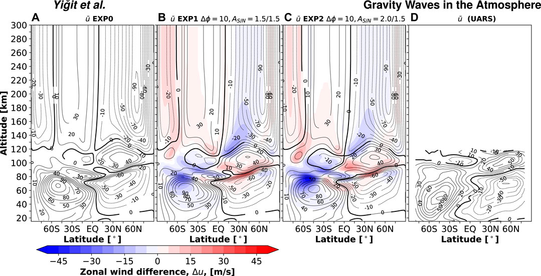
FIGURE 4. Zonal mean winds (black contours) and differences (color shading) for the 2010 June-July period: (A) EXP0: benchmark simulation; (B) EXP1: using sinusoidally varying GW spectrum with a factor of 1.5 enhancement of the peak horizontal momentum flux in both hemispheres and a southward latitudinal shift of 10° with respect to EXP0; (C) EXP2: the same as EXP1 but with a factor of 2 enhancement in the SH; (D) UARS winds. The contour intervals for the zonal winds and wind differences are 10 m s⁻¹ and 5 m s⁻¹, correspondingly. The differences between a given run (EXP1 or EXP2) and the benchmark run (EXP0) are shown, i.e., EXP1-EXP0 and EXP2-EXP0.

During the considered solstice season, the circulation in the middle atmosphere consists of the westerlies in the winter SH and easterlies in the summer NH. They are maintained by the Coriolis torque associated with the large-scale summer-to-winter meridional circulation cell. Above, in the upper mesosphere, the GW momentum forcing produces reversals of the jets that are captured by the model at around $\sim 90-100$ km. In the NH, they are located slightly lower in altitude and are stronger than in the SH (50 m s⁻¹ vs. 10 m s⁻¹) as shown in all the simulations. These features grossly agree with the UARS winds averaged over June and July. It is those relatively subtle differences associated with modifications of GW sources, which are of our interest.

Simulation EXP1 produces significant global changes in the mean zonal winds above 60 km, especially in the region poleward of midlatitudes in the SH, around the tropical region, and in the midlatitudes of the NH. Thus, the winter westerlies are slowed down by about 20 m s⁻¹ in EXP 1 around $60\text{°S}$ in the mesosphere. This effect is even stronger in EXP2, where the source GW flux was larger.

Significant changes are seen also around equatorial latitudes in the MLT. Increasing the magnitude of the source momentum flux and shifting southward its sinusoidal latitude distribution increases the equatorward tilt of the eastward mesospheric jet in the SH, bringing the wind fields in better agreement with observations. The agreement is even better if the source flux is magnified in the SH more than in the NH, as done in EXP2. This brings the simulated jet closer to the observed structure with ∼10 m s⁻¹ winds around the equator at 95 km.

The basic structure of the thermospheric circulation resembles that in the middle atmosphere, but its magnitude and distribution are strongly modified via interactions with the ionosphere and with sources of magnetospheric origin. In the high-latitude thermosphere above the turbopause, zonal winds and meridional winds are affected by Joule heating (Rodger et al., 2001) and particle precipitation, in addition to the Coriolis torque associated with the mean meridional summer-to-winter circulation. The Joule heating is in turn is influenced by the distribution of neutral winds (Thayer, 1998). If forcing by GWs is not accounted for, the jets in the mesosphere reverse back above ∼120 km, and the pattern of the thermospheric zonal winds replicates that in the stratosphere, strongly modified by the ion drag. Inclusion of GW effects in the “whole atmosphere parameterization” modifies the simulated winds in the thermosphere, as was previously discussed (Yiğit et al., 2009), nudging them closer to the observationally based Horizontal Wind Model (HWM, Hedin et al., 1996). In particular, they weaken the westerly jet in the winter SH and even reverse it to easterlies in high latitudes. Introducing the latitudinal dependence and increasing the magnitude of the GW sources in the lower atmosphere produces a noticeable but less dramatic effect in the upper thermosphere. As is seen in Figures 4B,C, GWs impose a drag on the zonal winds at high latitudes of both hemispheres and accelerate them in other regions. The associated magnitude of the wind changes varies between $\pm 10$ m s⁻¹ and depends on latitude.

5 Gravity Wave-Induced Dynamical Effects and Temperature Fluctuations

To elucidate the effects of GWs, we plotted the associated zonal momentum forcing in Figure 5. The GW drag represents a major source of the zonal momentum in the MLT and significantly contributes to the momentum budget of the thermosphere. This is clearly seen in the presented model simulations. The mean westward GW drag of 160 m s⁻¹ day⁻¹ at around 80 km in the SH midlatitudes and eastward drag of more than ∼200 m s⁻¹ day⁻¹ are responsible for the reversal of the mean mesospheric zonal winds shown in Figure 4. In the thermosphere, the strong eastward GW forcing concentrates at high latitudes of both hemispheres with larger values in the NH. This agrees with previous modeling studies using parameterized GWs (e.g., Yiğit et al., 2009) and GW-resolving GCMs (e.g., Miyoshi et al., 2014).

FIGURE 5

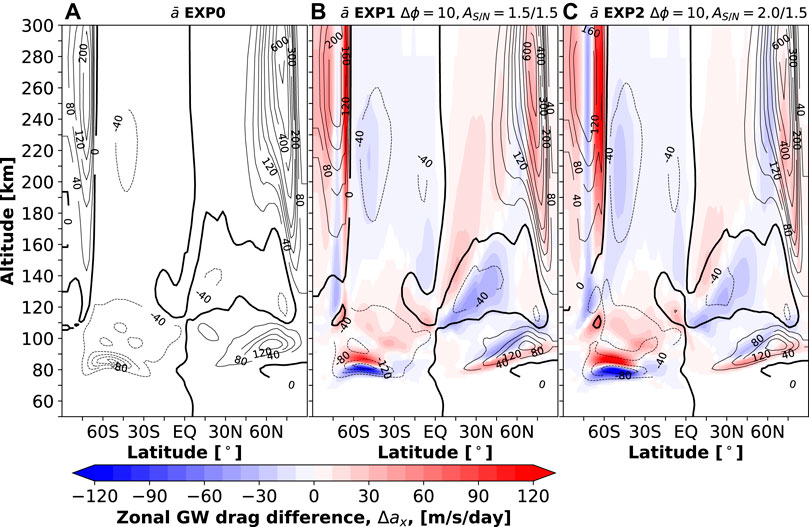
FIGURE 5. same as in Figures 4A–C, but for the zonal mean GW drag. The contour intervals are 40 m s⁻¹ day⁻¹ between $\pm 200$ m s⁻¹ day⁻¹ and 100 m s⁻¹ day⁻¹ for the drag values with magnitudes larger than 200 m s⁻¹ day⁻¹.

The color shades in Figure 5 highlight the changes in the zonal GW drag introduced by the modification of GW sources in the troposphere. In the MLT, the midlatitude westward drag strengthens at lower altitudes and weakens at higher altitudes, as indicated by the alternating red and blue patterns. This effect is more pronounced in EXP2, where the source flux was further increased in the SH. Accordingly, the GW drag above the turbopause is enhanced as well to a larger degree in the high latitudes of the SH compared to the NH. The 40 m s⁻¹ day⁻¹ increase of the westward forcing at low latitudes around 100–150 km in the NH clearly correlates with the acceleration of the westward wind in this region as seen in Figure 4.

Further insight into the wave activity can be gained by studying temperature fluctuations $\left|T^{\prime }\right|={\left(\overline{T^{\prime 2}}\right)}^{1/2}$ induced by the upward propagating GWs. They are presented in Figure 6 along with those retrieved from SABER observations. While GW drag provides directional information on the wave field, $\left|T^{\prime }\right|$ is a scalar that characterizes a global picture of GW activity. In the mesosphere, it is larger in the midlatitudes. The maximum values of $\left|T^{\prime }\right|=6$ K and 8 K occur in the SH and NH, respectively, with the latter located somewhat higher, similar to the behavior of the zonal GW drag. In the thermosphere, GW-induced temperature fluctuations are much larger, especially at the low and high latitudes in both hemispheres. Specifically, the regions of the largest activity are seen around 120–130 km, the equator ($\left|T^{\prime }\right|\sim 12$ K), at 120 km around $75\text{°S}$ ($\left|T^{\prime }\right|\sim 14$ K), and between 200 and 280 km around $75\text{°N}$ ($\left|T^{\prime }\right|\sim 22$ K).

FIGURE 6

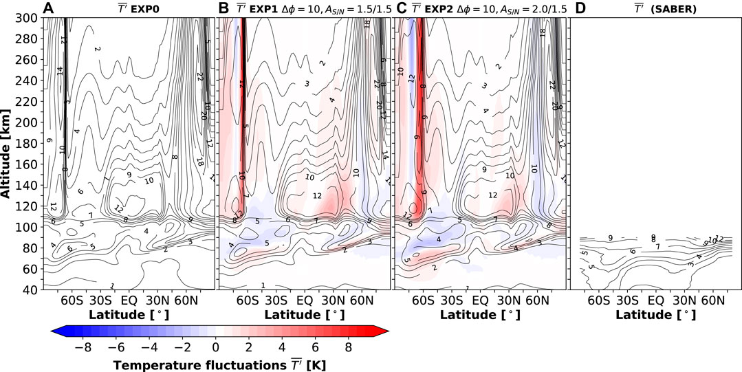
FIGURE 6. same as in Figures 4A–C, but for the GW-induced temperature fluctuations $\left|T^{\prime }\right|$. The SABER GW activity is shown in panel (D). The contour intervals are 1 K between $\left|T^{\prime }\right|=1-9$ K and 2 K between $\left|T^{\prime }\right|=10-22$ K.

Modifications of the GW flux at the source level in the troposphere (EXP1 and EXP2) produce some changes in the SH above 60 km and in the tropics above 80 km. Poleward of 60°S in the lower mesosphere, the magnitude of temperature fluctuations increases, while it decreases in the upper mesosphere. This effect is more evident when the source flux is further increased in the SH (EXP2). Figure 6D presents the associated SABER temperature fluctuations between 30 km and 90 km. It shows a more latitudinally uniform distribution of $\left|T^{\prime }\right|$ in the mesosphere. The model predicts slightly larger $\left|T^{\prime }\right|$ at midlatitudes than at low latitudes. Apart from these differences, the magnitudes of the simulated temperature fluctuations of ∼ 6–7 K in the middle atmosphere are compatible with the SABER values. Note that the latter greatly exceeds the former in the troposphere and stratosphere. The explanation for this behavior is discussed further in the text.

6 Mean Temperature

The mean temperature distribution for the 2010 June-July average is seen in Figure 7, presented in the same manner as the mean fields above, along with the retrieved SABER temperatures. All runs reproduce the reversal of the meridional temperature gradient in the mesosphere, where the summer mesopause is colder than the winter one owing to the GW momentum deposition and associated changes in the mean meridional circulation and adiabatic heating/cooling. The additional runs with modified GW source spectrum both consistently show changes of the mean temperature above 40–60 km. The greatest effects are seen in the middle atmosphere at SH high latitudes. There, between 40 and 70 km in the upper stratosphere and mesosphere, the simulated temperature increases up to $\sim 15$ K in EXP1 and more than 27 K in EXP2, while above 70 km up to 120 km, the temperature is lower by up to 10 K and 14 K in EXP1 and EXP2, respectively. Higher up in the thermosphere, there is a cooling of −4 to −8 K. While relative temperature changes in the middle atmosphere are in the order of $\pm 10\text{\%}$, they are much smaller (around $-1$ to $-2\text{\%}$) in the thermosphere. In the summer mesopause, the modeled mean temperature is slightly lower than that measured by SABER. However, the overall mean temperature distribution is in good agreement with SABER observations up to 110 km.

FIGURE 7

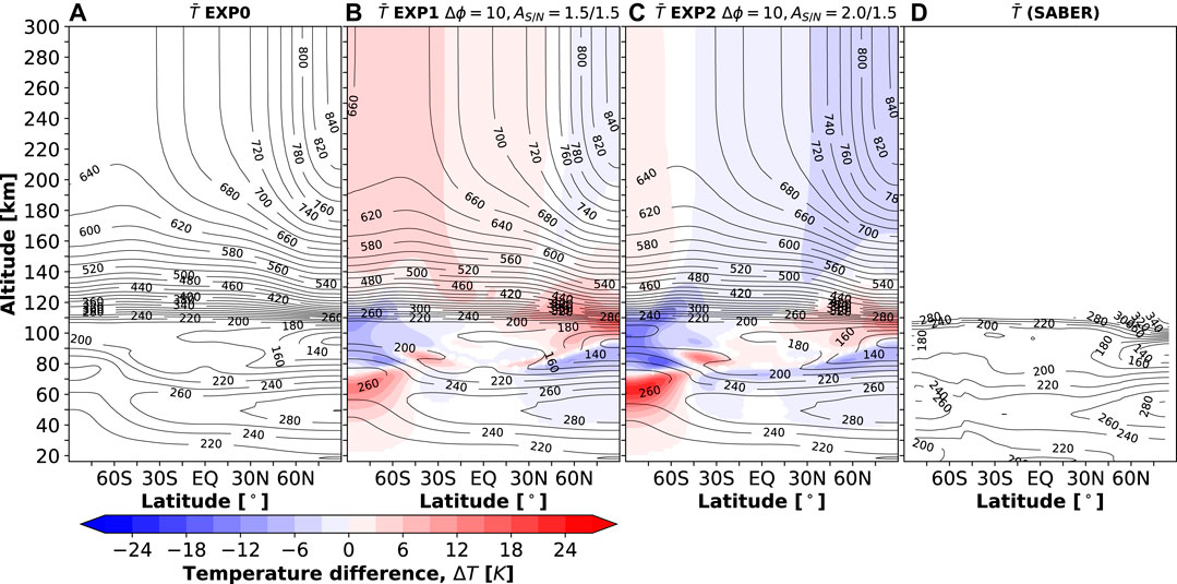
FIGURE 7. Panels (A)–(C) are the same as in Figure 4, but for the neutral temperature in K. Simulations are compared to the SABER temperatures in (D).

7 Mean Gravity Wave Thermal Effects

GW-induced heating/cooling rates are shown in Figure 8 in the same manner as in the previous figures for the mean fields. The majority of the thermal effects are concentrated at high latitudes in the thermosphere, while some are seen in the upper mesosphere and lower thermosphere. GWs mainly heat the middle thermosphere and cool the upper thermosphere (Yiğit and Medvedev, 2009). There is a visible hemispheric asymmetry in GW thermal effects with clearly larger values in the NH than SH, following the distribution of the GW dynamical effects and GW activity. Around 120 km in the high-latitude SH, a localized region of large GW cooling is seen along with a region of cooling in the low-latitude lower thermosphere of up to −20 K day⁻¹. While all three simulations produce a similar global distribution of GW thermal effects, some differences are seen in their magnitudes. Again, the main differences are in the high-latitude SH. Around 120 km in the high-latitude SH, the localized cooling intensifies from −20 K day⁻¹ to −30 K day⁻¹ in EXP1 and to −40 K day⁻¹ in EXP2. At higher altitudes, shifting the GW sources southward produces relative warming in the middle thermosphere and relative cooling in the upper thermosphere, especially in the SH high-latitude above 240 km. Theoretical discussions of GW heating/cooling rates in terms of the divergences of the sensible heat flux and energy flux associated with viscous stresses can be found in the works by Medvedev and Klaassen (2003) and Hickey et al. (2011).

FIGURE 8

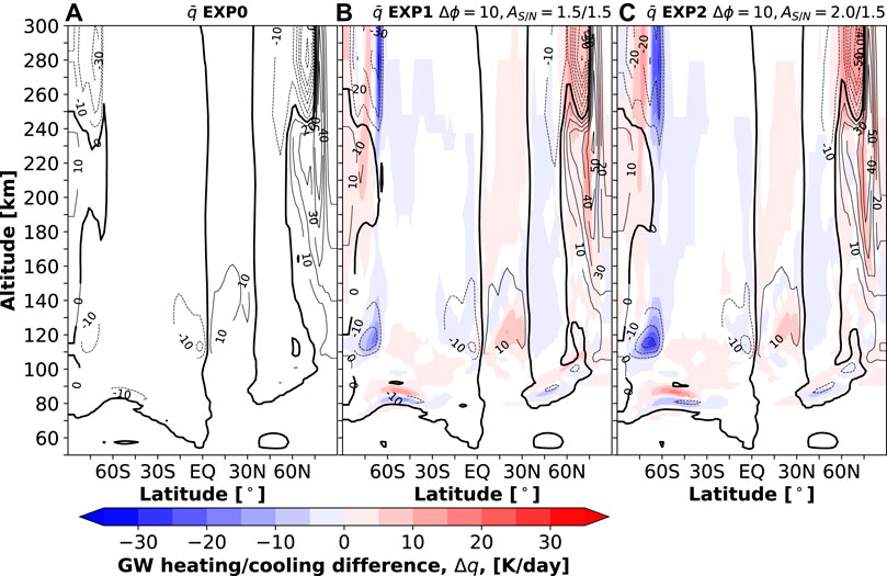
FIGURE 8. Panels (A)–(C) are the same as in Figure 4, but for the GW heating/cooling rates. The contour intervals are 10 K day⁻¹ between $\pm 50$ K day⁻¹ and 20 K day⁻¹ for values with magnitudes larger than 50 K day⁻¹.

8 Discussion

8.1 Comparison of Gravity Wave Momentum Flux with SABER Observations

While SABER serves as a powerful tool to study the global climatology of GW activity, in fact, it should be used with caution for validating model GW fluxes because of a number of reasons. First, in SABER, the total absolute momentum flux is a derived quantity that relies on the GW polarization relations, while in our modeling, we prescribe GW activity in terms of momentum fluxes for each GW harmonic as $\overline{u^{\prime }{w}^{\prime }}\left(c_i\right)$ (Eq. 15). There are alternative ways of defining GW activity, for example, in terms of momentum flux spectra as functions of frequency and wavenumbers (e.g., Tsuda et al., 2000; Orr et al., 2010). Second, high-quality reliable SABER GW data do not extend all the way down to the lower boundary of the model, which is at ∼15 km. Third, SABER captures a broader range of wavelengths than what is considered in the GCM, as we specifically parameterize subgrid-scale GWs with a representative horizontal wavelength of 300 km. Among others, these SABER characteristics should be kept in mind while comparing with models. One could technically launch the GW spectrum at 30 km using the SABER fluxes. However, not only would this be an overestimation of the modeled subgrid-scale GW activity but also the alternative launch level would be relatively far away from the primary tropospheric sources of those nonorographic GWs that have dynamical importance for the middle and upper atmosphere. Primary GW sources are due to a combination of various meteorological processes, often a mixture of orographic and nonorographic sources, such as topographic forcing (Nastrom and Fritts, 1992), convection (Song et al., 2003; Beres et al., 2004; Song and Chun, 2008; Kherani et al., 2009), fronts (Fritts and Nastrom, 1992; Gall et al., 1988; Reeder and Griffiths, 1996; Charron and Manzini, 2002; Plougonven and Zhang, 2014; Wei and Zhang, 2014), and tornadoes (Hung et al., 1979). It is important to note that the GW scheme exclusively accounts for GWs unresolved by the GCM, whose scales depend on the model resolution, while SABER observes a broad range of GW scales. In the stratosphere, larger-scale inertia GWs can play an important role. These waves are resolved in the model to some extent, rather than being parameterized. Note that the inertia GWs contribute to the observed SABER momentum flux at 30 km at the longer wavelength part. Therefore, the most instructive approach for our purpose was to use a sinusoidal function that mimics the latitudinal variation of GW activity in the lower atmosphere as observed by SABER and other satellite instruments and as simulated by high-resolution global models. The notion of latitudinal distribution can also be interpreted as a seasonal cycle since our simulations focus on the boreal summer solstice. We also rely on the recent findings, which all indicate a latitudinal variation, such as SABER and HIRDLS satellite observations that are sensitive to horizontal wavelengths $>100-200$ km and vertical wavelengths in the range 2–25 km (Ern et al., 2018); dedicated high-resolution convection-permitting model simulations by ICON, NICAM, and IFS (Stephan et al., 2019a, b) that resolve horizontal wavelength >50 km and vertical wavelengths greater than 2 km; and AIRS satellite observations of GWs that are sensitive to horizontal wavelengths >30 km and vertical wavelengths $>15$ km (Ern et al., 2017; Meyer et al., 2018). All these datasets are sensitive to very different parts of the GW spectrum, but nevertheless they show similar latitudinal distributions/seasonal cycles of GW activity. Therefore, we assume that similar relative variations are also applicable to the gravity wave parameterization in CMAT2.

While the latitudinal variations of GW momentum fluxes are similar in satellite observations and high-resolution model simulations (e.g., Geller et al., 2013; Stephan et al., 2019a; Stephan et al., 2019b), with the latter being widely independent of the resolved GW horizontal scales, average horizontal wavelengths of GWs observed by SABER are comparably long. Partly, this is due to the large spectral range covered by SABER. In addition, only along-track horizontal wavelengths (i.e., parallel to the direction of the measurement track) can be derived from SABER observations. They overestimate the true GW horizontal wavelength and thus underestimate the momentum flux in a way that varies systematically with latitude. Average horizontal wavenumbers for boreal summer observed by SABER can be seen from the climatology shown in the paper by Ern et al. (2018), Figure 10c. The average zonal wavenumbers given there correspond to an along-track horizontal wavelength of about 1,000 km at 30 km altitude and to about 1,500 km in the mesopause region. As was argued by Ern et al. (2017), the true GW horizontal wavelengths might be about a factor of two shorter waves (i.e., 500 km and 750 km, respectively).

Only absolute momentum fluxes can be derived from SABER observations. This makes direct comparison with parameterized GW momentum fluxes more difficult. The purpose of a GW parameterization is to accurately simulate net momentum fluxes because net momentum fluxes are relevant for the interaction of GWs with the background flow. Net momentum fluxes are calculated from the parameterization by summing up the different spectral components that are launched in different directions. Still, there could be GWs in the real atmosphere which contribute to absolute momentum fluxes but cancel in net momentum fluxes and are not needed in the parameterization and therefore may not be accounted for. Note that the forcing in the model produced by breaking/dissipating GW harmonics propagating along the local wind in opposite directions exactly cancels each other, while their contributions to the wave activity would sum up. If the goal was solely to match the simulated and observed GW activity in the troposphere and lower stratosphere, one could introduce at the launch level harmonics propagating in various directions. However, these waves would have very little contribution to the momentum forcing, especially in the lower layers in the stratosphere, and are largely filtered out by the varying mean winds on their way up to the mesosphere and above. In addition, SABER is sensitive only to GWs with relatively long horizontal wavelength. Therefore, the magnitudes of SABER absolute momentum fluxes and of parameterized absolute momentum fluxes are not directly comparable. Still, the agreement between the modeled and observed GW activity/temperature variations in the upper atmosphere is much better than that around the launch level, which indicates that, in addition to the realistic net forcing of the background flow, also simulated GW heating/cooling rates should become more and more realistic with altitude. Overall, SABER can serve as a good proxy of GW activity and can be used by models for that purpose, depending on the kind of the model, what kind of waves are parameterized, and on what kind of waves are resolved.

8.2 Gravity Wave Drag Versus Gravity Wave Activity

GW activity, for example, in terms of temperature fluctuations (Figure 6) and drag (Figure 5), characterizes different aspects of the wave field. First, while the wave activity is a measure of the presence and magnitude of harmonics in a given point, GW drag is related to their dissipation and vertical decay. Freely propagating waves show vertically growing activity and produce no drag. On contrary, in the regions where GWs dissipate and/or break, the activity reduces, and drag imposed on the mean flow by each harmonic of the spectrum is no longer zero. Second, the wave activity is a positively defined quantity, while the drag is a vector. Thus, two dissipating harmonics propagating in opposite directions and carrying large momentum fluxes of opposite signs could cancel each other’s effects, yielding no net dynamical effect on the mean flow. However, GW activity in the same region can be totally different, since their contributions are summed up. For example, the body force per unit mass produced by dissipating GWs at low latitudes is much smaller than that at high latitudes (Figure 5); however, the associated GW activity is comparable to the high-latitude values.

The example above illustrates how consideration of both GW drag and variance can provide an insight into GW processes in the atmospheres. In the middle-to-high-latitude region, GW harmonics encounter enhanced wind filtering by the underlying strong atmospheric winds. Waves from the broad spectrum traveling against the background wind would then survive filtering and reach higher altitudes relatively unattenuated. Upon breaking/dissipation at large amplitudes (large $\left|T^{\prime }\right|$), they impose a large drag on the mean flow. In the tropics, the mean winds are significantly weaker, and their directions alternate with height. A portion of GW harmonics with phase speeds exceeding the local wind then evade filtering and reach the mesosphere and thermosphere, yielding a significant amount of $\left|T^{\prime }\right|$ (Figure 6). However, the momentum deposited by harmonics moving in opposite directions cancel each other to a certain degree; thus, the total GW drag is relatively small at low latitudes (Figure 5).

A significant amount of atmospheric GW observations characterizes GW activity by studying temperature or density perturbations and the resulting wave potential energy per unit mass (e.g., Wilson et al., 1990; Tsuda et al., 2000; John and Kumar, 2012; Yue et al., 2019). While these quantities provide a highly needed picture of the intensity of GWs in the atmosphere, variations of the wave fluxes as well as background winds have to be considered in order to gain a more complete picture of GW dynamics. Studying GW processes with GCMs constrained by observations can provide insight into both aspects of GW fields, the activity and dynamics.

8.3 Spectral Shift of the Source Spectrum

Due to the complexity of small-scale GW processes, GW schemes typically use a uniform and homogeneous distribution of wave activity, described in terms of momentum fluxes as functions of phase speed. However, even in the benchmark case (EXP0), where the constant source strength $\overline{u^{\prime }{w}_{\mathit{max}}^{\prime }}$ is used, the geographical distribution of the wave stress in the model is not constant but exhibits a nonnegligible variability due to temporal changes of the lower boundary winds, which affects the intrinsic phase speed at different locations. The adopted latitude-dependent GW source introduces variations of flux magnitudes but does not change the intrinsic phase speeds at the lower boundary. Meanwhile, these phase speeds are of great importance for the GW activity and associated dynamical and thermal effects. They explicitly enter the expressions for the vertical damping rates β and, thus, affect the transmissivity τ (Eq. 5)). The Doppler shift by the varying mean winds (and subsequent change of τ) is responsible for multiple GW-induced phenomena in the middle atmosphere, such as semiannual and quasibiennial oscillations and zonal jet reversals in the mesosphere.

The horizontal wavelength of GWs in this parameterization is set to a representative value of 300 km, to which an important portion of the small-scale GW activity can be statistically attributed. The horizontal wavelength ${\lambda }_h$ enters nonlinearly the expressions for the vertical damping rates β due to all major dissipative mechanisms (see Yiğit et al., 2008, Section 3), on which the GW drag depends linearly (Yiğit et al., 2008, Eq. 5). In general, the GW forcing is nonlinearly proportional to ${\lambda }_h$: shorter waves produce stronger forcing at a given momentum flux. The sensitivity of the GW parameterization has been tested in the paper by Yiğit et al. (2009) and demonstrated that the simulation results depend little on the horizontal wavelength, considering the typical ranges of a few hundred kilometers. Of course in a realistic atmosphere, it is possible that there are multiple wavelengths present at a given moment; however, our results in the mesosphere and thermosphere are less sensitive to the variations of ${\lambda }_h$ compared to other parameters. From the perspective of GW propagation and dissipation within the context of coarse-grid GCMs, the most important two aspects are 1) an accurate representation of physics of GW dissipation and 2) intrinsic horizontal phase speed of GWs.

Our simulations show that a significant increase in the source strength produces fewer effects in the thermosphere compared to the middle atmosphere, as GW propagation there is controlled by the competition between the variation of the intrinsic phase speed and increase of molecular diffusivity with height. In the MLT region, GW effects are more sensitive to the variation of the source, since the increased source flux appreciably enhances nonlinear dissipation acting on the harmonics in the mesosphere. The latter manifests itself by the downward shift of the GW drag and activity maxima.

9 Summary and Conclusion

We have presented simulations with the mechanistic Coupled Middle Atmosphere-Thermosphere-2 (CMAT2) general circulation model (GCM) (Yiğit et al., 2009), incorporating the whole atmosphere subgrid-scale GW parameterization of Yiğit et al. (2008). It was used for studying the response of the simulated mean fields and GW activity from the tropopause to the upper thermosphere to observationally guided variations of GW sources in the lower atmosphere. For that, we incorporated a latitude-dependent GW source activity that resembles the one observed by TIMED/SABER in the lower atmosphere and explored the mesospheric and thermospheric effects of upward propagating GWs. As a first approach, we have investigated the boreal summer season. The main findings of our study can be summarized as follows:

(1) The SABER observations of GW activity in the lower atmosphere suggest a distinct hemispheric asymmetry in the magnitude and location of the peak of absolute momentum fluxes. These hemispheric differences are due to a combination of seasonal differences and ocean-land contrasts.

(2) In order to mimic the observed total GW absolute momentum flux variations, we implemented a latitude-dependent GW source spectrum that varies sinusoidally and whose peaks can be adjusted to account for the observed hemispheric asymmetry. Increasing the source magnitude and shifting the peaks by 10 degrees southward, somewhat resembling the SABER data, produce noticeable changes in the mean circulation above 60 km, especially in the region poleward of midlatitudes in the SH.

(3) Various formulations of GW activity, such as temperature fluctuations or (zonal) drag, characterize different aspects of the wave field. While the activity is a measure of the presence and magnitude of harmonics in a given point, GW drag is related to their dissipation and vertical decay.

(4) GW activity and associated dynamical and thermal effects strongly depend on the vertical structure of the horizontal momentum flux. SABER observations provide GW activity in terms of absolute momentum fluxes, which do not include directional information, while the GW parameterization specifies the GW activity in terms of vector fluxes and phase speeds.

(5) While SABER observes a broad range of wavelengths, including rather longer ones, GW parameterizations explicitly model small-scale harmonics assuming a single representative wavelength. As parameterizations only have to account for the nonresolved part of the GW spectrum, the total absolute momentum flux is smaller in the GW parameterization source spectrum than in the observations. In addition, the purpose of GW parameterizations is to model net GW momentum fluxes to correctly simulate the forcing of the background atmosphere by GWs. Absolute momentum fluxes can be considerably stronger if cancellation effects occur due to GWs that contribute to the absolute but not to the net momentum fluxes.

(6) In the middle and upper atmosphere, the agreement between the modeled and observed wave activity is better. This occurs because the parameterization captures a portion of GW harmonics that penetrates to upper layers and produces relevant dynamical effects there.

(7) The response of the large-scale circulation in the middle and upper thermosphere is less sensitive to latitudinal variations of the GW source spectrum than in the mesosphere and lower thermosphere.

Future studies can consider possible effects of longitudinal variations in GW sources in the lower atmosphere.

Data Availability Statement

The datasets presented in this study can be found in online repositories. The names of the repository/repositories and accession number(s) can be found at https://doi.org/10.5281/zenodo.3908471.

Author Contributions

EY performed the model simulations and model data analysis and wrote the first draft of the paper. ME provided SABER GW analysis and edited the paper. AM and ME contributed significantly to the analysis and writing process.

Funding

The work of ME was supported by Deutsche Forschungsgemeinschaft (DFG, German Research Foundation) project ER 474/4-2 (MS-GWaves/SV) within the DFG research unit FOR 1898 (MS-GWaves) and DFG project ER 474/3-1 (TigerUC) within the DFG priority program SPP-1788 (“Dynamic Earth”).

Conflict of Interest

The authors declare that the research was conducted in the absence of any commercial or financial relationships that could be construed as a potential conflict of interest.

References

Alexander, M. J., and Barnet, C. (2007). Using satellite observations to constrain parameterizations of gravity wave effects for global models. J. Atmos. Sci. 64, 1652–1665. doi:10.1175/jas3897.1

CrossRef Full Text | Google Scholar

Alexander, M. J., Geller, M., McLandress, C., Polavarapu, S., Preusse, P., Sassi, F., et al. (2010). Recent developments in gravity-wave effects in climate models and the global distribution of gravity-wave momentum flux from observations and models. Q. J. R. Meteorol. Soc. 136, 1103–1124. doi:10.1002/qj.637

CrossRef Full Text | Google Scholar

Beres, J. H., Alexander, M. J., and Holton, J. R. (2004). A method of specifying the gravity wave spectrum above convection based on latent heating properties and background wind. J. Atmos. Sci. 61, 324–337. doi:10.1175/1520-0469(2004)06110.1175/1520-0469(2004)061<0324:amostg>2.0.co;2

CrossRef Full Text | Google Scholar

Chanin, M.-L., and Hauchecorne, A. (1981). Lidar observation of gravity and tidal waves in the stratosphere and mesosphere. J. Geophys. Res. 86, 9715–9721. doi:10.1029/jc086ic10p09715

CrossRef Full Text | Google Scholar

Charron, M., and Manzini, E. (2002). Gravity waves from fronts: parameterization and middle atmosphere response in a general circulation model. J. Atmos. Sci. 59, 932–941. doi:10.1175/1520-0469(2002)059<0923:gwffpa>2.0.co;2

CrossRef Full Text | Google Scholar

Ern, M., Hoffmann, L., and Preusse, P. (2017). Directional gravity wave momentum fluxes in the stratosphere derived from high-resolution AIRS temperature data. Geophys. Res. Lett. 44, 475–485. doi:10.1002/2016GL072007

CrossRef Full Text | Google Scholar

Ern, M., Preusse, P., Alexander, M. J., and Warner, C. D. (2004). Absolute values of gravity wave momentum flux derived from satellite data. J. Geophys. Res. 109, D20103. doi:10.1029/2004JD004752

CrossRef Full Text | Google Scholar

Ern, M., Preusse, P., Gille, J. C., Hepplewhite, C. L., Mlynczak, M. G., Russell, J. M. R, et al. (2011). Implications for atmospheric dynamics derived from global observations of gravity wave momentum flux in stratosphere and mesosphere. J. Geophys. Res. 116, D19107. doi:10.1029/2011JD015821

CrossRef Full Text | Google Scholar

Ern, M., Preusse, P., and Warner, C. D. (2005). A comparison between CRISTA satellite data and warner and mcintyre gravity wave parameterization scheme: horizontal and vertical wavelength filtering of gravity wave momentum flux. Adv. Space Res. 35, 2017–2023. doi:10.1016/j.asr.2005.04.109

CrossRef Full Text | Google Scholar

Ern, M., Trinh, Q. T., Kaufmann, M., Krisch, I., Preusse, P., Ungermann, J., et al. (2016). Satellite observations of middle atmosphere gravity wave absolute momentum flux and of its vertical gradient during recent stratospheric warmings. Atmos. Chem. Phys. 16, 9983–10019. doi:10.5194/acp-16-9983-2016

CrossRef Full Text | Google Scholar

Ern, M., Trinh, Q. T., Preusse, P., Gille, J. C., Mlynczak, M. G., Russell III, J. M, et al. (2018). Gracile: a comprehensive climatology of atmospheric gravity wave parameters based on satellite limb soundings. Earth Syst. Sci. Data. 10, 857–892. doi:10.5194/essd-10-857-2018

CrossRef Full Text | Google Scholar

Frey, H. U., Mende, S. B., Arens, J. F., McCullough, P. R., and Swenson, G. R. (2000). Atmospheric gravity wave signatures in the infrared hydroxyl OH airglow. Geophys. Res. Lett. 27, 41–44. doi:10.1029/1999gl010695

CrossRef Full Text | Google Scholar

Fritts, D. C., and Alexander, M. J. (2003). Gravity wave dynamics and effects in the middle atmosphere. Rev. Geophys. 41, 1003. doi:10.1029/2001RG000106

CrossRef Full Text | Google Scholar

Fritts, D. C., and Nastrom, G. D. (1992). Sources of mesoscale variability of gravity waves. Part II: frontal, convective, and jet stream excitation. J. Atmos. Sci. 49, 111–127. doi:10.1175/1520-0469(1992)049<0111:somvog>2.0.co;2

CrossRef Full Text | Google Scholar

Fritts, D. C., Smith, R. B., Taylor, M. J., Doyle, J. D., Eckermann, S. D., Dörnbrack, A., et al. (2016). The deep propagating gravity wave experiment (DEEPWAVE): an airborne and ground-based exploration of gravity wave propagation and effects from their sources throughout the lower and middle atmosphere. Bull. Am. Meteorol. Soc. 97, 425–453. doi:10.1175/BAMS-D-14-00269.1

CrossRef Full Text | Google Scholar

Gall, R. L., Williams, R. T., and Clark, T. L. (1988). Gravity waves generated during frontogenesis. J. Atmos. Sci. 45, 2204–2219. doi:10.1175/1520-0469(1988)045<2204:gwgdf>2.0.co;2

CrossRef Full Text | Google Scholar

Garcia, R. R., and Solomon, S. (1985). The effect of breaking gravity waves on the dynamics and chemical composition of the mesosphere and lower thermosphere. J. Geophys. Res. 90, 3850–3868. doi:10.1029/jd090id02p03850

CrossRef Full Text | Google Scholar

Gavrilov, N. M., and Kshevetskii, S. P. (2015). Dynamical and thermal effects of nonsteady nonlinear acoustic-gravity waves propagating from tropospheric sources to the upper atmosphere. Adv. Space Res. 56, 1833–1843. doi:10.1016/j.asr.2015.01.033

CrossRef Full Text | Google Scholar

Gavrilov, N. M., Kshevetskii, S. P., and Koval, A. V. (2020). Thermal effects of nonlinear acoustic-gravity waves propagating at thermospheric temperatures matching high and low solar activity. J. Atmos. Sol. Terr. Phys. 208 , 105381. doi:10.1016/j.jastp.2020.105381

CrossRef Full Text | Google Scholar

Gavrilov, N. M., Pogoreltsev, A. I., and Jacobi, C. (2005). Numerical modeling of the effect of latitude-inhomogeneous gravity waves on the circulation of the middle atmosphere. Izvestiya Atmos. Ocean. Phys. 41 (1), 9–18.

Google Scholar

Geller, M. A., Alexander, M. J., Love, P. T., Bacmeister, J., Ern, M., Hertzog, A., et al. (2013). A comparison between gravity wave momentum fluxes in observations and climate models. J. Clim. 26, 6383–6405. doi:10.1175/JCLI-D-12-00545.1

CrossRef Full Text | Google Scholar

Geller, M. A., and Gong, J. (2010). Gravity wave kinetic, potential, and vertical fluctuation energies as indicators of different frequency gravity waves. J. Geophys. Res. 115, D11111. doi:10.1029/2009JD012266

CrossRef Full Text | Google Scholar

Grasso, L. D. (2000). The differentiation between grid spacing and resolution and their application to numerical modeling. Bull. Am. Meteorol. Soc. 81, 579–580. doi:10.1175/1520-0477(2000)081<0579:CAA>2.3.CO;2

CrossRef Full Text | Google Scholar

Hagan, M. E., and Forbes, J. M. (2002). Migrating and nonmigrating diurnal tides in the middle and upper atmosphere excited by tropospheric latent heat release. J. Geophys. Res. 107, 4754. doi:10.1029/2001JD001236

CrossRef Full Text | Google Scholar

Heale, C. J., Snively, J. B., Hickey, M. P., and Ali, C. J. (2014). Thermospheric dissipation of upward propagating gravity wave packets. J. Geophys. Res. Space Physics. 119, 3857–3872. doi:10.1002/2013JA019387

CrossRef Full Text | Google Scholar

Hedin, A. E., Fleming, E. L., Manson, A. H., Schmidlin, F. J., Avery, S. K., Clark, R. R., et al. (1996). Empirical wind model for the upper, middle and lower atmosphere. J. Atmos. Terr. Phys. 58, 1421–1447. doi:10.1016/0021-9169(95)00122-0

CrossRef Full Text | Google Scholar

Hertzog, A., Boccara, G., Vincent, R. A., Vial, F., and Cocquerez, P. (2008). Estimation of gravity wave momentum flux and phase speeds from quasi-Lagrangian stratospheric balloon flights. part ii: results from the vorcore campaign in Antarctica. J. Atmos. Sci. 65, 3056–3070. doi:10.1175/2008jas2710.1

CrossRef Full Text | Google Scholar

Hickey, M. P., Walterscheid, R. L., and Schubert, G. (2015). A full-wave model for a binary gas thermosphere: effects of thermal conductivity and viscosity. J. Geophys. Res. Space Physics 120, 3074–3083. doi:10.1002/2014JA020583

CrossRef Full Text | Google Scholar

Hickey, M. P., Walterscheid, R. L., and Schubert, G. (2011). Gravity wave heating and cooling of the thermosphere: sensible heat flux and viscous flux of kinetic energy. J. Geophys. Res. 116, 12326. doi:10.1029/2011JA016792

CrossRef Full Text | Google Scholar

Hoffmann, L., Xue, X., and Alexander, M. J. (2013). A global view of stratospheric gravity wave hotspots located with atmospheric infrared sounder observations. J. Geophys. Res. Atmos. 118, 416. doi:10.1029/2012JD018658

CrossRef Full Text | Google Scholar

Holton, J. R., and Wehrbein, W. M. (1980). A numerical model of the zonal mean circulation of the middle atmosphere. Pageoph. 118, 284–306. doi:10.1007/bf01586455

CrossRef Full Text | Google Scholar

Hung, R. J., Phan, T., and Smith, R. E. (1979). Coupling of ionosphere and troposphere during the occurrence of isolated tornadoes on november 20, 1973. J. Geophys. Res. 84, 1261–1268. doi:10.1029/JA084iA04p01261

CrossRef Full Text | Google Scholar

Jablonowski, C., and Williamson, D. L. (2011). “The pros and cons of diffusion, filters and fixers in atmospheric general circulation models,” in Numerical techniques for global atmospheric models. Editors P. Lauritzen, C. Jablonowski, M. Taylor, and R. Nair (Midtown Manhattan, NY: Springer), 381–493. doi:10.1007/978-3-642-11640-7_13

CrossRef Full Text | Google Scholar

John, S. R., and Kumar, K. K. (2012). TIMED/SABER observations of global gravity wave climatology and their interannual variability from stratosphere to mesosphere lower thermosphere. Clim. Dynam. 39, 1489–1505. doi:10.1007/s00382-012-1329-9

CrossRef Full Text | Google Scholar

Karpov, I. V., and Vasiliev, P. A. (2020). Ionospheric disturbances due to the influence of localized thermospheric sources. Geomagn. Aeron. 60, 477–482. doi:10.1134/S0016793220040064

CrossRef Full Text | Google Scholar

Kazimirovsky, E., Herraiz, M., and Morena, B. A. D. L. (2003). Effects on the ionosphere due to phenomena occurring below it. Surv. Geophys. 24, 139–184. doi:10.1023/a:1023206426746

CrossRef Full Text | Google Scholar

Kherani, A. E., Abdu, M. A., de Paula, E. R., Fritts, D. C., Sobral, J. H. A., de Meneses, , et al. (2009). The impact of gravity waves rising from convection in the lower atmosphere on the generation and nonlinear evolution of equatorial bubble. Ann. Geophys. 27, 1657–1668. doi:10.5194/angeo-27-1657-2009

CrossRef Full Text | Google Scholar

Kim, Y.-J., Eckermann, S. E., and Chun, H.-Y. (2003). An overview of the past, present and future of gravity-wave drag parametrization for numerical climate and weather prediction models. Atmos.-Ocean. 41, 65–98. doi:10.3137/ao.410105

CrossRef Full Text | Google Scholar

Leovy, C. (1964). Simple models of thermally driven mesopheric circulation. J. Atmos. Sci. 21, 327–341. doi:10.1175/1520-0469(1964)021<0327:smotdm>2.0.co;2

CrossRef Full Text | Google Scholar

Manson, A. H., Meek, C. E., Koshyk, J., Franke, S., Fritts, D. C., Riggin, D., et al. (2002). Gravity wave activity and dynamical effects in the middle atmosphere (60-90km): observations from an MF/MLT radar network, and results from the Canadian Middle Atmosphere Model (CMAM). J. Atmos. Sol. Terr. Phys. 64, 65–90. doi:10.1016/s1364-6826(01)00097-9

CrossRef Full Text | Google Scholar

Medvedev, A. S., Klaassen, G. P., and Beagley, S. R. (1998). On the role of an anisotropic gravity wave spectrum in maintaining the circulation of the middle atmosphere. Geophys. Res. Lett. 25, 509–512. doi:10.1029/98gl50177

CrossRef Full Text | Google Scholar

Medvedev, A. S., and Klaassen, G. P. (2000). Parameterization of gravity wave momentum deposition based on nonlinear wave interactions: basic formulation and sensitivity tests. J. Atmos. Sol. Terr. Phys. 62, 1015–1033. doi:10.1016/s1364-6826(00)00067-5

CrossRef Full Text | Google Scholar

Medvedev, A. S., and Klaassen, G. P. (2003). Thermal effects of saturating gravity waves in the atmosphere. J. Geophys. Res. 108, 4040. doi:10.1029/2002JD002504

CrossRef Full Text | Google Scholar

Medvedev, A. S., Nakagawa, H., Mockel, C., Yiğit, E., Kuroda, T., Hartogh, P., et al. (2016). Comparison of the martian thermospheric density and temperature from iuvs/maven data and general circulation modeling. Geophys. Res. Lett. 43, 3095–3104. doi:10.1002/2016GL068388

CrossRef Full Text | Google Scholar

Medvedev, A. S., and Yiğit, E. (2019). Gravity waves in planetary atmospheres: their effects and parameterization in global circulation models. Atmosphere 10, 531. doi:10.3390/atmos10090531

CrossRef Full Text | Google Scholar

Medvedev, A. S., Yiğit, E., and Hartogh, P. (2011). Estimates of gravity wave drag on Mars: indication of a possible lower thermospheric wind reversal. Icarus. 211, 909–912. doi:10.1016/j.icarus.2010.10.013

CrossRef Full Text | Google Scholar

Medvedev, A. S., Yiğit, E., and Hartogh, P. (2017). Ion friction and quantification of the geomagnetic influence on gravity wave propagation and dissipation in the thermosphere-ionosphere. J. Geophys. Res. Space Physics. 122 (), 464–512. doi:10.1002/2017JA024785

CrossRef Full Text | Google Scholar

Medvedev, A. S., Yiğit, E., Kuroda, T., and Hartogh, P. (2013). General circulation modeling of the martian upper atmosphere during global dust storms. J. Geophys. Res. Planets. 118, 1–13. doi:10.1002/jgre.20163,201310.1002/2013je004429

CrossRef Full Text | Google Scholar

Meyer, C. I., Ern, M., Hoffmann, L., Trinh, Q. T., and Alexander, M. J. (2018). Intercomparison of AIRS and HIRDLS stratospheric gravity wave observations. Atmos. Meas. Tech. 11, 215–232. doi:10.5194/amt-11-215-2018

CrossRef Full Text | Google Scholar

Mitchell, N. J., McDonald, A. J., Reid, S. J., and Price, J. D. (1996). Observations of gravity waves in the upper and lower stratosphere by lidar and ozonesondes. Ann. Geophys. 14, 309–314. doi:10.1007/s00585-996-0309-y

CrossRef Full Text | Google Scholar

Mitchell, N. J., Thomas, L., and Marsh, A. K. P. (1991). Lidar observations of long-period gravity waves in the stratosphere. Ann. Geophys. 9, 588–596.

Google Scholar

Miyoshi, Y., Fujiwara, H., Jin, H., and Shinagawa, H. (2014). A global view of gravity waves in the thermosphere simulated by a general circulation model. J. Geophys. Res. Space Physics. 119, 5807–5820. doi:10.1002/2014JA01984810.1002/2014ja019848

CrossRef Full Text | Google Scholar

Miyoshi, Y., and Yiğit, E. (2019). Impact of gravity wave drag on the thermospheric circulation: implementation of a nonlinear gravity wave parameterization in a whole-atmosphere model. Ann. Geophys. 37, 955–969. doi:10.5194/angeo-37-955-2019

CrossRef Full Text | Google Scholar

Mlynczak, M. (1997). “Energetics of the mesosphere and lower thermosphere and the SABER experiment,” in Coupling and energetics in the stratosphere-mesosphere-thermosphere-ionosphere system. Editors J. Lastovicka, D. Rees, and W. Ward (Birmingham, United Kingdom: Advances in space research-series), 1177–1183. doi:10.1016/S0273-1177(97)00769-2

CrossRef Full Text | Google Scholar

Nastrom, G. D., and Fritts, D. C. (1992). Sources of mesoscale variability of gravity waves. Part I: topographic excitation. J. Atmos. Sci. 49, 101–110. doi:10.1175/1520-0469(1992)049<0101:SOMVOG>2.0.CO;2

CrossRef Full Text | Google Scholar

Orr, A., Bechtold, P., Scinocca, J., Ern, M., and Janiskova, M. (2010). Improved middle atmosphere climate and forecasts in the ECMWF model through a nonorographic gravity wave drag parameterization. J. Clim. 23, 5905–5926. doi:10.1175/2010JCLI3490.1

CrossRef Full Text | Google Scholar

Pautet, P. D., Taylor, M. J., Eckermann, S. D., and Criddle, N. (2019). Regional distribution of mesospheric small‐scale gravity waves during deepwave. J. Geophys. Res. Atmos. 124, 7069–7081. doi:10.1029/2019JD030271

CrossRef Full Text | Google Scholar

Plougonven, R., and Zhang, F. (2014). Internal gravity waves from atmospheric jets and fronts. Rev. Geophys. 52, 33–76. doi:10.1002/2012RG000419

CrossRef Full Text | Google Scholar

Pramitha, M., Kishore Kumar, K., Venkat Ratnam, M., Rao, S. V. B., and Ramkumar, G. (2019). Meteor radar estimations of gravity wave momentum fluxes: evaluation using simulations and observations over three tropical locations. J. Geophys. Res. Space Physics. 124, 7184–7201. doi:10.1029/2019JA026510

CrossRef Full Text | Google Scholar

Reeder, M. J., and Griffiths, M. (1996). Stratospheric inertia-gravity waves generated in a numerical model of frontogenesis. II: wave sources, generation mechanisms and momentum fluxes. Q.J Royal Met. Soc. 122, 1175–1195. doi:10.1002/qj.49712253308

CrossRef Full Text | Google Scholar

Remsberg, E. E., Marshall, B. T., Garcia-Comas, M., Krueger, D., Lingenfelser, G. S., Martin-Torres, J., et al. (2008). Assessment of the quality of the version 1.07 temperature-versus-pressure profiles of the middle atmosphere from timed/saber. J. Geophys. Res. 113, D17101. doi:10.1029/2008JD010013

CrossRef Full Text | Google Scholar

Rodger, A. S., Wells, G. D., Moffett, R. J., and Bailey, G. J. (2001). The variability of joule heating, and its effects on the ionosphere and thermosphere. Ann. Geophys. 19, 773–781. doi:10.5194/angeo-19-773-2001

CrossRef Full Text | Google Scholar

Scheffler, A. O., and Liu, C. H. (1985). On observation of gravity wave spectra in the atmosphere by using mst radar. Ric. Sci. (1948). 20, 1309–1322. doi:10.1029/rs020i006p01309

CrossRef Full Text | Google Scholar

Shutts, G. J., and Vosper, S. B. (2011). Stratospheric gravity waves revealed in NWP model forecasts. Q. J. R. Meteorol. Soc. 137, 303–317. doi:10.1002/qj.763

CrossRef Full Text | Google Scholar

Skamarock, W. C. (2004). Evaluating mesoscale NWP models using kinetic energy spectra. Mon. Weather Rev. 132, 3019–3032. doi:10.1175/MWR2830.1

CrossRef Full Text | Google Scholar

Song, I.-S., and Chun, H.-Y. (2008). A Lagrangian spectral parameterization of gravity wave drag induced by cumulus convection. J. Atmos. Sci. 65, 1204–1224. doi:10.1175/2007JAS2369.1

CrossRef Full Text | Google Scholar

Song, I.-S., Chun, H.-Y., and Lane, T. P. (2003). Generation mechanisms of convectively forced internal gravity waves and their propagation to the stratosphere. J. Atmos. Sci. 60, 1960–1980. doi:10.1175/1520-0469(2003)060<1960:gmocfi>2.0.co;2

CrossRef Full Text | Google Scholar

Spargo, A. J., Reid, I. M., and MacKinnon, A. D. (2019). Multistatic meteor radar observations of gravity-wave-tidal interaction over southern Australia. Atmos. Meas. Tech. 12, 4791–4812. doi:10.5194/amt-12-4791-2019

CrossRef Full Text | Google Scholar

Stephan, C. C., Strube, C., Klocke, D., Ern, M., Hoffmann, L., Preusse, P., et al. (2019a). Gravity waves in global high‐resolution simulations with explicit and parameterized convection. J. Geophys. Res. Atmos. 124, 4446–4459. doi:10.1029/2018JD030073

CrossRef Full Text | Google Scholar

Stephan, C. C., Strube, C., Klocke, D., Ern, M., Hoffmann, L., Preusse, P., et al. (2019b). Intercomparison of gravity waves in global convection-permitting models. J. Atmos. Sci. 76, 2739–2759. doi:10.1175/JAS-D-19-0040.1

CrossRef Full Text | Google Scholar

Stober, G., Sommer, S., Rapp, M., and Latteck, R. (2013). Investigation of gravity waves using horizontally resolved radial velocity measurements. Atmos. Meas. Tech. 6, 2893–2905. doi:10.1016/j.icarus.2013.06.00610.5194/amt-6-2893-2013

CrossRef Full Text | Google Scholar

Swinbank, R., and Ortland, D. A. (2003). Compilation of wind data for the upper atmosphere research satellite (UARS) reference atmosphere project. J. Geophys. Res. 108 (D19), 4615. doi:10.1029/2002JD003135

CrossRef Full Text | Google Scholar

Taylor, M. J. (1997). A review of advances in imaging techniques for measuring short period gravity waves in the mesosphere and lower thermosphere. Adv. Space Res. 19, 667–676. doi:10.1016/s0273-1177(97)00161-0

CrossRef Full Text | Google Scholar

Thayer, J. P. (1998). Height-resolved Joule heating rates in the high-latitudeEregion and the influence of neutral winds. J. Geophys. Res. 103, 471–487. doi:10.1029/97ja02536

CrossRef Full Text | Google Scholar

Thébault, E., Finlay, C. C., Beggan, C. D., Alken, P., Aubert, J., Barrois, O., et al. (2015). International geomagnetic reference field: the 12th generation. Earth Plan. Spa. 67, 79. doi:10.1186/s40623-015-0228-910.1186/s40623-015-0313-0

CrossRef Full Text | Google Scholar

Tobiska, W. K., Woods, T., Eparvier, F., Viereck, R., Floyd, L., Bouwer, D., et al. (2000). The solar2000 empirical solar irradiance model and forecast tool. J. Atmos. Sol. Terr. Phys. 62, 1233–1250. doi:10.1016/s1364-6826(00)00070-5

CrossRef Full Text | Google Scholar

Trinh, Q. T., Kalisch, S., Preusse, P., Chun, H.-Y., Eckermann, S. D., Ern, M., et al. (2015). A comprehensive observational filter for satellite infrared limb sounding of gravity waves. Atmos. Meas. Tech. 8, 1491–1517. doi:10.5194/amt-8-1491-2015

CrossRef Full Text | Google Scholar

Tsuda, T., Nishida, M., Rocken, C., and Ware, R. H. (2000). A global morphology of gravity wave activity in the stratosphere revealed by the GPS occultation data (GPS/MET). J. Geophys. Res. 105, 7257–7273. doi:10.1029/1999JD901005

CrossRef Full Text | Google Scholar

Vincent, R. A., and Reid, I. M. (1983). HF Doppler measurements of mesospheric gravity wave momentum fluxes. J. Atmos. Sci. 40, 1321–1333. doi:10.1175/1520-0469(1983)040<1321:hdmomg>2.0.co;2

CrossRef Full Text | Google Scholar

Walterscheid, R. L., and Hickey, M. P. (2012). Gravity wave propagation in a diffusively separated gas: effects on the total gas. J. Geophys. Res. 117, 5303. doi:10.1029/2011JA017451

CrossRef Full Text | Google Scholar

Wei, J., and Zhang, F. (2014). Mesoscale gravity waves in moist baroclinic jet-front systems. J. Atmos. Sci. 71, 929–952. doi:10.1175/JAS-D-13-0171.1

CrossRef Full Text | Google Scholar

Wilson, R., Hauchecorne, A., and Chanin, M. L. (1990). Gravity wave spectra in the middle atmosphere as observed by Rayleigh lidar. Geophys. Res. Lett. 17, 1585–1588. doi:10.1029/GL017i010p01585

CrossRef Full Text | Google Scholar

Wu, D. L., and Eckermann, S. D. (2008). Global gravity wave variances from aura MLS: characteristics and interpretation. J. Atmos. Sci. 65, 3695–3718. doi:10.1175/2008JAS2489.1

CrossRef Full Text | Google Scholar

Wu, D. L., and Waters, J. W. (1996). Satellite observations of atmospheric variances: a possible indication of gravity waves. Geophys. Res. Lett. 23, 3631–3634. doi:10.1029/96gl02907

CrossRef Full Text | Google Scholar

Yan, X., Arnold, N., and Remedios, J. (2010). Global observations of gravity waves from High Resolution Dynamics Limb Sounder temperature measurements: a yearlong record of temperature amplitude and vertical wavelength. J. Geophys. Res. 115, 1–19. doi:10.1029/2008JD011511

CrossRef Full Text | Google Scholar

Yang, G., Clemesha, B., Batista, P., and Simonich, D. (2008). Lidar study of the characteristics of gravity waves in the mesopause region at a southern low-latitude location. J. Atmos. Sol. Terr. Phys. 70, 991–1011. doi:10.1016/j.jastp.2008.01.013

CrossRef Full Text | Google Scholar

Yiğit, E., Aylward, A. D., and Medvedev, A. S. (2008). Parameterization of the effects of vertically propagating gravity waves for thermosphere general circulation models: sensitivity study. J. Geophys. Res. 113, D19106. doi:10.1029/2008JD010135

CrossRef Full Text | Google Scholar

Yiğit, E., Medvedev, A. S., Aylward, A. D., Hartogh, P., and Harris, M. J. (2009). Modeling the effects of gravity wave momentum deposition on the general circulation above the turbopause. J. Geophys. Res. 114, D07101. doi:10.1029/2008JD011132

CrossRef Full Text | Google Scholar

Yiğit, E., Medvedev, A. S., Aylward, A. D., Ridley, A. J., Harris, M. J., Moldwin, M. B., et al. (2012). Dynamical effects of internal gravity waves in the equinoctial thermosphere. J. Atmos. Sol.-Terr. Phys. 91, 104–116. doi:10.1016/j.jastp.2011.11.014

CrossRef Full Text | Google Scholar

Yiğit, E., Medvedev, A. S., England, S. L., and Immel, T. J. (2014). Simulated variability of the high-latitude thermosphere induced by small-scale gravity waves during a sudden stratospheric warming. J. Geophys. Res. Space Physics. 119, 357–365. doi:10.1002/2013JA019283

CrossRef Full Text | Google Scholar

Yiğit, E., and Medvedev, A. S. (2013). Extending the parameterization of gravity waves into the thermosphere and modeling their effects. Clim. Weath.Sun-Earth Sys. (CAWSES), 467–480. doi:10.1007/978-94-007-4348-9\_25

CrossRef Full Text | Google Scholar

Yiğit, E., Medvedev, A. S., and Hartogh, P. (2018). Influence of gravity waves on the climatology of high-altitude martian carbon dioxide ice clouds. Ann. Geophys. 36, 1631–1646. doi:10.5194/angeo-36-1631-2018

CrossRef Full Text | Google Scholar

Yiğit, E., and Medvedev, A. S. (2009). Heating and cooling of the thermosphere by internal gravity waves. Geophys. Res. Lett. 36, L14807. doi:10.1029/2009GL038507

CrossRef Full Text | Google Scholar

Yiğit, E., and Medvedev, A. S. (2017). Influence of parameterized small-scale gravity waves on the migrating diurnal tide in earth’s thermosphere. J. Geophys. Res. Space Physics. 122, 4846–4864. doi:10.1002/2017JA024089

CrossRef Full Text | Google Scholar

Yiğit, E., and Medvedev, A. S. (2010). Internal gravity waves in the thermosphere during low and high solar activity: simulation study. J. Geophys. Res. 115, A00G02. doi:10.1029/2009JA015106

CrossRef Full Text | Google Scholar

Yiğit, E., and Medvedev, A. S. (2015). Internal wave coupling processes in Earth’s atmosphere. Adv. Space Res. 55, 983–1003. doi:10.1016/j.asr.2014.11.020

CrossRef Full Text | Google Scholar

Yiğit, E., and Medvedev, A. S. (2019). Obscure waves in planetary atmospheres. Phys. Today. 6, 40–46. doi:10.1063/PT.3.4226

CrossRef Full Text | Google Scholar

Yu, Y., Wang, W., and Hickey, M. P. (2017). Ionospheric signatures of gravity waves produced by the 2004 Sumatra and 2011 Tohoku tsunamis: a modeling study. J. Geophys. Res. Space Physics. 122, 1146–1162. doi:10.1002/2016JA023116

CrossRef Full Text | Google Scholar

Yue, X., Friedman, J. S., Zhou, Q., Wu, X., and Lautenbach, J. (2019). Long-term lidar observations of the gravity wave activity near the mesopause at Arecibo. Atmos. Chem. Phys. 19, 3207–3221. doi:10.5194/acp-19-3207-2019

CrossRef Full Text | Google Scholar