High Resolution Soft X-ray Spectroscopy and the Quest for the Hot (5–10 MK) Plasma in Solar Active Regions

1. Introduction

The main aim of the present paper is to present the scientific case for a soft X-ray (SXR, 90–150 Å) spectrometer with high resolving power (capability to measure 5 km s⁻¹ Doppler shifts), high sensitivity and moderate (1′′) resolution. We believe that such an instrument would provide breakthroughs in understanding various magnetic energy conversion processes in the solar corona, in particular within: (A) non-flaring active region (AR) cores; (B) flares of all sizes.

As discussed below, the SXR wavelengths contain many spectral lines formed over temperatures from 0.1 to 12 MK, and are particularly suited to measure the physical state of “hot” 5–10 MK plasma, in particular mass and turbulent flows, electron densities, departures from ionization equilibrium, and chemical abundances. Such SXR spectroscopic observations of this hot plasma are needed because:

(A) for non-flaring ARs, impulsive heating probably associated with small-scale reconnection was predicted in the early 1990s to produce hot emission (see e.g., Cargill, 1994). There is some observational evidence for this (see below), but a systematic study is badly needed. The intensity and temporal behavior of the hot emission can be used to constrain the cadence and energy released in the heating events, their duration and the background plasma conditions. Such observations will go a long way to finally resolving the “coronal heating problem.”

(B) For microflares and flares, the compelling scientific question is how a large number of particles can be accelerated. The acceleration is likely to arise as a consequence of magnetic reconnection in a hot plasma. Various models exist involving strong or weak turbulence, shocks, collapsing traps, and all are associated with different types of mass motions. Observations of line shifts and broadenings at high temperatures are required to resolve which of these are important. Also, the energy transfer and the physical processes causing chromospheric evaporation during the impulsive phase are not well understood. High-sensitivity, time-dependent measurements with high spectral resolution in a range of hot lines are needed.

Despite significant observational and theoretical advances in the past few decades, the solution to these and similar long standing problems related to plasma heating in the solar corona remains elusive (see e.g., Klimchuk, 2006, 2015; Reale, 2014). This is partly because we have been missing key spectroscopic observations of the 5–10 MK emission: the vast majority of the solar coronal observations have been in the EUV and UV of low T (0.1–3 MK) plasma that is in the process of cooling, so essential information about the energy release process has been lost. The 5–10 MK temperature regime is largely unexplored in solar physics. This point was made in two white papers (written by GDZ and JAK in 2016) in response to an international call to provide suggestions for a Next Generation JAXA/NASA/ESA Solar Physics Mission.

There have been many imaging observations in the X-rays, such as the interesting and puzzling Mg XII images, produced by the CORONAS-I (Sobel'Man et al., 1996), CORONAS-F (see e.g., Zhitnik et al., 2003), and CORONAS-PHOTON missions (Kuzin et al., 2009). There have also been many spectral observations of Bremsstrahlung emission, but with either no spatial resolution or with limited imaging capability and sensitivity. Also, the spectral resolution has been typically low, so only the He-like Fe complex becomes visible during large flares. For example, many full-Sun X-ray spectra of large flares were produced by the Solar X-ray Spectrometer (SOXS) Mission (see e.g., Jain et al., 2006). RHESSI (Lin et al., 2002) produced many observations but only of larger flares and with indirect imaging capability. Smaller flares were observed by SphinX (Sylwester et al., 2008) on board the CORONAS-PHOTON mission. High-resolution full-disk spectra of large flares have been produced by RESIK (Sylwester et al., 2005) on board the the CORONAS-F mission. full-Sun X-ray spectra obtained during two sounding rocket flights. The spectra had a higher resolution than, e.g., RHESSI and SphinX, but much less than RESIK, so only a few of the H- and He-like complexes are visible in the spectra. Similar full-Sun spectra have been produced since 2019 by the XSM on board Chandrayaan-2 (Vadawale et al., 2021)¹. The Focusing Optics X-ray Solar Imager (FOXSI) sounding rocket flights (cf Krucker et al., 2014), provided some active region observations with improved sensitivity and direct imaging, although with low spatial and spectral resolution. The Nuclear Spectroscopic Telescope ARray (NuSTAR) (Harrison et al., 2013) has provided excellent observations of weak Bremsstrahlung emission from some active regions, but the instrument is not designed to make regular solar observations as flares could damage it.

As the above list of observations demonstrate, to carry out detailed studies of magnetic energy conversion, high-resolution observations of directly heated 5–10 MK spectral lines are needed.

Mass motions (measured via line profile bulk flows and broadenings) of hot plasma are a very important diagnostic of impulsive heating. Also, absolute density measurements are required. This provides information on plasma fine structure that either influences, or is a consequence of, the reconnection process, as well as accurate column depths through which accelerated particles must move.

Spectroscopy provides extra spatial information hidden in the line profiles. For example, as shown by Del Zanna et al. (2011), in the kernels of chromospheric evaporation during the impulsive phase of a flare, coronal line profiles were a superposition of a stationary foreground active region component and a blue-shifted component originating from a thin layer. This enabled the measurement of not only velocities, but also electron densities and the thickness of the evaporating layer.

In general, measurements of hot plasma have been very difficult, at its emission is very weak, for a variety of reasons: (1) densities are low if the energy release is in the corona—values around 10⁸–10⁹ cm⁻³ could be expected; (2) hot plasma cools rapidly; (3) non-equilibrium ionization could reduce the ion populations (see e.g., Golub et al., 1989; Bradshaw and Cargill, 2006; Reale and Orlando, 2008; Dud́ık et al., 2017). Measuring non-equilibrium ionization requires observations of several successive stages of ionization of the same element and simultaneous measurements of the electron densities in high-T lines, to estimate ionization/recombination timescales. Such measurements have never been obtained, although some information from a few ions or different elements has been available. As an example, the ionization or recombination timescales for Fe XIX at a coronal density of 10⁸ cm⁻³ and 10 MK are over 300 s, a very long time for most of the short-lived events seen in active regions. Therefore, departures from ionization equilibrium should be common. At a higher density of 10¹¹ cm⁻³, the timescales are instead about 0.3 s.

Finally, measurements of absolute chemical abundances (relative to hydrogen) are important as their variability could be directly related to the heating processes, as discussed by Laming (2015). As we discuss in this paper, the best diagnostics of 5–10 MK lines are to be found in the soft X-rays, although some are also available in the X-rays (1–50 Å), EUV (150–900 Å), and UV (900–2,000 Å).

Clearly, to make progress, such detailed spectral diagnostics need to be combined with detailed simulations (with forward modeling) of the plasma heating/cooling processes.

The paper is organized as follows: section 2 gives a short review on the requirements and science background, pointing out some of the limitations of previous, current, and upcoming observations. Section 3 presents a 10 MK spectrum and radiances of the main lines, from the X-rays to the UV. It then discusses some of the pros and cons of the various spectral ranges, with emphasis on the SXR. Also, it summarizes available density diagnostics of hot lines in the XUV. Section 4 presents a straw-man design and estimates of achievable count rates in the soft X-rays adopting newly developed multilayers, for several simulations of hot plasma. Section 5 draws the conclusions. Details of various observations and simulations used to assess the completeness of the atomic data, line blending and identifications are given in an extended Supplementary Material.

2. A Short Review on the Requirements and Science Background

As active region cores have a strong emission around 3 MK, ions, such as Fe XVII, Ca XVII, Fe XVIII are mostly formed around these temperatures, rather than the temperature of peak ion abundance in equilibrium. Therefore, they are not necessarily useful by themselves for probing the presence of hotter plasma within AR cores (see e.g., Del Zanna, 2013; Parenti et al., 2017). Lines from higher-T ions need to also be observed. Also, as shown, e.g., by Parenti et al. (2006) with a multi-stranded loop simulation, such hot lines from e.g., Fe XIX or higher ionization stages need to be observed, to study the heating. Lower-T ions, such as Fe XV are in fact formed during the cooling phase, and the signatures of the input heating function are completely lost. Furthermore, the emission comes mostly from evaporated plasma, not the plasma that was heated directly in the corona.

2.1. Non-flaring ARs

The quiescent 3 MK emission in non-flaring ARs could be due to a range of processes, involving for example magnetic reconnection, turbulence, nanoflare storms (see e.g., Cargill, 2014, and references therein), or Alfven waves (see e.g., van Ballegooijen et al., 2011). Most theoretical models predict the presence of some hot plasma above 3 MK (the “smoking gun”), see e.g., Cargill (1994) and Cargill and Klimchuk (2004). The presence of such hot plasma has been a matter of much debate in the literature, as its emission is very weak and difficult to observe. For a recent list of relevant references, see e.g., section 6.2.5 in Hinode Review Team et al. (2019).

The EUV has excellent diagnostics for lower-temperature plasma, up to about 4 MK, but only a few “hot” lines. For example, the Hinode EIS instrument (Culhane et al., 2007) provided excellent EUV observations of 1–4 MK plasma with e.g., Fe XVII, Ca XVII lines, but is “blind” in the 5–10 MK range. Only the very hot (about 15 MK) flare lines from Fe XXIII and Fe XXIV are observed (see e.g., Winebarger et al., 2012).

There are some studies of the hot emission based on full-disk spectra (see e.g., Sylwester et al., 2010; Miceli et al., 2012) or imaging (in e.g., Mg XII Reva et al., 2018), but few spatially-resolved spectroscopic observations of the 5–10 MK plasma in AR cores exist. They were at the limits of the instruments and provided an unclear picture. For example, EUNIS-13 observed significant signal in the Fe XIX 592.2 Å line (Brosius et al., 2014), in the core of AR11726. However, unpublished analysis of EUNIS-13 observations of AR11724 and AR11723 (by A.Daw) indicated a much weaker or no signal in the same Fe XIX line.

The Solar Maximum Mission (SMM) X-ray polychromator (Acton et al., 1980) Flat Crystal Spectrometers (FCS), had a collimator of about 15′′ × 14′′ and provided some observations of quiescent ARs, which were analyzed by Del Zanna and Mason (2014). It was only possible to put an upper limit to the emission measure at 7–10 MK of about three orders of magnitude lower than the peak value at 3 MK.

Parenti et al. (2017) found a few places where faint Fe XIX emission was observed by SoHO SUMER, but it was necessary to integrate for 2 h and average spatially to achieve enough signal. The Fe XIX intensity implied in some places an emission measure around 2.5–3 orders of magnitude below the peak. As SUMER only observed one hot line from Fe XIX, it was not possible to establish the temperature (or the distribution of temperatures) producing the weak signal in the line, which in principle is formed between 6 and 12 MK in ionization equilibrium.

Observations of Bremsstrahlung emission in quiescent ARs with FOXSI and NuSTAR have confirmed the FCS and SUMER results, indicating little emission at high temperatures, although also in these cases the actual temperature distribution of the hot plasma could not be established. For example, Ishikawa et al. (2014) used FOXSI to place an upper limit in the 4–15 MK range, while the peak emission around 3 MK was constrained by Hinode XRT and EIS observations. Hannah et al. (2016) used NuSTAR observations to also find upper limits to the temperature distribution between 3 and 12 MK. The upper limit of the emission measure at 10 MK is about three orders of magnitude lower than the peak at 3 MK.

Reva et al. (2018) used CORONAS-F/SPIRIT Mg XII images to estimate an upper limit of the emission measure around 10 MK about four orders of magnitude lower than the peak value around 3 MK, which was constrained by SoHO EIT imaging. However, the information from Mg XII is somewhat limited as this ion in equilibrium is formed over a very broad temperature range, from 4 to well over 15 MK.

On the other hand, some evidence of hot emission was found by Marsh et al. (2018), also using FOXSI and NuSTAR observations. The lower temperatures were constrained using SDO AIA and Hinode XRT images. Nanoflare modeling was able to reproduce in some cases the FOXSI and NuSTAR observations.

To make progress, we need new observations to be combined with the predictions of nanoflare modeling (see e.g., López Fuentes and Klimchuk, 2015; Barnes et al., 2016a,b; Athiray et al., 2019). Regarding such nanoflare models, it is important to point out that they often tend to over-estimate the strength of the hot emission, although they can also predict no emission, depending on what assumptions are made (Barnes et al., 2016a). Given these uncertainties (observational and theoretical) on the strength of the hot emission, we provide below two simulations, one based on the FCS and SUMER observations, one on the López Fuentes and Klimchuk (2015) simulations, just to show what signal we might expect to observe.

In summary, to constrain the cadence and energy release in the heating events, we require measurements of strong unblended hot lines with a high sensitivity (to measure the weak emission) and high spectral resolution (a few km s⁻¹). Measurements of the electron density in the hot lines in the 10⁸–10¹¹ cm⁻³ regime would also be needed. High spatial resolution (1′′ or higher) is not required to characterize the hot emission, as we expect it to be well below such resolutions, and as there would always be several individual loop structures (strands) along the line of sight.

2.2. From Flares to Microflares

There is ample literature on observations and models of flares of GOES C class and above (see e.g., the reviews by Fletcher et al., 2011; Shibata and Magara, 2011; Benz, 2017). Most observations, however, have been of the flare loops formed as a by-product of chromospheric evaporation. It is generally thought that magnetic reconnection occurs in the corona, but the mechanisms by which energy is transferred and deposited into the chromosphere are not clear. Thermal conduction by electrons and non-thermal electrons have been considered for a long time, but other processes could be at play, as e.g., large-scale Alfvén waves (Fletcher and Hudson, 2008) or high-energy protons. A significant amount of particles need to be accelerated in the corona, but how is not clear. The most interesting but poorly observed aspects are those related to the reconnection region. Significant progress has been made on chromospheric evaporation.

Very few spectral observations showing strong Doppler flows in hot lines possibly associated with the magnetic reconnection region exist (see e.g., Imada et al., 2013; Tian et al., 2014; Polito et al., 2018; Warren et al., 2018). The likely reason is that the emission is weak, because reconnection is occurring in low-density plasma and on spatial scales well below current resolutions. Also, as we have mentioned, if the plasma is out of ionization equilibrium, very different line intensities can be expected. This was shown, e.g., by Imada et al. (2011). The effects can easily be of one order of magnitude, and depend critically on the local electron density and the timescale of the heating.

Early X-ray observations (e.g., from Skylab, SMM/UVSP, SMM/BCS) indicated strong upflows and non-thermal broadenings during the impulsive phase, but did not provide stigmatic images. The upflows were usually a weak component, compared to a strong stationary component, contrary to the predictions from hydrodynamic modeling. Only few spatially-resolved observations from SoHO SUMER in hot lines (mostly Fe XIX and Fe XXI) exist, showing interesting behavior in the line profiles (see e.g., Kliem et al., 2002) during the peak phase.

Spatially-resolved observations in Fe XIX from SoHO CDS during the impulsive phase of two M-class flares showed that line profiles were symmetric and blue-shifted by about 150 km s⁻¹, decreasing with time (Brosius, 2003; Del Zanna et al., 2006). CDS also observed some lines formed around 1-3 MK, which showed weaker upflows. Non-thermal broadenings in Fe XIX of about 50 km s⁻¹ were also decreasing with time, following the upflows. The pattern of upflows appeared to follow the predictions from hydrodynamic modeling (Del Zanna et al., 2006). A few other CDS observations followed. Such features are hard to observe as they are short-lived (of the order of minutes) and the Fe XIX intensities are weak, typically a few times up to one order of magnitude weaker than the intensities in the post-flare loops.

Several Hinode EIS observations of chromospheric evaporation have been published (see e.g., Milligan and Dennis, 2009; Del Zanna et al., 2011; Brosius, 2013; Young et al., 2013). We also have many IRIS (De Pontieu et al., 2014) observations of chromospheric evaporation, but they only included Fe XXI for large (C-class) flares, and low-temperature lines. EIS observed 1–3 MK lines and hot lines from only Fe XXIII and Fe XXIV, formed above 10 MK. Asymmetric profiles were often observed, which was puzzling. On the other hand, IRIS observations of Fe XXI (see e.g., Brosius and Daw, 2015; Polito et al., 2015; Young et al., 2015) have normally shown symmetric profiles, with temporal evolutions following the CDS results of Del Zanna et al. (2006), i.e., decreasing upflows and non-thermal widths with time. Simultaneous observations from EIS (≃3–4′′) and IRIS (≃0.33′′) clarified that some of these asymmetries could be due to a superposition of different components along the line of sight (Polito et al., 2016). The kernels of chromospheric evaporation appear in fact to be small in size, about 1–2′′ as seen with IRIS and AIA (see e.g., Young et al., 2015). A superposition of different flows during long exposure times could also explain asymmetric line profiles (see e.g., Mandage and Bradshaw, 2020). For larger flares, high-cadence IRIS observations provide an indication that a cadence of tens of seconds would be sufficient to observe the fastest flows at the start of the evaporation (see e.g., Graham and Cauzzi, 2015).

M-class and X-class flares often show upflows of a few hundreds of km s⁻¹ in hot lines. Smaller flares, however, have shown weaker upflows. For example, upflows in Fe XXIII of only 50 km s⁻¹ were observed during the impulsive phase of a B-class flare (Del Zanna et al., 2011). Interestingly, stronger upflows of about 170 km s⁻¹ were seen in Fe XVI (formed around 3 MK), before any signal could be seen in Fe XXIII. It could well be that stronger upflows were present in the hot lines but the sensitivity was not sufficient to observe them.

Generally, plasma diagnostics of flares, from the smallest to the bigger events have been limited by the lack of observations of lines formed in the 5–10 MK range and of measurements of electron densities at such temperatures. Measurements of time-dependent ionization have also been lacking, although some evidence that non-equilibrium ionization is present durgin flares has been found (see e.g., Kawate et al., 2016).

Measurements of hot line profiles in the kernels of chromospheric evaporation are needed, as well as their temporal evolution during the formation of the flare loops. We have hydrodynamic models, such as HYDRAD (see e.g., Bradshaw and Mason, 2003, and following updates) where we can predict flows with time-dependent ionization, following energy deposition in the chromosphere by thermal and non-thermal particles, but are missing the key observations to constrain the models.

A statistical study of flares within AR cores using RHESSI Bremsstrahlung emission in the 6–12 keV energy range showed peak temperatures of 10–15 MK and total estimated energies of 10²⁸–10³⁰ erg (Hannah et al., 2008). They were called microflares but were actually mostly B- and C-class. These measurements typically assume an isothermal plasma, because the observations are not generally adequate to distinguish between this and a distribution of temperatures, which is more likely. That would easily be assessed with measurements of spectral lines formed at different temperatures.

Within AR cores, weaker “microflares,” e.g., flares of A-class or below are a lot more frequent than larger ones. They also have lower temperatures. This has been clearly shown with recent X-ray irradiance spectrometers, such as SphinX on board the CORONAS-PHOTON mission (see e.g., Mrozek et al., 2018) and in 2019/2020 by XSM on board Chandrayaan-2. Further, XSM has shown that microflares occur frequently also outside ARs, and their energies were found to be in the range 4 × 10²⁶–10²⁸ erg (Vadawale et al., 2021)¹. Kirichenko and Bogachev (2017) performed a statistical study of microflares of GOES class A0.01 to B using the SphinX full-Sun X-ray spectra and the Mg XII images from CORONAS-PHOTON, showing that they have a different relationship between X-ray flux and temperatures, compared to larger flares.

An understanding of the physics of microflares remains elusive, as key spatially-resolved spectroscopic observations have been lacking, and given that they have peak temperatures in the 4–8 MK range (see e.g., Feldman et al., 1996; Hannah et al., 2019; Mitra-Kraev and Del Zanna, 2019; Cooper et al., 2020; Vadawale et al., 2021¹) which have largely been unexplored by previous and current imaging spectrometers. Consequently, only a few models of microflare loops and associated events have been developed (see e.g., Testa and Reale, 2020; Joshi et al., 2021).

Some information has been provided with imaging spectroscopy of Bremsstrahlung emission with e.g., NuSTAR and FOXSI-2. A recent NuSTAR observation of a microflare was published by Cooper et al. (2020). The microflare was estimated to be approximately equivalent to a GOES 0.005 A-class flare, i.e., much weaker than the 0.1 A class microflares recently observed by FOXSI-2 (Athiray et al., 2020). This very weak NuSTAR event had an energy content of about 10²⁶ erg, i.e., close to those thought to occur in nanoflares, often quoted to be in the range 10²³–10²⁵ erg (although its definition is a bit artificial, as what really matters is energy per unit cross sectional area).

We note that microflares often are composed of a few loop structures which appear resolved at 1′′ resolution in Fe XVIII emission within the AIA 94 Å band (Del Zanna, 2012, 2013; Mitra-Kraev and Del Zanna, 2019). Therefore, although higher spatial resolution could show unresolved structures (if present), 1′′ resolution would be sufficient to follow the evolution of the main structures.

To summarize, we need observations in hot 5–10 MK lines with: (1) high spectral resolution (to resolve the hot lines from the background signal and measure Doppler shifts of the order of 10 km s⁻¹); (2) high sensitivity (to capture the faint emission during the impulsive phase and allow temporal resolutions of tens of seconds); (3) moderate/high spatial resolution (1′′ or better); (4) several ionization stages of the same element; (5) measurements of electron densities in the 10⁸–10¹³ cm⁻³ range. Plus of course a spatial coverage large enough to observe events. As microflares are normally composed of single loops with typical lengths of 50′′, they are easier to observe than bigger flares, which can be ten times (or more) larger.

2.3. Additional Considerations

A related important science problem is the cycle of evaporation and condensation of mass in the corona, and in particular in quiescent AR loops. Chromospheric evaporation signatures are expected to be in high-temperature lines, short-lived and very weak (see e.g., Patsourakos and Klimchuk, 2009). Such signatures (enhanced emission in the blue wing) have not been unambiguously observed yet. Therefore, also in this case high-sensitivity spectral observations of hot lines are needed.

An important point to make regards the “background” cooler emission. In the case of non-flaring emission, the intensity and temporal behavior of the hot and “background” emission will need to be combined with forward models. For the flaring emission, there is ample evidence that the cooler lines, e.g., those formed below 3 MK, are mostly not affected during the heating and initial cooling phase of an event. The post-flare loops are seen to be progressively filled in by the hot plasma, and it is only during the following cooling of the plasma that lower-temperature lines are observed, as e.g., shown in the case of a microflare by Mitra-Kraev and Del Zanna (2019). Therefore, with spatially-resolved spectroscopy, we do not expect the background emission to interfere with the emission of the 5–10 MK lines. The situation is more complex and unclear in the kernels of chromospheric evaporation, during the impulsive phase of a flare. Strongly enhanced emission in transition-region lines (see e.g., Testa et al., 2014) or coronal lines (see e.g., Del Zanna et al., 2011) has been observed alongside hot emission. As we have mentioned, Doppler flows and non-thermal broadenings are also present, so careful analyses will be required to disentangle any foreground emission for the cooler lines, and remove any cooler component from the few hot lines which may become blended.

3. Where Are the Hot Lines and Their Density Diagnostics?

In order to illustrate where the hot lines fall in the XUV spectrum, and discuss the pros and cons of the different wavelength ranges, we present in this section estimated radiances of a 10 MK plasma. We used CHIANTI version 10 (Dere et al., 1997; Del Zanna et al., 2020) and assumed ionization equilibrium. We assumed an isothermal emission at T= 10 MK, a low density of 1 × 10⁹ (cm⁻³), typical of an active region core, a column emission measure EM = 10^25.5 (cm⁻⁵), and the active region core “coronal” abundances of Del Zanna (2013) and Del Zanna and Mason (2014). Such emission measure is nearly three orders of magnitude below the usual peak emission (around 3 MK) EM≃10²⁸ (cm⁻⁵) of an active region core, and is representing possible weak emission caused by nanoflares, consistent with the SUMER results of Parenti et al. (2017).

The resulting XUV spectrum is shown in Figure 1, and a list of the strongest lines with their radiances is given in Table 1. One might think at first sight that there are plenty of strong emission lines. However, it turns out that most of them have even stronger contributions from much lower temperatures. An 8 MK spectrum looks similar, with stronger lower-T lines, such as Fe XVI,Fe XVII, Fe XVIII, Si XII, and weaker “flare” lines, such as Fe XXIV. We highlight in the table which lines are relatively strong and “hot” and which ones are weak in terms of number of photons emitted. It is clear from the table that the strongest hot lines are in the SXR and in the UV. These lines have peak formation temperatures around 10 MK, but they still have significant emission at lower and higher temperatures. We stress that the radiances of the hot lines are only indicative of what might be observed. We recall that a temperature or a distribution of temperatures could not be established. Higher or lower temperature emission could produce the same SUMER Fe XIX intensity, but different radiances for the lines from the other ionization stages. Below we briefly discuss pros and cons of each spectral range.

FIGURE 1

Figure 1. A simulated CHIANTI version 9 isothermal spectrum at 10 MK. Note that the spectrum has a bin size of 1 Å.

TABLE 1

Table 1. List of the strongest lines in the XUV for a 5–10 MK plasma.

One issue that has often been overlooked is the absorption of the radiation due to photoionization of neutral H, He and ionized He, with thresholds at 912, 504, and 228 Å, plus inner-shell photoionization of metals. This absorption is very common in active region cores as cool material, such as filaments is ubiquitous. As filament activation and heating to 10 MK is a common feature of larger flares (see e.g., Dudík et al., 2014), it would be useful to have diagnostics not affected by absorption. Such absorption can be substantial in the EUV/UV below 912 Å, is negligible in the X-rays and is much attenuated in the SXR. The absorption can affect measurement in at least two ways: attenuating the total intensity, hence reducing the chance of observing already faint hot emission and by changing the ratios of lines at different wavelengths, hence affecting, e.g., density-sensitive line ratios. Obviously, the attenuation could be modeled or measured in some circumstances, depending on the plasma dstribution along the line of sight.

3.1. X-rays

The X-rays (5–20 Å) are rich in spectral lines emitted by hot plasma, from 3 to 15 MK, although most hot lines are blended, hence extremely high resolution spectroscopy is needed. That might not be enough to resolve the main lines whenever large non-thermal widths are present, as we have seen from early flare observations.

The X-rays are excellent for measuring the chemical abundances of hot plasma. They also allow estimates of non-thermal electrons via line ratio techniques (Dud́ık et al., 2019), although better diagnostics are available at shorter wavelengths, involving satellite lines (see e.g., the review by Del Zanna and Mason, 2018). The X-rays also provide electron density diagnostics but for the hot (10 MK) lines they are limited to high values (above 10¹² cm⁻³). Lines formed below 3 MK are not present in this wavelength range. Previous high-resolution spectroscopy in the X-rays has provided many important observations of flares and chromospheric evaporation, but has been limited by the lack of stigmatic imaging and relatively low sensitivity. The last solar spectra in this wavelength range were obtained by the SMM X-ray polychromator (Acton et al., 1980) Flat Crystal Spectrometers (FCS), which had a collimator of about 15′′ × 14′′.

The sounding rocket MaGIXS (led by A. Winebarger, MSFC, USA; see Kobayashi et al., 2011), will provide for the first time stigmatic imaging spectroscopy in the same spectral region, though at the expense of a small geometrical area. The design employs a Wolter-type grazing incidence telescope with mirrors developed at MSFC, the same as those used by the successful FOXSI flights. One of the limitations of these focusing mirrors is the moderate spatial resolution, in the range 5–10′′.

3.2. Soft X-rays

Many hot lines from six ionization stages of iron, from Fe XVIII to Fe XXIII, are available in the soft X-rays (SXR) within a narrow (30 Å) spectral range. Most readers would be familiar with the Fe XVIII observed with the AIA 94 Å band, and the Fe XXI in the AIA 131 Å band. The table highlights those that we consider our “primary” SXR lines, the strongest resonance lines from six ionization stages of iron, plus some density diagnostics.

The SXR spectral region has been used extensively in studies of laboratory plasma. It also showed its diagnostic power to perform time-resolved spectroscopy of stellar flares (see e.g., Del Zanna, 1995; Monsignori Fossi et al., 1996). However, the SXR have been largely unexplored in solar physics.

The hot soft X-ray lines were observed on the Sun for the first time in 1969 by the grazing incidence instrument on board OSO-5 (Kastner et al., 1974). A portion of their flare B is shown in Figure 2. After OSO-5, the same lines were observed during 2010–2014 by the SDO EVE MEGS-A spectrometer (Woods et al., 2012). Both instruments observed the full Sun. As significant low-T background emission from the quiet Sun and active regions is present, these high-T lines are clearly observed only in EVE spectra of larger flares. As an example, Figure 2 shows a portion of the SXR spectra during the peak phase of an M5-class flare (red) on 2010 Nov 6, with the pre-flare background spectrum in black.

FIGURE 2

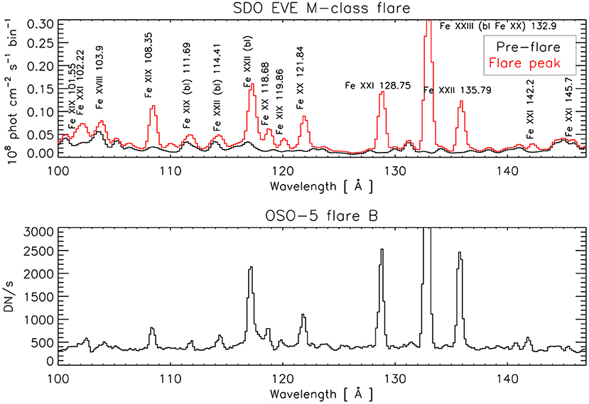
Figure 2. SDO EVE SXR spectra of an M-class flare (top), and the OSO-5 flare B spectrum by Kastner et al. (1974). Note that the OSO-5 spectrum is uncalibrated.

The SXR also provide excellent electron density diagnostics around 10¹¹ cm⁻³ of high-T plasma, as discussed by e.g., Mason et al. (1984). The EVE medium (1 Å) resolution made electron density measurements achievable although difficult, as discussed, e.g., by Milligan et al. (2012), Del Zanna and Woods (2013), and Keenan et al. (2017). OSO-5 and EVE measurements indicate densities of solar flares in the range 10^11.5–10¹² cm⁻³, as reviewed in Del Zanna and Mason (2018). However, spatially resolved measurements of such a fundamental parameter obtained from high-T spectral lines have been lacking.

As with the X-rays, the SXR allow line to continuum measurements, i.e., diagnostics of absolute chemical abundances (relative to hydrogen) of hot plasma during flares, as shown, e.g., by Warren (2014) using EVE spectra of large flares. Such measurements are in principle also available in the UV (Feldman et al., 2003).

The SXR contain lines from dozens of ions formed from 0.1 to 12 MK, plus all Iron ionization stages from Fe VIII to Fe XXIII. There are many diagnostics for the lower temperatures that are not discussed here, since this is not the focus of the paper. Covering temperatures from 0.1 to 12 MK in such a narrow region is a significant advantage over the other spectral ranges. We made a significant effort to review all the SXR lines taking into account a revision of available observations, to indicate which hot lines are likely to be blended with cooler lines. The main results are summarized in the Supplementary Material.

The identifications and atomic data for the cooler ions in the SXR still require a significant effort. We note that the strongest solar iron lines in the SXR were only identified recently by Del Zanna (2012) when benchmarking against laboratory and solar data a series of large-scale scattering calculations for the SXR. The new atomic data and identifications were introduced in CHIANTI version 8 by Del Zanna et al. (2015), but a large fraction of weaker lines still await firm identifications. Renewed efforts on measurements of laboratory plasma, such as those of Träbert et al. (2014) and on further atomic calculations should enable us to improve the completeness of the atomic data.

Doppler shifts of about 5 km s⁻¹ can easily be measured in the SXR, and large broadenings are relatively easy to measure in the against the background of cooler lines (which typically retain their small widths).

The first solar observations of the SXR range with an imaging spectrograph will be the upcoming flight of the Extreme Ultraviolet Normal Incidence Spectrograph (EUNIS). EUNIS will cover the wavelength range 92–112 Å employing a dual multilayer PdB₄C stack with two reflectivity peaks (of about 0.1) centered on the Fe XVIII 94 Å and Fe XIX 108 Å lines, and a few Å wide. Note that multilayer coatings designed specifically to target a few hot lines can provide higher reflectivities, such as proposed for the Multi-slit Solar Explorer (MUSE) and in this paper. MUSE, described in De Pontieu et al. (2020), is designed to observe the SXR Fe XIX 108.36 Å and Fe XXI 108.12Å lines (in addition to the strong coronal lines from Fe IX 171 and Fe XV 284 Å) with a large FOV (170′′ × 170′′) and a high resolution (0.4′′). The innovative and multiplexing design of this instrument will allow high cadence (12s) spectral observations in these four lines through the use of 37 slits (each spaced about 4.5′′ apart) covering a region of 170′′ × 170′′.

It is important to note that high spatial resolution can be achieved in the SXR with normal incidence. This has been shown by the two SXR channels of the SDO AIA (Lemen et al., 2012) telescopes, at 94 and 131 Å. Their sensitivity is high, due to good peak reflectances of the SXR multilayers (0.4 and 0.7, respectively, see Soufli et al., 2005), although obtained at the expense of narrow spectral bands. An additional advantage of the SXR is that the Zr front filters, employed for AIA for the first time in space, have shown minimal in-flight degradation (see e.g., Boerner et al., 2014), unlike nearly every filter adopted for EUV/UV instruments flown in space (see e.g., BenMoussa et al., 2013; Del Zanna and Mason, 2018). The main limitation of the SXR for a spectrometer has been the lack of multilayers with sufficiently high reflectances and wide spectral bands. A significant improvement has recently been obtained by Corso et al. (2021)² with multilayers of higher reflectances (0.25–0.4) at the specific wavelengths of the primary lines selected here.

3.3. EUV

The EUV has excellent diagnostics for lower-temperature plasma, up to about 4 MK, but there are only few “hot” lines. For example, the Hinode EIS instrument has provided excellent EUV observations of 1–4 MK plasma, but is “blind” until the very hot (about 15 MK) flare lines from Fe XXIII and Fe XXIV are observed (see e.g., Winebarger et al., 2012). These lines, as well as the low-temperature Fe XVII and Ca XVII lines require careful deblending from cooler lines, when their intensity is weak (see e.g., Young et al., 2007; Del Zanna, 2008; Warren et al., 2008; Del Zanna and Ishikawa, 2009; Del Zanna et al., 2011).

Within the EUV, there is also the strong Ca XVIII 302.2 Å line, observed by e.g., Skylab NRL-SO82A (see e.g., Dere, 1978) and the SPIRIT slitless spectroheliograph on board CORONAS-F (Shestov et al., 2014). Another important hot line in the EUV is the Fe XIX 592.2 Å line, which was first observed by the Skylab Harvard SO55 instrument, then by SoHO CDS, and more recently by the EUNIS-13 rocket flight (Brosius et al., 2014).

Currently, one advantage of the EUV over the X-rays is that high spatial resolution can be achieved with normal incidence, as shown, e.g., with the Hi-C sounding rocket, which obtained a spatial resolution of about 0.25′′(Kobayashi et al., 2014). Even higher resolutions are achievable in the UV, as e.g., shown by IRIS.

3.4. UV

The main UV hot lines are Fe XIX 1118.1 Å, Fe XX 721.5 Å, and Fe XXI 1354.1 Å. Several flare observations have been obtained with high-resolution imaging spectroscopy from e.g., SoHO SUMER (mostly of Fe XIX and Fe XXI) and IRIS (Fe XXI) (see e.g., Kliem et al., 2002; Polito et al., 2015). Fe XXI was also observed earlier by SMM/UVSP. The Fe XVIII 974 Å is another strong line, which was observed by SUMER (see e.g., Teriaca et al., 2012b), and is available to Solar Orbiter SPICE (Anderson et al., 2019). However, as we have mentioned, Fe XVIII has a significant contribution from 3 to 4 MK emission and so its use for measuring high temperatures by itself is limited.

A significant improvement in terms of sensitivity and resolution over SUMER is the EUV Spectroscopic Telescope (EUVST, see Shimizu et al., 2019), an M-class mission recently selected by the Japanese Space Agency (JAXA). The EUVST has a high throughput and a high spatial resolution of 0.4′′, with a design based on the LEMUR instrument (Teriaca et al., 2012a): the optical components have a standard Mo/Si ML for the EUV: 170–215 Å, and a B₄C top layer providing good reflectances in three UV bands: 690–850, 925–1,085, and 1,115–1,275 Å. The strongest lines in the wavelength regions 463–542 and 557–637 Å would be observed in second order.

EUVST has been designed to address a broad range of science questions. The key requirement for EUVST is to obtain high-cadence, high-resolution observations in spectral lines formed from photospheric to flare temperatures. It will also be able to provide observations of iron lines formed in the 5–10 MK range, hence will be able to provide important contributions to the science topics mentioned here. However, with the exception of Fe XIX, the lines from the other iron ions are intrinsically weaker than the resonance SXR lines, are observed in regions with lower sensitivities, and could be affected by photoabsorption in active regions. The planned EUVST spectral range is also limited in electron density diagnostics (see below). On the other hand, EUVST is excellent for measuring non-thermal widths and Doppler flows of a few km s⁻¹ (as it also has photospheric lines to measure rest wavelengths).

3.5. Density Diagnostics for Hot (10 MK) Plasma

Finally, a few comments about the important issue of measuring electron densities from line ratios. There are plenty of diagnostics and measurements across different temperatures, as summarized in the review by Del Zanna and Mason (2018), but very few for hot (10 MK) plasma. We provide here a summary and further details on the hot plasma diagnostics, which were not all included in the review. There are measurements with SMM FCS from Fe XXI, Fe XXII lines in the X-rays around 9 Å(Phillips et al., 1996), which indicated densities of 10¹³ cm⁻³ during a flare. These lines are very weak and are difficult to measure though. Still within the X-rays, there are potentially a few density diagnostic ratios from Fe XIX, Fe XXI, and Fe XXII, but these involve weak and often blended lines in a spectral region that is over-crowded even for the best crystal spectrometers, such as SMM FCS or the P78-1 SOLEX (McKenzie et al., 1980). Other density diagnostics involving satellite lines are available, but at wavelengths shorter than 2 Å. The He-like hot ions in the X-rays do provide density diagnostics, but only for densities above 10¹³ cm⁻³. At lower temperatures around 4 MK, Ne He-like lines have indicated densities of 10¹² cm⁻³ at the start of a flare (Wolfson et al., 1983).

Aside from the X-rays, the only other measurements of densities of hot plasma are those in the SXR, from OSO-5 (Mason et al., 1979; Mason et al., 1984) and EVE. These density diagnostics are well-known and well-studied in laboratory plasma (see e.g., Stratton et al., 1984). The atomic data and identifications for these n = 2 → n=2 transitions are well established. The best diagnostic ratios are those with the Fe XXI 102.2, 121.2, 142.2, 145.7 Å lines vs. the resonance line at 128.75 Å, as shown in Figure 3 (see also Table 1). They provide excellent measurements at relatively low densities, above 10¹⁰ cm⁻³. Other ratios involve Fe XIX, Fe XX, and Fe XXII lines. There are also interesting ratios involving Fe XIX lines, as shown in Figure 3: they are sensitive to very low densities, between 10⁸ and 10¹⁰ cm⁻³, which would be particularly important to investigate further. The variation in the Fe XIX ratios is only 25% but measurable, especially if the multi-layers are fine-tuned to increase the signal in the weaker density-sensitive lines. It would therefore be possible to measure any densities from 10⁸ to 10¹³ cm⁻³ and above, observing both the Fe XIX and Fe XXI line ratios. That would be quite an achievement.

FIGURE 3

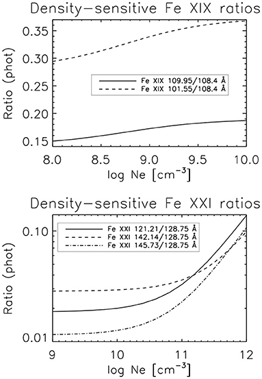
Figure 3. A few of the available SXR density-sensitive ratios.

There are in principle other density diagnostics at longer wavelengths. Within the EUV, a good density diagnostic above 10¹² cm⁻³ available at the EUVST wavelengths is the Fe XX 567.8/721.5 Å ratio, although it could be affected by neutral hydrogen absorption in active region observations. The 567.8 Å is intrinsically a relatively strong line, but will be observed in second order, where the sensitivity is low. Also, as the thermal width at 10 MK of the 567.8 line is 0.17 Å, the line will be blended with the strong Si VII 1135.4 Å transition.

There are also two other options outside the EUVST spectral range. One is the Fe XXI 786/1354 Å ratio, useful for densities higher than 10¹¹ cm⁻³. The other one, Fe XIX 1,328/1,118 Å, is an excellent diagnostic for densities of 10¹¹ cm⁻³ or lower (see e.g., Feldman et al., 2000), although the 1,328 Å line is intrinsically very weak: at 10¹⁰ cm⁻³, its intensity is only 2% that of the 1,118 Å line, and decreases with density.

4. Observed and Predicted Count Rates in the SXR

4.1. Straw-Man Design

To illustrate the current capability for an imaging SXR spectrograph, an example (straw-man) instrument is presented. For high collecting area and resolution, the telescope mirror is a 20 cm diameter off-axis paraboloid with a focal length of 2 m that feeds a spectrograph with a magnification of 1.4, along the lines of the successful Hinode EIS. A back-illuminated CCD (or CMOS array) with 13.5 μm pixels at a distance of 1.4 m from the grating provides an image scale of 1′′/pixel. Reducing the spatial resolution from e.g., the 0.3′′ of the original LEMUR design not only increases the throughput but also significantly simplifies the thermal requirements for a more compact instrument. Clearly, a higher spatial resolution would be desirable, but would have to be evaluated in a trade-off study, to ensure that, depending on the size of the primary, sufficient signal can be obtained to achieve the science goals of a specific mission.

In a recent study, Corso et al. (2021)² produced a few new multilayers (ML), tuned to have peak reflectances in our primary SXR lines. We adopt two MLs: a 3-fold Mo/Si standard ML for the 126–150 Å range, and a new aperiodic B₄C/Y/B₄C/Pd for the 100–126 Å range. As the SXR hot primary lines cannot be observed with a single multilayer, we envisage that both the mirror and the grating would be segmented in two halves, each with a separate ML, as in the EIS instrument.

The spectral dispersion can be chosen to use one or two 2,048 × 2,048 pixel detectors to cover the wavelength region of interest. Holographic gratings with excellent micro-roughness on the scales relevant to obtaining high SXR reflectivity (0.3 nm on spatial scales of 0.01–1 um) have been demonstrated with line densities of 4,000/mm and a blaze to maximize throughput (the EUNIS flight grating has a density of 3,800 l/mm, the EIS one 4,200 l/mm). If used in first or second order, this would provide a dispersion of 12 or 24 mÅ/pixel and a wavelength range of 24 or 49 Å per detector, respectively. At the Nyquist limit, that provides a resolving power of R = 2,500 in first order (comparable to previous EUV spectrographs), or R = 5,000 in second order. We select the second option here, and use the grating efficiencies in second order calculated by Corso et al. (2021)², which are close to 40%. The second order with two 2,048 pixel detectors (as the Hinode EIS) provides a pixel size of 0.01 Å, corresponding to about 20 km s⁻¹. This means that Dopplershifts of 2–5 km s⁻¹ are measurable. We note that reconnection and associated flows are expected to be very fast (on short time scales) so even a resolution of a few tens of km s⁻¹ for the hot lines could be sufficient.

With a 0.01 Å slit, a 0.03 Å (or better) spectral resolution is achievable. The thermal FWHM of the Fe ions in the ranges 6–10 MK and 108–135 Å is 0.025–0.04 Å, so with such resolution the thermal width would be resolved. However, considering that significant non-thermal widths in the hot lines are likely present, a lower spectral resolution could be sufficient. In the plots that follow, we have adopted a 0.01 Å pixel resolution, included a thermal width of the lines (using their peak formation temperature), and added an instrumental FWHM of 0.025 Å.

An alternative option would be a 4,000/mm grating in first order, which would have higher efficiency (better than 50%) and would reduce the spectrograph size by 80%, at the expense of a 0.02 Å pixel resolution, which would still be acceptable.

For the detector, we have assumed an efficiency of 0.8, achievable with standard CCDs, such as the 4kx4k thinned back-illuminated CCDs used by AIA. We note that these CCDs have been proven very stable and higher efficiencies (0.85) have been achieved (Hi-C).

We have included a front filter, the same one used for the AIA 94 and 131 Å channels: a Zr filter, which has a transmission across the soft X-rays of about 0.4. We note that such filter includes a reduction of 15% due to the supporting mesh, although a mesh with a 95% transmission has been flown aboard Hi-C (see e.g., Kobayashi et al., 2014), so better transmission is achievable. We also note that the inclusion of a safety redundant filter in front of the detector would reduce by about 50% the signal we predict here. An alternative, adopted for the EUNIS-13 flight, would be not to use a front filter and use a KBr coated micro-channel plate (MCP) detector (not affected by visible light) instead of a CCD detector. In this case, the detected signal would be much higher than the values presented here.

Figure 4 shows the resulting effective area, which is the product of the filter transmission, the reflectivity of the primary, that of the grating, the grating efficiency, the geometrical area and the quantum efficiency of the detector. For comparison purposes, the same figure also shows the LEMUR (Teriaca et al., 2012a) effective area in the EUV and UV, scaled to the same geometrical area of each SXR channel. The figure clearly indicates that similar effective areas are achievable in the SXR and UV, for an equivalent aperture. As we have seen that the photons emitted by the hot lines in the SXR and UV are comparable, this indicates that similar numbers of detected photons are achievable either in the SXR or the UV. We note however that the EUVST baseline design assumes a large primary mirror with a 28 cm diameter, so its effective area is actually about a factor of four higher than what is shown in the EUV and UV panels in Figure 4. We also note that MUSE has a comparable effective area of 2 cm², while MaGIXS has a peak effective area of 0.03 cm² (Athiray et al., 2019).

FIGURE 4

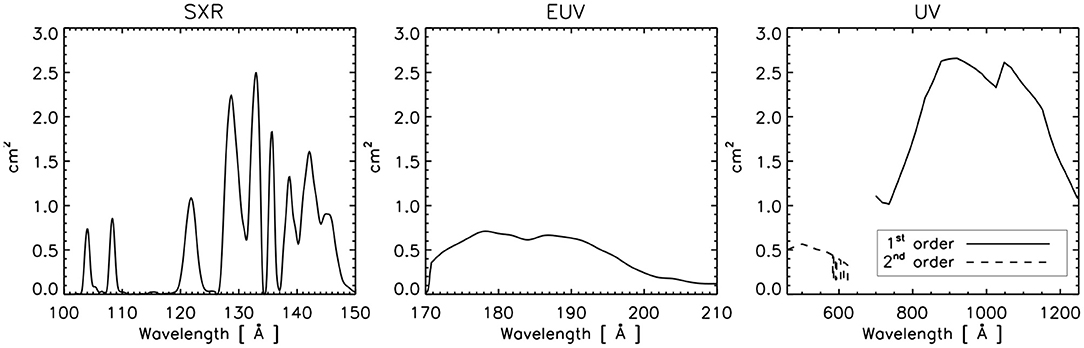
Figure 4. Effective areas for the soft X-ray channels (left), with those of a scaled-down version of the LEMUR instrument in the EUV/UV (see text).

To estimate the signal S detected (data numbers per second, DN/s) in a pixel we use:

$\begin{array}{ll}S=I_{\text{r}}{A}_{\text{eff}}\frac{12398.5}{3.65\lambda G}\Omega & (1)\end{array}$

where the terms convert the number of electrons produced in the CCD by a photon of wavelength λ (Å) into data numbers DN. I_r is the incident radiance, A_eff is the effective area, G is the gain of the camera, and Ω is the solid angle subtended by a pixel. We have assumed a gain of 6.3, the same as the EIS CCD.

4.2. Count Rates for the 10 MK Emission

We now return to the 10 MK simulation. The first radiance column in Table 1 shows that the Fe XIX 1118.0 Å radiance is 0.23 erg cm⁻² s⁻¹ sr⁻¹, which is very close to the minimum values (0.22–0.5) recorded (with a total exposure of 2 h and only in some locations) by SUMER (Parenti et al., 2017).

The Fe XIX 592.2 Å radiance is 0.24 erg cm⁻² s⁻¹ sr⁻¹, a value over 20 times lower than that measured with EUNIS-13 by Brosius et al. (2014), but not inconsistent with other EUNIS-13 observations, as we have mentioned.

Figure 5 shows the expected SXR count rates for the very weak 10 MK emission of Figure 1. The 10 MK spectrum has been added to that of an active region core, discussed in the Supplementary Material. Note that the units in the spectra are per pixel (0.01 Å) resolution, while Table 1 provides the total count rates in the lines.

FIGURE 5

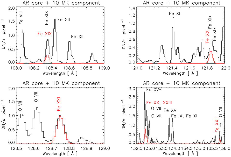
Figure 5. Simulated count rates (1′′ pixel) for the emission from a very weak isothermal plasma at 10 MK (red spectrum), added to the emission from a quiescent active region core (black spectrum).

As we have discussed, a good proxy for the 5–10 MK emission are Fe XIX and higher ionization stages. The count rates in the Fe XIX– Fe XXIII strongest lines are in the range 1.4–6.5. Such signals are easily measurable with a cadence of a few seconds and spatial averaging over ≃4′′. This is a major improvement over the 2 h exposures and spatial averaging obtained with SUMER in Fe XIX (Parenti et al., 2017).

As we have mentioned, none of the previous observations of hot emission in AR quiescent cores were able to provide an indication of the distribution of temperatures above 5 MK. Upper limits in the 4–15 MK range have been provided by continuum emission or the Mg XII images. The few Fe XIX observations from SUMER and CDS provide a similarly unclear picture. So it is possible that the count rates we estimate at 10 MK are either an over- or an under-estimate by a large margin. If say they were over-estimated by two orders of magnitude, a measureable signal of ≃100 DN/s could be obtained by an acceptable spatial averaging over ≃20′′ and a 2-min exposure.

The Fe XIX 108.36 Å, Fe XX 121.85 Å, Fe XXI 128.75 Å, and Fe XXII 135.81 Å resonance lines are all excellent candidates. The Fe XIX 108.36 Å has a small contribution from the quiescent AR core, which is questionable. The Fe XX 121.85 Å is super-imposed on an unidentified weak Fe XI transition which is currently expected at the same wavelength, although the quiet Sun spectra suggest that this is not the case (see the Supplementary Material). As there are many Fe XI transitions within the two SXR channels, it would be easy to deblend the Fe XI contribution, if the line was at that wavelength.

The Fe XXI 128.75 Å is unblended, while the Fe XXII 135.81 Å is blended on its red wing with a O VII 135.83 Å line. The O VII can accurately be estimated measuring other O VII transitions, such as the strong O VII 120.33 Å self-blend. Finally, the Fe XXIII could be deblended from the O VII and other lines.

4.3. Count Rates From a Nanoflare Simulation

To provide an estimate based on a numerical nanoflare simulation, we took the DEM distribution from the L = 120 Mm case as described by López Fuentes and Klimchuk (2015). This simulation is realistic in that it includes a variety of magnitudes and frequencies. The DEM distribution has large values at low temperatures, hence the simulation also naturally includes all the transition-region lines, as well as the coronal and the hot lines. As we would expect low densities around 10⁸ cm⁻³ for the hotter plasma and higher ones (10⁹ cm⁻³) for the coronal lines, we have adopted a constant pressure of 10^15.5 cm⁻³ K for the simulated spectra. Figure 6 and Table 1 show the expected SXR count rates. There is clearly a very strong signal in all the hot primary lines (i.e., from Fe XVIII–Fe XXIII).

FIGURE 6

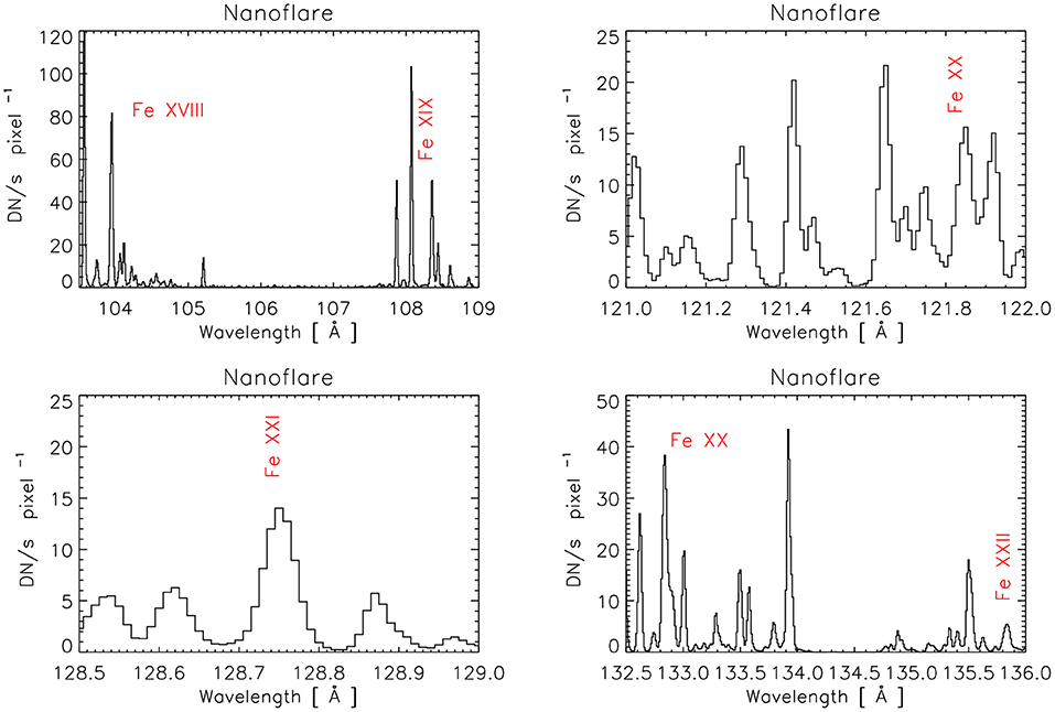
Figure 6. Simulated count rates (1′′ pixel) for the emission from a nanoflare simulation (López Fuentes and Klimchuk, 2015). The main hot lines are labeled.

4.4. Count Rates for a Sub-A Class Microflare, Additional Broadening and Densities

To estimate the signal for a very weak microflare, we consider the 0.005 A-class NuSTAR observations discussed by Cooper et al. (2020). The NuSTAR X-ray Bremsstrahlung emission was well fitted with an isothermal emission of 6.7 MK. The signal in the AIA 94 Å band, due to Fe XVIII, was at the limit of detection. We converted the volume EM to a column emission measure EM = 1.18 × 10²⁷ (cm⁻⁵). Using our “coronal” abundances we expect about 3 DN/s/pixel due to Fe XVIII in the AIA 94 Å band, close to what was observed. Figure 7 shows sections of our predicted SXR count rates for a density of 10¹¹ cm⁻³, added to those of the active region core discussed in the Supplementary Material. The total count rates are given in Table 1.

FIGURE 7

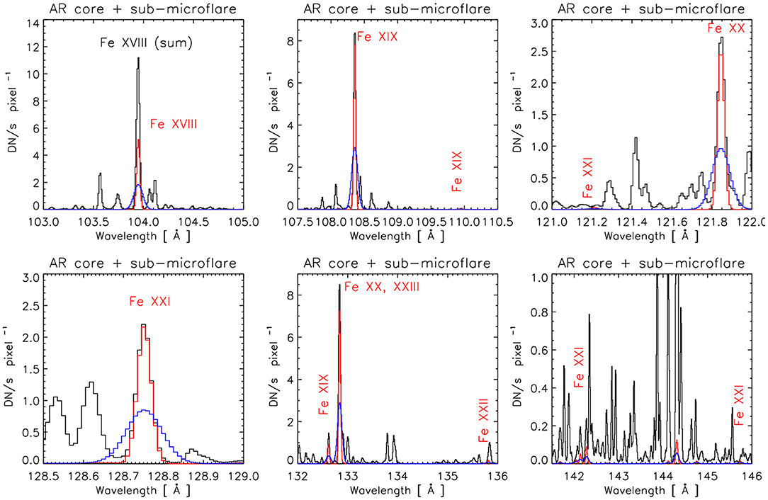
Figure 7. Simulated SXR count rates (1′′ pixel) for a sub-A class microflare of 6.7 MK (red spectrum). The black spectrum is the sum of the microflare and active region core. The blue spectrum shows the hot emission from the sub-A class microflare but with an additional broadening of 200 km s⁻¹ FWHM.

There is plenty of signal in all the resonance lines. They are not affected by the “background” emission, with the exception of Fe XXII, which is very weak given such a low temperature, and Fe XVIII, as significant quiescent emission is expected to be present. Time-dependent ionization on a 1′′ spatial scale could be studied with exposure times of 1–10s.

The figure also shows the effect of an additional broadening of 200 km s⁻¹ FWHM, which would be easily measurable for the main Fe XVIII, Fe XIX, Fe XX, and Fe XXI lines, as no significant background emission from cooler lines is present. Much stronger broadenings would become difficult to observe, for this very weak hot emission.

Regarding density measurements, the comparisons with irradiance spectra shown in the Supplementary Material indicate that the Fe XIX 119.98 Å and Fe XXI 121.21, 142.2 Å density-sensitive lines fall in regions relatively free of background emission. The Fe XXI 145.73 Å, on the other hand, is close to a Ni X line and would require background subtraction. The expected count rates indicate that even for this extremely weak microflare, densities could be measured with exposure times of about 100 s at 1′′ resolution.

4.5. Count Rates for an A Class Microflare

As representative of a weak A class microflare, we have considered an isothermal plasma emission at 8 MK, an electron density of N_e = 10¹¹ cm⁻³, the Del Zanna (2013) coronal abundances and an emission measure EM = 10²⁹ cm⁻⁵. The microflare radiances are listed in Table 1. These parameters were chosen so as to reproduce the Fe XVII and Ca XVII radiances during the peak emission of a microflare recorded by EIS (Mitra-Kraev and Del Zanna, 2019). We note that the actual peak temperature of the post-flare loops was about 5 MK, although short-lived higher temperatures were probably present during the impulsive phase in one of the footpoints (see also Testa and Reale, 2020). Using the effective areas of the instruments, we found out that such a weak 8 MK microflare would be invisible to EIS in Fe XXIII and at the limit of detection for IRIS in the Fe XXI 1354.1 Å line (we estimate 3 IRIS DN/s in the line). On the other hand, it would have been well observed by the SDO AIA SXR bands, with about 200 DN/s in the Fe XVIII 94 Å channel and 126 DN/s in Fe XXI within the 131 Å band.

Figure 8 shows the simulated SXR count rates (1′′ pixel) for the microflare case study, added to those of the active region core discussed in the Supplementary Material. The SXR channel provides very large count rates in all the primary lines, as listed in Table 1. For example, the Fe XXI 128.75 Å resonance line would produce 3.0 × 10³ DN/s. The Fe XIX and Fe XXI density-sensitive lines are also strong, providing excellent density measurements with very short timescales of a second or so at 1′′ resolution. Larger (e.g., B-class) flares would require sub-second exposure times to avoid saturation.

FIGURE 8

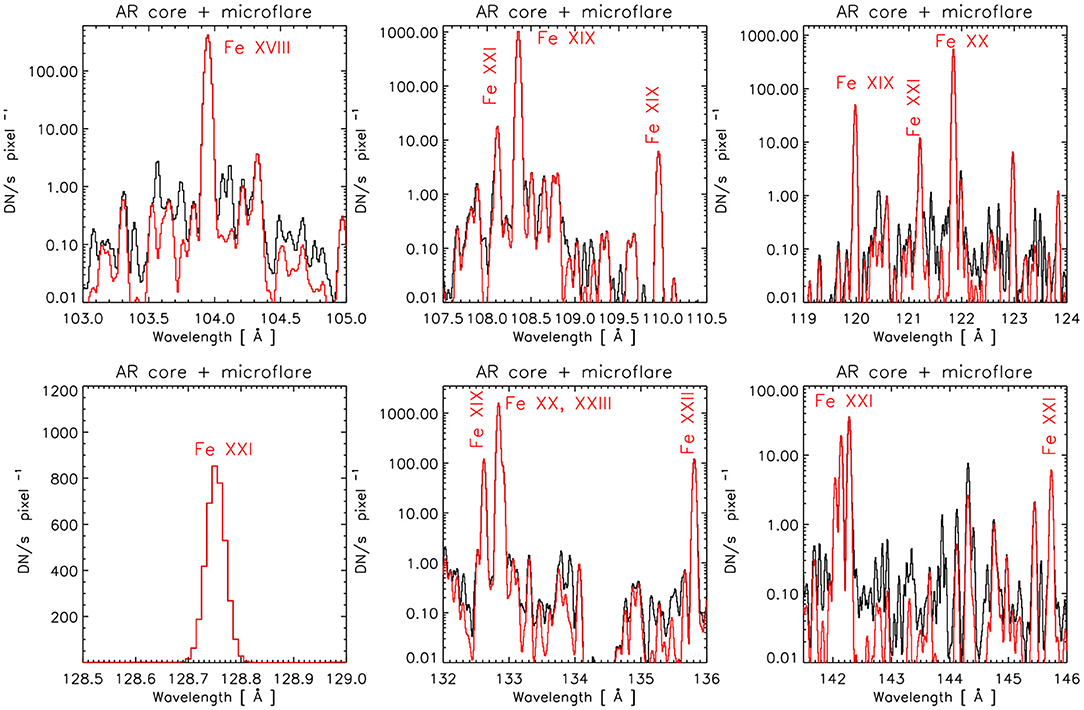
Figure 8. Simulated SXR count rates (1′′ pixel) for an 8 MK A-class microflare (red spectrum), added to those of an active region core. The black spectrum is the sum of the two.

The significant differences with the spectra of the sub-A class microflare are due not just to the increased emission measure, but also to the increased temperature, from 6.7 to 8 MK.

5. Conclusions

Understanding a range of heating/cooling events in active regions and probing for the presence of time-dependent ionization requires high-resolution line spectroscopy of 5–10 MK plasma, with observations of multiple ionization stages of an element and simultaneous observations of the electron densities. This has never been achieved in solar physics. There are plenty of detailed observations of cooler or hotter plasma, but very few around these temperatures.

In this paper, we have demonstrated that the soft X-ray around 100 Å is the best range to carry out such investigations, since it provides, in a relatively narrow wavelength range of ~50 Å, six ionization stages of iron to probe 5–10 MK plasma, together with excellent density diagnostics above 10¹⁰ cm⁻³, plus some above 10⁸ cm⁻³. As this spectral region is practically unexplored, we have provided here and in the Supplementary Material an overview of the main spectral features for different solar conditions, from the quiet Sun to active regions, nanoflares and microflares. The primary SXR hot lines are very strong, close in wavelength and very sensitive to temperatures in the 5–12 MK range.

We have presented estimated count rates with a straw-man imaging spectrometer, similar in size to the successful Hinode EIS instrument. The technology for a soft X-ray instrument is mature. With the exception of the new multilayers, which would have to be fabricated and tested, all the components are standard, have flown on previous missions, and have proven to be long-lived. However, as discussed in Corso et al. (2021)², multilayers of the type adopted here have already been fabricated and have shown good stability to thermal effects and over time (see e.g., Windt and Gullikson, 2015).

We have shown that effective areas comparable to those in the UV (for equivalent telescope aperture) can be achieved with high spatial resolutions of 1′′ or better. Time-dependent ionization, heating and cooling cycles can be studied at such resolutions with a cadence of seconds for a wide range of sub A-class microflares. Flows can be studied with a few km s⁻¹ resolutions. The unresolved hot emission expected to result from nanoflares can be studied with a cadence of a few seconds with spatial averaging.

The present concept for a SXR spectrometer is designed to demonstrate the potential for discovery in that largely unexplored wavelength range, with the primary science goal of understanding the physics of the hot (5-10 MK) plasma in active regions. As such, this straw-man instrument is complementary to other future or proposed missions designed to address, for instance, the top-level science objective of the formation mechanisms of the hot and dynamic outer solar atmosphere, as described in the report of the Next Generation Solar Physics Mission Science Objectives Team, NGSPM-SOT.

Once the first SXR observations from EUNIS and further laboratory observations become available, it will be possible to confirm the present predictions, thus allowing to perform trade-off studies for specific science goals. In particular, the multi-layers adopted here were designed to maximize the signal in the primary resonance lines in the six ionization stages of iron, but could be adjusted to increase the signal in the much weaker density-sensitive lines. Also, a scaled-down version of the proposed straw-man design would result in a very compact and cost-effective instrument, producing novel observations in this unexplored region.

In summary, the 5–10 MK temperature regime is a largely unexplored discovery space, precisely where magnetic energy conversion is occurring. High-resolution spectroscopy in this regime can be expected to provide breakthroughs. Although in this paper we have focused on the almost unexplored 5–10 MK plasma emission, the SXR instrument is also sensitive to a broad range of temperatures, from 0.1 to 5 MK, with many diagnostics not discussed here. Also, the proposed SXR instrument is sensitive to larger (B-class and over) flares and higher temperatures, up to around 15–20 MK with Fe XXIII and even higher with the continuum emission, with timescales much shorter than a second.

Data Availability Statement

The original contributions presented in the study are included in the article/Supplementary Material, further inquiries can be directed to the corresponding author/s.

Author Contributions

GD wrote the article and produced the figures but received contributions to the text from all the co-authors. AC also provided the reflectivities of the multilayers and the grating. AD (PI of EUNIS-13) also contributed to the figures for the straw-man design. JK also provided the results of the nanoflare simulations. All authors contributed to the article and approved the submitted version.

Funding

GD and HM acknowledge support from STFC (UK) via the consolidated grants to the atomic astrophysics group (AAG) at DAMTP, University of Cambridge (ST/P000665/1 and ST/T000481/1). The work of JK was supported by the GSFC Internal Scientist Funding Model (competitive work package) program. AD acknowledges support through NASA Heliophysics awards 13-HTIDS13 2-0074 and 16-HTIDS16_2-0064.

Conflict of Interest

The authors declare that the research was conducted in the absence of any commercial or financial relationships that could be construed as a potential conflict of interest.

Acknowledgments

We would like to thank Bart De Pontieu (USA), Vanessa Polito (USA), and Luca Teriaca (Germany) for providing useful comments on the manuscript, as well as the reviewers.

Supplementary Material

The Supplementary Material for this article can be found online at: https://www.frontiersin.org/articles/10.3389/fspas.2021.638489/full#supplementary-material

The Supplementary Material presents an analysis of quiet Sun SXR spectra, and predicted spectra for the quiet Sun and quiescent active region cores, to show the expected “background” emission.

Footnotes

1. ^Vadawale, S. V., Mondal, B., Mithun, N. P. S., (2021). Observations of the Quiet Sun During the Deepest Solar Minimum of the Past Century with Chandrayaan-2 XSM. Astrophys. J.

2. ^Corso, A., Del Zanna, G., and Polito, V. (2021). Future perspectives in solar hot plasma observations in the soft X-rays. Exp. Astron.

References

Acton, L. W., Finch, M. L., Gilbreth, C. W., Culhane, J. L., Bentley, R. D., Bowles, J. A., et al. (1980). The soft X-ray polychromator for the solar maximum mission. Sol. Phys. 65, 53–71. doi: 10.1007/BF00151384

CrossRef Full Text | Google Scholar

Anderson, M., Appourchaux, T., Auchère, F., Aznar Cuadrado, R., Barbay, J., Baudin, F., et al. (2019). The solar orbiter SPICE instrument–an extreme UV imaging spectrometer. Astron. Astrophys. 642:A14. doi: 10.1051/0004-6361/201935574

CrossRef Full Text | Google Scholar

Athiray, P. S., Vievering, J., Glesener, L., Ishikawa, S.-n., Narukage, N., Buitrago-Casas, J. C., et al. (2020). FOXSI-2 solar microflares. I. Multi-instrument differential emission measure analysis and thermal energies. Astrophys. J. 891:78. doi: 10.3847/1538-4357/ab7200

CrossRef Full Text | Google Scholar

Athiray, P. S., Winebarger, A. R., Barnes, W. T., Bradshaw, S. J., Savage, S., Warren, H. P., et al. (2019). Solar active region heating diagnostics from high-temperature emission using the MaGIXS. Astrophys. J. 884:24. doi: 10.3847/1538-4357/ab3eb4

CrossRef Full Text | Google Scholar

Barnes, W. T., Cargill, P. J., and Bradshaw, S. J. (2016a). Inference of heating properties from “hot” non-flaring plasmas in active region cores. I. Single nanoflares. Astrophys. J. 829:31. doi: 10.3847/0004-637X/829/1/31

CrossRef Full Text | Google Scholar

Barnes, W. T., Cargill, P. J., and Bradshaw, S. J. (2016b). Inference of heating properties from “hot” non-flaring plasmas in active region cores. II. Nanoflare trains. Astrophys. J. 833:217. doi: 10.3847/1538-4357/833/2/217

CrossRef Full Text | Google Scholar

BenMoussa, A., Gissot, S., Schühle, U., Del Zanna, G., Auchère, F., Mekaoui, S., et al. (2013). On-orbit degradation of solar instruments. Sol. Phys. 288, 389–434. doi: 10.1007/s11207-013-0290-z

CrossRef Full Text | Google Scholar

Benz, A. O. (2017). Flare observations. Liv. Rev. Sol. Phys. 14:2. doi: 10.1007/s41116-016-0004-3

CrossRef Full Text | Google Scholar

Boerner, P. F., Testa, P., Warren, H., Weber, M. A., and Schrijver, C. J. (2014). Photometric and thermal cross-calibration of solar EUV instruments. Sol. Phys. 289, 2377–2397. doi: 10.1007/s11207-013-0452-z

CrossRef Full Text | Google Scholar

Bradshaw, S. J., and Cargill, P. J. (2006). Explosive heating of low-density coronal plasma. Astron. Astrophys. 458, 987–995. doi: 10.1051/0004-6361:20065691

CrossRef Full Text | Google Scholar

Bradshaw, S. J., and Mason, H. E. (2003). A self-consistent treatment of radiation in coronal loop modelling. Astron. Astrophys. 401, 699–709. doi: 10.1051/0004-6361:20030089

CrossRef Full Text | Google Scholar

Brosius, J. W. (2003). Chromospheric evaporation and warm rain during a solar flare observed in high time resolution with the coronal diagnostic spectrometer aboard the solar and heliospheric observatory. Astrophys. J. 586, 1417–1429. doi: 10.1086/367958

CrossRef Full Text | Google Scholar

Brosius, J. W. (2013). Chromospheric evaporation in solar flare loop strands observed with the extreme-ultraviolet imaging spectrometer on board Hinode. Astrophys. J. 762:133. doi: 10.1088/0004-637X/762/2/133

CrossRef Full Text | Google Scholar

Brosius, J. W., and Daw, A. N. (2015). Quasi-periodic fluctuations and chromospheric evaporation in a solar flare ribbon observed by IRIS. Astrophys. J. 810:45. doi: 10.1088/0004-637X/810/1/45

CrossRef Full Text | Google Scholar

Brosius, J. W., Daw, A. N., and Rabin, D. M. (2014). Pervasive faint Fe XIX emission from a solar active region observed with EUNIS-13: evidence for nanoflare heating. Astrophys. J. 790:112. doi: 10.1088/0004-637X/790/2/112

CrossRef Full Text | Google Scholar

Cargill, P. J. (1994). Some implications of the nanoflare concept. Astrophys. J. 422, 381–393. doi: 10.1086/173733

CrossRef Full Text | Google Scholar

Cargill, P. J. (2014). Active region emission measure distributions and implications for nanoflare heating. Astrophys. J. 784:49. doi: 10.1088/0004-637X/784/1/49

CrossRef Full Text | Google Scholar

Cargill, P. J., and Klimchuk, J. A. (2004). Nanoflare heating of the corona revisited. Astrophys. J. 605, 911–920. doi: 10.1086/382526

CrossRef Full Text | Google Scholar

Caspi, A., Woods, T. N., and Warren, H. P. (2015). New observations of the solar 0.5–5 keV soft X-ray spectrum. Astrophys. J. Lett. 802:L2. doi: 10.1088/2041-8205/802/1/L2

CrossRef Full Text | Google Scholar

Cooper, K., Hannah, I. G., Grefenstette, B. W., Glesener, L., Krucker, S., Hudson, H. S., et al. (2020). NuSTAR observation of a minuscule microflare in a solar active region. Astrophys. J. Lett. 893:L40. doi: 10.3847/2041-8213/ab873e

CrossRef Full Text | Google Scholar

Culhane, J. L., Harra, L. K., James, A. M., Al-Janabi, K., Bradley, L. J., Chaudry, R. A., et al. (2007). The EUV imaging spectrometer for Hinode. Sol. Phys. 243, 19–61. doi: 10.1007/s01007-007-0293-1

CrossRef Full Text | Google Scholar

De Pontieu, B., Martínez-Sykora, J., Testa, P., Winebarger, A. R., Daw, A., Hansteen, V., et al. (2020). The multi-slit approach to coronal spectroscopy with the multi-slit solar explorer (MUSE). Astrophys. J. 888:3. doi: 10.3847/1538-4357/ab5b03

CrossRef Full Text | Google Scholar

De Pontieu, B., Title, A. M., Lemen, J. R., Kushner, G. D., Akin, D. J., Allard, B., et al. (2014). The interface region imaging spectrograph (IRIS). Sol. Phys. 289, 2733–2779. doi: 10.1007/s11207-014-0485-y

PubMed Abstract | CrossRef Full Text | Google Scholar

Del Zanna, G. (1995). EUV Spectroscopy of Stellar Coronae. Ph.D. thesis, University of Florence, Florence, Italy.

Google Scholar

Del Zanna, G. (2008). Flare lines in Hinode EIS spectra. Astron. Astrophys. 481, L69–L72. doi: 10.1051/0004-6361:20079033

CrossRef Full Text | Google Scholar

Del Zanna, G. (2012). Benchmarking atomic data for astrophysics: a first look at the soft X-ray lines. Astron. Astrophys. 546:A97. doi: 10.1051/0004-6361/201219923

CrossRef Full Text | Google Scholar

Del Zanna, G. (2013). The multi-thermal emission in solar active regions. Astron. Astrophys. 558:A73. doi: 10.1051/0004-6361/201321653

CrossRef Full Text | Google Scholar

Del Zanna, G., Berlicki, A., Schmieder, B., and Mason, H. E. (2006). A multi-wavelength study of the compact M1 flare on October 22, 2002. Sol. Phys. 234, 95–113. doi: 10.1007/s11207-006-0016-6

CrossRef Full Text | Google Scholar

Del Zanna, G., Dere, K. P., Young, P. R., and Landi, E. (2020). CHIANTI–an atomic database for emission lines. Version 10. Astrophys. J. 909:38. doi: 10.3847/1538-4357/abd8ce

CrossRef Full Text | Google Scholar

Del Zanna, G., Dere, K. P., Young, P. R., Landi, E., and Mason, H. E. (2015). CHIANTI–an atomic database for emission lines. Version 8. Astron. Astrophys. 582:A56. doi: 10.1051/0004-6361/201526827

CrossRef Full Text | Google Scholar

Del Zanna, G., and Ishikawa, Y. (2009). Benchmarking atomic data for astrophysics: Fe XVII EUV lines. Astron. Astrophys. 508, 1517–1526. doi: 10.1051/0004-6361/200911729

CrossRef Full Text | Google Scholar

Del Zanna, G., and Mason, H. E. (2014). Elemental abundances and temperatures of quiescent solar active region cores from X-ray observations. Astron. Astrophys. 565:A14. doi: 10.1051/0004-6361/201423471

CrossRef Full Text | Google Scholar

Del Zanna, G., and Mason, H. E. (2018). Xuv spectroscopy. Liv. Rev. Sol. Phys. 15:5. doi: 10.1007/s41116-018-0015-3

CrossRef Full Text | Google Scholar

Del Zanna, G., Mitra-Kraev, U., Bradshaw, S. J., Mason, H. E., and Asai, A. (2011). The 22 May 2007 B-class flare: new insights from Hinode observations. Astron. Astrophys. 526:A1. doi: 10.1051/0004-6361/201014906

CrossRef Full Text | Google Scholar

Del Zanna, G., and Woods, T. N. (2013). Spectral diagnostics with the SDO EVE flare lines. Astron. Astrophys. 555:A59. doi: 10.1051/0004-6361/201220988

CrossRef Full Text | Google Scholar

Dere, K. P. (1978). Spectral lines observed in solar flares between 171 and 630 angstroms. Astrophys. J. 221, 1062–1067. doi: 10.1086/156110

CrossRef Full Text | Google Scholar

Dere, K. P., Landi, E., Mason, H. E., Monsignori Fossi, B. C., and Young, P. R. (1997). CHIANTI–an atomic database for emission lines. Astron. Astrophys. Suppl. 125, 149–173. doi: 10.1051/aas:1997368

CrossRef Full Text | Google Scholar

Dudík, J., Dzifčáková, E., Del Zanna, G., Mason, H. E., Golub, L. L., Winebarger, A. R., et al. (2019). Signatures of the non-Maxwellian κ-distributions in optically thin line spectra. II. Synthetic Fe XVII-XVIII X-ray coronal spectra and predictions for the Marshall Grazing-Incidence X-ray Spectrometer (MaGIXS). Astron. Astrophys. 626:A88. doi: 10.1051/0004-6361/201935285

CrossRef Full Text | Google Scholar

Dudík, J., Dzifčáková, E., Meyer-Vernet, N., Del Zanna, G., Young, P. R., Giunta, A., et al. (2017). Nonequilibrium processes in the solar corona, transition region, flares, and solar wind (invited review). Sol. Phys. 292:100. doi: 10.1007/s11207-017-1125-0

CrossRef Full Text | Google Scholar

Dudík, J., Janvier, M., Aulanier, G., Del Zanna, G., Karlický, M., Mason, H. E., et al. (2014). Slipping magnetic reconnection during an X-class solar flare observed by SDO/AIA. Astrophys. J. 784:144. doi: 10.1088/0004-637X/784/2/144

CrossRef Full Text | Google Scholar

Feldman, U., Curdt, W., Landi, E., and Wilhelm, K. (2000). Identification of spectral lines in the 500–1600 Åwavelength range of highly ionized Ne, Na, Mg, Ar, K, Ca, Ti, Cr, Mn, Fe, Co, and Ni emitted by flares (Te > 3 × 10⁶ K) and their potential use in plasma diagnostics. Astrophys. J. 544, 508–521. doi: 10.1086/317203

CrossRef Full Text | Google Scholar

Feldman, U., Doschek, G. A., Behring, W. E., and Phillips, K. J. H. (1996). Electron temperature, emission measure, and X-ray flux in A2 to X2 X-ray class solar flares. Astrophys. J. 460, 1034–1041. doi: 10.1086/177030

CrossRef Full Text | Google Scholar

Feldman, U., Landi, E., Doschek, G. A., Dammasch, I., and Curdt, W. (2003). Free-free emission in the far-ultraviolet spectral range: a resource for diagnosing solar and stellar flare plasmas. Astrophys. J. 593, 1226–1241. doi: 10.1086/376680

CrossRef Full Text | Google Scholar

Fletcher, L., Dennis, B. R., Hudson, H. S., Krucker, S., Phillips, K., Veronig, A., et al. (2011). An observational overview of solar flares. Space Sci. Rev. 159, 19–106. doi: 10.1007/978-1-4614-3073-5_3

CrossRef Full Text | Google Scholar

Fletcher, L., and Hudson, H. S. (2008). Impulsive phase flare energy transport by large-scale Alfvén waves and the electron acceleration problem. Astrophys. J. 675, 1645–1655. doi: 10.1086/527044

CrossRef Full Text | Google Scholar

Golub, L., Hartquist, T. W., and Quillen, A. C. (1989). Comments on the observability of coronal variations. Sol. Phys. 122, 245–261. doi: 10.1007/BF00912995

CrossRef Full Text | Google Scholar

Graham, D. R., and Cauzzi, G. (2015). Temporal evolution of multiple evaporating ribbon sources in a solar flare. Astrophys. J. Lett. 807:L22. doi: 10.1088/2041-8205/807/2/L22

CrossRef Full Text | Google Scholar

Hannah, I. G., Christe, S., Krucker, S., Hurford, G. J., Hudson, H. S., and Lin, R. P. (2008). RHESSI microflare statistics. II. X-ray imaging, spectroscopy, and energy distributions. Astrophys. J. 677, 704–718. doi: 10.1086/529012

CrossRef Full Text | Google Scholar

Hannah, I. G., Grefenstette, B. W., Smith, D. M., Glesener, L., Krucker, S., Hudson, H. S., et al. (2016). The first X-ray imaging spectroscopy of quiescent solar active regions with NuSTAR. Astrophys. J. Lett. 820:L14. doi: 10.3847/2041-8205/820/1/L14

CrossRef Full Text | Google Scholar

Hannah, I. G., Kleint, L., Krucker, S., Grefenstette, B. W., Glesener, L., Hudson, H. S., et al. (2019). Joint X-ray, EUV, and UV observations of a small microflare. Astrophys. J. 881:109. doi: 10.3847/1538-4357/ab2dfa

CrossRef Full Text | Google Scholar

Harrison, F. A., Craig, W. W., Christensen, F. E., Hailey, C. J., Zhang, W. W., Boggs, S. E., et al. (2013). The nuclear spectroscopic telescope array (NuSTAR) high-energy X-ray mission. Astrophys. J. 770:103. doi: 10.1088/0004-637X/770/2/103

CrossRef Full Text | Google Scholar

Hinode Review Team, Al-Janabi, K., Antolin, P., Baker, D., Bellot Rubio, L. R., Bradley, L., et al. (2019). Achievements of Hinode in the first eleven years. Publ. ASJ 71:R1. doi: 10.1093/pasj/psz084

CrossRef Full Text | Google Scholar

Imada, S., Aoki, K., Hara, H., Watanabe, T., Harra, L. K., and Shimizu, T. (2013). Evidence for hot fast flow above a solar flare arcade. Astrophys. J. Lett. 776:L11. doi: 10.1088/2041-8205/776/1/L11

CrossRef Full Text | Google Scholar

Imada, S., Murakami, I., Watanabe, T., Hara, H., and Shimizu, T. (2011). Magnetic reconnection in non-equilibrium ionization plasma. Astrophys. J. 742:70. doi: 10.1088/0004-637X/742/2/70

CrossRef Full Text | Google Scholar

Ishikawa, S., Glesener, L., Christe, S., Ishibashi, K., Brooks, D. H., Williams, D. R., et al. (2014). Constraining hot plasma in a non-flaring solar active region with FOXSI hard X-ray observations. Publ. ASJ 66:S15. doi: 10.1093/pasj/psu090

CrossRef Full Text | Google Scholar

Jain, R., Joshi, V., Kayasth, S. L., Dave, H., and Deshpande, M. R. (2006). Solar X-ray spectrometer (SOXS) mission–low energy payload–first results. J. Astrophys. Astron. 27, 175–192. doi: 10.1007/BF02702520

CrossRef Full Text | Google Scholar

Joshi, R., Schmieder, B., Tei, A., Aulanier, G., Lörinčík, J., Chandra, R., et al. (2021). Multi-thermal atmosphere of a mini-solar flare during magnetic reconnection observed with IRIS. Astron. Astrophys. 645:A80. doi: 10.1051/0004-6361/202039229

CrossRef Full Text | Google Scholar

Kastner, S. O., Neupert, W. M., and Swartz, M. (1974). Solar-flare emission lines in the range from 66 to 171 A; transitions in highly ionized iron. Astrophys. J. 191, 261–270. doi: 10.1086/152963

CrossRef Full Text | Google Scholar

Kawate, T., Keenan, F. P., and Jess, D. B. (2016). Departure of high-temperature iron lines from the equilibrium state in flaring solar plasmas. Astrophys. J. 826:3. doi: 10.3847/0004-637X/826/1/3

CrossRef Full Text | Google Scholar

Keenan, F. P., Milligan, R. O., Mathioudakis, M., and Christian, D. J. (2017). An assessment of Fe xx-Fe xxii emission lines in SDO/EVE data as diagnostics for high-density solar flare plasmas using EUVE stellar observations. Mon. Not. RAS 468, 1117–1122. doi: 10.1093/mnras/stx525

CrossRef Full Text | Google Scholar

Kirichenko, A. S., and Bogachev, S. A. (2017). Plasma heating in solar microflares: statistics and analysis. Astrophys. J. 840:45. doi: 10.3847/1538-4357/aa6c2b

CrossRef Full Text | Google Scholar

Kliem, B., Dammasch, I. E., Curdt, W., and Wilhelm, K. (2002). Correlated dynamics of hot and cool plasmas in the main phase of a solar flare. Astrophys. J. Lett. 568, L61–L65. doi: 10.1086/340136

CrossRef Full Text | Google Scholar

Klimchuk, J. A. (2006). On solving the coronal heating problem. Sol. Phys. 234, 41–77. doi: 10.1007/s11207-006-0055-z

CrossRef Full Text | Google Scholar

Klimchuk, J. A. (2015). Key aspects of coronal heating. Philos. Trans. R. Soc. Lond. A 373:20140256. doi: 10.1098/rsta.2014.0256

CrossRef Full Text | Google Scholar

Kobayashi, K., Cirtain, J., Golub, L., Winebarger, A., Hertz, E., Cheimets, P., et al. (2011). “The Marshall Grazing Incidence X-ray Spectrograph (MaGIXS),” in Society of Photo-Optical Instrumentation Engineers (SPIE) Conference Series, Volume 8147 of Proceedings of SPIE (San Diego, CA), 81471M. doi: 10.1117/12.894071

CrossRef Full Text | Google Scholar

Kobayashi, K., Cirtain, J., Winebarger, A. R., Korreck, K., Golub, L., Walsh, R. W., et al. (2014). The high-resolution coronal imager (Hi-C). Sol. Phys. 289, 4393–4412. doi: 10.1007/s11207-014-0544-4

CrossRef Full Text | Google Scholar

Krucker, S., Christe, S., Glesener, L., Ishikawa, S., Ramsey, B., Takahashi, T., et al. (2014). First images from the focusing optics X-ray solar imager. Astrophys. J. Lett. 793:L32. doi: 10.1088/2041-8205/793/2/L32

CrossRef Full Text | Google Scholar

Kuzin, S. V., Bogachev, S. A., Zhitnik, I. A., Pertsov, A. A., Ignatiev, A. P., Mitrofanov, A. M., et al. (2009). TESIS experiment on EUV imaging spectroscopy of the Sun. Adv. Space Res. 43, 1001–1006. doi: 10.1016/j.asr.2008.10.021

CrossRef Full Text | Google Scholar

Laming, J. M. (2015). The FIP and inverse FIP effects in solar and stellar coronae. Liv. Rev. Sol. Phys. 12:2. doi: 10.1007/lrsp-2015-2

PubMed Abstract | CrossRef Full Text

Lemen, J. R., Title, A. M., Akin, D. J., Boerner, P. F., Chou, C., Drake, J. F., et al. (2012). The atmospheric imaging assembly (AIA) on the solar dynamics observatory (SDO). Sol. Phys. 275, 17–40. doi: 10.1007/s11207-011-9776-8

CrossRef Full Text | Google Scholar

Lin, R. P., Dennis, B. R., Hurford, G. J., Smith, D. M., Zehnder, A., Harvey, P. R., et al. (2002). The Reuven Ramaty high-energy solar spectroscopic imager (RHESSI). Sol. Phys. 210, 3–32. doi: 10.1023/A:1022428818870

CrossRef Full Text | Google Scholar

López Fuentes, M., and Klimchuk, J. A. (2015). Two-dimensional cellular automaton model for the evolution of active region coronal plasmas. Astrophys. J. 799:128. doi: 10.1088/0004-637X/799/2/128

CrossRef Full Text | Google Scholar

Mandage, R. S., and Bradshaw, S. J. (2020). Asymmetries and broadenings of spectral lines in strongly charged iron produced during solar flares. Astrophys. J. 891:122. doi: 10.3847/1538-4357/ab7340

CrossRef Full Text | Google Scholar

Marsh, A. J., Smith, D. M., Glesener, L., Klimchuk, J. A., Bradshaw, S. J., Vievering, J., et al. (2018). Hard X-ray constraints on small-scale coronal heating events. Astrophys. J. 864:5. doi: 10.3847/1538-4357/aad380

CrossRef Full Text | Google Scholar

Mason, H. E., Bhatia, A. K., Neupert, W. M., Swartz, M., and Kastner, S. O. (1984). Diagnostic application of highly ionized iron lines in the XUV spectrum of a solar flare. Sol. Phys. 92, 199–216. doi: 10.1007/BF00157246

CrossRef Full Text | Google Scholar

Mason, H. E., Doschek, G. A., Feldman, U., and Bhatia, A. K. (1979). Fe xxi as an electron density diagnostic in solar flares. Astron. Astrophys. 73, 74–81.

Google Scholar

McKenzie, D. L., Landecker, P. B., Broussard, R. M., Rugge, H. R., Young, R. M., Feldman, U., et al. (1980). Solar flare X-ray spectra between 7.8 and 23.0 angstroms. Astrophys. J. 241, 409–416. doi: 10.1086/158354

CrossRef Full Text | Google Scholar

Miceli, M., Reale, F., Gburek, S., Terzo, S., Barbera, M., Collura, A., et al. (2012). X-ray emitting hot plasma in solar active regions observed by the SphinX spectrometer. Astron. Astrophys. 544:A139. doi: 10.1051/0004-6361/201219670

CrossRef Full Text | Google Scholar

Milligan, R. O., and Dennis, B. R. (2009). Velocity characteristics of evaporated plasma using Hinode/EUV imaging spectrometer. Astrophys. J. 699, 968–975. doi: 10.1088/0004-637X/699/2/968

CrossRef Full Text | Google Scholar

Milligan, R. O., Kennedy, M. B., Mathioudakis, M., and Keenan, F. P. (2012). Time-dependent density diagnostics of solar flare plasmas using SDO/EVE. Astrophys. J. Lett. 755:L16. doi: 10.1088/2041-8205/755/1/L16

CrossRef Full Text | Google Scholar

Mitra-Kraev, U., and Del Zanna, G. (2019). Solar microflares: a case study on temperatures and the Fe XVIII emission. Astron. Astrophys. 628:A134. doi: 10.1051/0004-6361/201834856

CrossRef Full Text | Google Scholar

Monsignori Fossi, B. C., Landini, M., Del Zanna, G., and Bowyer, S. (1996). A time-resolved extreme-ultraviolet spectroscopic study of the quiescent and flaring corona of the flare star AU microscopii. Astrophys. J. 466:427. doi: 10.1086/177522

CrossRef Full Text | Google Scholar

Mrozek, T., Gburek, S., Siarkowski, M., Sylwester, B., Sylwester, J., Kepa, A., et al. (2018). Solar microflares observed by SphinX and RHESSI. Sol. Phys. 293:101. doi: 10.1007/s11207-018-1319-0

CrossRef Full Text | Google Scholar

Parenti, S., Buchlin, E., Cargill, P. J., Galtier, S., and Vial, J. C. (2006). Modeling the radiative signatures of turbulent heating in coronal loops. Astrophys. J. 651, 1219–1228. doi: 10.1086/507594

CrossRef Full Text | Google Scholar

Parenti, S., Del Zanna, G., Petralia, A., Reale, F., Teriaca, L., Testa, P., et al. (2017). Spectroscopy of very hot plasma in non-flaring parts of a solar limb active region: spatial and temporal properties. Astrophys. J. 846:25. doi: 10.3847/1538-4357/aa835f

CrossRef Full Text | Google Scholar

Patsourakos, S., and Klimchuk, J. A. (2009). Spectroscopic observations of hot lines constraining coronal heating in solar active regions. Astrophys. J. 696, 760–765. doi: 10.1088/0004-637X/696/1/760

CrossRef Full Text | Google Scholar

Phillips, K. J. H., Bhatia, A. K., Mason, H. E., and Zarro, D. M. (1996). High coronal electron densities in a solar flare from Fe XXI and Fe XXII X-ray line measurements. Astrophys. J. 466:549. doi: 10.1086/177531

CrossRef Full Text | Google Scholar

Polito, V., Galan, G., Reeves, K. K., and Musset, S. (2018). Possible signatures of a termination shock in the 2014 March 29 X-class flare observed by IRIS. Astrophys. J. 865:161. doi: 10.3847/1538-4357/aadada

CrossRef Full Text | Google Scholar

Polito, V., Reep, J. W., Reeves, K. K., Simões, P. J. A., Dudík, J., Del Zanna, G., et al. (2016). Simultaneous IRIS and Hinode/EIS observations and modelling of the 2014 October 27 X2.0 class flare. Astrophys. J. 816:89. doi: 10.3847/0004-637X/816/2/89

CrossRef Full Text | Google Scholar

Polito, V., Reeves, K. K., Del Zanna, G., Golub, L., and Mason, H. E. (2015). Joint high temperature observation of a small C6.5 solar flare with IRIS/EIS/AIA. Astrophys. J. 803:84. doi: 10.1088/0004-637X/803/2/84

CrossRef Full Text | Google Scholar

Reale, F. (2014). Coronal loops: observations and modeling of confined plasma. Liv. Rev. Sol. Phys. 11:4. doi: 10.12942/lrsp-2014-4

PubMed Abstract | CrossRef Full Text

Reale, F., and Orlando, S. (2008). Nonequilibrium of ionization and the detection of hot plasma in nanoflare-heated coronal loops. Astrophys. J. 684, 715–724. doi: 10.1086/590338

CrossRef Full Text | Google Scholar

Reva, A., Ulyanov, A., Kirichenko, A., Bogachev, S., and Kuzin, S. (2018). Estimate of the upper limit on hot plasma differential emission measure (DEM) in non-flaring active regions and nanoflare frequency based on the Mg xii spectroheliograph data from CORONAS-F/SPIRIT. Sol. Phys. 293:140. doi: 10.1007/s11207-018-1363-9

CrossRef Full Text | Google Scholar

Shestov, S., Reva, A., and Kuzin, S. (2014). Extreme ultraviolet spectra of solar flares from the extreme ultraviolet spectroheliograph SPIRIT onboard the CORONAS-F satellite. Astrophys. J. 780:15. doi: 10.1088/0004-637X/780/1/15

CrossRef Full Text | Google Scholar

Shibata, K., and Magara, T. (2011). Solar flares: magnetohydrodynamic processes. Liv. Rev. Sol. Phys. 8:6. doi: 10.12942/lrsp-2011-6

CrossRef Full Text

Shimizu, T., Imada, S., Kawate, T., Ichimoto, K., Suematsu, Y., Hara, H., et al. (2019). “The solar-C_EUVST mission,” in UV, X-Ray, and Gamma-Ray Space Instrumentation for Astronomy XXI, Volume 11118 of Society of Photo-Optical Instrumentation Engineers (SPIE) Conference Series (San Diego, CA), 1111807. doi: 10.1117/12.2528240

CrossRef Full Text | Google Scholar

Sobel'Man, I. I., Zhitnik, I. A., Ignat'ev, A. P., Korneev, V. V., Klepikov, V. Y., Krutov, V. V., et al. (1996). X-ray spectroscopy of the sun in the 0.84–30.4 nm band in the TEREK-K and RES-K experiments on the KORONAS-I satellite. Astron. Lett. 22, 539–554.

Google Scholar

Soufli, R., Windt, D. L., Robinson, J. C., Baker, S. L., Spiller, E., Dollar, F. J., et al. (2005). “Development and testing of EUV multilayer coatings for the atmospheric imaging assembly instrument aboard the solar dynamics observatory,” in Solar Physics and Space Weather Instrumentation, Volume 5901 of Proceedings of SPIE, eds S. Fineschi and R. A. Viereck (San Diego, CA), 173–183. doi: 10.1117/12.617370

CrossRef Full Text | Google Scholar

Stratton, B. C., Moos, H. W., and Finkenthal, M. (1984). Electron density-dependent intensity ratios of highly ionized iron lines–a comparison of theory and experiment. Astrophys. J. Lett. 279, L31–L34. doi: 10.1086/184249

CrossRef Full Text | Google Scholar

Sylwester, B., Sylwester, J., and Phillips, K. J. H. (2010). Soft X-ray coronal spectra at low activity levels observed by RESIK. Astron. Astrophys. 514:A82. doi: 10.1051/0004-6361/200912907

CrossRef Full Text | Google Scholar

Sylwester, J., Gaicki, I., Kordylewski, Z., Kowaliński, M., Nowak, S., Płocieniak, S., et al. (2005). Resik: a bent crystal X-ray spectrometer for studies of solar coronal plasma composition. Sol. Phys. 226, 45–72. doi: 10.1007/s11207-005-6392-5

CrossRef Full Text | Google Scholar

Sylwester, J., Kowalinski, M., Szymon, G., Bakala, J., Kuzin, S., Kotov, Y., et al. (2008). “The soft X-ray spectrophotometer SphinX for the CORONAS-photon mission,” in 37th COSPAR Scientific Assembly, Volume 37 of COSPAR, Plenary Meeting (Montréal, QC), 3111.

Google Scholar

Teriaca, L., Andretta, V., Auchère, F., Brown, C. M., Buchlin, E., Cauzzi, G., et al. (2012a). LEMUR: large European module for solar ultraviolet research. European contribution to JAXA's Solar-C mission. Exp. Astron. 34, 273–309. doi: 10.1007/s10686-011-9274-x

CrossRef Full Text | Google Scholar

Teriaca, L., Warren, H. P., and Curdt, W. (2012b). Spectroscopic observations of Fe XVIII in solar active regions. Astrophys. J. Lett. 754:L40. doi: 10.1088/2041-8205/754/2/L40

CrossRef Full Text | Google Scholar

Testa, P., De Pontieu, B., Allred, J., Carlsson, M., Reale, F., Daw, A., et al. (2014). Evidence of nonthermal particles in coronal loops heated impulsively by nanoflares. Science 346:1255724. doi: 10.1126/science.1255724

PubMed Abstract | CrossRef Full Text | Google Scholar

Testa, P., and Reale, F. (2020). On the coronal temperature in solar microflares. Astrophys. J. 902:31. doi: 10.3847/1538-4357/abb36e

CrossRef Full Text | Google Scholar

Tian, H., Li, G., Reeves, K. K., Raymond, J. C., Guo, F., Liu, W., et al. (2014). Imaging and spectroscopic observations of magnetic reconnection and chromospheric evaporation in a solar flare. Astrophys. J. Lett. 797:L14. doi: 10.1088/2041-8205/797/2/L14

CrossRef Full Text | Google Scholar

Träbert, E., Beiersdorfer, P., Brickhouse, N. S., and Golub, L. (2014). High-resolution laboratory spectra on the λ131 channel of the AIA instrument on board the solar dynamics observatory. Astrophys. J. Suppl. 211:14. doi: 10.1088/0067-0049/211/1/14

CrossRef Full Text | Google Scholar

van Ballegooijen, A. A., Asgari-Targhi, M., Cranmer, S. R., and DeLuca, E. E. (2011). Heating of the solar chromosphere and corona by Alfvén wave turbulence. Astrophys. J. 736:3. doi: 10.1088/0004-637X/736/1/3

CrossRef Full Text | Google Scholar

Warren, H. P. (2014). Measurements of absolute abundances in solar flares. Astrophys. J. Lett. 786:L2. doi: 10.1088/2041-8205/786/1/L2

CrossRef Full Text | Google Scholar

Warren, H. P., Brooks, D. H., Ugarte-Urra, I., Reep, J. W., Crump, N. A., and Doschek, G. A. (2018). Spectroscopic observations of current sheet formation and evolution. Astrophys. J. 854:122. doi: 10.3847/1538-4357/aaa9b8

CrossRef Full Text | Google Scholar

Warren, H. P., Feldman, U., and Brown, C. M. (2008). Solar observations of high-temperature emission with the extreme-ultraviolet imaging spectrometer on Hinode. Astrophys. J. 685, 1277–1285. doi: 10.1086/591075

CrossRef Full Text | Google Scholar

Windt, D. L., and Gullikson, E. M. (2015). Pd/b4c/y multilayer coatings for extreme ultraviolet applications near 10 nm wavelength. Appl. Opt. 54, 5850–5860. doi: 10.1364/AO.54.005850

PubMed Abstract | CrossRef Full Text | Google Scholar

Winebarger, A. R., Warren, H. P., Schmelz, J. T., Cirtain, J., Mulu-Moore, F., Golub, L., et al. (2012). Defining the “blind spot” of Hinode EIS and XRT temperature measurements. Astrophys. J. Lett. 746:L17. doi: 10.1088/2041-8205/746/2/L17

CrossRef Full Text | Google Scholar

Wolfson, C. J., Leibacher, J. W., Doyle, J. G., and Phillips, K. J. H. (1983). X-ray line ratios from helium-like ions–updated theory and SMM flare observations. Astrophys. J. 269, 319–328. doi: 10.1086/161045

CrossRef Full Text | Google Scholar

Woods, T. N., Eparvier, F. G., Hock, R., Jones, A. R., Woodraska, D., Judge, D., et al. (2012). Extreme ultraviolet variability experiment (EVE) on the solar dynamics observatory (SDO): overview of science objectives, instrument design, data products, and model developments. Sol. Phys. 275, 115–143. doi: 10.1007/s11207-009-9487-6

CrossRef Full Text | Google Scholar

Young, P. R., Del Zanna, G., Mason, H. E., Dere, K. P., Landi, E., Landini, M., et al. (2007). EUV emission lines and diagnostics observed with Hinode/EIS. Publ. ASJ 59:857. doi: 10.1093/pasj/59.sp3.S857

CrossRef Full Text | Google Scholar

Young, P. R., Doschek, G. A., Warren, H. P., and Hara, H. (2013). Properties of a solar flare kernel observed by Hinode and SDO. Astrophys. J. 766:127. doi: 10.1088/0004-637X/766/2/127

CrossRef Full Text | Google Scholar

Young, P. R., Tian, H., and Jaeggli, S. (2015). The 2014 March 29 X-flare: subarcsecond resolution observations of Fe XXI λ1354.1. Astrophys. J. 799:218. doi: 10.1088/0004-637X/799/2/218

CrossRef Full Text | Google Scholar

Zhitnik, I. A., Bugaenko, O. I., Ignat'ev, A. P., Krutov, V. V., Kuzin, S. V., Mitrofanov, A. V., et al. (2003). Dynamic 10 MK plasma structures observed in monochromatic full-Sun images by the SPIRIT spectroheliograph on the CORONAS-F mission. Mon. Not. RAS 338, 67–71. doi: 10.1046/j.1365-8711.2003.06014.x

CrossRef Full Text | Google Scholar