A Comparison of the Simulations and Observations for a Nearby Spiral Arm

1 Introduction

Galaxies are among the largest objects which are still bound by the gravity of the constituent matter (just after the galaxy groups and clusters). Typically, we distinguish between several classes of galaxies (e.g., see Binney and Tremaine, 2008)—we will be focusing on the spiral class of galaxies. Specifically, the current ability to trace the spiral arms with a specific set of objects is reviewed and compared with simple simulations.

There are many different objects useful as tracers of the spiral structure of galaxies. Spiral arms are thought to represent the bulk of the star-formation in their host galaxies. It is reasonable to assume that the distribution of the stars of spectral class O or B will be very useful, as well as the associated molecular masers (Reid et al., 2019), H II regions (Moffat et al., 1979) and molecular clouds (Loinard et al., 1999; Hou and Han, 2014). We can also extrapolate that young stellar associations, which did not yet have the time to move away from their birthplace, can also be regarded as an effective tool for tracing the spiral structure. Classical Cepheids form another group of stars that helped with the identification of the Galactic spiral structure (Fernández et al., 2001; Bobylev et al., 2021). Finally, H I radio emission represents a standard tool for tracing the spiral structure of galaxies (Russeil, 2003; Hou and Han, 2014).

Open stellar clusters are regarded as an excellent tool in astrophysics. They almost always form in the galactic disks and follow the galactic rotation—this distinguishes them from the globular clusters, which belong to the population of the galactic halo (or the bulge). The ages of the constituent stars are usually taken to be the same, since an open cluster is formed within about a few mega/million years (Myrs) after the start of the collapse of the giant molecular cloud. If we consider that all of the member stars were born from the same material, we can expect that the metallicity must be almost the same for each and everyone of them. Moreover, cluster diameters are usually much smaller than their distances from us. In principle, this means that we need to evaluate the distance from only one of the members. However, the whole sample of cluster members should be used to find distances with higher precision. Finally, the extinction of the cluster can be also assumed to be the same for all of its stars, but differential reddening (important usually only for young clusters) must be ruled out first.

Regardless of the choice of the spiral arms tracer, the positions of these objects must be specified. In some situations, for example when observing Cepheids, there exist relations which can be used to precisely determine the distances. However, here we will mostly be interested in star clusters, for which a different method must be applied (although some clusters do contain Cepheid variables). One good approach is to study the photometric data of the cluster members in the colour-magnitude diagram by applying the isochrone fitting procedure. The output of this procedure is the distance, the reddening, the age, and sometimes also the metallcity of the cluster members (Jørgensen and Lindegren, 2005; Pöhnl and Paunzen, 2010; Netopil et al., 2015). Presently, a very popular alternative is to study the parallaxes (and therefore also the distances) of the clusters, based on the data from the Gaia satellite mission (Cantat-Gaudin et al., 2018, 2020).

An interesting topic for the researchers of the interstellar medium is concerning the diffuse interstellar bands (DIBs, for a recent review see Krełowski, 2018). Almost each of these unidentified absorption features is believed to trace a quite unique set of physical conditions. Many of these bands seem to originate from the regions with an appreciable interstellar UV-radiation field (Jenniskens et al., 1994), and the measured equivalent widths are shown to correlate with the extinction (e.g., see Herbig, 1995; Raimond et al., 2012; Kos and Zwitter, 2013; Zasowski et al., 2015). These properties suggest that there could be some connection between the appearance (and strength) of these bands and the local distribution of the UV stellar sources. Is it possible to use these interstellar tools to map the spiral arms?

In Section 2, we will explore the current observational knowledge of the spiral arms and review the latest large-scale survey of the cluster distances. Section 3 is focused on studying how clusters become less useful, over time, for tracing the spiral structure of galaxies; comparison of the simulations based on simple kinematic models is made with the observations of open clusters. Finally, we study the maps of diffuse interstellar bands in Section 4, where we review their ability to trace spiral arms in the Milky Way and in other galaxies.

2 Observation of Spiral Arms

For the most part, we will be ignoring the influence of the galactic-bulge on disk kinematics. It may be appropriate to distinguish between the orbits of physical objects, such as stars, and the motion of the spiral arm. In the first approximation, these two motions do not influence each other since there is no collision between two physical bodies—the spiral arms are physically disconnected from the orbital motion in the galactic disk. Instead, the density wave (as we shall discuss, spiral arms are the result of density waves) simply passes through a medium (the interstellar matter or the stellar disk), locally enhances the density of the medium, which then returns into its initial state (ignoring the effect of star-formation and any stellar evolution and outflows) after the wave has moved away again.

In this section, we shall first briefly mention the kinematic situation in spiral galaxies. Afterwards, a review of the most interesting observational aspects of the spiral arms will be presented.

2.1 Rotation Curves and Spiral Structures of Galaxies

One of the key observational features of galaxies one wishes to study is the rotation curve. This curve represents a relation between the galacto-centric radius and the circular component of the orbital velocities of the observed objects. In the Milky Way (and in other galaxies), this curve deviates from the curve predicted by the models based on the observed matter outside of the bulge—the observed rotation curve is actually above the theoretical curve. The most accepted explanation is the presence of the dark matter, which interacts with other particles only via gravity (Chrobáková et al., 2020).

In addition to the rotation curve, the motion of the objects in a galaxy consists also of a dispersion of velocities σ. The magnitude of the dispersion may differ based on which component of the velocity we are looking at. In spiral galaxies, we generally find that ${\sigma }_r>{\sigma }_t>{\sigma }_z$, corresponding to the radial, tangential and vertical component (in the cylindrical coordinate system), respectively.

A circular orbit cannot describe the motion of an object in a galaxy. However, under the assumption of an axisymmetric galactic potential, we may derive a solution to the equations of motion if we let the radius of the studied object to slightly vary. The solution to such problem is called the epicyclic approximation, and it is very useful for studying the orbits of stars in a galaxy. The final result of this approximation is a constructed ellipsoid (or an ellipse, if we ignore the vertical motion). The studied object is located always on the surface of the ellipsoid (the motion is oscillatory), while the center of the ellipsoid moves on a circular orbit around the galaxy. Ignoring the presence of vertex deviation (Smith et al., 2012), the orientation of the ellipsoid is fixed if we follow the circular motion of its center—the x-axis usually points in the radial direction, the y-axis is tangent to the circle, and the z-axis coincides with the vertical axis in the galacto-centric cylindrical coordinate system. In principle, the size of the ellipsoid in the epicyclic approximation results from the shape of the velocity ellipsoid constructed from the velocity dispersion.

Since more than a century ago, it has been very clear from the observations that some of the galaxies display a distinct spiral structure. Astronomers have been trying to study the physics behind this structure since the beginning—as we do not plan to consider the dynamical aspects of the problem, we redirect the reader to:

• Toomre (1977), a review of the theories behind the spiral arms

• Sellwood et al. (2019), one of the most recent studies of the origin of the spiral structure, based on the Gaia data

The most important observational fact to our analysis is that the spiral arms are long-lived. The most accepted theory is that the arms must result from a density wave travelling around the galaxy, which are excited by a rotating (pattern) potential. Assuming that the orbits result from the epicyclic approximation, resonances appear at certain radii (called Lindblad resonances), which dynamically force the existence of the density waves. Currently, the origin of this pattern is still poorly understood (e.g., Sellwood, 2012).

The velocity of the orbiting pattern has been analyzed multitudes of times. In the Milky Way, the pattern velocity is found to be roughly constant over several kpc in the radial direction.

There are several simplifications which we assumed in this section. For example, the spiral structure of different galaxies may vary, and no single theoretical model can describe all of these structures (Seigar and James, 1998; Hou and Han, 2014; Díaz-García et al., 2019). Furthermore, we have completely ignored the time-evolution of the galactic structure (which may be affected by mergers, for example), although this effect should be negligible on the time-scales considered in Section 3.

2.2 Interstellar Medium Tracers

As we have already mentioned, most of the star-formation occurs in the spiral arms. This means that the high-density medium (molecular clouds), which contains a significant amount of dust when compared with the other regions of the galaxy, must be a good indicator of the presence of spiral arms. Indeed, optical images of spiral galaxies show dark regions coiling around the galactic centers. Historically, this was one of the first hints of the spiral structure of galaxies. The dust itself can be best observed by studying atomic and molecular signatures in the spectra (Bouwman et al., 2019).

Most of the volume of a galaxy is dominated by a very hot plasma (referred to as the hot ionized medium, (HIM) alternatively the coronal gas). Both, in terms of the abundance and the mass, ionized hydrogen dominates these regions. This medium mostly fills the galactic halo but is also present in the galactic disk. Once we get inside a denser part of the disk, hydrogen becomes shielded from the ionizing radiation by the surrounding layers of the medium—this results into primarily neutral hydrogen inside such regions, which can be called H I clouds (Bekki et al., 2005). Clearly, neutral hydrogen prevails mostly near, or inside, the spiral arms. The most useful tracer of such medium is the 21-cm radio emission line, originating from the spin-flip transition of the electron in the hydrogen atom at the ground-state.

If we want to study the molecular clouds, and therefore some of the densest interstellar regions in a galaxy, we must look for the most abundant molecule—the molecular hydrogen. The density of the medium affects the abundances of ${\mathrm{H}}_{\mathrm{2}}$ in two ways: 1) the most likely process of the formation of H₂ is on the surface of dust grains, which we may find in the denser medium, 2) the molecular hydrogen can be dissociated by the UV radiation (hv < 11 eV), so a substantial protective layer must be present above the molecular region, which happens only in the molecular clouds.

However, since the molecular hydrogen regions have to be surrounded by a dense layer, observations in the optical part of the spectrum become obscured. To get an image of the inner parts of a molecular cloud, we must look, again, at the longer wavelengths. The second most abundant molecule in the Universe is CO, which has a very prominent line at 0.26 cm. In practice, this line is the most useful when probing dense regions of galaxies (Tang et al., 2016).

We have already mentioned that H II regions are very important when studying spiral arms. These regions are very common around hot young stars (Conti and Crowther, 2004). Due to the state of an H II region, electrons interact with the ionized hydrogen in a free-free process—bremsstrahlung. In the first approximation, such region is in a local thermodynamics equilibrium (unlike in the case of HIM) and the motion of the particles is described by the Maxwell-Boltzmann distribution. However, this is only useful if the probed medium is dense enough for this to be true. In any case, a very common approach is to study the continuum radio emission in order to probe the H II regions.

Finally, we can study also the regions associated with the early stages of star-formation. These can be observed looking at the masers from CH₃OH and H₂O at 4.48 and 1.36 cm (Beuther et al., 2002; Zhang et al., 2019), respectively.

2.3 Embedded Clusters

An embedded cluster is a group of young stellar objects (YSOs) that is still embedded in its natal molecular cloud, i.e., in dust and gas. It is typically not fully observable at optical wavelengths due to large extinction caused by the dust grains in the cloud, but it can be seen in the near infrared. There YSOs emit a significant amount of radiation (Robitaille et al., 2006), and the dust is more transparent (Fitzpatrick, 1999).

The loss of gas defines the end of star-formation in an embedded cluster and may also cause the young cluster to dissolve (Lada et al., 1984). Connected with that the time-scale for a cluster to clear enough material becoming optically visible is still a matter of debate. Leisawitz et al. (1989) conducted a CO survey of open cluster regions and found a value of about 5 Myr whereas Morales et al. (2013) analyzed several young clusters with molecular material, and proposed an upper limit of the embedded phase of 3 Myr, respectively. However, the time-scale is sensitive to the initial mass function (IMF). More massive stars develop H II regions that are much more efficient in dispersing the cloud material than the outflows from low-mass stars (Matzner, 2002) and are therefore very efficient to clear their surroundings.

The time-scale on which gas is removed from the embedded cluster not only affects the mass and number of stars in the surviving cluster, but also its degree of mass segregation and the density profile (Er et al., 2009). The parameters that strongly affect the outcome of the out-gassing phase are the star-formation efficiency (SFE), the population of the most massive stars, and the efficiency of the radiative coupling (He et al., 2019). The typically observed SFE of about to 0.4 can be explained by using radiative magneto-hydrodynamic simulations with self-consistent star-formation and ionizing radiation (Geen et al., 2017). They showed that the SFE can even approach unity for very dense clouds.

From an observational point of view, the number of embedded clusters is too high with respect to the number of observed gas-free clusters for a given age (Lada and Lada, 2003). Within the solar neighborhood the observed distribution of cluster ages suggests that more than 95% of embedded clusters dissolve into the field within 100 Myr. There are several disruption processes suggested such as the loss of the remnant gas and tidal forces (Elmegreen and Hunter, 2010). The latter incorporates tidal shocks from passing gas clouds—this becomes important only at later ages (∼1 Gyr, Gieles et al., 2006). The aspects of these effects have been studied in more details using N-body simulations (Baumgardt and Kroupa, 2007; Smith et al., 2011).

The search for new Galactic embedded clusters is still ongoing, mainly based on Infrared (IR) photometry. For example, the European Southern Observatory (ESO) public survey VISTA variables Vía Láctea Survey (VVV) presented a list of 88 new candidates (Solin et al., 2014). Some follow-up investigations (for example, Borissova et al., 2020) confirmed their characteristics as embedded clusters.

2.4 Gaia Era—Revisiting Open Clusters

For estimating the membership probability of a star in a field of an open cluster, in the ideal case, the parallax, the proper motion, the radial velocity and a colour information is needed. These parameters have then to be compared with the mean cluster ones and a color-magnitude diagram constructed. For this purpose, several, mostly independent, methods have been developed already in the pre-Gaia era and updated since then (for example, von Hippel et al., 2006; Krone-Martins and Moitinho, 2014; Perren et al., 2015; Balaguer-Núñez et al., 2020).

With the successful launch and the first data release of the Gaia satellite, a new era in star cluster research began. Until then, the most precise parallax measurements came from the Hipparcos satellite (van Leeuwen, 2007) which was limited to approximately 12th magnitude and therefore to star clusters in the solar neighborhood, only. For the proper motions, the United States Naval Observatory CCD Astrograph Catalog (UCAC, Zacharias et al., 2017) and the PPM Star Catalogue (Bastian and Röser, 1993) which was later extended to the PPMX (Röser et al., 2008) and PPMXL (Roeser et al., 2010), were two available independent data sources. A comparison of these two sources showed offsets and systematics which were later investigated in more details on the basis of the Gaia DR2 (Shi et al., 2019).

The Gaia DR1, which is also based on Hipparcos and Tycho-2 data, was validated with open clusters and other methods (Arenou et al., 2017; Gaia Collaboration et al., 2017). The reconstructed mean cluster parallaxes and proper motions were generally in very good agreement with earlier Hipparcos-based determination. The problem of the discrepant distance of the Pleiades was finally solved, reconciling astrometric results with other observational methods.

The first catalogue based purely on Gaia data (Gaia DR2) was released relatively shortly afterwards (Arenou et al., 2018; Gaia Collaboration et al., 2018b). In the series of initial papers from the Gaia consortium, Gaia Collaboration et al. (2018a) investigated the Hertzsprung-Russell diagram using 46 open clusters. Still, the difference between the observed and theoretical main sequence of the Pleiades remained.

Later on, the significant discrepancy of the main sequence of Pleiades was solved using a cross-correlation of the Gaia catalogue with large-scale public surveys to complement the astrometry of Gaia with multi-band photometry from the optical to the mid-infrared (Lodieu et al., 2019).

The first comprehensive study for 1,229 star clusters including a list of members and cluster parameters was presented by Cantat-Gaudin et al. (2018). They used an updated version of the UPMASK algorithm (Krone-Martins and Moitinho, 2014) which makes a membership assessment based on an iterative process, principal component analysis, clustering algorithm, and kernel density estimations. They compared the estimated distances with those for 38 open clusters from the Bologna Open Cluster Chemical Evolution Project (BOCCE) project (Bragaglia and Tosi, 2006). Later on, Bossini et al. (2019) published a cluster parameter determination for 269 aggregates using an automated Bayesian tool (von Hippel et al., 2006). This method uses both, the Gaia DR2 astrometry and photometry for fitting isochrones to the high probability member stars. They also presented a comparison with literature values taken from Dias et al. (2002) and Kharchenko et al. (2013), Kharchenko et al. (2016). The differences of the cluster parameters showed a huge spread (see Figures 9, 10, therein) which cannot be explained by the superiority of the Gaia data alone. A similar study was published by Monteiro and Dias (2019) who investigated 150 poorly studied open clusters from which 80 turned out to be non-physical aggregates. We have to emphasize that the determination of the cluster parameters themselves are sometimes severely constricted by the choice of the isochrones, the metallicity, and even the photometric system (Netopil et al., 2015; Netopil et al., 2016; Dias et al., 2021). Cantat-Gaudin et al. (2020) used a set of objects with available well-determined parameters to train an artificial neural network. Thus, as a next step, they estimated the cluster parameters from the Gaia photometry of high probable members and their mean parallax for 1,867 aggregates. Recently, Monteiro et al. (2020) determined cluster memberships using a maximum likelihood method applied to Gaia DR2 astrometry for 45 aggregates. They presented an improved isochrone fitting code taking into account the interstellar extinction using an updated extinction polynomial for the Gaia DR2 photometric bandpasses and the Galactic abundance gradient as a prior for metallicity.

Almost all studies about individual star clusters since 2018 include the usage of either Gaia photometry or astrometry (for example, Yontan et al., 2019; Baratella et al., 2020; Straižys et al., 2020; Niu et al., 2020).

It can be concluded that different applied methods resulted in intrinsically consistent cluster parameters which are not always compatible with previous published values. What is still missing, for example, is a comprehensive study including also available Johnson $\mathrm{UBV}$ (Mermilliod, 2006) and 2MASS JHK_s (Skrutskie et al., 2006) photometry for isochrone fitting. Furthermore, such a study should be based on more than one numerical method for the cluster parameter estimation.

Due to the high accuracy and the completeness of the Gaia DR2, the search for previously unknown Galactic open clusters was intensified. As a result, several hundreds of apparently new open clusters has been published in the last 3 years (for example, Castro-Ginard et al., 2018; Liu and Pang, 2019; Castro-Ginard et al., 2019; Castro-Ginard et al., 2020). Although, in general, a thorough cross-check with the already published catalogues of open clusters has been performed in the corresponding papers, still a certain percentage of newly announced aggregates has been already known before or are just a sub-population of a larger one. One has to keep in mind that due to the huge amount of data, only automatic routines are capable to process all the needed information. Therefore, a careful inspection of the results in a graphical form is strongly advised.

When radial velocities are included, the characterization of open clusters is still not satisfactory. This is mainly caused by the fact that a large database of reliable and homogeneous radial velocities is still very much missing. Although the Gaia mission also includes the measurements of radial velocities, the chosen spectral window (8,450–8,700 Å) is optimized for cool type stars. In these regions, the spectra of upper main sequence stars are dominated by the Paschen lines. Together with the, in general, moderate to high rotation rate of these stars, the radial velocities cannot be accurately measured. The current available data set from the Gaia DR2 includes stars in the effective temperature range from 3,550 to 6,900 K (Katz et al., 2019) which roughly transforms to spectral types from M2 to F2, respectively. The complete upper main sequence is missing which is essential when studying young open clusters (Liu et al., 1991). This whole situation is reflected in the paper by Soubiran et al. (2018) who investigated the spatial and velocity distribution of 861 open clusters. From their sample, for 406 aggregates (the so-called high-quality sample) the mean radial velocity relies on at least three members, only. If one keeps in mind the different causes of radial velocity variability and the often large amplitudes (Percy, 2007), a much larger number of individual measurements are needed to come to a statistically sound result (Mermilliod et al., 2009). This problem becomes even more evident when studying the internal kinematics and dynamics of a star cluster (Gaburov et al., 2008).

Finally, the different Gaia data releases even challenge the classical definition of a star cluster itself. Oh et al. (2017) and Faherty et al. (2018) found many thousands of star groups in the solar neighborhood with up to 10 members. These moving groups share a common kinematic characteristics. Naturally, questions arise like: are these groups dissipated star clusters? What is the minimal number of members for an open cluster? What is the minimal total mass for an open cluster?

The future Gaia releases will result in more precise photometric, spectroscopic, kinematic, and astrometric data. They will challenge our current theories about the formation and evolution of stellar clusters on the basis of observational data.

3 Comparing Simulations With Observations

3.1 Choice of Kinematic Models

In this section, we will mention several simulations of clusters in spiral arms. To begin with, several observational values need to be taken from the literature.

One of the most fundamental quantities necessary for Galactic studies is the knowledge of the position of our Sun in the Galaxy. For this, we need to know the direction of Galactic rotation and our distance from the Galactic center ${\mathrm{R}}_{\mathrm{G}}$. The value of this distance varies in the literature. For the purpose of our analysis, we have chosen the value of ${\mathrm{R}}_{\mathrm{G}}=8.3$ kpc, measured by Reid et al. (2014). In the same work, the spiral structure of our Galaxy was analyzed. Presented was an equation of the spiral arms and the parameters which well represent the Scutum, Sagittarius, Local, Perseus and Outer arms. Their typical width was found to be of the order of hundreds of parsecs.

Another important aspect of the Galactic kinematics (and dynamics) is the rotation of the Galaxy. There are three main components of the motion which are of interest: the rotation curve, pattern velocity and velocity dispersion.

Rotation curves of several galaxies were presented by Sofue et al. (1999) which are based on CO observations. Most of our focus is aimed at our Galaxy but other galaxies will be explored as well in the following.

The estimated pattern velocity for the spiral arms depends on the method used to derive this value. For our Galaxy, this problem was described by Gerhard (2011). The values seems to fall in the interval between 15 km/s/kpc and 40 km/s/kpc. Dias and Lépine (2005) found from the analysis of open clusters that the best matching value is 25 km/s/kpc. This is close to the value determined by Dias et al. (2019) (Ω_p = 28 km/s/kpc), who studied the motion of fairly young open clusters. It must be kept in mind that, in the standard notation for the Galacto-centric coordinates (used also in this work), pattern velocity and angular orbital velocities of clusters and field stars must have a negative sign (${\text{Ω}}_p<0$, $\text{Ω}<0$).

One of the most recent analysis of cluster kinematics was presented by Soubiran et al. (2018). In the data set they published, all components of the 3D velocity vectors are included. However, before we start computing any statistical values, we must realize that the velocity dispersion depends heavily on the cluster age. For our analysis, it is best to exclude all clusters with $\text{log}\left(\text{age}\right)>7.5$. For this, we have used ages from Bossini et al. (2019) and, if a cluster was not included in this work, we have also considered the data from Kharchenko et al. (2013). After the exclusion, we are only left with 18 clusters from Soubiran et al. (2018). The standard deviation of the cluster velocities represents a good measure of the velocity dispersion, which we found to be ${\sigma }_t\approx 7.2$ km/s (15.0 km/s, considering also the excluded clusters) for the tangential component of the velocity vector. The value of the radial component is similar, ${\sigma }_r\approx 6.8$ (10.5) km/s.

3.2 Pattern Breaking—Relative Orbital Drift

First, let us choose the coordinate system and the frame of reference. Since we want to understand how open clusters follow spiral arms across their host galaxies, we have decided to pick the stationary arm as the frame of reference. For the spiral arm, a galacto-centric coordinate system is possibly the best choice. We will start by defining the rectangular coordinates X and Y as they are commonly used. The center of the galaxy is located at the point $\left(\mathrm{0,0}\right)$ while Sun can be found at $\left(-R_G,0\right)$, where $R_G\sim 8.3$ kpc. The galacto-centric radius R is then simply the distance of the point $\left(\mathrm{X,Y}\right)$ from the center of the coordinates system. The azimuthal angle ϕ is zero when we are looking in the direction towards the Sun, and it increases in the direction of the galactic rotation. The conversion between the rectangular and the polar coordinates is given by

$\begin{array}{l}\mathrm{X}=-\mathrm{R}\text{cos}\left(\mathrm{\varphi }\right)\\ \mathrm{Y}=\mathrm{R}\text{sin}\left(\mathrm{\varphi }\right)\end{array}$

We expect that the distribution of clusters born in a spiral arm will deviate over time from the initial (spiral) distribution. For simplicity, we shall assume that the motion of the spiral arm resembles the rotation of a rigid body with a constant angular velocity ${\text{Ω}}_p$ (therefore, ${\text{Ω}}_p$ is independent of R). Moreover, we expect that there is no momentum transfer between the density wave and the star-forming regions. Assuming a circular orbit of the cluster in the galaxy, the distance along an arc of a circle between the spiral arm and a given cluster is

$\begin{array}{c}\mathrm{s}=\text{Δ}\mathrm{v}\mathrm{T}=\left[{\mathrm{V}}_{\mathrm{rot}}\left(\mathrm{R}\right)-{\text{Ω}}_p\mathrm{R}\right]\cdot {10}^{\text{log}\left(\text{age}\right)}\\ \approx 1.02\cdot \left[{\mathrm{V}}_{\mathrm{rot}}\left(\mathrm{R}\right)-{\text{Ω}}_p\mathrm{R}\right]\cdot {10}^{\mathrm{A}-6}\left(\text{pc}\right),\end{array}(1)$

where R is the galacto-centric radius of the cluster in (kpc), ${\mathrm{V}}_{\mathrm{rot}}\left(\mathrm{R}\right)$ is the orbital velocity of the cluster given by the rotation curve in (km/s), ${\text{Ω}}_p$ is the pattern velocity of the spiral arm in (km/s/kpc), and $\mathrm{A}=\text{log}\left(\text{age}\right)$ is the logarithm of the cluster age in (yr). Since the motion of the pattern is strictly different from the rotation curve (except for the corotation regions), it is clear that most clusters born in a spiral arm will drift away from the position of this arm. However, the situation is quite different for each individual cluster since this drift depends strongly on the cluster age. In the later sections, we will analyze the populations of clusters based on their ages and use more realistic orbits.

Unfortunately, we cannot make a proper use of the quantity s. We would like to use the distribution of clusters to find the location of the spiral arm they were born in. This prohibits us from knowing the location of the arm in advance, therefore s bears no real information. To deal with this, we can use the number of available clusters in our advantage. We can calculate the relative drift of two clusters located (radially) some distance apart, assuming that they were born at the same time (in the same phase of the arm’s orbit). We find that

$\text{Δ}\mathrm{s}\approx 1.02\cdot \left[{\mathrm{V}}_{\mathrm{rot}}\left(\mathrm{R+}\frac{\mathrm{\Delta R}}{\mathrm{2}}\right)-{\mathrm{V}}_{\mathrm{rot}}\left(\mathrm{R}-\frac{\mathrm{\Delta R}}{\mathrm{2}}\right)-{\text{Ω}}_p\text{Δ}\mathrm{R}\right]\cdot {10}^{\mathrm{A}-6}\left(\text{pc}\right)(2)$

where $\text{Δ}\mathrm{R}$ is the radial distance of the clusters. The clusters will drift away from each other simply because their orbits do not follow the kinematics of a rigid body. Furthermore, we may assume that ${\mathrm{V}}_{\mathrm{rot}}=\text{const}$, which leads to the simplification of Eq. 2

$|\text{Δ}\mathrm{s}{|}_{{\mathrm{V}}_{\mathrm{rot}}=\text{const}}\approx 1.02\cdot {\text{Ω}}_p\text{Δ}\mathrm{R}\cdot {10}^{\mathrm{A}-6}\left(\text{pc}\right)$

This should, approximately, hold for the region in the Solar neighbourhood. For illustration, we shall consider the pattern velocity ${\text{Ω}}_p=25$ km/s/kpc. Then we will find that the relative orbital drift for two cluster $\text{Δ}\mathrm{R}=0.1$ kpc apart will be about 8 pc for $\mathrm{A}=6.5$, 80 pc for $\mathrm{A}=7.5$ and 250 pc for $\mathrm{A}=8.0$. Again, this is simply the result of the fact that the cluster orbits do not follow the spiral arm but rather the Galactic rotation. For comparison, the width of the spiral arms of our Galaxy tends to be around 300 pc.

If we were to assume that the clusters follow the spiral arm perfectly, the term $\left[{\mathrm{V}}_{\mathrm{rot}}\left(\mathrm{R}\right)-{\text{Ω}}_p\mathrm{R}\right]$ in Eq. 1 would be zero, and therefore also s would be identically zero. However, there is still a possibility for the drift to occur. So far, we have not considered the fact that the velocity field of a galaxy also consists of a velocity dispersion. If we were to include it in Eq. 1

$s\approx 1.02\cdot \left(V_{rot}\left(R\right)-{\text{Ω}}_{p}R+{\sigma }_t\right)\cdot {10}^{A-6}\left[\text{pc}\right]$

then the term in the brackets can become very small only if the dispersion of velocities is also very small (σ<1.0 km/s). The term ${\sigma }_t$ represents the component of the velocity dispersion tangential to the circular orbit at the given galacto-centric radius. We note that ${\sigma }_t$ does not cancel out in $\text{Δ}s$ because it does not represent a value but rather a function generating random values with a given dispersion.

The situation gets even more complicated when we assume that the clusters can also drift in the radial direction. Obviously, the radial drift would be fully dominated by the velocity dispersion since no other significant terms would be present in the bracket in Eq. 1. For this reason, such drift is purely statistical and can only enhance the total value of s. Since the orbits are expected to be bound, no linear motion is expected in the radial direction anyway. Later on, we will return to the two-dimensional drift dominated by the velocity dispersion.

The problems, which we are about to study, have already been discussed and observationally confirmed in the past (for example, see Roberts, 1969; Mathewson et al., 1972). Our intention is to look at the comparison of our simulations with the newest available data for star clusters. The relevance of using such objects as tracers of spiral arms must be tested with each major observational leap forward, which Gaia definitely represents.

3.3 Pattern Breaking—Rotation Curve and Age Dependence

For start, we will assume zero velocity dispersion. Let us compare the observed rotation curves of different galaxies (Sofue et al., 1999) with the model described in the previous section. This will be done using three different clusters ages: $\text{log}\left(\text{age}\right)=\left(6.5,7.2,8.0\right)$. It is worth noting that many galaxies (even our own) display sharp changes in the rotation curves in the inner regions—we should expect that at some galacto-centric radius R (near the inflection point) the bracket in Eq. 2 may becomes zero. Around this point, $\text{Δ}\mathrm{s}$ changes sign, although we only care about the magnitude (the absolute value) of the relative drift.

For our Galaxy, we have used Ω_p = 25 km/s/kpc and $\text{Δ}\mathrm{R}=0.1$ kpc (Figure 1). At a distance below ∼1 kpc, the function $\text{Δ}\mathrm{s}$ peaks with the values 35, 350, and $>1000$ pc for the three different ages, respectively. Afterwards, the curve slowly falls down, until it reaches a secondary maximum (with a height smaller by a factor of 0.57 of the primary maximum) at around 8.0 kpc. It seems that the drift becomes significant enough in the Solar neighbourhood for clusters with $\text{log}\left(\text{age}\right)>7.5$—specifically, the drift starts to reach values comparable with the widths of spiral arms (∼300 pc for the Local Arm).

FIGURE 1

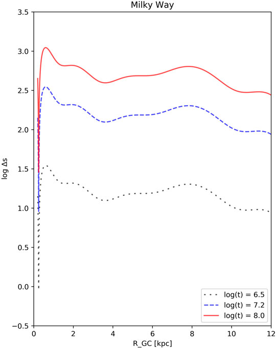
FIGURE 1. The orbital drift of the open cluster in our Galaxy from their host spiral arm as a function of the galacto-centric radius and time. The values of $\text{Δ}s$ under the logarithm are in parsec. Used parameters: Ω_p = 25 km/s/kpc, $\text{Δ}R=0.1$ kpc, rotation curve from Sofue et al. (1999), approximated by a high-degree polynomial ($\text{deg}>15$).

Braun (1991) studied the structure and kinematics of the Andromeda Galaxy (M 31). One of the results of this work is the spiral pattern velocity, Ω_p = 15 km/s/kpc. This helps us to explore the Andromeda Galaxy in the same way as our own Galaxy (assuming $\text{Δ}\mathrm{R}=0.1$ kpc). Figure 2 shows the resulting curves. It is immediately apparent that there is no global maximum (although we have cut out the region R < 0.5 kpc). The relative orbital drift varies only slightly with the galacto-centric radius, averaging at about 9, 90, and 285 pc, respectively. These are the smallest values among the four galaxies analyzed in this section. Indeed, the older clusters $\left[8.5>\text{log}\left(\text{age}\right)>8.0\right]$ appear to trace the spiral arms quite well (Caldwell et al., 2009). However, there is another point to be made about the older clusters, which we shall explore later on.

FIGURE 2

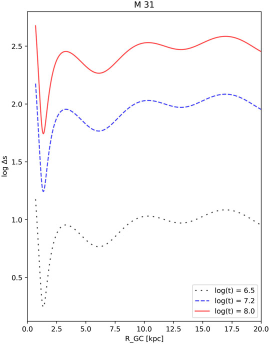
FIGURE 2. The orbital drift of the open cluster in M 31 from their host spiral arm as a function of the galacto-centric radius and time. The values of $\text{Δ}s$ under the logarithm are in parsec. Used parameters: Ω_p = 15 km/s/kpc, $\text{Δ}R=0.1$ kpc, rotation curve from Sofue et al. (1999), approximated by a high-degree polynomial ($\text{deg}>15$).

The next galaxy we want to inspect is M 51. It was discussed in Meidt et al. (2008) that there are quite obvious variations in the spiral pattern velocity of this galaxy at different galacto-centric radii. The pattern velocity starts from around 90 km/s/kpc in the inner regions of the galaxy and reduces down to about 50 km/s/kpc in the outer regions. For our analysis, we have used the latter value and $\text{Δ}\mathrm{R}=0.1$ kpc. Figure 3 shows that the situation is quite different from what we saw in the Milky Way. If we disregard the region R < 0.5 kpc, we see that there is no apparent global maximum and that $\text{Δ}\mathrm{s}$ oscillates around a well defined value of 34, 340, and 1,050 pc, respectively. The mean value of $\text{Δ}\mathrm{s}$ appears to be somewhat larger than in Milky Way. However, the situation would change considerably if we assumed that ${\text{Ω}}_p\ne \text{const}$. Let us try a function ${\text{Ω}}_p=\frac{108}{{\mathrm{R}}^{0.8}}$, which has a value 90.0 km/s/kpc at R = 1.2 kpc and 50.0 km/s/kpc at R = 2.5 kpc—the plot of $\mathrm{\Delta s}\left(\mathrm{R}\right)$ curves calculated based on this function is overlaid in Figure 3. The results for different functions ${\text{Ω}}_p$ clearly vary—the power law function seems to bring $\text{Δ}\mathrm{s}\left(\mathrm{R}\right)$ of M 51 closer to what we see in our Galaxy (where we, however, assumed constant ${\text{Ω}}_p$).

FIGURE 3

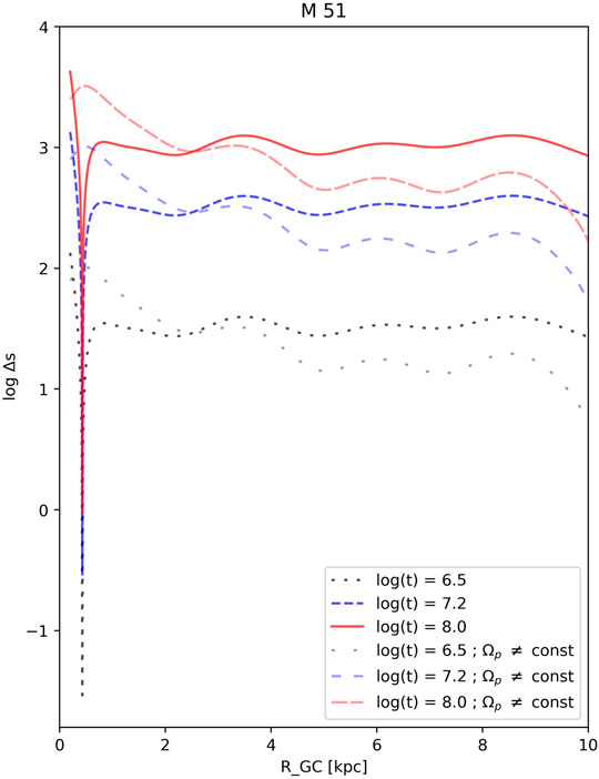
FIGURE 3. The orbital drift of the open cluster in M 51 from their host spiral arm as a function of the galacto-centric radius and time. The values of $\text{Δ}s$ under the logarithm are in parsec. Used parameters: ${\text{Ω}}_p=50-90$ km/s/kpc, $\text{Δ}R=0.1$ kpc, rotation curve from Sofue et al. (1999), approximated by a high-degree polynomial ($\text{deg}>15$).

Finally, Mulder and Combes (1996) showed that Ω_p = 14 km/s/kpc provides the best fit to the observations of NGC 3310. Once again, let us use the value $\text{Δ}\mathrm{R}=0.1$ kpc. The rotational curve of this galaxy was taken from Epinat et al. (2008). The function $\text{Δ}\mathrm{s}\left(\mathrm{R}\right)$ (Figure 4) is much more interesting than in the previous cases. Although the local maxima reach about the same values as we saw before, the typical values of the relative drift is generally smaller. Moreover, it is evident that there are multiple changes in the sign of $\text{Δ}\mathrm{s}$. It seems that NGC 3310 could be a bit more resistant to the breaking of the spiral distribution of clusters. However, there are no estimates of the width of the spiral arms of this galaxy and it is also worth mentioning that there is evidence of a recent merger (Miralles-Caballero et al., 2014), which could slightly complicate the situation.

FIGURE 4

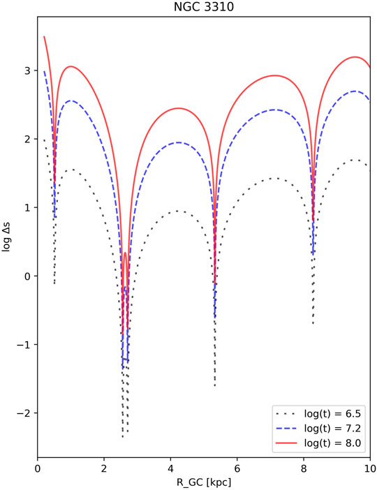
FIGURE 4. The orbital drift of the open cluster in NGC 3310 from their host spiral arm as a function of the galacto-centric radius and time. The values of $\text{Δ}s$ under the logarithm are in parsec. Used parameters: Ω_p =14 km/s/kpc, $\text{Δ}R=0.1$ kpc, rotation curve from Epinat et al. (2008), approximated by a high-degree polynomial ($\text{deg}>15$).

Another interesting approach is to set the rotation curve to be constant. In such case, the only remaining term in Eq. 2 is ${\text{Ω}}_p\text{Δ}\mathrm{R}$. For spiral arms rotating as rigid bodies, this will be a constant, therefore $\frac{\mathrm{d}\left(\mathrm{\Delta s}\right)}{\mathrm{dR}}=0$ and the relative drift $\text{Δ}\mathrm{s}\left(\mathrm{t}\right)\sim {10}^t$ will grow exponentially as a function of time.

3.4 Pattern Breaking—Velocity Dispersion

The velocity dispersion of an aggregate of bodies (we are interested solely in the bodies within individual galaxies) plays a significant role in the kinematic evolution of that aggregate. The magnitude of the dispersion varies from one system type to another. For stars in open clusters, one typically finds values of the order of ∼1 km/s (e.g., Kim et al., 2019, the value tends to increase with the age of the cluster). The velocity dispersion of young open clusters in their host galaxies reaches somewhat higher values (5–10 km/s in our Galaxy, Soubiran et al., 2018). More intermediate values are typically found in the stellar population of the disks of spiral galaxies—for our Galaxy, Gaia Collaboration et al. (2018c) found 10–50 km/s (different values for the radial, tangential, and vertical components). It is worth keeping in mind that the results are affected by the binary fraction, although the extent of this effect is currently unknown. Finally, an emphasis must be put of the fact that the velocity dispersion is a time-dependent quantity—it slowly increases over time (Yu and Liu, 2018).

If we set a cluster to follow the spiral arm perfectly (the term in the brackets of Eq. 1 is zero), the only remaining quantity is the velocity dispersion. In this example, we will be following the arm in its frame of reference and assume that the velocity dispersion is defined in the rotating frame. The random velocity vector is generated from a normal distribution, based on the dispersion, for each individual cluster—this vector is set to be constant. This is not physically acceptable and we shall return to this point in a moment. Right now, we would like to statistically examine, what is going to happen to the distribution of clusters if their orbital velocities randomly deviate from the pattern velocity.

For this, we can generate (for example) N = 20,000 values of $\text{Δ}\mathrm{s}$ for a given value of ${\sigma }_t$ and $\text{log}\left(\text{age}\right)$. Afterward, we can calculate the ratio $\mathrm{M/N}$, where M is the number of values for which the resulting drift $\text{Δ}\mathrm{s>}{\mathrm{s}}_{\lim }$. Parameter ${\mathrm{s}}_{\text{lim}}$ is set to be either 300 or 500 pc, which is comparable with the spiral arm widths in our Galaxy. Statistically, this should represent the probability that a cluster of given age is going to be able to drift beyond ${\mathrm{s}}_{\text{lim}}$, assuming that the kinematics is dominated by the given value of ${\sigma }_t$. The results for $6.5\le \text{log}\left(\text{age}\right)\le 8.0$ are presented in Figures 5, 6.

FIGURE 5

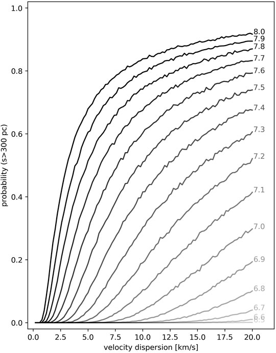
FIGURE 5. The estimated probability, that a randomly located cluster in a galaxy drifts from the spiral arm (its birthplace), as a function of the velocity dispersion. The simulation was done for multiple cluster ages. The cut-off value for $\text{Δ}s$ was chosen to be 300 pc. The pattern velocity is Ω_p = 25 km/s/kpc.

FIGURE 6

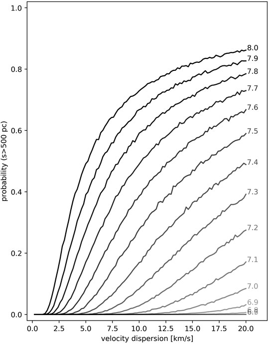
FIGURE 6. The estimated probability, that a randomly located cluster in a galaxy drifts from the spiral arm (its birthplace), as a function of the velocity dispersion. The simulation was done for multiple cluster ages. The cut-off value for $\text{Δ}s$ was chosen to be 500 pc. The pattern velocity is Ω_p = 25 km/s/kpc.

When assuming pure velocity dispersion (σ_t = 10.0 km/s) for the relative velocities of clusters compared to the motion of the spiral arm, the probability of a cluster drifting away from the arm becomes significant starting at ages between $\text{log}\left(\text{age}\right)=7.5$ and $\text{log}\left(\text{age}\right)=8.0$. We can see in Figures 5, 6 that the result depends strongly on the considered velocity dispersion value—this value is not very well constrained for the young clusters (Gieles et al., 2010).

The combination of the rotation curve velocity term (Milky Way) with the dispersion term is shown in Figure 7. While the velocity term of the rotation curve simply moves the clusters away from the spiral, the velocity dispersion destroys (over time) any information about the original distribution. This conclusion is comparable to what has been observed for M 51. It is clear in Figure 1 from Chandar et al. (2017) that clusters up to about $\text{log}\left(\text{age}\right)=8.0$ qualify as good tracers of the spiral arms. On the other hand, the observed older clusters in M 31 should not be good tracers of the spiral arms, assuming a velocity dispersion of σ_t > 10 km/s (Collins et al., 2011). This contradicts what has been indicated by observations—see Section 3.3. An observational bias is one possible explanation (not many clusters were used by Caldwell et al., 2009, Figure 10), but a more sophisticated model (Dobbs and Pringle, 2010) could also solve this problem.

FIGURE 7

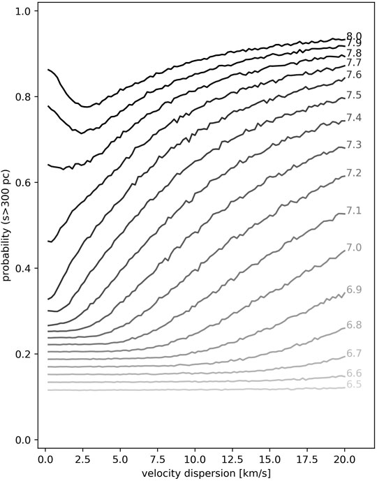
FIGURE 7. The estimated probability, that a randomly located cluster in a galaxy drifts from the spiral arm (its birthplace), as a function of the velocity dispersion. The simulation was done for multiple cluster ages. Orbital motion based on the rotation curve of the Milky Way is also included. The cut-off value for $\text{Δ}s$ was chosen to be 300 pc. The pattern velocity is Ω_p = 25 km/s/kpc. The decrease in the probability for higher ages is due to the fact, that rotation is enough to destroy the spiral structure—the velocity dispersion then slightly increases the chance that some of the clusters will stay near the arm (when compared with the zero-dispersion).

The pattern of the spiral arm in the distribution of open clusters does not break precisely in the way that was described here—this approach was used solely to estimate the effect of a random deviation of the orbital velocities from the pattern velocity. The velocity vector of clusters (or field stars) cannot be considered to be constant since the orbits are bound. Instead, a different approach must be taken. For example, the epicyclic approximation can be used to describe non-circular orbits. If we were to think about the velocity dispersion in the X and Y coordinates, the approach introduced here would not work—orbits need to be bound, which means that fictitious forces have to appear in the equations of motion.

Hydrodynamic simulations serve as a more precise tool for studying this problem (although they can become more time-consuming). For example, Dobbs and Pringle (2010) showed that different excitation models for the spiral arms result into different age-distributions of star clusters. In combination with observations, such approach can be used to determine the possible excitation mechanisms for different galaxies.

3.5 Simulating Local Spiral Arm

As a next step, we would like to compare a simulation of the breaking of the spiral pattern of the Local Arm with observations. For this, we shall use all of the kinematic parameters of our Galaxy mentioned in Section 3.1, together with the Gaia data. In what follows, we outline the overall procedure.

1. Simulate the Local Spiral Arm. For this we have used the model from Ringermacher and Mead (2009), using the parameters ${\text{par}}_{\mathrm{A}}=4.1$, ${\text{par}}_{\mathrm{B}}=0.3$ and ${\text{par}}_{\mathrm{N}}=3.7$. This gives us a fairly good representation of the Local Arm when compared with the model from Reid et al. (2014).

2. Create clusters at random positions along the arm. In our simulation, we have arbitrarily chosen 7,000 clusters to be produced. The width of the arm is simulated by randomizing position in the rectangular coordinates, reaching standard deviation of ∼300 pc at R∼8 kpc. This scatter can be scaled with the Galacto-centric radius but the change would be quite small in the spatial region we are interested in. Most of the open clusters studied in Gaia data are located within 4 kpc from the Sun, and one has to keep in mind that the distance error scales with the distance to the cluster.

3. For each cluster, simulate its members (a random number between 100 and 300 stars) using its location and a normal distribution with the width of 10 pc (corresponding to an upper value of typical cluster sizes, van den Bergh, 2006). This resembles the actual positions of cluster members in our simulation (although the kinematics will be used just for the clusters themselves, not for the individual member stars).

4. A good estimate of the absolute parallax error in Gaia DR2 is about 0.3 mas. The procedure converts the true distances into true parallaxes and applies the uncertainty values. For each star, the value of parallax is generated using a normal distribution centered at the true parallax, with the widths corresponding to the uncertainty. This simulates the process of measuring the parallaxes of the individual stars.

5. We shall assume that the parallaxes of cluster members form a normal distribution—the true parallax can be fairly precisely estimated by finding the center of the ϖ distribution of the cluster members. The procedure estimates the cluster distances d by inverting the central parallaxes. This approach is much more robust than simply inverting all of the parallaxes and finding the center of that distribution (however, not as good as using a Bayesian approach). For a more comprehensive insight into the conversion of parallaxes into distance, we redirect the reader to the interesting work by Luri et al. (2018).

6. Polar Galactic coordinates (from the perspective of the observer) are transformed again into rectangular coordinates, assuming that the Sun is located at (−8.3, 0.0) kpc. An arbitrary Gaussian probability distribution function (using the observed distance as a variable) is applied to simulate the fact that the more distant clusters can be missed. The cut-off between the revealed and the hidden clusters is set to be about 2 kpc away from the observer. We have to point out that only clusters along the spiral arm are simulated—we should still be able to recognize the spiral pattern in the distribution of clusters at this point.

7. A velocity vector is generated to each of the revealed clusters. It consists of the orbital velocity generated from the rotation curve of the Milky Way, and the x and y components of the velocity dispersion. Motion of each cluster can be described by the epicylic approximation. It is also worth mentioning that the uncertainty in the measurement of radial velocities should play a role similar to the one played by the velocity dispersion.

8. The clusters are allowed to move for a period of time A, after which the distribution of the clusters is checked again.

We shall assume that the kinematic effect of the tidal dissipation of clusters can be neglected, and clusters are allowed to follow orbits resulting from the epicylic approximation. Standard notation is implemented.

$\begin{array}{l}x\left(t\right)=x_0\text{sin}\left(\kappa t+\psi \right)\\ y\left(t\right)=y_0\text{cos}\left(\kappa t+\psi \right)\end{array}(3)$

where x is oriented in the radial direction and y is oriented in the tangential direction of the circular part of the motion, $x_0$ and $y_0$ are the amplitudes of the epicyclic motion, κ is the epicyclic frequency, and ψ is the initial phase of the epicyclic motion. We have used the velocities generated by the velocity dispersion as the initial values of $\dot{x}$ and $\dot{y}$. If we calculate the time-derivatives of Eq. 3, we can eliminated ψ from the equations

$\frac{{\dot{x}}^2}{x_0^2}+\frac{{\dot{y}}^2}{y_0^2}={\kappa }^2(4)$

and κ can be found from the relation $[\mathrm{R}\frac{{\text{dΩ}}^2}{\text{d}\mathrm{R}}+4{\text{Ω}}^2]$ evaluated at the radius of the circular part of the motion, ${\mathrm{R}}_0$. Moreover, $x_0$ and $y_0$ are linked by another relation

$\frac{x_0}{y_0}=\frac{\kappa \left(R_0\right)}{2\text{Ω}\left(R_0\right)}(5)$

We can combine Eqs. 4,Eqs. 5 to determine the unknown values of the amplitudes, and then return to the relations for $\dot{x}$ and $\dot{y}$ to find

$\text{tan}\left(\psi \right)=\frac{\dot{y}/y_0}{\dot{x}/x_0}(6)$

The motion in the polar Galacto-centric coordinate system is then described by the following two equations

$\begin{array}{l}\varphi \left(\mathrm{t}\right)={\varphi }_0+\text{Ω}t-\frac{y_0}{{\mathrm{R}}_0}\text{sin}\left(\kappa t+\psi \right)\\ \mathrm{R}\left(\mathrm{t}\right)={\mathrm{R}}_0+x_0\text{sin}\left(\kappa t+\psi \right)\end{array}(7)$

which can be easily transformed into the rectangular Galacto-centric coordinates. Finally, the spiral arm is also rotating in the Galaxy. To characterize the motion of the clusters with respect to the motion of the spiral arm, the positions of the individual clusters must be rotated by the angle $\alpha =-{\text{Ω}}_{p}t$. We emphasize that the pattern velocity ${\text{Ω}}_p$ is taken to be a constant.

We have simulated two situations—using only velocity dispersion, and assuming the full motion with the use of the epicyclic approximation. The resulting distributions are presented in Figures 8, 9 respectively. Pattern breaking, in the case of the epicyclic approximation, is dominated by the rotation curve. On the other hand, the velocity dispersion could not break the spiral pattern on its own—this is the result of the assumption of bound orbits (which is not considered in the pure-dispersion model). In reality, velocity dispersion vector increases with time, which would enhance the pattern breaking. Therefore, $\dot{\sigma }$ would be the driving mechanism for the spiral pattern breaking in terms of the dispersion.

FIGURE 8

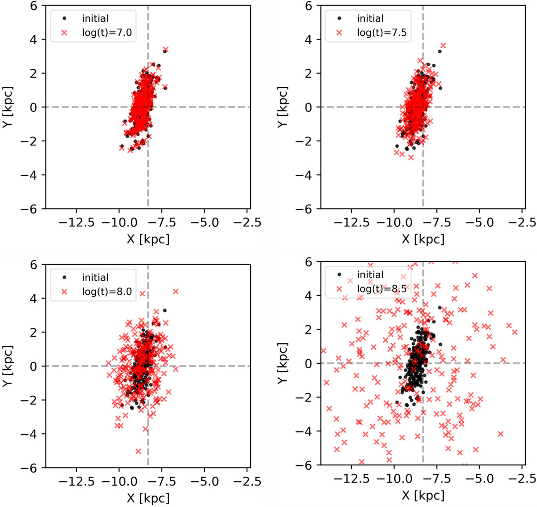
FIGURE 8. Breaking of the spiral pattern in the distribution of open clusters due to the dispersion of velocities introduced in the rotating frame of reference. As we discussed in the text, this situation is not physical. However, it still provides us with statistical information—even relatively small deviations from the orbital velocity (∼10 km/s) of the spiral arm would cause a breaking of the pattern.

FIGURE 9

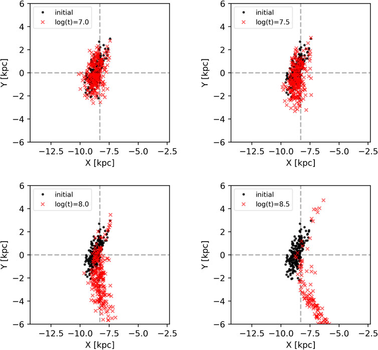
FIGURE 9. Breaking of the spiral pattern in the distribution of open clusters due to the difference between the orbital motion of the clusters and the pattern velocity of the rotating spiral arm. Velocity dispersion is introduced in the non-rotating frame of reference and describes the epicyclic motion. If the difference between the orbital velocity and the pattern velocity was zero, the cluster would not deviate (in this simple approximation) far from the spiral arm, it would rather oscillate around a point within the arm. The pattern breaking is dominated by the rotation curve—most of the clusters in the Local Arm are located beyond the corotation radius of this model, which results in the clusters trailing behind the spiral arm.

It is worth mentioning that the uncertainties in the observed distances played only a minor role in the simulation (unless clusters with distances $d>5.0$ kpc are taken into account). Much more dominant would be the uncertainties in the measurement of the velocity vector, if they were taken into account (we may assume that the uncertainties are hidden in the velocity dispersion term).

Clusters younger than $\text{log}\left(\text{age}\right)\sim 7.0$ follow the spiral arms very closely, as was expected. These objects represent a good tool for tracing spiral arms, even in the dynamically warmer galaxies. Unfortunately, most of such objects were missed in Cantat-Gaudin et al. (2018) who used primarily clusters with $\text{log}\left(\text{age}\right)>7.0$. Nevertheless, their distribution of the clusters younger than $\text{log}\left(\text{age}\right)\sim 8.0$ seems to represent the position of the spiral arms quite well, as was highlighted by the authors.

The main goal of this simulation was to study the situation after $\text{log}\left(\mathrm{t}\right)\sim 8.0$. Clearly, most of the clusters have drifted away from the spiral arm in both simulated cases. Although the simulation in Figure 8 is quite non-physical, it still provides a simple look at what happens with the distribution if only velocity dispersion is taken into account—the structure slowly dissipates into the surrounding area. The more realistic case is the assumption of nearly circular orbits (epicyclic approximation, Figure 9). Here we see that the distribution of the clusters changes from a spiral structure into a ring-like distribution, corresponding to a randomized position of the clusters within the Galactic disk.

3.6 Spiral Pattern in the Distribution of Open Clusters

We have seen that the distribution of open clusters changes based on their ages. However, when we observe clusters, the resulting data set almost always contains objects representing a mixture of ages. In principle, we can determine the cluster ages from the photometric data (isochrone fitting) but even if we ignored uncertainties, the resulting subsets of clusters would contain only a small number of objects. This is especially true for Cantat-Gaudin et al. (2018), where we see a lack of the younger clusters due to an observational bias. A small number of objects means that whatever statistical analysis we want to perform (for example, young clusters tracing a spiral arm), the results will turn out to be quite unreliable.

Fortunately, we can make use of everything we studied in the previous sections. We know that clusters younger than $\text{log}\left(\text{age}\right)\sim 8.0$ should follow the spiral arm they were born in quite tightly. On the other hand, older clusters should represent a background population. But how to display this situation? If we were to show all of the clusters, the map of their distribution would very messy. This results from the fact that a lower number of clusters are being born every 1 Myr than there are clusters older than them.

We find that breaking the distribution of clusters into three groups consisting of objects with ages around 3.1 (G6.5), 31 (G7.5) and 310 Myr (G8.5) works quite well. These groups are represented in Figure 10 by different symbols and colours. The assumed kinematics are the same as in the previous section (epicyclic approximation, Ω_p = 25 km/s/kpc, rotation curve of the Milky Way, the same spiral arm as described above), but there are two spiral arms (the second one is created by rotating the original one by 180° around the Galactic center). The simulation starts at t = 0 Myr and continues with a time-step $\text{Δ}t=2$ Myr. At the beginning of each step, 100 clusters are born randomly across the whole arm, and the simulation stops at t = 1000 Myr. At this point, the distribution should be stable, and the positions of the clusters are plotted into Figure 10.

FIGURE 10

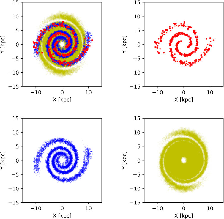
FIGURE 10. Maps of the cluster distribution estimated for a kinematic model of our Galaxy. The clusters were separated into three groups: G6.5, G7.5, and G8.5. (A): the composite picture of the distribution; red crosses and blue triangles follow the spiral arm quite closely. (B): clusters with ages around 3.1 Myr. (C): clusters with ages around 31 Myr. (D): clusters with ages around 310 Myr.

In the subplots, the data points are scaled using a Gaussian distribution centered at the age of the given group, with a width of 20% of this value. This means that if we were to follow one of the clusters in time, it would:

• First, appear at an age of about 6.5 as a red cross, then it would very quickly fade away

• It becomes visible again as a blue triangle at an age of about 7.3, afterwards fades at about 7.6

• Lastly, the cluster appears as a yellow circle at 8.4 for a significantly longer amount of time and disappears at an age of 8.6

The third group consists mostly of clusters just below the upper bound of the life-span of a typical open cluster in our Galaxy (∼1 Gyr, Spitzer, 1958).

The distribution of clusters in Figure 10 looks just as expected. The younger clusters from the groups G6.5 and G7.5 closely follow the spiral arms, with only a small angular lag between them (depends of the Galacto-centric radius, the lag is close to zero near the corotation). The group G8.5 shows that the distribution of clusters in the inner region of our Galaxy randomizes while the outer region should retain its spiral structure under our kinematic assumptions. However, this older distribution lags significantly behind the actual position of the spiral arm.

4 Diffuse Interstellar Bands as Tracers of Spiral Arms

Diffuse interstellar bands (DIBs) is a designation of a several 100 mysterious absorption features, most likely originating from the interstellar medium. They appear in the lines of sight toward stars of different spectral types, although they are most prominent in the spectra of reddened hot stars. Most of the DIBs are quite narrow (FWHM < 0 nm), with only several exceptions (e.g., the strong bands at 443.0, 578.0, and 628.4 nm). These bands have been observed not only within Milky Way but also in other galaxies:

• Magellanic Clouds (Ehrenfreund et al., 2002)

• M 31 (Cordiner et al., 2008a)

• M 33 (Cordiner et al., 2008b)

• NGC 1448 (Sollerman et al., 2005)

• NGC 4038/NGC 4039 (Monreal-Ibero et al., 2018)

• NGC 1614, NGC 1808, NGC 2146, NGC 3256, NGC 6240, M 82, and IRAS 10565 + 2448 (Heckman and Lehnert, 2000)

Although many DIBs are located near regions contaminated by other lines/bands (for example, the overlap of the telluric band with the DIB at 628.4 nm), some remain easily resolved in the most of the spectra (e.g., 661.4 nm band). Given their characteristically narrow profiles, these bands could be quite useful for studying the interstellar medium of galaxies, depending on the spectral region, resolution and on the choice of the DIBs.

One of the common properties of the individual DIBs is that they are somehow correlated with the interstellar reddening (Merrill and Wilson, 1938). Although this correlation is often described as linear, the relation between the reddening [typically $E\left(B-V\right)$] and the strength of the DIBs (usually described by their equivalent widths, EWs) is far more complicated. For start, the distribution of the points in the reddening-EW diagrams is usually quite broad. Moreover, if we just use only one DIB, we will find that the correlation differs between different lines of sight in our Galaxy (see, for example, Piecka and Paunzen, 2020).

Some of the DIBs can be shown to posses quite complicated profiles using high-resolution spectroscopy (ideally R>100,000). We mention two examples, the bands at 579.7 and 661.4 nm, the profiles of which differ in many ways. Curiously, the origin of these structures is not yet well understood. According to Cami et al. (2004), the most likely explanation is that 1) the structure is the result of unresolved ro-vibrational structure of the molecules, or 2) the isotope effect dominates in the structure. The latter option is typically dismissed due to the observed variations in the relative positions of the individual peaks in the bands profile.

4.1 Origin of the Diffuse Interstellar Bands

Discovered about 100 years ago (Heger, 1922), vast majority of the DIBs remain unidentified to this date. Only quite recently, several bands were attributed to the molecular ion ${\mathrm{C}}_{60}^{+}$ by Campbell et al. (2015). This assignment was later supported by the observations (Cordiner et al., 2019). There are many other molecules which were considered as carriers of some of the DIBs, for example: different polycyclic aromatic hydrocarbons (PAHs, e.g., see Salama et al., 2011), carbon chains (Maier et al., 2004), propadienylidene l-C₃H₂ (Maier et al., 2011). However, these DIBs were found to be located outside the regions of bands of the corresponding molecules. The verification is based on the high-precision laboratory spectroscopy.

As was mentioned above, correlation between DIBs and the reddening varies across the sky (and most likely even in the radial direction). Not all of the DIBs are always present in a given line of sight and the EW-ratios of a pair of DIBs are usually inconsistent, except for the well correlated pair at 619.6 and 661.4 nm (Krełowski et al., 2016). Together with the variations in the profiles of DIBs, this would suggest that the number of carriers depends heavily on the conditions within the probed medium. Moreover, there have to be multiple different species in order to explain the observed EW-ratios. Jenniskens et al. (1994) showed that one of the most important properties of the medium surrounding the DIB carriers is the intensity of the UV radiation field. Generally, carriers seem to be more abundant in the regions with high intensity UV fields (such as the Orion Nebula, M 42, mentioned in the cited paper) than in the dense molecular regions. However, this is not a strict rule—Jenniskens et al. (1994) pointed out that the 628.4 nm DIB behaves differently than described.

One topic which remains seriously unexplored is the formation of the carriers of DIBs. Presently, there are no specific theories about the processes leading to the creation of the DIB-carriers in the interstellar medium (ISM). Very important questions are still left unanswered:

• Are these species formed in situ, or do they exist for an extended amount of time (albeit in several different states)?

• Do these species form during the destruction/formation processes of interstellar dust grains, or is their creation unrelated to dust?

• Can these species be born in stellar outflows?

We can learn much from the observed spectra. For example, studies of the planetary nebulae have shown that fullerenes (such as C₆₀) can be found in circum-stellar medium or in stellar outflows (García-Hernández and Díaz-Luis, 2013). Such relatively simple and very stable molecules are thought to be the product of larger molecules being broken down (Berné et al., 2015). The reason why C₆₀ appears as the most abundant of the fullerenes is its stability. If we accepted this model (top-down formation) to be the most realistic, we could study the details of the formation processes. However, this is only usable for this single molecule as (at least) dozens of other carriers remain unidentified. Can the story behind the other molecules be the same as for the fullerenes?

The interstellar environment puts strict physical constraints on the structure of the carriers—they are most likely moderately sized organic or carbonaceous molecules, $\mathrm{N}\left(\text{C}\right)>20$, with highly symmetric structures providing resistance to the UV photo-dissociation. Recently, Omont et al. (2019) brought into attention a subclass of PAHs, the polyacenes, which easily fulfill all of the required properties. Unfortunately, high-quality laboratory spectra are only available for a small number of these molecular species.

4.2 Mapping the Interstellar Medium

It might seem that these bands could, in principle, be quite good tracers of the spiral arms. This is due to the much larger star-formation rates in the arms than in the space between them. Such regions can become rich in the nebulae such as M 42, which should produce larger absorption in the DIBs. However, we should keep in mind the following: although a given DIB is a good tracer of a specific set of conditions, the specifics of these conditions are poorly understood.

An interesting map of the infrared DIB at 1.5273 μm was presented by Zasowski et al. (2015). Their work is based on the spectra of ∼60,000 stars from SDSS/APOGEE. Unfortunately, no spiral arm is visible in their map.

Elyajouri and Lallement (2019) presented over 100,000 measurements of the 1.5273 μm DIB (also SDSS/APOGEE). The lines of sight cover much of the region between $l=0^{\circ }$ and $l={270}^{\circ }$. We wanted to use these results to construct maps similar to those from Zasowski et al. (2015). When mapping diffuse interstellar bands, it can be rewarding to also look at $\text{EW}/{\mathrm{A}}_{\mathrm{V}}$, the ratio of the EW and the extinction value in that direction (authors adopted values from Starhorse database). In Figure 11, we show the maps based on the results from Elyajouri and Lallement (2019). The ratios are shown in the upper plot, the EWs in the lower plot. Distances were calculated by inverting parallaxes ϖ from Gaia DR2, restricting ourselves to |z| < 100 pc. We would like to point out that the parallax inversion may lead to distortions in Figure 11 at distances (from the center) larger than about ∼1 kpc. To improve the situation, we excluded all lines of sight for which the stellar parallaxes from Gaia DR2 have relative errors $e_{\varpi }/\varpi >0.20$. The maps were created by binning targets in cells (200 × 200 pc) and using the median of the mapped quantity in for each cell. Finally, the intensity of the cells reflects the magnitude of the quantity—larger value means darker cell. For the ratios, we have introduced a cut-off value $\text{EW}/{\mathrm{A}}_{\mathrm{V}}=1$, meaning that all cells with larger values than this limit are equal in the map (darkest black). The intensity then drops and is equal to the ratio value. For the EWs map, the intensities are scaled by the maximum value of median (EW), which in our case is 491.92 mÅ.

FIGURE 11

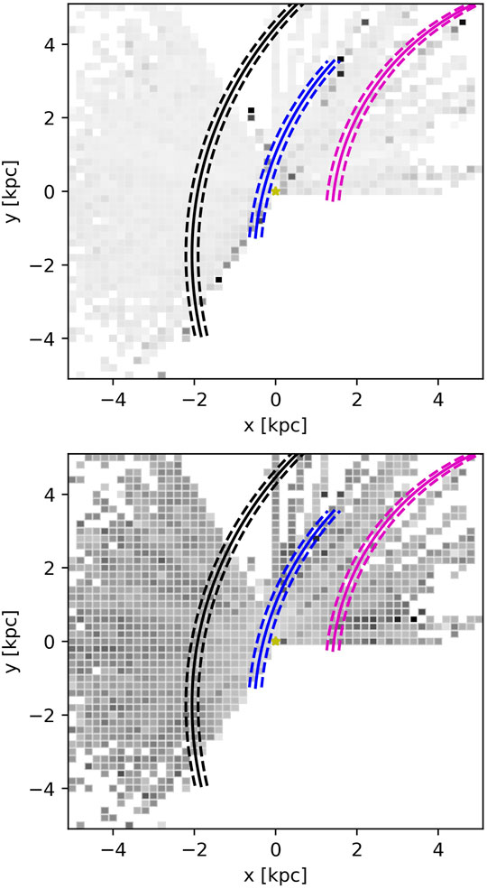
FIGURE 11. The maps of the DIB at 1.5273 μm, based on the data from Elyajouri and Lallement (2019). The upper plot displays the distribution of the ratios $\text{EW}/A_V$, the lower plot shows the distribution of EWs. The darker the cell, the higher the value. The coordinates are centered at the position of the Sun (not the Galacto-centric coordinates). The nearby spiral arms from Reid et al. (2014) are displayed with different colours (black—Perseus Arm, blue—Local Arm, magenta—Sagittarius Arm); the corresponding dotted lines emphasize their widths.

The results are comparable to what Zasowski et al. (2015) showed. In the near vicinity of the Sun, the use of the DIBs for tracing Galactic arms is fairly limited. The biggest problem with the maps of EWs is that their values are always integrated in the line of sight. There is a possible solution to this problem. If we have two targets which are very close to each other on the sky but distant in the parallax, we could subtract the EW of the closer target from the more distant one, leaving potential only the amount of absorption from the region beyond the closer target. However, there are several difficulties. Firstly, the observed quantities (EWs, parallaxes) are accompanied by uncertainties, which may affect the result. Secondly, we have no prior knowledge about the variation of the EWs across the sky in the observed area around the target stars—these variations may have a large impact on the suggested subtraction procedure. Finally, if we look at the distance-EW diagrams, we shall see a significant scatter. The EWs do not seem to follow any curve in such plots, instead they are somehow distributed from zero up to an upper limit value, which depends on the distance. We can either attempt to extract these upper limits per distance, or median values, but neither of those provides a precise measure which is required for our procedure.

The ratios $\text{EW}/{\mathrm{A}}_{\mathrm{V}}$ can be somewhat more useful when looking at the spatial maps of DIBs. The idea is to use the mentioned infrared DIB, because of its tight correlation with the extinction (Zasowski et al., 2015). Indeed, the darkest cells in the upper plot of Figure 11 seem to follow the Local Arm. However, this may be a result of some unknown bias. However, this approach can be a bit problematic. This is due to the introduction of the division of by $A_V$ (which is also accompanied by an uncertainty).

In Figure 2, Monreal-Ibero et al. (2018) presented maps of the 578.0 and 579.7 nm DIBs in the Antennae Galaxies (NGC 4038/NGC 4039). Their maps cover a large part of the northern spiral arm. Moreover, the carriers of the studied DIBs seem to be fairly abundant in some regions of the arm. Regardless, a closer inspection of the map of 578.0 nm DIB shows that the EW varies across the arm—the arm passes through regions with both, relatively strong and weak absorption in the DIBs. The situation is the same outside of the arm. In this case, the chosen band appears as a poor choice of a tracer of the spiral structure of these galaxies. The DIB at 579.7 nm covers somewhat smaller regions than the one at 578.0 nm. Its map shows that the strongest absorption is located within the region where the strongest optical absorption is observed. Again, no spiral structure can be distinguished in the map.

To our knowledge, no other detailed maps of other galaxies have been published. Theoretically, the ability of DIBs to probe interstellar medium with a narrow range of possible properties can be very handy. The practicality of using these tools is limited by the spectroscopic resolution, the signal to noise ratio (which becomes a very important factor when studying distant galaxies), and finally the ability to derive the parameters of the band-profiles. It remains to be seen whether DIBs will become useful as tracers of the galactic structure.

5 Conclusion

We have based our simulations of motion of open clusters on some of the newest data from Gaia (velocity dispersion) and on the rotation curve of the Milky Way. We have constructed a simple mathematical apparatus for the analysis of the distribution of open clusters when compared with the spiral arm they originate from. As expected, the older clusters seem to move away from the arm—this makes such clusters poor tracers of the spiral structure of galaxies.

Although the investigation of spiral arms was not the main contribution of the work Cantat-Gaudin et al. (2018), they have used older clusters for demonstrating the possibility of using Gaia for this purposes. We should remind ourselves that such results must be viewed upon with care—only the young open clusters (younger than about 100 Myr, but even younger should be preferred) can be used to get reliable results. It is worth mentioning that the number of clusters younger than about 30 Myr is very low in the cited work. Despite this, the nearby open clusters are found near the relevant spiral arms near the Sun.

Figure 8 and Figure 9 display how the distribution of open clusters breaks away from the spiral structure after some amount of time. The former shows how this would happen, if the clusters had moved away from the arm with random velocities—although an non-physical solution, this demonstrates how the difference between the motion of physical objects of the host galaxy and the motion of the spiral arm must result in pattern breaking. The second plot is based on the epicylic approximation of the cluster orbits. After some time (>300 Myr), the distribution turns from being a spiral into a ring-like structure.

In Section 3.6, we have demonstrated purely kinematic simulation of open clusters being born in the spiral arms. Dynamical processes could further enhance the effect of pattern breaking in the distribution of open clusters. The model of the simulated galaxy is close to our present view of the Milky Way. We can see that, at some point, the distribution of the older clusters winds up.

Although greatly inferior to the N-body and hydrodynamic simulations, we have shown that the described approach proves to be useful for taking an initial look at the observed data. It makes it possible to analyze multiple different galaxies in a short time. However, more sophisticated methods should be preferred when attempting to study the problem at hand in greater detail.

Finally, we have studied the map of the DIB at 1.5273 μm (Figure 11). There does not seem to be any clear spiral structure present in the map, although something appear in the vicinity of the Local Arm—it is difficult to distinguish whether this is a result of a bias (possibly caused by the inversion of parallaxes). The lack of a larger number of measurements in the other DIBs prevents us from analyzing the map at different wavelengths. Based on this result and comparing with maps of other galaxies in the literature, we conclude that DIBs appear to be ineffective when tracing spiral arms. However, we do not rule out the possibility that a different approach or additional data could change this status.

Data Availability Statement

The raw data supporting the conclusions of this article will be made available by the authors, without undue reservation.

Author Contributions

MP: compilation of the literature and available data, programming and implementation of the simulation, interpretation of the results, generating of the figures, analysis of the DIBs, writing the article. EP: compilation of the literature and available data, interpretation of the results, writing the article.

Funding

This work was supported by MUNI/A/1482/2019 and MUNI/A/1206/2020, Masaryk University, Faculty of science.

Conflict of Interest

The authors declare that the research was conducted in the absence of any commercial or financial relationships that could be construed as a potential conflict of interest.

Acknowledgments

This research has made use of the WEBDA database, operated at the Department of Theoretical Physics and Astrophysics of the Masaryk University, the SIMBAD database, operated at CDS, Strasbourg, France and NASA’s Astrophysics Data System. This work presents results from the European Space Agency (ESA) space mission Gaia. Gaia data are being processed by the Gaia Data Processing and Analysis Consortium (DPAC). Funding for the DPAC is provided by national institutions, in particular the institutions participating in the Gaia MultiLateral Agreement (MLA). The Gaia mission website is https://www.cosmos.esa.int/gaia. The Gaia archive website is https://archives.esac.esa.int/gaia. The rotation curves were based on a polynomial fit to the data from http://www.ioa.s.u-tokyo.ac.jp/∼sofue/RC99/rc99.htm.

References

Arenou, F., Luri, X., Babusiaux, C., Fabricius, C., Helmi, A., Muraveva, T., et al. (2018). Gaia Data Release 2. A&A 616, A17. doi:10.1051/0004-6361/201833234

CrossRef Full Text | Google Scholar

Arenou, F., Luri, X., Babusiaux, C., Fabricius, C., Helmi, A., Robin, A. C., et al. (2017). Gaia Data Release 1. A&A 599, A50. doi:10.1051/0004-6361/201629895

CrossRef Full Text | Google Scholar

Balaguer-Núñez, L., López del Fresno, M., Solano, E., Galadí-Enríquez, D., Jordi, C., Jimenez-Esteban, F., et al. (2020). Clusterix 2.0: a Virtual Observatory Tool to Estimate Cluster Membership Probability. MNRAS 492, 5811–5843. doi:10.1093/mnras/stz3610

CrossRef Full Text | Google Scholar

Baratella, M., D’Orazi, V., Carraro, G., Desidera, S., Randich, S., Magrini, L., et al. (2020). The Gaia-ESO Survey: a New Approach to Chemically Characterising Young Open Clusters. A&A 634, A34. doi:10.1051/0004-6361/201937055

CrossRef Full Text | Google Scholar

Bastian, U., and Röser, S. (1993). PPM Star Catalogue. Positions and Proper Motions of 197179 Stars South of -2.5 Degrees Declination for Equinox and Epoch J2000. Heidelberg, Germany: Spektrum Akademischer Verlag.

Baumgardt, H., and Kroupa, P. (2007). A Comprehensive Set of Simulations Studying the Influence of Gas Expulsion on star Cluster Evolution. MNRAS 380, 1589–1598. doi:10.1111/j.1365-2966.2007.12209.x

CrossRef Full Text | Google Scholar

Bekki, K., Koribalski, B. S., Ryder, S. D., and Couch, W. J. (2005). Massive H I Clouds with No Optical Counterparts as High-Density Regions of Intragroup H I Rings and Arcs. Monthly Notices R. Astronomical Soc. Lett. 357, L21–L25. doi:10.1111/j.1745-3933.2005.08625.x

CrossRef Full Text | Google Scholar

Berné, O., Montillaud, J., and Joblin, C. (2015). Top-down Formation of Fullerenes in the Interstellar Medium. A&A 577, A133. doi:10.1051/0004-6361/201425338

CrossRef Full Text | Google Scholar

Beuther, H., Walsh, A., Schilke, P., Sridharan, T. K., Menten, K. M., and Wyrowski, F. (2002). CH3OH and H2O Masers in High-Mass star-forming Regions. A&A 390, 289–298. doi:10.1051/0004-6361:20020710

CrossRef Full Text | Google Scholar

Binney, J., and Tremaine, S. (2008). James Binney and Scott Tremaine. ISBN 978-0-691-13026-2 (HB). Galactic Dynamics. Second Edition, Princeton, NJ: Princeton University Press. doi:10.1515/9781400828722

CrossRef Full Text

Bobylev, V. V., Bajkova, A. T., Rastorguev, A. S., and Zabolotskikh, M. V. (2021). Analysis of Galaxy Kinematics Based on Cepheids from the Gaia DR2 Catalogue. MNRAS 502, 4377–4391. doi:10.1093/mnras/stab074

CrossRef Full Text | Google Scholar

Borissova, J., Kurtev, R., Amarinho, N., Alonso-García, J., Ramírez Alegría, S., Bernal, S., et al. (2020). Small-scale star Formation as Revealed by VVVX Galactic Cluster Candidates. MNRAS 499, 3522–3533. doi:10.1093/mnras/staa3045

CrossRef Full Text | Google Scholar

Bossini, D., Vallenari, A., Bragaglia, A., Cantat-Gaudin, T., Sordo, R., Balaguer-Núñez, L., et al. (2019). Age Determination for 269 Gaia DR2 Open Clusters. A&A 623, A108. doi:10.1051/0004-6361/201834693

CrossRef Full Text | Google Scholar

Bouwman, J., Castellanos, P., Bulak, M., Terwisscha van Scheltinga, J., Cami, J., Linnartz, H., et al. (2019). Effect of Molecular Structure on the Infrared Signatures of Astronomically Relevant PAHs. A&A 621, A80. doi:10.1051/0004-6361/201834130

CrossRef Full Text | Google Scholar

Bragaglia, A., and Tosi, M. (2006). The Bologna Open Cluster Chemical Evolution Project: Midterm Results from the Photometric Sample. Astron. J. 131, 1544–1558. doi:10.1086/499537

CrossRef Full Text | Google Scholar

Braun, R. (1991). The Distribution and Kinematics of Neutral Gas in M31. ApJ 372, 54. doi:10.1086/169954

CrossRef Full Text | Google Scholar

Caldwell, N., Harding, P., Morrison, H., Rose, J. A., Schiavon, R., and Kriessler, J. (2009). Star Clusters in M31. I. A Catalog and a Study of the Young Clusters. Astronomical J. 137, 94–110. doi:10.1088/0004-6256/137/1/94

CrossRef Full Text | Google Scholar

Cami, J., Salama, F., Jiménez-Vicente, J., Galazutdinov, G. A., and Krełowski, J. (2004). The Rotational Excitation Temperature of the λ6614 Diffuse Interstellar Band Carrier. ApJ 611, L113–L116. doi:10.1086/423991

CrossRef Full Text | Google Scholar

Campbell, E. K., Holz, M., Gerlich, D., and Maier, J. P. (2015). Laboratory Confirmation of C60+ as the Carrier of Two Diffuse Interstellar Bands. Nature 523, 322–323. doi:10.1038/nature14566

PubMed Abstract | CrossRef Full Text | Google Scholar

Cantat-Gaudin, T., Anders, F., Castro-Ginard, A., Jordi, C., Romero-Gómez, M., Soubiran, C., et al. (2020). Painting a Portrait of the Galactic Disc with its Stellar Clusters. A&A 640, A1. doi:10.1051/0004-6361/202038192

CrossRef Full Text | Google Scholar

Cantat-Gaudin, T., Jordi, C., Vallenari, A., Bragaglia, A., Balaguer-Núñez, L., Soubiran, C., et al. (2018). A Gaia DR2 View of the Open Cluster Population in the Milky Way. A&A 618, A93. doi:10.1051/0004-6361/201833476

CrossRef Full Text | Google Scholar

Castro-Ginard, A., Jordi, C., Luri, X., Álvarez Cid-Fuentes, J., Casamiquela, L., Anders, F., et al. (2020). Hunting for Open Clusters in Gaia DR2: 582 New Open Clusters in the Galactic Disc. A&A 635, A45. doi:10.1051/0004-6361/201937386

CrossRef Full Text | Google Scholar

Castro-Ginard, A., Jordi, C., Luri, X., Cantat-Gaudin, T., and Balaguer-Núñez, L. (2019). Hunting for Open Clusters in Gaia DR2: the Galactic Anticentre. A&A 627, A35. doi:10.1051/0004-6361/201935531

CrossRef Full Text | Google Scholar

Castro-Ginard, A., Jordi, C., Luri, X., Julbe, F., Morvan, M., Balaguer-Núñez, L., et al. (2018). A New Method for Unveiling Open Clusters in Gaia. A&A 618, A59. doi:10.1051/0004-6361/201833390

CrossRef Full Text | Google Scholar

Chandar, R., Chien, L.-H., Meidt, S., Querejeta, M., Dobbs, C., Schinnerer, E., et al. (2017). Clues to the Formation of Spiral Structure in M51 from the Ages and Locations of Star Clusters. ApJ 845, 78. doi:10.3847/1538-4357/aa7b38

CrossRef Full Text | Google Scholar

Chrobáková, Ž., López-Corredoira, M., Sylos Labini, F., Wang, H.-F., and Nagy, R. (2020). Gaia-DR2 Extended Kinematical Maps. A&A 642, A95. doi:10.1051/0004-6361/202038736

CrossRef Full Text | Google Scholar

Collins, M. L. M., Chapman, S. C., Ibata, R. A., Irwin, M. J., Rich, R. M., Ferguson, A. M. N., et al. (2011). The Kinematic Identification of a Thick Stellar Disc in M31★†. MNRAS 413, 1548–1568. doi:10.1111/j.1365-2966.2011.18238.x

CrossRef Full Text | Google Scholar

Conti, P. S., and Crowther, P. A. (2004). MSX Mid-infrared Imaging of Massive star Birth Environments - II. Giant H Ii Regions. MNRAS 355, 899–917. doi:10.1111/j.1365-2966.2004.08367.x

CrossRef Full Text | Google Scholar

Cordiner, M. A., Cox, N. L. J., Trundle, C., Evans, C. J., Hunter, I., Przybilla, N., et al. (2008a). Detection of Diffuse Interstellar Bands in M 31. A&A 480, L13–L1. doi:10.1051/0004-6361:20079309

CrossRef Full Text | Google Scholar

Cordiner, M. A., Linnartz, H., Cox, N. L. J., Cami, J., Najarro, F., Proffitt, C. R., et al. (2019). Confirming Interstellar C60 + Using the Hubble Space Telescope. ApJ 875, L28. doi:10.3847/2041-8213/ab14e5

CrossRef Full Text | Google Scholar

Cordiner, M. A., Smith, K. T., Cox, N. L. J., Evans, C. J., Hunter, I., Przybilla, N., et al. (2008b). Diffuse Interstellar Bands in M 33. A&A 492, L5–L8. doi:10.1051/0004-6361:200810906

CrossRef Full Text | Google Scholar

Dias, W. S., Alessi, B. S., Moitinho, A., and Lépine, J. R. D. (2002). New Catalogue of Optically Visible Open Clusters and Candidates. A&A 389, 871–873. doi:10.1051/0004-6361:20020668

CrossRef Full Text | Google Scholar

Dias, W. S., and Lépine, J. R. D. (2005). Direct Determination of the Spiral Pattern Rotation Speed of the Galaxy. ApJ 629, 825–831. doi:10.1086/431456

CrossRef Full Text | Google Scholar

Dias, W. S., Monteiro, H., Lépine, J. R. D., and Barros, D. A. (2019). The Spiral Pattern Rotation Speed of the Galaxy and the Corotation Radius with Gaia DR2. MNRAS 486, 5726–5736. doi:10.1093/mnras/stz1196

CrossRef Full Text | Google Scholar

Dias, W. S., Monteiro, H., Moitinho, A., Lépine, J. R. D., Carraro, G., Paunzen, E., et al. (2021). Updated Parameters of 1743 Open Clusters Based on Gaia DR2. MNRAS 504, 356–371. doi:10.1093/mnras/stab770

CrossRef Full Text | Google Scholar

Díaz-García, S., Salo, H., Knapen, J. H., and Herrera-Endoqui, M. (2019). The Shapes of Spiral Arms in the S4G Survey and Their Connection with Stellar Bars. A&A 631, A94. doi:10.1051/0004-6361/201936000

CrossRef Full Text | Google Scholar

Dobbs, C. L., and Pringle, J. E. (2010). Age Distributions of star Clusters in Spiral and Barred Galaxies as a Test for Theories of Spiral Structure. MNRAS 409, 396–404. doi:10.1111/j.1365-2966.2010.17323.x

CrossRef Full Text | Google Scholar

Ehrenfreund, P., Cami, J., Jiménez-Vicente, J., Foing, B. H., Kaper, L., van der Meer, A., et al. (2002). Detection of Diffuse Interstellar Bands in the Magellanic Clouds. ApJ 576, L117–L120. doi:10.1086/343731

CrossRef Full Text | Google Scholar

Elmegreen, B. G., and Hunter, D. A. (2010). On the Disruption of Star Clusters in a Hierarchical Interstellar Medium. ApJ 712, 604–623. doi:10.1088/0004-637X/712/1/604

CrossRef Full Text | Google Scholar

Elyajouri, M., and Lallement, R. (2019). Updated Extraction of the APOGEE 1.5273 μm Diffuse Interstellar Band: a Planck View on the Carrier Depletion in Dense Cores. A&A 628, A67. doi:10.1051/0004-6361/201834452

CrossRef Full Text | Google Scholar

Epinat, B., Amram, P., Marcelin, M., Balkowski, C., Daigle, O., Hernandez, O., et al. (2008). GHASP: an Hα Kinematic Survey of Spiral and Irregular Galaxies - VI. New Hα Data Cubes for 108 Galaxies. MNRAS 388, 500–550. doi:10.1111/j.1365-2966.2008.13422.x

CrossRef Full Text | Google Scholar

Er, X.-Y., Jiang, Z.-B., and Fu, Y.-N. (2009). A Numerical Simulation Study of Mass Segregation in Embedded Stellar Clusters. Chin. Astron. Astrophys. 33, 139–150. doi:10.1016/j.chinastron.2009.03.012

CrossRef Full Text | Google Scholar

Faherty, J. K., Bochanski, J. J., Gagné, J., Nelson, O., Coker, K., Smithka, I., et al. (2018). New and Known Moving Groups and Clusters Identified in a Gaia Comoving Catalog. ApJ 863, 91. doi:10.3847/1538-4357/aac76e

CrossRef Full Text | Google Scholar

Fernández, D., Figueras, F., and Torra, J. (2001). Kinematics of Young Stars. A&A 372, 833–850. doi:10.1051/0004-6361:20010366

CrossRef Full Text | Google Scholar

Fitzpatrick, E. L. (1999). Correcting for the Effects of Interstellar Extinction. Publ. Astron. Soc. Pac. 111, 63–75. doi:10.1086/316293

CrossRef Full Text | Google Scholar

Gaburov, E., Gualandris, A., and Portegies Zwart, S. (2008). On the Onset of Runaway Stellar Collisions in Dense star Clusters - I. Dynamics of the First Collision. Monthly Notices RAS 384, 376–385. doi:10.1111/j.1365-2966.2007.12731.x

CrossRef Full Text | Google Scholar

Gaia Collaboration, Babusiaux, C., van Leeuwen, F., Barstow, M. A., Jordi, C., Vallenari, A., et al. (2018a). Gaia Data Release 2. Observational Hertzsprung-Russell Diagrams. A&A 616, A10. doi:10.1051/0004-6361/201832843

CrossRef Full Text | Google Scholar

Gaia Collaboration, Brown, A. G. A., Vallenari, A., Prusti, T., de Bruijne, J. H. J., Babusiaux, C., et al. (2018b). Gaia Data Release 2. Summary of the Contents and Survey Properties. A&A 616, A1. doi:10.1051/0004-6361/201833051

CrossRef Full Text | Google Scholar

Gaia Collaboration, Katz, D., Antoja, T., Romero-Gómez, M., Drimmel, R., Reylé, C., et al. (2018c). Gaia Data Release 2. Mapping the Milky Way Disc Kinematics. A&A 616, A11. doi:10.1051/0004-6361/201832865

CrossRef Full Text | Google Scholar

Gaia Collaboration, van Leeuwen, F., Vallenari, A., Jordi, C., Lindegren, L., Bastian, U., et al. (2017). Gaia Data Release 1. Open Cluster Astrometry: Performance, Limitations, and Future Prospects. A&A 601, A19. doi:10.1051/0004-6361/201730552

CrossRef Full Text | Google Scholar

García-Hernández, D. A., and Díaz-Luis, J. J. (2013). Diffuse Interstellar Bands in Fullerene Planetary Nebulae: the Fullerenes - Diffuse Interstellar Bands Connection. A&A 550, L6. doi:10.1051/0004-6361/201220919

CrossRef Full Text | Google Scholar

Geen, S., Soler, J. D., and Hennebelle, P. (2017). Interpreting the star Formation Efficiency of Nearby Molecular Clouds with Ionizing Radiation. MNRAS 471, 4844–4855. doi:10.1093/mnras/stx1765

CrossRef Full Text | Google Scholar

Gerhard, O. (2011). Pattern Speeds in the Milky Way. Memorie della Societa Astronomica Italiana Supplementi 18, 185.

Google Scholar

Gieles, M., Sana, H., and Portegies Zwart, S. F. (2010). On the Velocity Dispersion of Young star Clusters: Super-virial or Binaries? MNRAS 402, 1750–1757. doi:10.1111/j.1365-2966.2009.15993.x

CrossRef Full Text | Google Scholar

Gieles, M., Zwart, S. F. P., Baumgardt, H., Athanassoula, E., Lamers, H. J. G. L. M., Sipior, M., et al. (2006). Star Cluster Disruption by Giant Molecular Clouds. Monthly Notices R. Astronomical Soc. 371, 793–804. doi:10.1111/j.1365-2966.2006.10711.x

CrossRef Full Text | Google Scholar

He, C.-C., Ricotti, M., and Geen, S. (2019). Simulating star Clusters across Cosmic Time - I. Initial Mass Function, star Formation Rates, and Efficiencies. MNRAS 489, 1880–1898. doi:10.1093/mnras/stz2239

CrossRef Full Text | Google Scholar

Heckman, T. M., and Lehnert, M. D. (2000). The Detection of the Diffuse Interstellar Bands in Dusty Starburst Galaxies. ApJ 537, 690–696. doi:10.1086/309086

CrossRef Full Text | Google Scholar

Heger, M. L. (1922). The Spectra of Certain Class B Stars in the Regions 5630A-6680A and 3280A-3380A. Lick Observatory Bull. 10, 146–147. doi:10.5479/ads/bib/1922licob.10.141h

CrossRef Full Text | Google Scholar

Herbig, G. H. (1995). The Diffuse Interstellar Bands. Annu. Rev. Astron. Astrophys. 33, 19–73. doi:10.1146/annurev.aa.33.090195.000315

CrossRef Full Text | Google Scholar

Hou, L. G., and Han, J. L. (2014). The Observed Spiral Structure of the Milky Way. A&A 569, A125. doi:10.1051/0004-6361/201424039

CrossRef Full Text | Google Scholar

Jenniskens, P., Ehrenfreund, P., and Foing, B. (1994). Diffuse Interstellar Bands in Orion. The Environment Dependence of DIB Strength. A&A 281, 517–525.

Google Scholar

Jørgensen, B. R., and Lindegren, L. (2005). Determination of Stellar Ages from Isochrones: Bayesian Estimation versus Isochrone Fitting. A&A 436, 127–143. doi:10.1051/0004-6361:20042185

CrossRef Full Text | Google Scholar

Katz, D., Sartoretti, P., Cropper, M., Panuzzo, P., Seabroke, G. M., Viala, Y., et al. (2019). Gaia Data Release 2. A&A 622, A205. doi:10.1051/0004-6361/201833273

CrossRef Full Text | Google Scholar

Kharchenko, N. V., Piskunov, A. E., Schilbach, E., Röser, S., and Scholz, R.-D. (2013). Global Survey of star Clusters in the Milky Way. A&A 558, A53. doi:10.1051/0004-6361/201322302

CrossRef Full Text | Google Scholar

Kharchenko, N. V., Piskunov, A. E., Schilbach, E., Röser, S., and Scholz, R.-D. (2016). Global Survey of star Clusters in the Milky Way. A&A 585, A101. doi:10.1051/0004-6361/201527292

CrossRef Full Text | Google Scholar

Kim, D., Lu, J. R., Konopacky, Q., Chu, L., Toller, E., Anderson, J., et al. (2019). Stellar Proper Motions in the Orion Nebula Cluster. AJ 157, 109. doi:10.3847/1538-3881/aafb09

CrossRef Full Text | Google Scholar

Kos, J., and Zwitter, T. (2013). Properties of Diffuse Interstellar Bands at Different Physical Conditions of the Interstellar Medium. ApJ 774, 72. doi:10.1088/0004-637X/774/1/72

CrossRef Full Text | Google Scholar

Krełowski, J. (2018). Diffuse Interstellar Bands. A Survey of Observational Facts. PASP 130, 071001. doi:10.1088/1538-3873/aabd69

CrossRef Full Text | Google Scholar

Krełowski, J., Galazutdinov, G. A., Bondar, A., and Beletsky, Y. (2016). Observational Analysis of the Well-Correlated Diffuse Bands: 6196 and 6614 Å. MNRAS 460, 2706–2710. doi:10.1093/mnras/stw1167

CrossRef Full Text | Google Scholar

Krone-Martins, A., and Moitinho, A. (2014). UPMASK: Unsupervised Photometric Membership Assignment in Stellar Clusters. A&A 561, A57. doi:10.1051/0004-6361/201321143

CrossRef Full Text | Google Scholar

Lada, C. J., and Lada, E. A. (2003). Embedded Clusters in Molecular Clouds. Annu. Rev. Astron. Astrophys. 41, 57–115. doi:10.1146/annurev.astro.41.011802.094844

CrossRef Full Text | Google Scholar

Lada, C. J., Margulis, M., and Dearborn, D. (1984). The Formation and Early Dynamical Evolution of Bound Stellar Systems. ApJ 285, 141–152. doi:10.1086/162485

CrossRef Full Text | Google Scholar

Leisawitz, D., Bash, F. N., and Thaddeus, P. (1989). A CO Survey of Regions Around 34 Open Clusters. ApJS 70, 731. doi:10.1086/191357

CrossRef Full Text | Google Scholar

Liu, L., and Pang, X. (2019). A Catalog of Newly Identified Star Clusters in Gaia DR2. ApJS 245, 32. doi:10.3847/1538-4365/ab530a

CrossRef Full Text | Google Scholar

Liu, T., Janes, K. A., and Bania, T. M. (1991). More Radial-Velocity Measurements in Young Open Clusters. AJ 102, 1103. doi:10.1086/115936

CrossRef Full Text | Google Scholar

Lodieu, N., Pérez-Garrido, A., Smart, R. L., and Silvotti, R. (2019). A 5D View of the α Per, Pleiades, and Praesepe Clusters. A&A 628, A66. doi:10.1051/0004-6361/201935533

CrossRef Full Text | Google Scholar

Loinard, L., Dame, T. M., Heyer, M. H., Lequeux, J., and Thaddeus, P. (1999). A CO Survey of the Southwest Half of M 31. A&A 351, 1087–1102.

Google Scholar

Luri, X., Brown, A. G. A., Sarro, L. M., Arenou, F., Bailer-Jones, C. A. L., Castro-Ginard, A., et al. (2018). Gaia Data Release 2. A&A 616, A9. doi:10.1051/0004-6361/201832964

CrossRef Full Text | Google Scholar

Maier, J. P., Walker, G. A. H., Bohlender, D. A., Mazzotti, F. J., Raghunandan, R., Fulara, J., et al. (2011). Identification of H2Ccc as a Diffuse Interstellar Band Carrier. ApJ 726, 41. doi:10.1088/0004-637X/726/1/41

CrossRef Full Text | Google Scholar

Maier, J. P., Walker, G. A. H., and Bohlender, D. A. (2004). On the Possible Role of Carbon Chains as Carriers of Diffuse Interstellar Bands. ApJ 602, 286–290. doi:10.1086/381027

CrossRef Full Text | Google Scholar

Mathewson, D. S., van der Kruit, P. C., and Brouw, W. N. (1972). A High Resolution Radio Continuum Survey of M51 and NGC 5195 at 1415 MHz. A&A 17, 468.

Google Scholar

Matzner, C. D. (2002). On the Role of Massive Stars in the Support and Destruction of Giant Molecular Clouds. ApJ 566, 302–314. doi:10.1086/338030

CrossRef Full Text | Google Scholar

Meidt, S. E., Rand, R. J., Merrifield, M. R., Shetty, R., and Vogel, S. N. (2008). Radial Dependence of the Pattern Speed of M51. Astrophysical J. 688, 224–236. doi:10.1086/591516

CrossRef Full Text | Google Scholar

Mermilliod, J.-C., Mayor, M., and Udry, S. (2009). Catalogues of Radial and Rotational Velocities of 1253 F-K Dwarfs in 13 Nearby Open Clusters. A&A 498, 949–960. doi:10.1051/0004-6361/200810244

CrossRef Full Text | Google Scholar

Mermilliod, J. C. (2006). VizieR Online Data Catalog: Homogeneous Means in the UBV System (Mermilliod 1991), VizieR Online Data Catalog, II, 168.

Google Scholar

Merrill, P. W., and Wilson, O. C. (1938). Unidentified Interstellar Lines in the Yellow and Red. ApJ 87, 9. doi:10.1086/143897

CrossRef Full Text | Google Scholar

Miralles-Caballero, D., Díaz, A. I., Rosales-Ortega, F. F., Pérez-Montero, E., and Sánchez, S. F. (2014). Ionizing Stellar Population in the Disc of NGC 3310 - I. The Impact of a Minor Merger on Galaxy Evolution. MNRAS 440, 2265–2289. doi:10.1093/mnras/stu435

CrossRef Full Text | Google Scholar

Moffat, A. F. J., Fitzgerald, M. P., and Jackson, P. D. (1979). The Rotation and Structure of the Galaxy beyond the Solar circle. I. Photometry and Spectroscopy of 276 Stars in 45 H II Regions and Other Young Stellar Groups toward the Galactic Anticentre. A&AS 38, 197–225.

Google Scholar

Monreal-Ibero, A., Weilbacher, P. M., and Wendt, M. (2018). Diffuse Interstellar Bands λ5780 and λ5797 in the Antennae Galaxy as Seen by MUSE. A&A 615, A33. doi:10.1051/0004-6361/201732178

CrossRef Full Text | Google Scholar

Monteiro, H., and Dias, W. S. (2019). Distances and Ages from Isochrone Fits of 150 Open Clusters Using Gaia DR2 Data. MNRAS 487, 2385–2406. doi:10.1093/mnras/stz1455

CrossRef Full Text | Google Scholar

Monteiro, H., Dias, W. S., Moitinho, A., Cantat-Gaudin, T., Lépine, J. R. D., Carraro, G., et al. (2020). Fundamental Parameters for 45 Open Clusters with Gaia DR2, an Improved Extinction Correction and a Metallicity Gradient Prior. MNRAS 499, 1874–1889. doi:10.1093/mnras/staa2983

CrossRef Full Text | Google Scholar

Morales, E. F. E., Wyrowski, F., Schuller, F., and Menten, K. M. (2013). Stellar Clusters in the Inner Galaxy and Their Correlation with Cold Dust Emission. A&A 560, A76. doi:10.1051/0004-6361/201321626

CrossRef Full Text | Google Scholar

Mulder, P. S., and Combes, F. (1996). Dynamical Modeling of Two Nearby Disc Galaxies. A&A 313, 723–732.

Google Scholar

Netopil, M., Paunzen, E., and Carraro, G. (2015). A Comparative Study on the Reliability of Open Cluster Parameters. A&A 582, A19. doi:10.1051/0004-6361/201526372

CrossRef Full Text | Google Scholar

Netopil, M., Paunzen, E., Heiter, U., and Soubiran, C. (2016). On the Metallicity of Open Clusters. A&A 585, A150. doi:10.1051/0004-6361/201526370

CrossRef Full Text | Google Scholar

Niu, H., Wang, J., and Fu, J. (2020). Binary Fraction Estimation of Main-Sequence Stars in 12 Open Clusters: Based on the Homogeneous Data of LAMOST Survey and Gaia DR2. ApJ 903, 93. doi:10.3847/1538-4357/abb8d6

CrossRef Full Text | Google Scholar

Oh, S., Price-Whelan, A. M., Hogg, D. W., Morton, T. D., and Spergel, D. N. (2017). Comoving Stars inGaiaDR1: An Abundance of Very Wide Separation Comoving Pairs. AJ 153, 257. doi:10.3847/1538-3881/aa6ffd

CrossRef Full Text | Google Scholar

Omont, A., Bettinger, H. F., and Tönshoff, C. (2019). Polyacenes and Diffuse Interstellar Bands. A&A 625, A41. doi:10.1051/0004-6361/201834953

CrossRef Full Text | Google Scholar

Percy, J. R. (2007). Understanding Variable Stars doi:10.1017/cbo9780511536489

CrossRef Full Text | Google Scholar

Perren, G. I., Vázquez, R. A., and Piatti, A. E. (2015). ASteCA: Automated Stellar Cluster Analysis. A&A 576, A6. doi:10.1051/0004-6361/201424946

CrossRef Full Text | Google Scholar

Piecka, M., and Paunzen, E. (2020). Mapping Local Interstellar Medium with Diffuse Interstellar Bands. MNRAS 495, 2035–2052. doi:10.1093/mnras/staa1112

CrossRef Full Text | Google Scholar

Pöhnl, H., and Paunzen, E. (2010). A Statistical Method to Determine Open Cluster Metallicities. A&A 514, A81. doi:10.1051/0004-6361/200810855

CrossRef Full Text | Google Scholar

Raimond, S., Lallement, R., Vergely, J. L., Babusiaux, C., and Eyer, L. (2012). A Southern Hemisphere Survey of the 5780 and 6284 Å Diffuse Interstellar Bands: Correlation with the Extinction. A&A 544, A136. doi:10.1051/0004-6361/201219191

CrossRef Full Text | Google Scholar

Reid, M. J., Menten, K. M., Brunthaler, A., Zheng, X. W., Dame, T. M., Xu, Y., et al. (2019). Trigonometric Parallaxes of High-Mass Star-forming Regions: Our View of the Milky Way. ApJ 885, 131. doi:10.3847/1538-4357/ab4a11

CrossRef Full Text | Google Scholar

Reid, M. J., Menten, K. M., Brunthaler, A., Zheng, X. W., Dame, T. M., Xu, Y., et al. (2014). Trigonometric Parallaxes of High Mass Star Forming Regions: The Structure and Kinematics of the Milky Way. ApJ 783, 130. doi:10.1088/0004-637X/783/2/130

CrossRef Full Text | Google Scholar

Ringermacher, H. I., and Mead, L. R. (2009). A New Formula Describing the Scaffold Structure of Spiral Galaxies. MNRAS 397, 164–171. doi:10.1111/j.1365-2966.2009.14950.x

CrossRef Full Text | Google Scholar

Roberts, W. W. (1969). Large-Scale Shock Formation in Spiral Galaxies and its Implications on Star Formation. ApJ 158, 123. doi:10.1086/150177

CrossRef Full Text | Google Scholar

Robitaille, T. P., Whitney, B. A., Indebetouw, R., Wood, K., and Denzmore, P. (2006). Interpreting Spectral Energy Distributions from Young Stellar Objects. I. A Grid of 200,000 YSO Model SEDs. Astrophys J. Suppl. S 167, 256–285. doi:10.1086/508424

CrossRef Full Text | Google Scholar

Roeser, S., Demleitner, M., and Schilbach, E. (2010). The PPMXL Catalog of Positions and Proper Motions on the ICRS. Combining USNO-B1.0 and the Two Micron All Sky Survey (2MASS). Astronomical J. 139, 2440–2447. doi:10.1088/0004-6256/139/6/2440

CrossRef Full Text | Google Scholar

Röser, S., Schilbach, E., Schwan, H., Kharchenko, N. V., Piskunov, A. E., and Scholz, R.-D. (2008). PPM-extended (PPMX) - a Catalogue of Positions and Proper Motions. A&A 488, 401–408. doi:10.1051/0004-6361:200809775

CrossRef Full Text | Google Scholar

Russeil, D. (2003). Star-forming Complexes and the Spiral Structure of Our Galaxy. A&A 397, 133–146. doi:10.1051/0004-6361:20021504

CrossRef Full Text | Google Scholar

Salama, F., Galazutdinov, G. A., Krełowski, J., Biennier, L., Beletsky, Y., and Song, I.-O. (2011). Polycyclic Aromatic Hydrocarbons and the Diffuse Interstellar Bands: A Survey. ApJ 728, 154. doi:10.1088/0004-637X/728/2/154

CrossRef Full Text | Google Scholar

Seigar, M. S., and James, P. A. (1998). The Structure of Spiral Galaxies - II. Near-Infrared Properties of Spiral Arms. MNRAS 299, 685–698. doi:10.1046/j.1365-8711.1998.01779.x

CrossRef Full Text | Google Scholar

Sellwood, J. A. (2012). Spiral Instabilities Inn-Body Simulations. I. Emergence from Noise. ApJ 751, 44. doi:10.1088/0004-637X/751/1/44

CrossRef Full Text | Google Scholar

Sellwood, J. A., Trick, W. H., Carlberg, R. G., Coronado, J., and Rix, H.-W. (2019). Discriminating Among Theories of Spiral Structure Using Gaia DR2. MNRAS 484, 3154–3167. doi:10.1093/mnras/stz140

CrossRef Full Text | Google Scholar

Shi, Y.-Y., Zhu, Z., Liu, N., Liu, J.-C., Ding, C.-Y., and Cheng, Y.-T. (2019). Comparison of the PPMXL and UCAC5 Catalogs with the Gaia DR2. AJ 157, 222. doi:10.3847/1538-3881/ab17d7

CrossRef Full Text | Google Scholar

Skrutskie, M. F., Cutri, R. M., Stiening, R., Weinberg, M. D., Schneider, S., Carpenter, J. M., et al. (2006). The Two Micron All Sky Survey (2MASS). Astron. J. 131, 1163–1183. doi:10.1086/498708

CrossRef Full Text | Google Scholar

Smith, M. C., Hannah Whiteoak, S., and Evans, N. W. (2012). Slicing and Dicing the Milky Way Disk in the Sloan Digital Sky Survey. ApJ 746, 181. doi:10.1088/0004-637X/746/2/181

CrossRef Full Text | Google Scholar

Smith, R., Slater, R., Fellhauer, M., Goodwin, S., and Assmann, P. (2011). Formation Rates of star Clusters in the Hierarchical Merging Scenario. MNRAS 416, 383–390. doi:10.1111/j.1365-2966.2011.19039.x

CrossRef Full Text | Google Scholar

Sofue, Y., Tutui, Y., Honma, M., Tomita, A., Takamiya, T., Koda, J., et al. (1999). Central Rotation Curves of Spiral Galaxies. ApJ 523, 136–146. doi:10.1086/307731

CrossRef Full Text | Google Scholar

Solin, O., Haikala, L., and Ukkonen, E. (2014). Mining the VVV: star Formation and Embedded Clusters. A&A 562, A115. doi:10.1051/0004-6361/201322890

CrossRef Full Text | Google Scholar

Sollerman, J., Cox, N., Mattila, S., Ehrenfreund, P., Kaper, L., Leibundgut, B., et al. (2005). Diffuse Interstellar Bands in NGC 1448. A&A 429, 559–567. doi:10.1051/0004-6361:20041465

CrossRef Full Text | Google Scholar

Soubiran, C., Cantat-Gaudin, T., Romero-Gómez, M., Casamiquela, L., Jordi, C., Vallenari, A., et al. (2018). Open Cluster Kinematics with Gaia DR2. A&A 619, A155. doi:10.1051/0004-6361/201834020

CrossRef Full Text | Google Scholar

Spitzer, L. J., and Lyman, (1958). Distribution of Galactic Clusters. ApJ 127, 17. doi:10.1086/146435

CrossRef Full Text | Google Scholar

Straižys, V., Boyle, R. P., Raudeliūnas, S., Zdanavičius, J., Janusz, R., Macijauskas, M., et al. (2020). Open Cluster IC 1369 and its Vicinity: Multicolor Photometry and Gaia DR2 Astrometry. AJ 159, 95. doi:10.3847/1538-3881/ab67b5

CrossRef Full Text | Google Scholar

Tang, N., Li, D., Heiles, C., Wang, S., Pan, Z., and Wang, J.-J. (2016). Physical Properties of CO-dark Molecular Gas Traced by C+. A&A 593, A42. doi:10.1051/0004-6361/201528055

CrossRef Full Text | Google Scholar

Toomre, A. (1977). Theories of Spiral Structure. Annu. Rev. Astron. Astrophys. 15, 437–478. doi:10.1146/annurev.aa.15.090177.002253

CrossRef Full Text | Google Scholar

van den Bergh, S. (2006). Diameters of Open Star Clusters. Astron. J. 131, 1559–1564. doi:10.1086/499532

CrossRef Full Text | Google Scholar

van Leeuwen, F. (2007). Validation of the New Hipparcos Reduction. A&A 474, 653–664. doi:10.1051/0004-6361:20078357

CrossRef Full Text | Google Scholar

von Hippel, T., Jefferys, W. H., Scott, J., Stein, N., Winget, D. E., DeGennaro, S., et al. (2006). Inverting Color‐Magnitude Diagrams to Access Precise Star Cluster Parameters: A Bayesian Approach. ApJ 645, 1436–1447. doi:10.1086/504369

CrossRef Full Text | Google Scholar

Yontan, T., Bilir, S., Bostancı, Z. F., Ak, T., Ak, S., Güver, T., et al. (2019). CCD UBV Photometric and Gaia Astrometric Study of Eight Open Clusters-ASCC 115, Collinder 421, NGC 6793, NGC 7031, NGC 7039, NGC 7086, Roslund 1 and Stock 21. Astrophys Space Sci. 364, 152. doi:10.1007/s10509-019-3640-y

CrossRef Full Text | Google Scholar

Yu, J., and Liu, C. (2018). The Age-Velocity Dispersion Relation of the Galactic Discs from LAMOST-Gaia Data. MNRAS 475, 1093–1103. doi:10.1093/mnras/stx3204

CrossRef Full Text | Google Scholar

Zacharias, N., Finch, C., and Frouard, J. (2017). UCAC5: New Proper Motions UsingGaiaDR1. AJ 153, 166. doi:10.3847/1538-3881/aa6196

CrossRef Full Text | Google Scholar

Zasowski, G., Ménard, B., Bizyaev, D., García-Hernández, D. A., Pérez, A. E. G., Hayden, M. R., et al. (2015). Mapping the Interstellar Medium with Near-Infrared Diffuse Interstellar Bands. ApJ 798, 35. doi:10.1088/0004-637X/798/1/35

CrossRef Full Text | Google Scholar

Zhang, B., Reid, M. J., Zhang, L., Wu, Y., Hu, B., Sakai, N., et al. (2019). Parallaxes for Star-forming Regions in the Inner Perseus Spiral Arm. AJ 157, 200. doi:10.3847/1538-3881/ab141d

CrossRef Full Text | Google Scholar