 Peter Wintoft*
 Magnus Wik
- Swedish Institute of Space Physics, Lund, Sweden
Three different recurrent neural network (RNN) architectures are studied for the prediction of geomagnetic activity. The RNNs studied are the Elman, gated recurrent unit (GRU), and long short-term memory (LSTM). The RNNs take solar wind data as inputs to predict the Dst index. The Dst index summarizes complex geomagnetic processes into a single time series. The models are trained and tested using five-fold cross-validation based on the hourly resolution OMNI dataset using data from the years 1995–2015. The inputs are solar wind plasma (particle density and speed), vector magnetic fields, time of year, and time of day. The RNNs are regularized using early stopping and dropout. We find that both the gated recurrent unit and long short-term memory models perform better than the Elman model; however, we see no significant difference in performance between GRU and LSTM. RNNs with dropout require more weights to reach the same validation error as networks without dropout. However, the gap between training error and validation error becomes smaller when dropout is applied, reducing over-fitting and improving generalization. Another advantage in using dropout is that it can be applied during prediction to provide confidence limits on the predictions. The confidence limits increase with increasing Dst magnitude: a consequence of the less populated input-target space for events with large Dst values, thereby increasing the uncertainty in the estimates. The best RNNs have test set RMSE of 8.8 nT, bias close to zero, and linear correlation of 0.90.
1 Introduction
In this work we explore recurrent neural networks (RNNs) for the prediction of geomagnetic activity using solar wind data. An RNN can learn input–output mappings that are temporally correlated. Many solar terrestrial relations exhibit such behavior that contains both directly driven processes and dynamic processes that depend on time. The geomagnetic Dst index has been addressed in numerous studies and serves as a parameter for general space weather summary and space weather models. The Dst index is derived from magnetic field measurements at four near-equatorial stations and primarily indicates the strength of the equatorial ring current and the magnetopause current (Mayaud, 1980). The Dst index has attained a lot of attention over the years, both for understanding solar terrestrial relations and for use in space weather.
An early attempt to predict the Dst index from the solar wind made use of a linear filter (Burton et al., 1975) derived from the differential equation containing a source term (the solar wind driver) and a decay term. After removing the variation in Dst that is controlled by the solar wind dynamic pressure, one arrives at the pressure-corrected
where Q is the source term that depends on the solar wind and t is the decay time of the ring current. The decay time t may be a constant, but it may also vary with the solar wind. (see, e.g., the AK1 (constant τ) and AK2 (variable τ) models in O’Brien and McPherron (2000)). As the functional form of Q is not known, the equation is numerically solved by
Based on observed solar wind data, for hourly sampled data, the time step is
where
The machine learning (ML) approach could be viewed as a set of more general algorithms that can model complex functions. The development of an ML model is more involved and time consuming. For the prediction of the Dst index, many ML methods have been applied, and we here list some examples using different approaches: neural network with input time delays (Lundstedt and Wintoft, 1994; Gleisner et al., 1996; Watanabe et al., 2002), recurrent neural network (Wu and Lundstedt, 1997; Lundstedt et al., 2002; Pallocchia et al., 2006; Gruet et al., 2018), ARMA (Vassiliadis et al., 1999), and NARMAX (Boaghe et al., 2001; Boynton et al., 2011).
An RNN models dynamical behavior through internal states so that the output depends on both the inputs and the internal state (see, e.g., Goodfellow et al. (2016)) for an overview. Thus, structures that are temporally correlated can be modeled without explicitly parameterizing the temporal dependence; instead, the weights in the hidden layer that connects to the internal state units are adjusted during the training phase. An early RNN was the Elman network (Elman, 1990) which was applied to geomagnetic predictions (Wu and Lundstedt, 1997) and later implemented for real-time operation (Lundstedt et al., 2002). The Elman RNN can model complex dynamical behavior; however, it was realized that it could be difficult to learn dynamics for systems with long-range memory (Bengio et al., 1994). To overcome that limitation, other RNN architectures were suggested, such as the GRU (Cho et al., 2014) and LSTM (Hochreiter and Schmidhuber, 1997). The LSTM has been applied to geomagnetic predictions of the Kp (Tan et al., 2018) and Dst indices (Gruet et al., 2018; Xu et al., 2020). It should be noted that Elman RNN is less complex and has the shortest training times of the three architectures and may be suited for certain problems, and that it is not clear whether there is a general advantage of using GRU or LSTM (Chung et al., 2014; Goodfellow et al., 2016).
In this work, the main goal is to compare the three RNNs: Elman, GRU, and LSTM. The geomagnetic Dst index is chosen as target as it captures several interesting features of the geomagnetic storm with different temporal dynamics. The initial phase is marked by an increase in Dst caused by a directly driven pressure increase in the solar wind; the main phase is marked by a sudden decrease in Dst when solar wind energy enters the magnetosphere through mainly reconnection with southward
The inputs to the RNNs are solar wind, local time, and time of year. Specifically, past values of Dst are not used as inputs, although the autocorrelation is very strong (0.98). Clearly, all statistical measures of performance will improve for short lead time predictions when past values of Dst are used. However, as the solar wind controls the initial and main phases of the storm, the strong autocorrelation is mainly a result of quiet time variation and the relatively slow increase in Dst during the recovery phase. Another aspect is that for real-time predictions, the variable lead time given by the solar wind must be matched against available real-time Dst if it is used as input. Also, any errors in real-time Dst will affect the predictions, and as an example, during the period June–September 2020, the real-time Dst was offset by about
As the idea here is to compare three RNN architectures that map from solar wind to Dst, the prediction lead time is not explored. The solar wind data used have been propagated to a location close to Earth, and no further lead time is added; thus, propagated solar wind at time t is mapped to
2 Models and Analysis
2.1 Models
A neural network performs a sequence of transforms by multiplying its inputs with a set of coefficients (weights) and applying nonlinear functions to provide the output. It has been shown that the neural network can approximate any continuous function (Cybenko, 1989). For a supervised network, the weights are adjusted to produce a desired output, given the inputs, known as the training phase. The training phase requires known input and target values, a cost function, and an optimization algorithm that minimizes the cost.
The Elman RNN was first developed for Dst predictions by Wu and Lundstedt (1997) and later implemented for real-time operation (Lundstedt et al., 2002). In this work, we use the term Elman network, but it is the same as the simple RNN used in the Tensorflow package that we use (Abadi et al., 2015). Using linear units at the output layer, the Elman network at time t is described by
with the output layer bias b, J hidden weights
A minimalistic Elman network can be constructed by using only one input unit and one linear unit in the hidden layer, thus
which after some rearranging can be written as
which is identical to Eq. 2 for
The gated recurrent unit (GRU) neural network (Cho et al., 2014) has a more complex architecture than the Elman network. We implement a single GRU layer, and the output from the network is as before, given by
where
where σ is the sigmoid function with output range 0–1. The weight matrix
where f is a nonlinear function with two additional weight matrices
which has a further set of weights matrices
The long short-term memory (LSTM) neural network (Hochreiter and Schmidhuber, 1997) was introduced before GRU and has further complexity with the number of weights approximately four times that of the Elman network, given the same number of units. We will not repeat the equations here but instead refer to for example, Chung et al. (2014). The LSTM has three gating functions, instead of GRU’s two, that control the flow of information: the output gate, the forget gate, and the input gate. When they have values 1, 0, and 1, respectively, the LSTM simplifies to the Elman network.
Given a network with a sufficient number of weights, it can be trained to reach zero MSE; however, such a network will have poor generalizing capabilities; that is, it will have large errors on predictions on samples not included in the training data. Different strategies exist to prevent over-fitting (Goodfellow et al., 2016). We apply early stopping and dropout (Srivastava et al., 2014; Gal and Ghahramani, 2016).
In order to make a robust estimation of the performance of the networks, we apply k-fold cross-validation (Goodfellow et al., 2016). During a training session, one subset is held out for testing and the remaining
2.2 Data Sets
The hourly solar wind data and Dst index are obtained from the OMNI dataset (King and Papitashvili, 2005). The inputs are the solar wind magnetic field magnitude B, the y- and z-components
The target variable (Dst) depends on both the solar wind and past states of the system, where past states can be described by past values of Dst itself or by past values of the solar wind. We choose to only include solar wind, thereby not relying on past observed or predicted values of Dst. For the RNN training algorithm, the data are organized so that the past T solar wind observations are presented at each time step. The input data are thus collected into a
To implement the k-fold cross-validation (CV), the dataset must be partitioned into subsets; we perform a five-fold CV. We choose the five sets to each have similar target (Dst) mean and standard deviation so that training, validation, and testing are based on comparable data. If a more blind approach were done, then there is a high risk that training is performed on data dominated by storms, while testing is performed on more quiet conditions. Further, the samples in a subset cannot be randomly selected because there will be considerable temporal overlap between samples of different subsets due to the
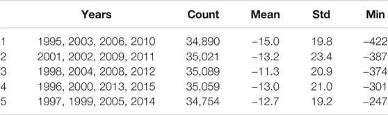
TABLE 1. Summary of the five subsets showing the years, number of samples, the mean (nT), standard deviation (nT), and minimum Dst (nT).
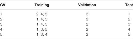
TABLE 2. Selection of subsets for the different cross-validation (CV) sets.
The input and target values span very different numerical ranges, whereas the training algorithm should receive input-target data that have similar numerical ranges. Therefore, the input and target data are normalized, where the normalization coefficients are found from the training set. By subtracting the mean and dividing with the standard deviation for each variable separately, the training set will have zero mean and one standard deviation on all its inputs and target variables. However, as the distributions for each variable are highly skewed, they result in several normalized values with magnitudes much larger than one. Another way to normalize is to instead rescale the minimum and maximum values to the range [-1, 1]. This guarantees that there will be no values outside this range for the training set. We found that the min–max normalization gave slightly better results, especially at the large values.
2.3 Hyperparameters
There are a number of hyperparameters (HPs) that control the model complexity and training algorithm that need to be tuned, but it is not feasible to make an exhaustive search. Initially, a number of different combinations of HP values were manually tested to provide a basic insight into reasonable choices and how the training and validation MSEs vary with epochs. In this initial exploration, we found the Tensorboard (Abadi et al., 2015) software valuable in monitoring the MSE.
The Adam learning algorithm (Kingma and Lei, 2015), which is a stochastic gradient descent method, has three parameters: learning rate ϵ and two decay rates for the moment estimates
The learning algorithm updates the weights in batches of samples from the training set, where the number of samples in each batch
The model capacity is determined by the number of weights and the network architecture. In this work, we have one input layer, a recurrent layer (hidden layer), and a single output. Thus, the capacity is determined by the network type
The current state
The dropout is controlled by parameters that specify the fraction of network units in a layer that are randomly selected per epoch and temporarily disregarded. The dropout can be applied to all layers: the input layer
For each combination of HP that we explore, we train three networks initiated with different random weight values as there is no guarantee that the training algorithm will find a good local minimum. The network with the lowest validation error is selected. Note that here validation refers to the split into training and validation sets used during training, which is different from the cross-validation sets that make up the independent test set.
2.4 Training Network on Simulated Data
It is interesting to study the RNNs on data generated from a known function relating solar wind to Dst, and for this purpose, we use the AK1 model (O’Brien and McPherron, 2000). Using the datasets defined in the previous section, we apply the AK1 model to the solar wind inputs and create the target data. Thus, there exists an exact relation between input and output, and the learning process of the RNN will only be limited by the amount of data, network structure (type of RNNs), and network capacity (size of RNNs). We showed that the minimalistic Elman network (Eq. 7) can model the pressure-corrected Dst. The AK1 model also includes the pressure term, and its inputs are
In Figure 1, the validation errors as function of T are shown for the Elman and GRU networks. At each T, the optimal networks with respect to
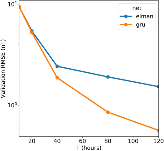
FIGURE 1. The average validation RMSE as function of memory size (T in hours) for the Elman and GRU networks.
2.5 Result for the Dst Index
As described in Section 2.2, the inputs to the Dst model are solar wind magnetic field
We perform a search in the hyperparameter space as described above and conclude that training is not very sensitive on the learning rate (ϵ) or batch size
For each of the five splits, we select the corresponding training set (Tables 1,2), and RNNs are trained with different number of hidden units
The coupling function from solar wind to observed Dst is subject to a number of uncertainties, and to provide a few examples: the solar wind data have been measured at different locations upstream of Earth, mostly from orbit around the L1 location, and then shifted to a common location closer to Earth (King and Papitashvili, 2005); We rely on a point measurement; there may be both systematic and random errors in the derived Dst index. The uncertainties introduce errors in the input–output mapping, and to reduce their effect and improve generalization, we apply dropout. From a search of different combinations of
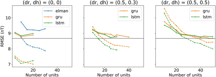
FIGURE 2. The average training (dashed lines) and validation (solid lines) RMSE as function of the number of hidden units (
For each CV set, we select the GRU and LSTM networks with minimum validation RMSE with and without dropout, and run them and collect the 5 CV sets into one set. We thereby get an estimate of the generalization performance for the whole 1995 to 2015 period. Figure 3 shows scatterplots of predicted Dst vs. observed Dst on the test sets for different networks. Table 3 summarizes the performance on the training, validation, and test sets. The 95% confidence intervals have been estimated by both assuming independent data points and taking into account the autocorrelation (Zwiers and von Storch, 1995). It is clear that using dropout significantly improves the generalization capability. We also see that there is no significant difference between the GRU and LSTM networks. The bias (mean of errors) and linear correlation coefficient are computed on the test set and shown in Table 4.
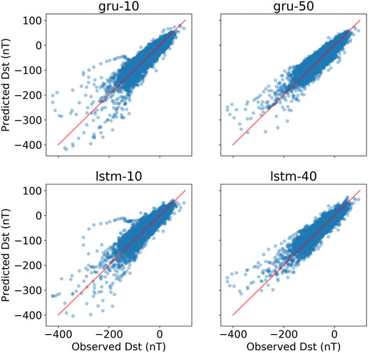
FIGURE 3. Scatterplots of predicted vs. observed Dst based on the five CV test sets. The left panels show predictions without dropout using GRU and LSTM networks (gru-10 and lstm-10), while the right panels are predictions based on networks trained using dropout of
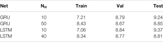
TABLE 3. Training, validation, and test RMSE (nT) for networks with and without dropout. The training and validation RMSE are averages over the five CV splits, while the test RMSE is computed from the combined five CV test sets. Networks with
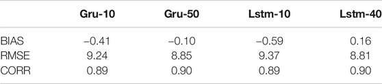
TABLE 4. BIAS, RMSE, and CORR for the GRU and LSTM models on the test set. BIAS and RMSE are in units of nT. The 95% confidence intervals are
The performance of the networks varies with the level of Dst; the errors have a tendency to increase with the magnitude of Dst. Figure 4 shows the RMSE binned by observed Dst. Down to
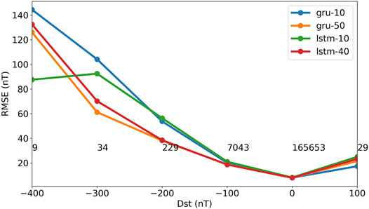
FIGURE 4. The test RMSE binned by observed Dst. The RMSE is computed on the five CV test sets. Bins are 100 nT wide, and the numbers show the number of samples in each bin. Legend: GRU (gru-10) and LSTM (lstm-10) networks without dropout, and GRU (gru-50) and LSTM (lstm-40) networks with dropout
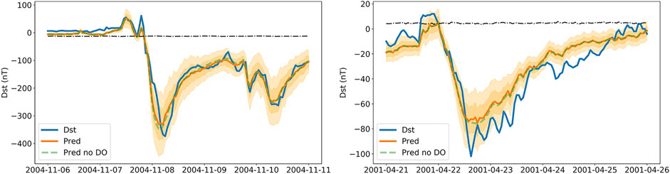
FIGURE 5. Two geomagnetic storms predicted with the GRU network using the test set. Panels show observed Dst (blue solid), predicted Dst without dropout during prediction phase (dashed green), and mean prediction with dropout (orange solid). The dark orange regions show the predicted
As time of day and season are included in the inputs, the network can model diurnal and seasonal variations in Dst. These variations are not strong, and the left panel in Figure 6 shows Dst for all years averaged over month and UT hour. Running the GRU networks on the test data from the five CV sets reveals a very similar pattern (second panel from left). Thus, the network shows similar long-term statistics considering that it is driven only by solar wind and time information. The two left panels contain contributions from all levels of Dst from quiet conditions to storm conditions. But we may now simulate solar wind conditions that we can define as quiet conditions. The two right panels show predicted Dst, assuming solar wind flowing out from the Sun (GSEQ system) along the Parker spiral with a
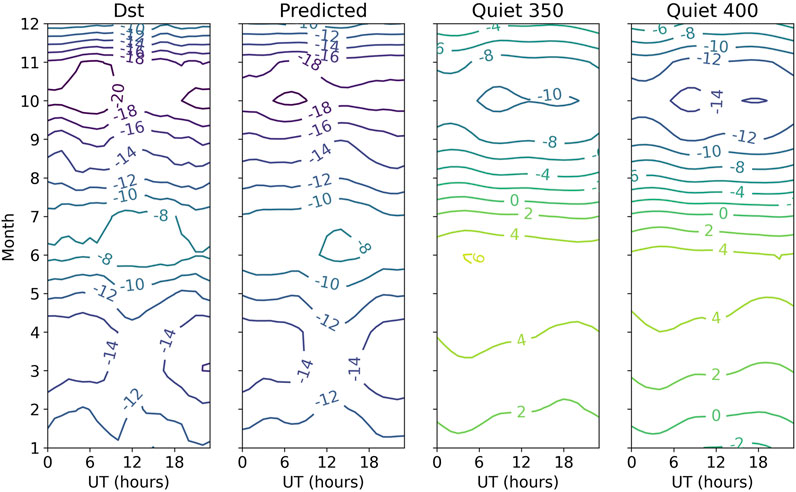
FIGURE 6. The panels show average Dst binned by month and UT hour. From left to right, the averages are based on all observed Dst (Dst), predicted Dst from the CV test sets (Predicted), predicted Dst from quiet solar wind at 350 km/s (Quiet 350), and predicted Dst from quiet solar wind at 400 km/s (Quiet 400) (see text for definition of quiet solar wind).
3 Discussion and Conclusion
There is a close correspondence between Elman networks and models expressed in terms of the differential equation for the Dst index. A minimalistic Elman network trained on simulated data from the pressure-corrected Dst index (Eq. 1) results in weights that translate to values around
The GRU (Cho et al., 2014) and LSTM (Hochreiter and Schmidhuber, 1997) networks include gating units that control information flow through time. However, it is not clear if one architecture is better than the other (Chung et al., 2014). In order to reliably study the differences between the two RNNs, we applied five-fold cross-validation. Further, it was also essential to apply dropout (Gal and Ghahramani, 2016) to reduce over-fitting and achieve consistent results. Using solar wind data and observed Dst from 1995 to 2015, we see no significant difference between the two architectures. However, the GRU network is slightly less complex than the LSTM and will therefore have shorter training times.
An interesting effect of using dropout is that it can also be applied during the prediction phase as a way of capturing model uncertainty (Gal and Ghahramani, 2016b). Using dropout during prediction is similar to ensemble prediction based on a collection of networks with identical architectures but different specific weights (Wintoft et al., 2017), but with the great advantage that the predictions can be based on, in principle, unlimited number of models. However, it is different from using an ensemble of different types of models like in Xu et al. (2020). We illustrated the prediction uncertainty using dropout for a couple of storms from the test set. Estimating the prediction uncertainty is important and was addressed by Gruet et al. (2018) using a combination of LSTM network and a Gaussian process (GP) model. In that case, the LSTM network provides the mean function to the GP model from which a distribution of prediction can be made. For future work, it will be interesting to further study the use of dropout for estimating model uncertainty.
Predictions based on the test sets using the GRU networks show very good agreement with observed Dst when averaged over month and UT (Figure 6). The semiannual variation (Lockwood et al., 2020) is clear, with a deeper minimum in autumn than in spring and a weak UT variation. It is a combination of geometrical effects that cause the asymmetric semiannual variation leading to a modulation of the
Data Availability Statement
Publicly available datasets were analyzed in this study. These data can be found here: https://omniweb.gsfc.nasa.gov/ow.html.
Author Contributions
PW and MW have carried out this work with main contribution from PW.
Conflict of Interest
The authors declare that the research was conducted in the absence of any commercial or financial relationships that could be construed as a potential conflict of interest.
Acknowledgments
We acknowledge the use of NASA/GSFC’s Space Physics Data Facility’s OMNIWeb (or CDAWeb or ftp) service and OMNI data.
Footnotes
1https://www.drivendata.org/competitions/73/noaa-magnetic-forecasting/page/278/
2https://github.com/spacedr/dst_rnn
Appendix: software and hardware
The code has been written in Python where we rely on several software packages: Pandas for data analysis (T. pandas-dev/pandas: Pandas, 2020); Matplotlib for plotting (Hunter, 2007); and TensorFlow and TensorBoard for RNN training (Dataset] Abadi et al., 2015).
The simulations have been run on an Intel Core i9-7960X CPU at 4.2 GHz with 64 GB memory. In total, 32 threads can be run in parallel. Typical training time for one Elman network with 30 hidden units for 50 epochs ranges between 5 and 15 min, where the shorter time is due to that the process could be distributed on multiple threads. We noted that one training process could be distributed over four threads, when the overall load was low. A GRU network with 10 hidden units could take between 30 min and slightly more than 1 h for 50 epochs. A 10-hidden unit LSTM network ranged between 50 min and 1.5 h.
References
Abadi, M., Agarwal, A., Barham, P., Brevdo, E., Chen, Z., Citro, C., et al. (2015). TensorFlow: Large-Scale Machine Learning on Heterogeneous Systems. Software available from tensorflow.org.
Bengio, Y., Simard, P., and Frasconi, P. (1994). Learning Long-Term Dependencies with Gradient Descent Is Difficult. IEEE Trans. Neural Netw. 5 157–166. doi:10.1109/72.279181
Boaghe, O. M., Balikhin, M. A., Billings, S. A., and Alleyne, H. (2001). Identification of Nonlinear Processes in the Magnetospheric Dynamics and Forecasting of Dst Index. J. Geophys. Res. 106, 30047–30066. doi:10.1029/2000ja900162
Borovsky, J. E., and Birn, J. (2014). The Solar Wind Electric Field Does Not Control the Dayside Reconnection Rate. J. Geophys. Res. Space Phys. 119 751–760. doi:10.1002/2013JA019193
Boynton, R. J., Balikhin, M. A., Billings, S. A., Sharma, A. S., and Amariutei, O. A. (2011). Data Derived Narmax Dst Model. Ann. Geophys. 29 965–971. doi:10.5194/angeo-29-965-2011
Burton, R. K., McPherron, R. L., and Russell, C. T. (1975). An Empirical Relationship between Interplanetary Conditions andDst. J. Geophys. Res. 80 4204–4214. doi:10.1029/ja080i031p04204
Cho, K., van Merriënboer, B., Gulcehre, C., Bahdanau, D., Bougares, F., Schwenk, H., et al. (2014). “Learning Phrase Representations Using RNN Encoder–Decoder for Statistical Machine Translation,”in Proceedings of the Conference on Empirical Methods in Natural Language Processing (EMNLP) (Doha, Qatar: Association for Computational Linguistics) 1724–1734. doi:10.3115/v1/D14-1179
Chung, J., Gulcehre, C., Cho, K., and Bengio, Y. (2014). Empirical Evaluation of Gated Recurrent Neural Networks on Sequence Modeling. NIPS 2014 Workshop on Deep Learning, December 2014.
Cybenko, G. (1989). Approximation by Superposition of a Sigmoidal Function. Math. Control Signals, Syst. 2 303–314. doi:10.1007/bf02551274
Elman, J. L. (1990). Finding Structure in Time. Cogn. Sci. 14 179–211. doi:10.1207/s15516709cog1402_1
Gal, Y., and Ghahramani, Z. (2016a). “A Theoretically Grounded Application of Dropout in Recurrent Neural Networks,” in 30th Conference on Neural Information Processing Systems (Barcelona, Spain: NIPS).
Gal, Y., and Ghahramani, Z. (2016b). Dropout as a Bayesian Approximation: Representing Model Uncertainty in Deep Learning. Proceedings of the 33rd International Conference on Machine Learning, New York, NY, United States, 2016, (JMLR: W&CP), 48.
Gleisner, H., Lundstedt, H., and Wintoft, P. (1996). Predicting Geomagnetic Storms from Solar-Wind Data Using Time-Delay Neural Networks. Ann. Geophys. 14 679–686. doi:10.1007/s00585-996-0679-1
Gruet, M. A., Chandorkar, M., Sicard, A., and Camporeale, E. (2018). Multiple-hour-ahead Forecast of the Dst Index Using a Combination of Long Short-Term Memory Neural Network and Gaussian Process. Space Weather 16, 1882, 1896. doi:10.1029/2018SW001898
Hochreiter, S., and Schmidhuber, J. (1997). Long Short-Term Memory. Neural Comput. 9 1735–1780. doi:10.1162/neco.1997.9.8.1735
Hunter, J. D. (2007). Matplotlib: A 2d Graphics Environment. Comput. Sci. Eng. 9 90–95. doi:10.1109/MCSE.2007.55
King, J. H., and Papitashvili, N. E. (2005). Solar Wind Spatial Scales in and Comparisons of Hourly Wind and Ace Plasma and Magnetic Field Data. J. Geophys. Res. 110, A02104. doi:10.1029/2004JA010649
Kingma, D. P., and Lei, Ba. J. (2015). “Adam: A Method for Stochastic Optimization,” in The 3rd International Conference on Learning Representations (ICLR), arXiv:1412.6980.
Lockwood, M., Owens, M. J., Barnard, L. A., Haines, C., Scott, C. J., McWilliams, K. A., et al. (2020). Semi-annual, Annual and Universal Time Variations in the Magnetosphere and in Geomagnetic Activity: 1. Geomagnetic Data. J. Space Weather Space Clim. 10 . doi:10.1051/swsc/2020023
Lundstedt, H., Gleisner, H., and Wintoft, P. (2002). Operational Forecasts of the geomagneticDstindex. Geophys. Res. Lett. 29, 34. doi:10.1029/2002GL016151
Lundstedt, H., and Wintoft, P. (1994). Prediction of Geomagnetic Storms from Solar Wind Data with the Use of a Neural Network. Ann. Geophys. 12, 19–24. doi:10.1007/s00585-994-0019-2
Mayaud, P. N. (1980). Derivation, Meaning, and Use of Geomagnetic Indices, Geophysical Monograph. 22 (American Geophysical Union.
O’Brien, T. P., and McPherron, R. L. (2000). Forecasting the Ring Current Dst in Real Time. J. Atmos. Solar-Terrestrial Phys. 62 1295–1299.
O’Brien, T. P., and McPherron, R. L. (2002). Seasonal and Diurnal Variation of Dst Dynamics. J. Geophys. Res. 107, 1341. doi:10.1029/2002JA009435
Pallocchia, G., Amata, E., Consolini, G., Marcucci, M. F., and Bertello, I. (2006). Geomagnetic Dst Index Forecast Based on IMF Data Only. Ann. Geophys. 24, 989–999. doi:10.5194/angeo-24-989-2006
Srivastava, N., Hinton, G., Krizhevsky, A., Sutskever, I., and Salakhutdinov, R. 2014). Dropout: a Simple Way to Prevent Neural Networks from Overfitting. J. Machine Learn. Res. 15, 1929–1958.
Tan, Y., Hu, Q., Wang, Z., and Zhong, Q. (2018). Geomagnetic Index Kp Forecasting with Lstm. Space Weather 16, 406–416. doi:10.1002/2017SW001764
Temerin, M., and Li, X. (2006). Dst Model for 1995–2002. J. Geophys. Res. 111, A04221. doi:10.1029/2005JA011257
Vassiliadis, D., Klimas, A. J., Valdivia, J. A., and Baker, D. N. (1999). The Dst Geomagnetic Response as Function of Storm Phase and Amplitude and the Solar Wind Electric Field. J. Geophys. Res. 104, 957–976. doi:10.1029/1999ja900185
Watanabe, S., Sagawa, E., Ohtaka, K., and Shimazu, H. (2002). Prediction of the Dst Index from Solar Wind Parameters by a Neural Network Method. Earth Planets Space 54, 1263–1275. doi:10.1186/bf03352454
Wintoft, P., and Wik, M. (2018). Evaluation of Kp and Dst Predictions Using Ace and Dscovr Solar Wind Data. Space Weather 16, 1972–1983. doi:10.1029/2018SW001994
Wintoft, P., Wik, M., Matzka, J., and Shprits, Y. (2017). Forecasting Kp from Solar Wind Data: Input Parameter Study Using 3-hour Averages and 3-hour Range Values. J. Space Weather Space Clim. 7, A29. doi:10.1051/swsc/2017027
Wu, J. G., and Lundstedt, H. (1997). Neural Network Modeling of Solar Wind-Magnetosphere Interaction. J. Geophys. Res. 102, 14457–14466. doi:10.1029/97ja01081
Xu, S. B., Huang, S. Y., Yuan, Z. G., Deng, X. H., and Jiang, K. (2020). Prediction of the Dst Index with Bagging Ensemble-Learning Algorithm. Astrophysical J. Suppl. Ser. 248. doi:10.3847/1538-4365/ab880e
Keywords: space weather, recurrent neural net, cross-validation, solar wind–magnetosphere–ionosphere coupling, prediction, dropout
Citation: Wintoft P and Wik M (2021) Exploring Three Recurrent Neural Network Architectures for Geomagnetic Predictions. Front. Astron. Space Sci. 8:664483. doi: 10.3389/fspas.2021.664483
Received: 05 February 2021; Accepted: 22 April 2021;
Published: 12 May 2021.
Edited by:
Enrico Camporeale, University of Colorado Boulder, United StatesReviewed by:
Jannis Teunissen, Centrum Wiskunde and Informatica, NetherlandsShiyong Huang, Wuhan University, China
Copyright © 2021 Wintoft and Wik. This is an open-access article distributed under the terms of the Creative Commons Attribution License (CC BY). The use, distribution or reproduction in other forums is permitted, provided the original author(s) and the copyright owner(s) are credited and that the original publication in this journal is cited, in accordance with accepted academic practice. No use, distribution or reproduction is permitted which does not comply with these terms.
*Correspondence: Peter Wintoft, cGV0ZXJAbHVuZC5pcmYuc2U=