Exploiting White-Light Observations to Improve Estimates of Magnetic Connectivity

1 Introduction

A new era in heliophysics has begun with the recent launches of the Solar Orbiter (SolO) and Parker Solar Probe (PSP) missions. The comprehensive instrumentation onboard these spacecraft and their proximity to the Sun will allow for detailed investigations of the relation between the solar wind properties measured in situ (IS) and their solar source regions observed by remote-sensing (RS) instruments. This IS-RS connection is typically established by considering magnetic field lines that connect to the same solar wind source region at the Sun. They can also act to channel energetic particles. Whichever the chosen model, Magneto-Hydro-Dynamic (MHD) or Potential Field Source Surface (PFSS) models, a common critical parameter is the input photospheric magnetic field map. Many magnetograms are now made available to the scientific community and can serve as the initial magnetic boundary condition for solar wind simulations. Some of them not only offer a single set but an ensemble of possibilities such as those computed by the Air Force Data Assimilative Photospheric Flux Transport (ADAPT) model, (see e.g. Arge et al., 2010; Arge et al., 2013). The ADAPT maps are global magnetograms of the photospheric magnetic flux and are produced using data assimilation techniques along with a magnetic flux transport model (see Worden and Harvey, 2000). Each ADAPT map has different realizations of the status of the photospheric magnetic field at a certain time. Selecting among so many magnetograms is a challenging task that is often done arbitrarily. In this work, we present a novel technique that it is designed to automatically test the reliability of the different realizations of the ADAPT maps. The developed method is based on a comparison of the global models of the solar atmosphere with the location of streamers in synoptic maps from white-light (WL) observations. The method is versatile by allowing us to perform such comparisons using any magnetograms and any type of global models.

The convenience of Carrington maps derived from WL observations has been demonstrated in many studies. Some of the earliest WL synoptic maps were constructed with K-corona images from the CORONASCOPE II and SOLWIND missions (Bohlin, 1970; Wang and Sheeley, 1992), as well as from the Mauna Loa Solar Observatory in Hawaï (Hansen et al., 1976). Later on, synoptic observations from the (WL) coronagraph onboard Skylab have been exploited to model the large scale coronal density structures by assuming that the peaks in brightness mark the location of the heliospheric current sheet (HCS) (Guhathakurta et al., 1996). The continuous monitoring of the solar corona by the Solar and Heliospheric Observatory (SoHO) has then enabled a more systematic comparison between the location of streamers with the magnetic topology of the solar corona derived from PFSS calculations (Wang et al., 1998; Wang et al., 2000; Wang et al., 2007) and global coronal models (Gibson et al., 2003; Thernisien and Howard, 2006; de Patoul et al., 2015; Pinto and Rouillard, 2017). Rotational tomography techniques have been developed recently to correct for line of sight effects and convert WL observations into synoptic density maps (Morgan and Cook, 2020). Other techniques have involved the combination of coronagraph images obtained from multiple vantage points, (e.g. SoHO and STEREO) simultaneously to derive synchronic circumsolar maps of helmet streamers (Sasso et al., 2019). WL Carrington maps have also been exploited to track the origin of the solar wind measured in situ at PSP (see e.g., Rouillard et al., 2020a; Rouillard et al., 2020c; Griton et al., 2021) or to study the fine structure of coronal rays observed remotely at PSP (see Poirier et al., 2020). The deflection of streamers during solar storms can also be investigated using WL Carrington maps (see e.g., Kouloumvakos et al., 2020). The assumption in these comparisons is that the bright helmet streamers mark the location of the (HCS). We will make a similar assumption throughout this work and in particular we will test its reliability in Section 3.

In Section 2, we show in detail the methodology followed to perform the systematic assessment of coronal models against WL observations. We exploit our automated detection of the streamer belt (SB) to infer the distribution of magnetic sectors by assuming that the core of the SB hosts the HCS. In Section 3, we then directly compare the sector structure inferred at the Sun with the one measured in situ by two space-based observatories orbiting one AU. Finally, in Sections 4, 5 we highlight the successes and also discuss the limitations of our automated technique for several practical applications for space weather related topics. We also discuss a connection with PSP and SolO observations.

2 Data and Methods

In this section we present the technique developed to compare coronal models against WL observations using an automated and systematic approach. We start with a description of the methods used to pre-process the coronagraph images (sub Section 2.1) and to construct the WL synoptic maps (sub Section 2.2). In sub Section 2.3 we present a technique used to identify and characterize streamer signatures in WL synoptic maps. Finally, in sub Section 2.4 we define a metric that can be used to score coronal models against WL observations and we compare a coronal model with observations using a test case.

2.1 Pre-Processing the White-Light Images

In this study we exploit WL observations from the Large Angle and Spectrometric Coronagraph (LASCO) C2 (LC2) coronagraph on-board SoHO. SoHO is a collaborative ESA-NASA mission launched on December 2, 1995, and which is still operating at the Lagrange point L1. The SoHO spacecraft is equipped with an imaging suite composed of three coronagraphs (see Brueckner et al., 1995), two of which (namely the LASCO, C2, and C3) are still operating and observe continuously the corona in visible light. The LC2 coronagraph has a field-of-view (FOV) extending from $1.5R_{\odot }$ to $6R_{\odot }$ while LC3 has a much wider FOV extending to $30R_{\odot }$. In this study we exploit LC2 observations to build our model, but the methods we will present can also be applied to LC3 observations. We note, however, that the application of our technique to LC3 images would require further processing in order to derive a useful mapping of helmet streamers.

The WL emission observed by the coronagraphs comes from several distinct contributions. The dominant one comes from the photospheric light that is scattered by dust particles; this forms the F-corona. Dust particles are ubiquitous around the Sun but a number of theoretical studies predict the presence of a “dust-free” zone (see e.g., Lamy, 1974; Mukai et al., 1974), which might have been detected for the first time by the Wide-field Imager for Solar PRobe (WISPR) onboard PSP (see Howard et al., 2019). Another contribution is the photospheric light scattered by coronal electrons; this forms the so-called K-corona that is of interest for this study. WL images of the K-corona can help to locate streamers and streamer rays, where a subset of the slow solar wind forms. The brightest signatures in WL images come from regions of dense plasma such as the streamers.

Coronagraphic images must be processed beforehand to remove the F-corona. An estimate of the F-corona brightness distribution is derived by considering LC2 images over several days to a month, this image is then subtracted from the raw image to reveal the fine details of the K-corona. This technique has been used for several decades and is adequate for spacecraft moving slowly along their orbit such as SoHO located at one AU. It is however no longer suitable for fast-moving observatories such as WISPR onboard PSP, requiring more sophisticated techniques (see Stenborg et al., 2018; Hess et al., 2020). For SoHO LASCO we exploit the “monthly min” background images that are provided through https://sohowww.nascom.nasa.gov/.

In Figure 1 we show an example of a processed LASCO C2 image on the 2020/10/03 at 12:00. This image reveals the K-corona composed on that day of two large streamer rays one off the East (left) and West (right) limbs. These streamer rays emanate from the tip of helmet streamers and extend to the high corona.

FIGURE 1

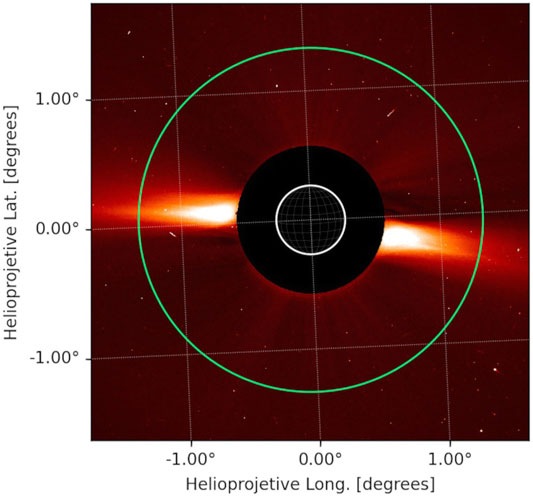
FIGURE 1. A processed LASCO C2 image on the 2020-10-03 at 12:00. The green circle depicts the band of pixels that are extracted at $5.0R_{\odot }$ at both East and West limbs to build the synoptic map afterward.

2.2 Construction of the White-Light Synoptic Maps

To visualize the complete SB we construct a synoptic map given in a heliographic latitude vs. Carrington longitude format by considering LC2 images obtained over a complete solar rotation. The SB is the name given to the 3-D shape formed by streamer rays over the full solar rotation. Each LC2 image is first projected onto the helioprojective sphere, which is defined as the sphere of radius the Sun—observer distance and with the observer at its center. Once a coordinate is associated to each image pixel, a band of pixels of circular shape is extracted from each image at a specific heliocentric radial distance (green line in Figure 1), which will be called hereafter the height of the Carrington map. After a coordinate transformation into the Carrington frame, the extracted pixels are mapped onto a latitude vs. longitude map (green line in Figure 2). As images are concatenated over time, pixels fill up the synoptic map until the latter covers a full solar rotation. The full synoptic map can then be continually updated as new images become available, thus providing a dynamic synoptic map.

FIGURE 2

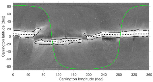
FIGURE 2. White-light synoptic (or Carrington) map at a height of $5R_{\odot }$ built after concatenating LASCO C2 images from 2020–09–19 12:00 to 2020–10–03 12:00. The green line represents the bands of pixels from the LASCO C2 image shown in Figure 1 that have been projected into the synoptic map. The SB contour and SMB line are drawn as dark solid and dashed lines, respectively (they are introduced in sub section 2.3).

The height at which pixels are extracted from the images plays a significant role into building a synoptic map. A height too close to the inner edge of the coronagraph would give a signal that is too saturated, whereas WL features are not so well resolved near the outer edge. Furthermore, streamer rays get narrower with increasing heliocentric distance, resulting in a change of the SB thickness in synoptic maps. A synoptic map with a SB that does not evolve anymore with increasing height is therefore preferred. This condition is usually satisfied at a height greater than $4R_{\odot }$, where most of the coronal magnetic field becomes radial as seen in eclipse images by Boe et al. (2020).

Although WL synoptic maps such as Carrington maps have been widely used in the past, their interpretation can be tricky. Relating bright WL signatures to dense coronal structures is not trivial. The major difficulty arises from the fact that a WL detector integrates light emitted from a range of locations extending along the line-of-sight. This induces some uncertainty in associating specific structures modeled in 3-D, such as streamers, with their WL signature. The combined effects of the inverse square falloff with heliocentric radial distance, of both the solar wind density and of the photospheric light intensity, mean that most of the WL contribution is expected to come from electrons located near the “Thomson sphere” (e.g. Vourlidas and Howard, 2006; Howard and Tappin, 2009). This sphere is geometrically defined as a sphere of diameter, the Sun—observer distance, and whose center is located at half this distance. A later study from Howard and DeForest (2012) showed that contributions to the total brightness are actually distributed over a broader region called the “Thomson plateau”, with the “Thomson sphere” standing in the middle. A recent study by Morgan and Cook (2020) tackled this line-of-sight integration problem by using rotational tomography which exploits the Sun’s rotation to resolve spatial density structures. This is a highly sophisticated method that requires additional modeling assumptions. We do not exploit such a method in order to keep our automated technique purely based on WL observations without any additional modeling aspects. We are aware of these line-of-sight related uncertainties, which are expected to occur mostly at places of large folds in the SB and mainly in the longitudinal direction.

The WL synoptic map shown in Figure 2 depicts a coronal configuration typical of a low solar activity, with a SB that remains flat most of the time. Only a small folding of the SB can be seen at 70 deg Carrington longitude along with a drift away of the SB toward higher latitudes. PFSS reconstructions of the coronal magnetic field suggest that, in this case, this bright excursion is part of an arch from a pseudo-streamer. But other inverted arch features, called “bananas” in Gibson et al. (2003), can also be observed in WL synoptic maps from the projection of non-equatorial streamers due to coronal rotation (see also Wang and Sheeley, 1992; Wang et al., 2000; Wang et al., 2007). These projection effects are particularly accentuated for observatories that are located much closer to the Sun such as WISPR onboard PSP (see e.g., Liewer et al., 2019; Poirier et al., 2020).

2.3 Identifying the Features of Interest in Synoptic Maps

Our aim is to exploit WL observations to determine if the HCS derived by a particular magnetic model of the solar atmosphere reproduces the position of bipolar streamers well. Therefore, our algorithm relies on the clear identification of coronal rays that originate from the tip of bipolar streamers. However, coronal rays observed in coronagraph images can have other origins. For instance they can emanate from other types of streamers called pseudo-streamers, which are particularly common during high solar activity. In contrast to bipolar streamers, pseudo-streamers form in open field regions of the same polarity and therefore cannot be related to the origin of the HCS of interest here. Fortunately, streamers and pseudo-streamers usually have different radial extensions in the corona, and there can be used to discriminate between the two. Pseudo-streamers are expected to be smaller structures compared to streamers, with a cusp located lower in the corona than bipolar streamers (Wang et al., 2007). We have found that at a heliocentric distance of $2.5R_{\odot }$ both pseudo-streamers and bipolar streamer rays tend to be equally bright whereas higher up near $5R_{\odot }$ coronal rays from pseudo-streamers appear dimmer in comparison with bipolar streamer rays which remain clearly visible. As a consequence, in the remaining of the paper we exploit LASCO C2 synoptic maps constructed at $5R_{\odot }$.

We also apply a 2-D median filter to reduce the effects of “hot pixels” and small artifacts related, (e.g. remaining cosmic rays), to ease the automatic identification and tracing of the SB. This tracing is performed by using a specific brightness threshold value (dark solid line in Figure 2). During the building process of the WL map, a dynamic scaling of the brightness is performed. Brightness is normalized by the maximal value of the current band of pixels that is extracted from the image. A single threshold value can therefore be set up to trace the SB contour in a consistent manner over the full solar rotation. Another advantage is that it allows a coherent scientific interpretation since the maximal brightness is likely to take place around the HCS.

The SB identification can be compromised in certain regions where WL emissions from the SB become faint as seen near longitudes 60° and 200° in Figure 2. This dimming happens when solar rotation brings the local tangent plane to the belt at high angles to the line of sight of the observer. Indeed, when the angle between the plane’s normal vector and the line of sight decreases, the section of the belt scattering photons back to the observer becomes much smaller. This effect becomes very common when the Sun gets more active with a dominant quadrupolar structure and the belt undergoes significant latitudinal excursions. In such configurations, the SB appears no longer continuous but rather fragmented, visible as separate SB bands in Carrington maps. These regions of large folding are difficult to address in an automated manner and they are consequently removed from the comparison with the models.

As discussed earlier, coronal rays from streamers are expected to be a good proxy to visualize where solar magnetic field reversals take place in the outer corona and inner heliosphere. The SB identified above already outlines the region where we expect those reversals. But we can go further by assuming that magnetic polarity changes are likely to occur where the plasma is densest within the core of the SB, and hence where the streamer total brightness reaches a maximum. Indeed, the HCS is usually measured in situ during the passage of the thin Heliospheric Plasma Sheet (HPS), a region of the solar wind that is usually associated with an order of magnitude increase in density (Winterhalter et al., 1994). The thickness of the HPS measured in situ tends to be thinner than streamers; the first WISPR images taken by PSP suggest that the HPS is a smaller but very bright region of the streamer located right at its core (Poirier et al., 2020; Rouillard et al., 2020c). An algorithm was therefore set up to trace the line passing through all the peaks of total brightness. This line covers a full solar rotation and is hereafter called the Streamer-Maximum-Brightness (SMB) line (dark dashed line in Figure 2). In Section 3, we will show a very good agreement between the estimated times when spacecraft are expected to cross the SMB and the crossings of HCS detected in situ.

2.4 Defining a Metric to Compare the Coronal Models With Observations

The technique presented in this paper aims to evaluate global coronal models against WL observations in an automated and systematic manner. For this purpose one needs to define a metric, a single quantity that evaluates how well the models agree with the WL observations. We define a metric that is comprehensive and which aims to compare distinct models to each other. We will illustrate the final metric by applying our automated technique to several extrapolations produced by a PFSS model. We choose a PFSS model rather than MHD models for simplicity, but the automated technique is applicable to any other types of models such as full 3-D MHD as long as they provide the location of the HCS (see e.g. Badman et al., 2021).

The position of the neutral line (NL) is therefore a necessary input from the model to be evaluated. For a PFSS model, the NL location is obtained at the outer boundary of the extrapolation domain, which is the source surface where magnetic field lines are assumed to be radial and open into the interplanetary medium. The height of this source surface is generally $2.5R_{\odot }$ from the Sun’s center but as we will see the present technique can be used to decide an optimal source surface height $\left({\text{R}}_{\text{ss}}\right)$. Beyond the source surface the magnetic field is assumed to be fully radial. Since the SMB is derived from LC2 at $5R_{\odot }$ we can simply project the PFSS neutral line radially outward from 2.5 to $5R_{\odot }$ for comparison purposes.

Angular distances between the model NL and the SMB line are calculated for a maximum of 180 points along the streamer belt. The SB contour is then exploited in order to normalize these angular distances by the observed thickness of the streamer. In regions where the outline of the SB is not clearly determined, usually due to large folds (see sub Section 2.2), the normalized angular distances are not computed. This ensures that uncertain regions where the SMB is poorly observed do not affect the final result.

The next step is to combine the modeled NL—SB angular distances derived over 360 degrees of longitude into a global score that tells us how well the model NL matches the SB location. A mean value $\left(\overline{\alpha }\right)$ is computed over all local angular distances using the following formula:

$\overline{\alpha }=\frac{1}{n}{\displaystyle \sum _{i=1}^n\widetilde{{\alpha }_i}}\text{and}\widetilde{{\alpha }_i}=\frac{\left|{\alpha }_i\right|}{T_i},(1)$

where ${\alpha }_i$ is the local angular distance between the SMB and the model NL, $T_i$ is the local streamer angular thickness and n is the number of $T_i$ values that could be measured. The lower the mean value $\overline{\alpha }$, the higher the match between SMB and model NL. A mean value $\overline{\alpha }=0$ would be indicative of a modeled NL that perfectly matches the SMB location. A mean value $\overline{\alpha }=1$ would depict a NL that is more distant from the SMB line but remaining in average at the edges of the SB. Finally a mean value $\overline{\alpha }>1.5$ would point out a NL that is significantly inconsistent with the white-light observations.

In addition to the mean value $\overline{\alpha }$, the standard deviation is calculated to assess the data dispersion. We are mostly interested in the data dispersion above the mean, which is representative of large distances to the SMB line. Hence the standard deviation is computed among the values that are greater than the mean value only:

${\sigma }_{+}=\sqrt{\frac{1}{n_{+}}{\displaystyle \sum _{i=1}^{n_{+}}{\left(\widetilde{{\alpha }_i}-\overline{\alpha }\right)}^2}},(2)$

where $n_{+}$ is the number of local values $\widetilde{{\alpha }_i}$ that are greater than the mean value $\overline{\alpha }$.

A final parameter called the confidence score, C, is computed by combining both $\overline{\alpha }$ and ${\sigma }_{+}$ parameters. For convenience, the confidence score is transformed into a percentage between 0 and 100%. The higher the percentage, the closer the match between the NL and the SMB. Two sigmoid functions are used to perform this transformation, hereafter called gain $g\left(\overline{\alpha }\right)$ and penalty $p\left({\sigma }_{+}\right)$ function. The final confidence score is the result of a gain score to which a penalty score is subtracted as follows:

$\begin{array}{l}C\left(\overline{\alpha },{\sigma }_{+}\right)=g\left(\overline{\alpha }\right)\times \left[1-p\left({\sigma }_{+}\right)\right],\\ g\left(\overline{\alpha }\right)=\frac{1}{1+{\left(99\right)}^{\overline{\alpha }-1}},\\ p\left({\sigma }_{+}\right)=\frac{1}{1+{\left(\frac{1}{99}\right)}^{{\sigma }_{+}-1}}.\end{array}(3)$

The gain function has been designed so that a mean value $\overline{\alpha }=1$ (and $\overline{\alpha }=2$) leads to a gain score of 50 (and 1%). In a similar manner, the penalty function has been set so that a dispersion coefficient ${\sigma }_{+}=1$ (and ${\sigma }_{+}=2$) gives a penalty score of 50 (and 99%).

In Figure 3 we compare several PFSS extrapolations against the SMB line and SB contour identified earlier in Figure 2. Results from the metric defined above are given in the legend including the mean score $\overline{\alpha }$ (Eq. 1), the dispersion coefficient ${\sigma }_{+}$ (Eq. 2) and confidence score C (Eq. 3). A PFSS model has been exploited here because it allows us to perform a quick benchmark analysis by testing our metric over a broad range of parameters. However, we emphasize that this metric can easily by applied to any other input magnetogram and to models other than PFSS. Cases 2 and 3 (plotted in yellow and purple color in Figure 3) are of interest because they have almost equal mean values $\overline{\alpha }$ but locally case 3 differs more extensively. Case 3 is hence penalized for having a higher dispersion coefficient ${\sigma }_{+}$ which is reflected in a confidence score of $16.5\text{\%}$, much lower than for case 2 with $38.9\text{\%}$. Case 1 depicts a model that is significantly inconsistent with WL observations whereas cases 5 and 4 are representative of models that match well with WL observations. For completeness, we provide in Figure 4 three graphs that illustrate how the confidence score (in percentage) is computed from the $\overline{\alpha }$ and ${\sigma }_{+}$ parameters using the two sigmoid functions defined in Eq. 3. We labeled the five cases mentioned above in Figure 4. Panel (A) from Figure 4 displays all confidence scores that can be obtained from any pair of ($\overline{\alpha }$,${\sigma }_{+}$) parameters. Both $\overline{\alpha }$ and ${\sigma }_{+}$ parameters have an equivalent impact on the final confidence score so that a model having local and large discrepancies with WL observations will be penalized.

FIGURE 3

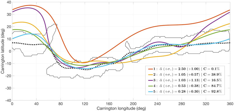
FIGURE 3. Comparison of several NLs against the SMB line and SB contour identified in Figure 2. NLs computed from the PFSS model using different ${\text{R}}_{\text{ss}}$ and magnetograms on the 03–10-2020 12:00 from: 1) GONG/mrbqs (${\text{R}}_{\text{ss}}$: $3.0R_{\odot }$); 2) GONG/ADAPT 7th realization (${\text{R}}_{\text{ss}}$: $2.5R_{\odot }$); 3) GONG/ADAPT 10th realization (${\text{R}}_{\text{ss}}$: $2.0R_{\odot }$); 4) GONG/ADAPT 10th realization (${\text{R}}_{\text{ss}}$: $3.0R_{\odot }$); and 5) GONG/mrzqs (${\text{R}}_{\text{ss}}$: $3.0R_{\odot }$). For each model the mean and dispersion values ($\overline{\alpha }$ and ${\sigma }_{+}$) are given in the legend as well as the associated confidence scores C (%) computed with Eq. 3.

FIGURE 4

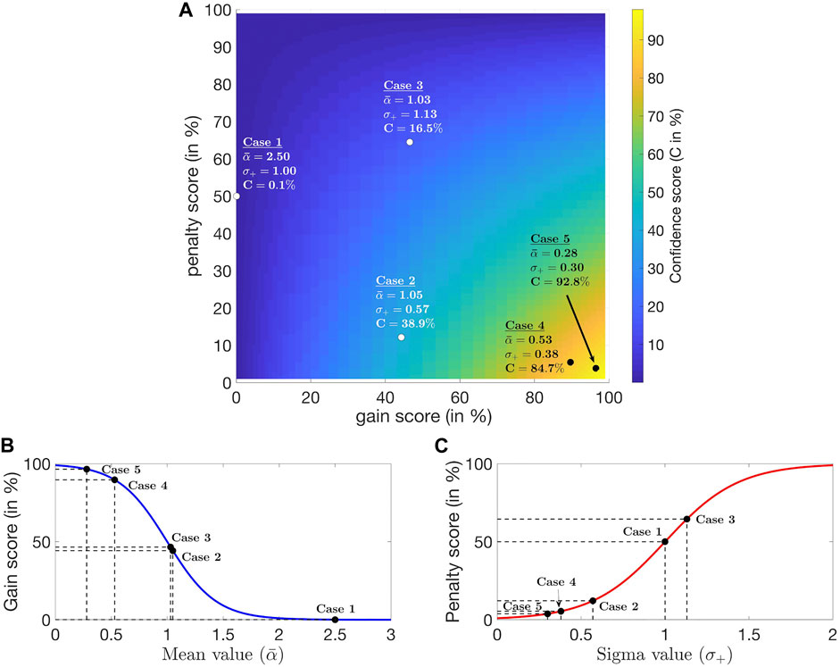
FIGURE 4. (A): 2-D colored map of confidence scores C as a function of both the gain and penalty scores. (B) and (C): gain and penalty scores as a function of the mean value $\overline{\alpha }$ and dispersion coefficient ${\sigma }_{+}$. All scores are given as percentages. The five cases already shown in Figure 3 are also annotated.

We illustrate our scoring technique in Figure 5. Confidence scores of multiple PFSS extrapolations can easily be compared with each other, allowing a quick selection of the PFSS model parameters that best fit the SB location on a specific date. In this example, the GONG/mrzqs (“ZGONG”) magnetogram with a RSS at $3.0R_{\odot }$ shows the best WL performance followed by the GONG/ADAPT 10th realization (“AGONG_10”) at $3.0R_{\odot }$. We also indicate in brighter shaded areas the impact of the dispersion coefficient ${\sigma }_{+}$ (via the penalty function $p\left({\sigma }_{+}\right)$) on the final confidence score. Two trends can be quickly observed in this example: the higher the ${\text{R}}_{\text{ss}}$, the better is the confidence score with a lower dispersion. A better match between the SB location and the NL for a source surface height of $3.0R_{\odot }$ rather than the typical $2.5R_{\odot }$ is consistent with the conclusions made by Boe et al. (2020) by exploiting many total solar eclipse images.

FIGURE 5

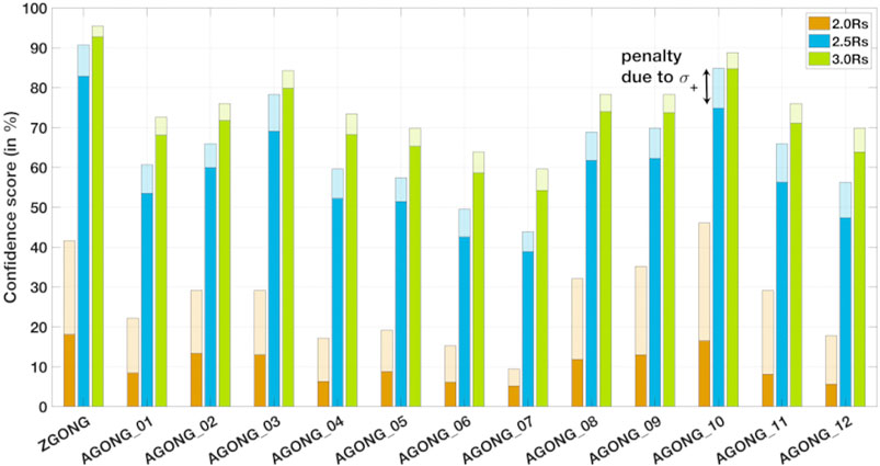
FIGURE 5. Summary plot of PFSS models performances according to WL, using GONG/mrzqs (labeled “ZGONG”) and GONG/ADAPT (labeled “AGONG_XX”) magnetograms and three distinct ${\text{R}}_{\text{ss}}$ of $2.0R_{\odot }$, $2.5R_{\odot }$, and $3.0R_{\odot }$. Bright shaded areas illustrate confidence scores that would be obtained without the penalty induced by the dispersion coefficient ${\sigma }_{+}$.

3 Correlation With Magnetic Sectors Measured in situ at One AU

As discussed above, the brightest WL emissions are likely associated with the very dense plasma located in the HPS that encloses the HCS. This assumption can be tested by connecting WL observations with direct in situ measurements of the magnetic sector structure. In the early 70 s, a strong correlation was already found between the brightest regions of the K-corona and the sector boundaries measured in situ at one AU (Hansen et al., 1974; Howard and Koomen, 1974). We check again this correlation by developing a method to assess in a statistical manner, the magnetic field reversals measured in situ vs. the SMB lines derived from the WL synoptic maps. We exploited one year of magnetic field measurements from the Advanced Composition Explorer (ACE) and the Solar TErrestrial RElations Observatory (STEREO-A).

A sector structure can be derived from the WL synoptic maps by assuming that the SMB line is the location of the neutral line at $5.0R_{\odot }$ and that during the period of weak solar activity investigated here the solar magnetic field is mostly dipolar. With this configuration and the current dipole axis of the Sun we expect that any region located north/south of the SMB will be of positive/negative polarity. We then assume that both ACE and STEREO-A spacecraft are magnetically connected to $5.0R_{\odot }$ by the nominal Parker spiral. This spiral is defined by using the solar wind bulk velocity measured in situ at ACE and STEREO-A. The resulting footpoints at $5.0R_{\odot }$ can then be directly compared with respect to the SMB line. The magnetic polarities of the field lines connected to ACE and STEREO-A are then determined by assigning a positive/negative polarity depending on whether the footpoints are located north or south of the SMB line.

WL-derived magnetic sector maps can then be compared to sectors measured directly in situ. In order to compare one year of data in a convenient way we bin the data in Bartels map format. Such maps are shown in Figure 6 for STEREO-A [panels (A) and (C)] and ACE [panels (B) and (D)]. They have been constructed using 16-h averaged in situ measurements [panels (C) and (D)] and WL observations [panels (A) and (B)]. Bartels maps display successive Carrington rotations along the ordinate, and time during a specific rotation along the x axis (here the Carrington longitude). With a Solar rotation period of 27.27 days as viewed from Earth (synodic period), the map is progressively filled up from right to left and from top to bottom. Bartels maps are useful to visualize at a glance magnetic sectors and their variability over consecutive Carrington rotations.

FIGURE 6

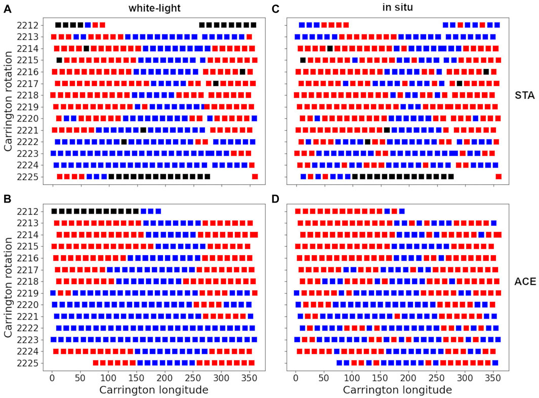
FIGURE 6. Bartel’s diagrams constructed with the SMB lines from the WL observations, for STEREO-A (A) and ACE(B). Bartel’s diagrams using direct in situ polarity measurements taken over the full year 2019 at STEREO-A (C) and ACE(D). Blue and red colors indicate positive and negative polarities respectively (dark colors correspond to data gaps).

Data are color-coded in blue (and red) for positive (and negative) polarities. Figure 6 brings out a good correspondence between in situ and WL derived Bartel’s diagrams with very similar sector structures, with $76.5\text{\%}$ of matching polarities for STEREO-A and $77.3\text{\%}$ for ACE. This shows that, overall, the SMB location offers a good estimate of where polarity inversions should occur at the Sun and therefore the relevance of the presented technique to provide additional constraints to global coronal models.

4 Applications

The presented metric can be of interest for many direct applications. In this section we present preliminary works that illustrate several of these possibilities.

4.1 Understanding in Situ Measurements at PSP

Such a comparison can be repeated in the context of the SolO and PSP missions. Their proximity to the Sun offer the opportunity to probe in greater detail the relation between HCS crossings measured in situ and their origin in WL. Since those measurements have been taken in the heliosphere, a projection of these data back to the solar corona is needed. We use the same ballistic mapping as employed before, with the nominal Parker spiral extending from PSP down to the height of the WL synoptic map at $5.0R_{\odot }$ and defined by the solar wind speed measured by PSP. The locus of footpoints of the spiral connecting PSP to $5.0R_{\odot }$ can be plotted on the Carrington map and for each point we can assign the polarity of the magnetic field measured in situ by PSP. This is illustrated in Figure 7 where in situ magnetic measurements at PSP are plotted in blue (and red) for positive (and negative) polarity. An animated version of this Figure is available in the online material, providing a time-dependent comparison between the acquisition of data by PSP along its orbit and the updating of the WL Carrington map as new coronagraphic data becomes available. Regions where in situ magnetic reversals do not match exactly the location of the SMB are often resolved a few days later when the WL map has been updated locally. From a broader perspective Figure 7 also illustrates the relevance of WL synoptic maps to provide a context for understanding solar wind properties measured in situ at PSP, such as the electron density (see e.g. Rouillard et al., 2020c; Griton et al., 2021).

FIGURE 7

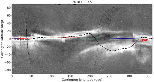
FIGURE 7. History of magnetic polarities measured in situ at PSP from 21-10-2018 to 04-12-2018. In the background a WL synoptic map from LASCO C2 at $5.0R_{\odot }$ and the SMB line as a dark dashed line are shown. A dynamic update of this figure over time is available in the online material, where the thick dot highlights the current in situ measurement on top of the past and future track. Positive (and negative) polarities are represented in blue (and red) colors.

4.2 Constraining PFSS Coronal Models in a Systematic Manner

PFSS coronal models usually set a source surface height at $2.5R_{\odot }$, from which the magnetic field is supposed to remain purely radial. However a recent study exploiting total solar eclipse images demonstrated that the solar magnetic field does not become radial below $3.0R_{\odot }$ at least (see Boe et al., 2020). They have also pointed out the fact that the source surface is likely not spherical as stated in other studies using PSP in situ data (see e.g., Badman et al., 2020; Panasenco et al., 2020). With some adjustments, the presented method could also provide constraints to PFSS models with a non-spherical source surface, allowing to optimize a longitudinally varying source surface height. By exploiting our technique over the first six PSP encounters (see Badman et al., 2021), we have found that generally PFSS models show a better agreement with the WL observations when assuming a ${\text{R}}_{\text{ss}}$ of $3.0R_{\odot }$. Two other metrics have also been exploited in Badman et al. (2021), one that is based on magnetic polarities measured in situ, and the other on the identification of coronal holes in EUV synoptic maps. These metrics tend to provide opposite optimum results for ${\text{R}}_{\text{ss}}$ by favoring PFSS models with lower ${\text{R}}_{\text{ss}}$.

4.3 Constraining MHD Simulations

One of the most critical parameters in any coronal or heliospheric model is the magnetogram used for the inner boundary of the simulated domain. Whatever the accuracy of the model, the magnetogram will have a major impact on the final outcome. The technique presented in this work can be used to select which combination of magnetograms and models provide the best modeling of the streamer belt. MHD models are more challenging to operate because more constraints are required compared to PFSS models. In addition to the magnetic field, one needs to set the plasma bulk properties at the inner boundary of the simulation domain. The well-known Wang-Sheeley-Arge (WSA) model established an empirical law to estimate the solar wind velocity based on the expansion factor of open magnetic field lines between the photosphere and the source surface (see Wang and Sheeley, 1990; Arge and Pizzo, 2000). We have recently exploited our SMB identification technique to derive an alternative empirical law relating the angular distance of a point situated anywhere on the Carrington map to the SMB, to the plasma density and velocity that we should expect. In situ measurements from the Ulysses, ACE and WIND missions have been exploited to build empirical laws for the solar wind density and velocity, function of the angular distance to the SMB, this will be presented in a future study. In this relation, regions situated close to the SMB will produce a slower and denser solar wind than regions located far from the SMB. Examples of such derived maps are given in Figure 8 and have been injected as solar wind density and velocity 2-D maps in MHD heliospheric simulations extending typically from 21.5 to 215 solar radii such as the ENLIL model (see Odstrcil, 2003). The inner boundary of the MHD simulation can then be updated on a, (e.g., daily) basis as new WL observations are available and the algorithm presented here updates the position of the SMB. Results on this topic are still preliminary and will be presented in a dedicated study. A major benefit of this method is that it allows to dynamically constrain heliospheric models, therefore improving forecast capabilities for space weather purposes.

FIGURE 8

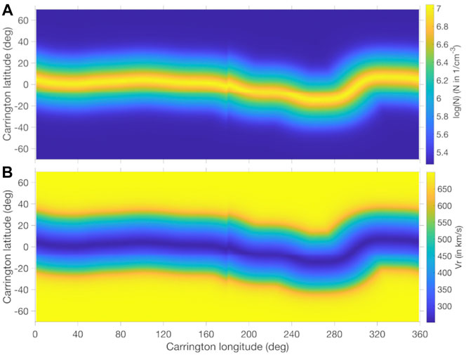
FIGURE 8. 2-D maps of solar wind density (A) and radial velocity (B) determined from the SMB line extracted on the 2019-06-15 at 12:00 UTC from LASCO-C2 WL observations at $5.0R_{\odot }$.

4.4 Improving Sun to S/C Connectivity Estimates

Coronal and heliospheric models are essential in the context of SolO and PSP science because they allow us to estimate the possible origins of the solar wind plasma measured in situ at those spacecraft or connect energetic particles to potential accelerators at the Sun, (e.g. flares, shocks). A web-based service tool has been put in place by the Solar Orbiter Data Analysis Working Group (MADAWG) to provide support to SolO operations (Rouillard et al., 2020b). This tool, called the Magnetic Connectivity Tool, is directly accessible to the public at this website¹. Forecast and past magnetic connectivities among many observatories such as PSP, SolO, BepiColombo, STEREO, and ACE are available via this web interface. Different magnetograms, coronal and heliospheric models can also be specified by the user. Recently, we implemented the technique presented in this paper to automatically select the combination of PFSS reconstructions—magnetograms that best fit WL observations to improve connectivity estimates. The selection is performed among several distinct sources of magnetograms such as those produced by the National Solar Observatory (NSO) and the Wilcox Solar Observatory (WSO), including those computed with the ADAPT model.

5 Limitations

The most critical step in the methodology presented in this work is having a correct identification of the SMB line. We have noticed several difficulties that can make this identification challenging and sometimes even produce erroneous estimates.

We especially pointed out cases where there are large folds in the SB. Since our method does not resolve the line-of-sight (as in tomographical approaches), our metric can not give an accurate estimate of the HCS location where the SB is significantly warped. Nearby SB folds, inverted arches can also appear which result from the projection of non-equatorial streamer rays along the line-of-sight. Regions of large warping of the SB are in general omitted in our metric because their WL signature is too faint to be detected by the algorithm. However, we plan to incorporate an actual detection of SB folds so that they can be systematically removed from our metric.

Furthermore, highly structured coronal configurations that are typically observed during Solar maximum may require further adjustments of the identification technique, which has not yet been fully tested for those particular cases. Such extreme cases where a significant fraction of the SB is highly warped may affect the reliability of our metric.

In addition, the presence of pseudo-streamers can make the identification of the SMB ambiguous because they can be on occasion brighter than the bipolar streamers, especially in regions where the SB is warped. Distinguishing pseudo-streamers from bipolar streamers is therefore tricky. We found that lifting the height of the WL synoptic maps to $5.0R_{\odot }$ helps but does not solve the issue entirely. Increasing the height might be possible by further improving the post-processing of the WL images.

Another approach to separate pseudo-streamers from bipolar streamers could be designed by exploiting in situ measurements, as was done in Section 3 and in sub Section 4.1. A combination of our WL-based technique with a back-mapping of the sector structure measured in situ could be devised in an automated manner. It was attempted on a case by case basis by Badman et al. (2021) and showed some great potential. It can also provide a local assessment of the models and so diminish the impact of the global score provided by the WL-based approach. This is a possibility that we will attempt in the future.

Finally, another important point relates to the cadence with which WL Carrington maps are updated. We have found that discrepancies between the SMB line and the sector structure measured in situ from ACE, STEREO (see Section 3) or PSP (see sub Section 4.1) are often caused by the updating of the WL synoptic maps from off-limb observations. The rate of update in the map at a particular Carrington longitude and from a single viewpoint is set by the time a particular longitude rotates from the East to the West limb. From one AU this imposes an update every 14 days. This cadence can be greatly increased by combining coronagraphic observations from other vantage points than LASCO. This was the motivation for the development of merged synoptic maps from SoHO LASCO and STEREO SECCHI as performed by Sasso et al. (2019). Our next step is to incorporate these synchronic maps built from several vantage points.

6 Conclusion

We introduced a novel automated technique that provides an important constraint to coronal and heliospheric models based on the exploitation of WL observations. WL images from the LASCO C2 coronagraph are processed and converted into synoptic maps called Carrington maps, which are dynamically updated as new images are available. Features of interest such as the SB and the SMB are automatically identified by an algorithm. Future applications of this technique will include other vantage points including data from STEREO, SolO, PSP and the Polarimeter to Unify the Corona and Heliosphere (PUNCH). Reducing the initial synoptic maps to these two simple geometric elements allows us to perform direct comparisons with coronal models. Therefore a metric has been defined to quantify these comparisons with a score that allows us to assess automatically the quality of the models with respect to WL observations.

For illustrative purposes we applied this automated technique to PFSS models only and on a subset of magnetograms. But the technique can easily be applied to other coronal models including MHD models, and with other sources of photospheric magnetic maps.

Finally, we emphasized the potential of this technique for several practical applications. By providing additional and systematic constraints to coronal models, connectivity estimates can be improved that will support SolO and PSP related science topics. By providing additional constraints to MHD heliospheric models, the WL based optimization technique can also help to improve forecast capabilities for space weather applications.

Data Availability Statement

The original contributions presented in the study are included in the article/Supplementary Material, further inquiries can be directed to the corresponding author.

Author Contributions

NP, AR, and AK developed the pipeline from the SB identification in WL synoptic maps to the final models scoring. AK developed the pipeline that processes raw white-light images and produces Carrington synoptic maps. AP, MI, AR, and NP performed the statistical comparison between in situ and white-light derived magnetic sectors. NF produced Figure 7 (and the corresponding animation) of PSP in situ magnetic polarities vs. WL synoptic maps. RP, VR, AR, and NP carried on the preliminary tests using the SMB line to constrain the plasma bulk properties at the inner boundary of MHD heliospheric simulations. RP and MI developed the PFSS model based on Wang and Sheeley (1992) using a spherical harmonics method. MI and MA developed the code and web interface of the Magnetic Connectivity Tool. NP wrote the first draft of the manuscript. All authors contributed to manuscript revision, read, and approved the submitted version.

Funding

AK acknowledge financial support from the ANR project SLOW_SOURCE (ANR-18-ERC1-0006-01), COROSHOCK (ANR-17-CE31-0006-01), and FP7 HELCATS project https://www.helcats-fp7.eu/ under the FP7 EU contract number 606692. The work of AR, NP, VR and MA was funded by the ERC SLOW_SOURCE project (SLOW_SOURCE - DLV-819189). The IRAP team acknowledges support from the French space agency (Centre National des Etudes Spatiales; CNES; https://cnes.fr/fr) that funds the plasma physics data center (Centre de Données de la Physique des Plasmas; CDPP; http://cdpp.eu/), the Multi Experiment Data & Operation Center (MEDOC; https://idoc.ias.u-psud.fr/MEDOC) and the space weather team in Toulouse (Solar-Terrestrial Observations and Modelling Service; STORMS; https://stormsweb.irap.omp.eu/). This includes funding for the data mining tools AMDA (http://amda.cdpp.eu/), CLWEB (http://clweb.cesr.fr/) and the propagation tool (http://propagationtool.cdpp.eu).

Conflict of Interest

The authors declare that the research was conducted in the absence of any commercial or financial relationships that could be construed as a potential conflict of interest.

Acknowledgments

We acknowledge the scientific and engineering teams who designed, built and share the data of the SoHO LASCO C2, ACE MAG, STEREO-A MAG and PSP FIELDS instruments. The authors are grateful to the Referees for constructive comments and recommendations which helped to improve the readability and quality of the paper.

Supplementary Material

The Supplementary Material for this article can be found online at: https://www.frontiersin.org/articles/10.3389/fspas.2021.684734/full#supplementary-material

Footnotes

¹http://connect-tool.irap.omp.eu/

References

Arge, C. N., Henney, C. J., Hernandez, I. G., Toussaint, W. A., Koller, J., and Godinez, H. C. (2013). “Modeling the corona and Solar Wind Using ADAPT Maps that Include Far-Side Observations,” in Solar Wind 13. Editors G. P. Zank, J. Borovsky, R. Bruno, J. Cirtain, S. Cranmer, H. Elliottet al. (vol. 1539 of American Institute of Physics Conference Series), 11–14. doi:10.1063/1.4810977

CrossRef Full Text | Google Scholar

Arge, C. N., Henney, C. J., Koller, J., Compeau, C. R., Young, S., MacKenzie, D., et al. (2010). “Air Force Data Assimilative Photospheric Flux Transport (ADAPT) Model,” in Twelfth International Solar Wind Conference. Editors M. Maksimovic, K. Issautier, N. Meyer-Vernet, M. Moncuquet, and F. Pantellini (vol. 1216 of American Institute of Physics Conference Series), 343–346. doi:10.1063/1.3395870

CrossRef Full Text | Google Scholar

Arge, C. N., and Pizzo, V. J. (2000). Improvement in the Prediction of Solar Wind Conditions Using Near-Real Time Solar Magnetic Field Updates. 105, 10465–10480. doi:10.1029/1999JA000262

CrossRef Full Text | Google Scholar

Badman, S. T., Bale, S. D., Martínez Oliveros, J. C., Panasenco, O., Velli, M., Stansby, D., et al. (2020). Magnetic Connectivity of the Ecliptic Plane within 0.5 au: Potential Field Source Surface Modeling of the First Parker. Solar Probe Encounter 246, 23. doi:10.3847/1538-4365/ab4da7

CrossRef Full Text | Google Scholar

Badman, S. T., Brooks, D. H., Poirier, N., Warren, H. P., Petrie, G., Rouillard, A. P., et al. (2021). Constraining Global Coronal Models with Multiple Independent Observables in Prep.

Boe, B., Habbal, S., and Druckmüller, M. (2020). Coronal Magnetic Field Topology from Total Solar Eclipse Observations. 895, 123. doi:10.3847/1538-4357/ab8ae6

CrossRef Full Text | Google Scholar

Bohlin, J. D. (1970). Solar Coronal Streamers. I: Observed Locations. Gen. Evol. Classification 12, 240–265. doi:10.1007/BF00227121

CrossRef Full Text | Google Scholar

Brueckner, G. E., Howard, R. A., Koomen, M. J., Korendyke, C. M., Michels, D. J., Moses, J. D., et al. (1995). The Large Angle Spectroscopic Coronagraph (LASCO). 162, 357–402. doi:10.1007/BF00733434

CrossRef Full Text | Google Scholar

de Patoul, J., Foullon, C., and Riley, P. (2015). 3D Electron Density Distributions in the Solar Corona during Solar Minima: Assessment for More Realistic Solar Wind Modeling. 814, 68. doi:10.1088/0004-637X/814/1/68

CrossRef Full Text | Google Scholar

Gibson, S. E., Foster, D. J., Guhathakurta, M., Holzer, T., and Cyr, St. O. C. (2003). Three-dimensional Coronal Density Structure: 1. Model. J. Geophys. Res. (Space Physics) 108, 1444. doi:10.1029/2003JA009994

CrossRef Full Text | Google Scholar

Griton, L., Rouillard, A. P., Poirier, N., Issautier, K., Moncuquet, M., and Pinto, R. F. (2021). Source Dependent Properties of Two Slow Solar Wind States.

Guhathakurta, M., Holzer, T. E., and MacQueen, R. M. (1996). The Large-Scale Density Structure of the Solar Corona and the Heliospheric Current Sheet. 458, 817. doi:10.1086/176860

CrossRef Full Text | Google Scholar

Hansen, R. T., Hansen, S. F., and Sawyer, C. (1976). Long-lived Coronal Structures and Recurrent Geomagnetic Patterns in 1974. 24, 381–388. doi:10.1016/0032-0633(76)90051-9

CrossRef Full Text | Google Scholar

Hansen, S. F., Sawyer, C., and Hansen, R. T. (1974). K corona and Magnetic Sector Boundaries. 1, 13–15. doi:10.1029/GL001i001p00013

CrossRef Full Text | Google Scholar

Hess, P., Rouillard, A. P., Kouloumvakos, A., Liewer, P. C., Zhang, J., Dhakal, S., et al. (2020). WISPR Imaging of a Pristine CME 246, 25. doi:10.3847/1538-4365/ab4ff0

CrossRef Full Text

Howard, R. A., and Koomen, M. J. (1974). Observation of Sectored Structure in the Outer Solar Corona: Correlation with Interplanetary. Magn. Field 37, 469–475. doi:10.1007/BF00152504

CrossRef Full Text | Google Scholar

Howard, R. A., Vourlidas, A., Bothmer, V., Colaninno, R. C., DeForest, C. E., Gallagher, B., et al. (2019). Near-Sun Observations of an F-corona Decrease and K-corona fine Structure. 576, 232–236. doi:10.1038/s41586-019-1807-x

PubMed Abstract | CrossRef Full Text | Google Scholar

Howard, T. A., and DeForest, C. E. (2012). The Thomson Surface. I. Reality and Myth. 752, 130. doi:10.1088/0004-637X/752/2/130

CrossRef Full Text | Google Scholar

Howard, T. A., and Tappin, S. J. (2009). Interplanetary Coronal Mass Ejections Observed in the Heliosphere: 1. Rev. Theor. 147, 31–54. doi:10.1007/s11214-009-9542-5

CrossRef Full Text | Google Scholar

Kouloumvakos, A., Rouillard, A. P., Share, G. H., Plotnikov, I., Murphy, R., Papaioannou, A., et al. (2020). Evidence for a Coronal Shock Wave Origin for Relativistic Protons Producing Solar Gamma-Rays and Observed by Neutron Monitors at Earth. 893, 76. doi:10.3847/1538-4357/ab8227

CrossRef Full Text | Google Scholar

Lamy, P. L. (1974). The Dynamics of Circum-Solar Dust Grains. 33, 191.

Google Scholar

Liewer, P., Vourlidas, A., Thernisien, A., Qiu, J., Penteado, P., Nisticò, G., et al. (2019). Simulating White Light Images of Coronal Structures for WISPR/Parker Solar Probe: Effects of the Near-Sun Elliptical Orbit. 294, 93. doi:10.1007/s11207-019-1489-4

CrossRef Full Text | Google Scholar

Morgan, H., and Cook, A. C. (2020). The Width, Density, and Outflow of Solar Coronal Streamers. 893, 57. doi:10.3847/1538-4357/ab7e32

CrossRef Full Text | Google Scholar

Mukai, T., Yamamoto, T., Hasegawa, H., Fujiwara, A., and Koike, C. (1974). On the Circumsolar Grain Materials. 26, 445.

Google Scholar

Odstrcil, D. (2003). Modeling 3-D Solar Wind Structure. Adv. Space Res. 32, 497–506. doi:10.1016/S0273-1177(03)00332-6

CrossRef Full Text | Google Scholar

Panasenco, O., Velli, M., D’Amicis, R., Shi, C., Réville, V., Bale, S. D., et al. (2020). Exploring Solar Wind Origins and Connecting Plasma Flows from the Parker Solar Probe to 1 au: Nonspherical Source Surface and Alfvénic Fluctuations. 246, 54. doi:10.3847/1538-4365/ab61f4

CrossRef Full Text | Google Scholar

Pinto, R. F., and Rouillard, A. P. (2017). A Multiple Flux-Tube Solar Wind Model. 838, 89. doi:10.3847/1538-4357/aa6398

CrossRef Full Text | Google Scholar

Poirier, N., Kouloumvakos, A., Rouillard, A. P., Pinto, R. F., Vourlidas, A., Stenborg, G., et al. (2020). Detailed Imaging of Coronal Rays with the Parker Solar Probe. 246, 60. doi:10.3847/1538-4365/ab6324

CrossRef Full Text | Google Scholar

Rouillard, A. P., Kouloumvakos, A., Vourlidas, A., Kasper, J., Bale, S., Raouafi, N.-E., et al. (2020a). Relating Streamer Flows to Density and Magnetic Structures at the Parker Solar Probe. 246, 37. doi:10.3847/1538-4365/ab579a

CrossRef Full Text | Google Scholar

Rouillard, A. P., Pinto, R. F., Vourlidas, A., De Groof, A., Thompson, W. T., Bemporad, A., et al. (2020b). Models and Data Analysis Tools for the Solar Orbiter mission. 642, A2. doi:10.1051/0004-6361/201935305

CrossRef Full Text | Google Scholar

Rouillard, A. P., Poirier, N., Lavarra, M., Bourdelle, A., Dalmasse, K., Kouloumvakos, A., et al. (2020c). Modeling the Early Evolution of a Slow Coronal Mass Ejection Imaged by the Parker Solar Probe. 246, 72. doi:10.3847/1538-4365/ab6610

CrossRef Full Text | Google Scholar

Sasso, C., Pinto, R. F., Andretta, V., Howard, R. A., Vourlidas, A., Bemporad, A., et al. (2019). Comparing Extrapolations of the Coronal Magnetic Field Structure at 2.5 R with Multi-Viewpoint Coronagraphic Observations. 627, A9. doi:10.1051/0004-6361/201834125

CrossRef Full Text | Google Scholar

Stenborg, G., Howard, R. A., and Stauffer, J. R. (2018). Characterization of the White-light Brightness of the F-corona between 5° and 24° Elongation. 862, 168. doi:10.3847/1538-4357/aacea3

CrossRef Full Text | Google Scholar

Thernisien, A. F., and Howard, R. A. (2006). Electron Density Modeling of a Streamer Using LASCO Data of 2004 January and February. Astrophysical J. 642, 523–532. doi:10.1086/500818

CrossRef Full Text | Google Scholar

Vourlidas, A., and Howard, R. A. (2006). The Proper Treatment of Coronal Mass Ejection Brightness: A New Methodology and Implications for Observations. 642, 1216–1221. doi:10.1086/501122

CrossRef Full Text | Google Scholar

Wang, Y. M., and Sheeley, J. N. R. (1992). On Potential Field Models of the Solar Corona. 392, 310. doi:10.1086/171430

CrossRef Full Text | Google Scholar

Wang, Y. M., Sheeley, J. N. R., and Rich, N. B. (2007). Coronal Pseudostreamers 658, 1340–1348. doi:10.1086/511416

CrossRef Full Text

Wang, Y. M., and Sheeley, J. N. R. (1990). Solar Wind Speed and Coronal Flux-Tube Expansion. 355, 726. doi:10.1086/168805

CrossRef Full Text | Google Scholar

Wang, Y. M., Sheeley, J. N. R., Walters, J. H., Brueckner, G. E., Howard, R. A., et al. (1998). Origin of Streamer Material in the Outer Corona. 498, L165–L168. doi:10.1086/311321

CrossRef Full Text | Google Scholar

Wang, Y. M., Sheeley, N. R., Socker, D. G., Howard, R. A., and Rich, N. B. (2000). The Dynamical Nature of Coronal Streamers. 105, 25133–25142. doi:10.1029/2000JA000149

CrossRef Full Text | Google Scholar

Winterhalter, D., Smith, E. J., Burton, M. E., Murphy, N., and McComas, D. J. (1994). The Heliospheric Plasma Sheet. 99, 6667–6680. doi:10.1029/93JA03481

CrossRef Full Text | Google Scholar

Worden, J., and Harvey, J. (2000). An Evolving Synoptic Magnetic Flux Map and Implications for the Distribution of Photospheric. Magn. Flux 195, 247–268. doi:10.1023/A:1005272502885

CrossRef Full Text | Google Scholar