Simulating Properties of “Seasonal” Variability in Solar Activity and Space Weather Impacts

Introduction

While we all are familiar with the solar activity cycle, occurring in decadal time-scale, which roughly follows a sinusoidal pattern, a close analysis reveals that the sunspot cycle actually progresses in the form of a quasiperiodic burst of enhanced solar activity followed by a relatively quiet phase. Figure 1 shows the solar cycle 24 progression based on monthly sunspot numbers; red is the sunspot cycle in the North, blue in the South and the black curve the total (N+S) cycle.

FIGURE 1

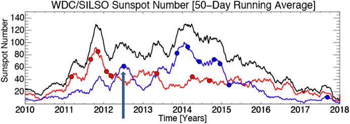
FIGURE 1. Sunspot cycle 24 as function of time; red denotes the cycle in the North, blue in South and the black curve denotes the total cycle. The near-miss Carrington type event occurred during July 12, marked by thick black arrow.

Simulating and predicting decadal-scale solar cycle features, namely the onset-timing, peak-amplitude and duration of a solar cycle, have received a lot of attention for more than half a century (see, e.g., Ohl, 1966). This is because the sinusoidal increase in solar activity produces similar increase in the energetic particle and radiation output from the Sun, which pervading through the interstellar and interplanetary space reaches the terrestrial system and can cause the beautiful aurorae as well as dreadful blackouts. However, a solar cycle does not really progress in a nice, smooth sinusoidal pattern. A close analysis of decadal solar activity curve, more precisely the sunspot cycle, reveals that the cycle actually progresses in the form of a quasiperiodic burst of enhanced solar activity followed by a relatively quiet phase. Figure 1 shows the solar cycle 24 progression based on monthly sunspot numbers; red is the sunspot cycle in the North, blue in the South and the black curve the total (N+S) cycle.

This short-term variability in solar cycle has long been recognized in the form of Rieger-type periodicity and quasi-biennial oscillation (QBO) by many authors starting from Rieger et al. (1984). There have been ample efforts to explore in detail the observational features of Rieger-periodicity and QBO, namely how they vary with solar cycle (see, e.g., Lean and Brueckner, 1989; Carbonell and Ballester 1990; Oliver et al., 1998; McIntosh et al., 2015; Gurgenashvili et al., 2016, Gurgenashvili et al., 2017), and also to simulate these periodicities by building theoretical models (Zaqarashvili et al., 2007, Zaqarashvili et al., 2010; Dikpati et al., 2017). Most importantly, it has recently been pointed out that these periodicities create similar periodicities in space weather (see, e.g., figure 3 of McIntosh et al., 2015), because major flares and CMEs occur during the enhanced bursts of solar activity, thus causing the “seasons” of space weather. We see in Figure 1 that a big X-class flare occurred during July 2012, which was like the Carrington event in strength, but the energetic particles and magnetic fields ejected from this flare barely missed hitting the Earth. The cycle 24, despite being the weakest in 100 years, caused such a dangerous flare, which occurred in a bursty phase of solar activity. In fact, the original Carrington even also occurred in a very weak solar cycle 10, but during an enhanced activity burst. Therefore, this short-term quasi-periodic variability in solar activity is as equally important to understand and predict as the forecast of the amplitude and timing of a decadal cycle, because it has been observed that major X- and M-class flares can occur primarily in the bursty phases, irrespective of the strength of the decadal cycle.

So, the question is: what causes this short-term variability, constituted of enhanced bursts and relatively quiet phases, in solar activity with an approximate periodicity of 6–18 months and in turn, similar space weather “seasons”? We note that the short-term or the “seasonal” variability in solar activity is connected with the physical mechanism of Rieger-type periodicities and QBO, which have been explored using MHD Rossby waves. While we are familiar with Earth’s Rossby waves, which play crucial roles in creating “jet stream” patterns that are used to forecast our daily weather, solar Rossby waves are no longer mere hypothesis; they have recently been observed using coronal brightpoints movements (McIntosh et al., 2017), coronal holes migration (Krista et al., 2018) and helioseismic measurements (Loptien et al., 2018; Hanasoge and Mandal, 2019). But a major difference between solar and planetary Rossby waves is that the Sun has strong magnetic fields, and hence solar Rossby waves are magnetically modified (see, e.g., Dikpati and McIntosh 2020; Zaqarashvili et al., 2021).

It has recently been demonstrated, using an MHD shallow-water model of plasma-fluid at/near the base of the convection zone in the tachocline, that the quasiperiodic enhanced bursts in solar activity can be caused through nonlinear, oscillatory exchange of energies among MHD Rossby waves, sunspot-producing magnetic fields and differential rotation (Dikpati et al., 2017; Dikpati et al., 2018a; Dikpati et al., 2018b). This nonlinear oscillation is called Tachocline Nonlinear Oscillations (or TNOs), which resemble the nonlinear Orr mechanism, their hydrodynamic counterparts in fluid mechanics. Studying such nonlinear interactions among Rossby waves, differential rotation and magnetic fields in the tachocline, for a wide range of parameters in the model, namely the differential rotation amplitude, the “effective gravity” of the plasma-fluid shell, the strength and latitude-location of the magnetic fields, these authors found (see, e.g., figure 4 in Dikpati et al., 2017) that the TNO periods fall within the range of 3–19 months, which is similar to the observed 6–18 months periods of “seasonal” variability in solar activity (see Figure 1 in Introduction section, and also see McIntosh et al., 2015 for details). However, all those simulations used banded toroidal fields of 10-degree latitudinal width for all cases.

While narrow bands of 10-degree latitudinal width are reasonable choice, since the surface observations of active regions’ diameter may indicate so (Zwaan, 1992), the shape and profile of these fields are not directly known at the tachocline level. In general the dynamo-generated spot-producing toroidal magnetic fields are most likely broad at/near the base of the convection zone (see, e.g., Dikpati and Charbonneau, 1999), but concentrated wreaths have also been found in the 3D convective dynamo simulations (Nelson et al., 2013). Furthermore, recent analysis indicates that the magnetic toroids, derived from surface magnetograms, can have latitudinal width broader as well as narrower than 10-degree at certain cycle phases (see, Dikpati et al., 2021, for details). Therefore, the first question that arises here is: would the TNO periods still fall within the observed range of periods for short-term, seasonal/sub-seasonal variability in solar activity and QBO if the activity bursts occur from a broader or narrower than 10-degree magnetic band?

Another aspect of the MHD shallow-water model, which was not explored by Dikpati et al. (2017) is how would the TNOs change if the spherical plasma-fluid shell is thicker or thinner than the thickness considered. Since the model was originally applied to the tachocline, the thickness of the model was taken to be no more than four percent of the solar radius. Shallow-water models are quasi-3D models, in which the horizontal extent and motions are much larger than that in the radial direction (Pedlosky, 1987). Subadiabatic stratification in the tachocline helps this model-condition to be satisfied, and hence application of this model in the solar tachocline was successfully implemented. However, shallow-water models can be applied to thicker spherical shells as long as the shell is located in a subadiabatically stratified region. In fact, in recent 3D convection simulations, Kapyla et al. (2017) have found that the entire lower half of the convection zone could be subadiabatically stratified. This means that the shell-thickness can be considered larger than tachocline thickness, extending the shell up to the middle of the convection zone. This raises the second question: how would the TNOs change if the shallow-water model is considered to be as thick as 15% of solar radius, extending from the bottom of the tachocline to the middle of the convection zone?

The purpose of this paper is to address these two questions, by studying the TNO properties for broader than 10-degree wide magnetic fields, and also for a thicker plasma-fluid shell. We will be employing here the already built nonlinear MHD shallow-water model of Dikpati et al. (2018a) to find answers to these questions. What follows are the mathematical formulation including description of the model and simulation set-up, results and concluding remarks.

Mathematical Formulation

Description of Model

Our starting point for the simulations here is the nonlinear MHD shallow-water model of Dikpati et al. (2018a). Even though the MHD shallow-water models of solar tachocline have been explored by many authors, it may be helpful for the general solar audience to present here a brief description The so-called shallow-water model is a class of model for studying the dynamics of incompressible flow in a sufficiently thin layer so that the horizontal extent and motions are much larger than the vertical extent and motions. Essentially the shallow-water equations were formulated to study Euler equations for a compressible fluid in which the pressure is quadratic with density, but the density of the fluid is replaced by the fluid thickness (see, e.g., Gill 1982; Pedlosky, 1987). The pressure perturbations are hydrostatic, determined by the weight (and hence the height) of the fluid column. In a single-layer shallow-water model, this weight is determined by the deformation of top surface of the fluid layer. The bottom boundary is rigid. The horizontal velocities are independent of radius, whereas the vertical velocity is a linear function of depth. This means, while flowing horizontally the fluid can stretch or compress in the vertical direction, therefore deforming the top surface due to mass conservation. Hydrodynamic shallow-water models have been applied to study oceanic and atmospheric flow patterns. For low Rossby number $R_o$ (i.e., the ratio between the typical rotation velocity and the rotation velocity of the spherical fluid shell), the flow is nearly geostrophic, i.e., it is in approximate horizontal force balance between the Coriolis forces and pressure gradients. Dikpati and Gilman (2001) have discussed in detail the very basic formalisms of a hydrodynamic shallow water model applied to the solar tachocline.

Since the Sun has strong magnetic fields, the shallow-water models have to be magnetohydrodynamic, particularly when applied at/near the base of the convection zone. Following Gilman (2000), various MHD shallow-water models for the solar tachocline have been developed (see, e.g., Gilman and Dikpati, 2002; Dellar, 2003, Zaqarashvili et al., 2007, Klimachkov and Petrosian, 2017). We briefly discuss the basis of formulation of an MHD shallow-water system. The magnetic fields in such a system are confined to the layer even when the top surface in deforms; essentially the magnetic fields resemble their hydrodynamic counterparts, the velocity fields, i.e., the horizontal magnetic field components are independent of height, whereas the vertical component is a linear function of height. Very much like the mass-conservation is satisfied, the total magnetic flux is conserved in the spherical shell, so that magnetic monopoles do not exist. This leads to the modified divergence-free condition for the magnetic field, namely the horizontal divergence of the product of shell-thickness and the horizontal magnetic field is zero. In a non-dissipative shallow-water system of “ideal plasma-fluid,” the total (magnetic plus kinetic plus potential) energy is conserved, when integrated over the entire volume of the shell.

Equations

The full set of MHD shallow-water equations have been presented in inertial frame (equations 1–6 of Gilman and Dikpati 2002) and in rotating frame of reference which is rotating with core-rotation rate (equations 1–6 of Dikpati et al., 2018a). These equations have been made nondimensional by selecting the radius $\left(r_0\right)$ of the shell to be the unit length and the inverse of core-rotation $\left({\omega }_c^{-1}\right)$ to be the unit time. Nondimensionalization also leads to a dimensionless parameter, $G=gH/\left(r_0^2 {\omega }_c^2\right)$, which represents the reduced gravity of the shell. Here g is the actual gravity at $r_0$ and $H$ is the total thickness of the shell. $G$ is a measure of the subadiabaticity of the layer.

These equations are solved using a pseudo-spectral algorithm, in which the time-integration is performed using Adams-Bashforth scheme. The detailed solution technique, including the application of a small numerical viscosity has been discussed in Dikpati (2012).

Results

Changes in TNO Properties With Variation in Shell-Thickness

Two examples of thickness of the spherical plasma-fluid shell of the MHD shallow-water model have been schematically presented in Figure 2, overlaying semi-transparent purple shade on top of the helioseismically derived rotation contours. The left panel shows the thin tachocline in which the MHD shallow-water models were previously applied, and the right panel shows a much thicker spherical shell that can plausibly be a subadiabatic layer as per simulation results of Kapyla et al. (2017).

FIGURE 2

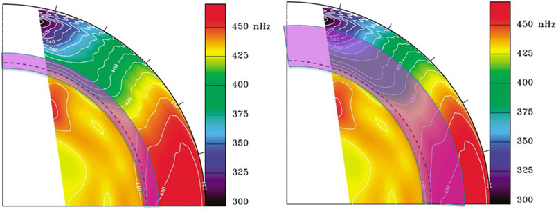
FIGURE 2. Schematically displayed, in semi-transparent purple-shades superimposed on the helioseismicly-derived solar internal rotation profiles (figure 3 of Thompson et al., 2003), two extreme cases of plausible thickness of the spherical shell in which shallow-water models can be applied: (left) very thin tachocline plasma-fluid shell and (right) much thicker shell extending up to the middle of the convection zone.

Since it is not clearly known whether the dynamo-generated magnetic fields can be equally strong in the entire thicker layer as in the thin tachocline, we compute TNOs using hydrodynamic shallow-water model. We keep all other parameters, namely we set the amplitude of the pole-to-equator latitudinal differential rotation to be 21%, with 12% amplitude in the μ² term and 9% in the μ⁴ term. We consider two different effective gravity value, namely G = 0.5 and G = 10. The TNO periods as function of shell-thickness have been plotted in Figure 3.

FIGURE 3

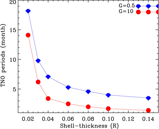
FIGURE 3. Simulated TNO periods as function of thickness of spherical shell of plasma-fluid. R denotes the solar radius.

We find that the TNO periods decrease with the increase in the thickness. This is understandable, because the thicker is the fluid-shell the heavier is the fluid-mass contained in it. Therefore, the available energy gets used up quickly, and the back-and-forth nonlinear exchange among energies takes place faster, resulting into smaller TNO periods.

We note that G = 0.5 case produces TNO periods much closer to observations of solar “seasons” than G = 10 case. This lower G case also fits better with Kapyla et al. (2017) results, which indicate slightly subadiabatic stratification in the bottom half of the convection zone, but rule out strongly the subadiabatic stratification.

Furthermore, the observed periods in the short-term variability in solar activity would suggest the thickness of the layer where the TNOs are originated. If we deduce various bins, in which the distribution of observed periods within the 6–18 months range would fall, it would be possible to derive what fraction of observed periods fall in a particular bin that would correspond to the TNO periods generated in a layer of a specific thickness. Then an average thickness of the shallow-water model can be favored, which may be significantly less than 10% of the solar radius, but this thickness may be having some time dependence.

Changes in TNO Properties With Variation in Latitudinal Width of Toroidal Band

Simulations of TNO for narrow toroidal magnetic bands of latitudinal widths of 10-degree were studied in detail by Dikpati et al. (2017, 2018a, 2018b). Very recently nonlinear magnetohydrodynamics of a slightly wider band of 14-degree latitudinal width have been studied in the context of understanding the features of Halloween storm of 2003 (see, e.g., figures 12–14 of Dikpati et al., 2021). We focus here in the magnetohydrodynamics of a much broader magnetic band of latitudinal widths of 30-degree, for example.

Using the expression (22) of Dikpati and Gilman (1999), namely, we set up the simulation for a broad band with 30-degree latitudinal width. We place a pair of oppositely-directed bands at 20-degree latitudes in the North and South hemispheres, and set the latitudinal widths $\left(\delta \vartheta \right)$, (i.e., the full-width at half maximum) of the band by using the expression $\delta \vartheta =2/\sqrt{{\beta }^{\prime }}$, in which ${\beta }^{\prime }=\beta \left(1-d_{sl}^2\right)$, $d_{sl}$ is the sine (latitude) of the band-center. As discussed in detail in Dikpati and Gilman (1999), $\left(1-d_{sl}^2\right)$ term takes care of the change in latitudinal width due the curvature of spherical geometry as the band location in latitude changes. Therefore, for our selected latitude of 20-degree in both North and South hemispheres, $\beta ={\beta }^{\prime }/\left(1-d_{sl}^2\right)=14.6$, with $d_{sl}=0.342$, will produce a 30-degree latitudinal width at 20-degree latitude. Furthermore, we select a pole-to-equator latitudinal differential rotation of 24% with equal contribution from the second $\left(s_2\right)$ and fourth order $\left(s_4\right)$ terms in the expression of differential rotation, given by $\omega =s_0-s_2{\mathit{\mu }}^2-s_4{\mathit{\mu }}^4-{\omega }_c$, μ represents the sine latitude, $\sin \left(\vartheta \right)$, ${\omega }_c$ the core-rotation rate, or equivalently the rotation rate at 32-degree latitude. The value of $s_0$ term thus makes the $\omega$ to be zero at 32-degree latitude for selected $s_2$ and $s_4$ terms. We present the nonlinear evolution of this pair of Gaussian bands for the peak field strength of 15 kGauss. Note that, unlike a broad $\sin \left(\vartheta \right)$ profile, just an amplitude of 0.15 will not make the peak field strength to be 15 kGauss in the case of a Gaussian band. A necessary prefactor is amplified to obtain the peak field strength of 15 kGauss.

Four panels in Figure 4 show the nonlinear evolution of the broad magnetic band, the mathematical prescription of which is described above. We selected nonuniform time intervals to display certain specific characteristics of the magnetic bands after 1, 4, 6 and 7 months respectively in the panels (a), (b), (c) and (d). To deduce the characteristics in these evolutionary patterns, namely when moderate and enhanced bursts of activity would occur, and when it would give rise to a relatively quiet period in solar activity, we first recall that the magnetic flux would buoyantly or convectively emerge to the surface if the flux-concentration occur at certain latitude-longitude locations of the spot-producing toroidal band at the tachocline, and/or if certain portions of the magnetic bands coincide with the bulging of the tachocline top-surface (see figure 1 of Dikpati et al., 2017). With these considerations, the evolution of latitude-longitude locations of flux-emergence have been compared with emerged active regions from observations for several Carrington rotations in figure 12 of Dikpati and McIntosh (2020). Therefore, we can understand our simulation results for a broad magnetic band using similar physical arguments, which we present below in a compact way.

FIGURE 4

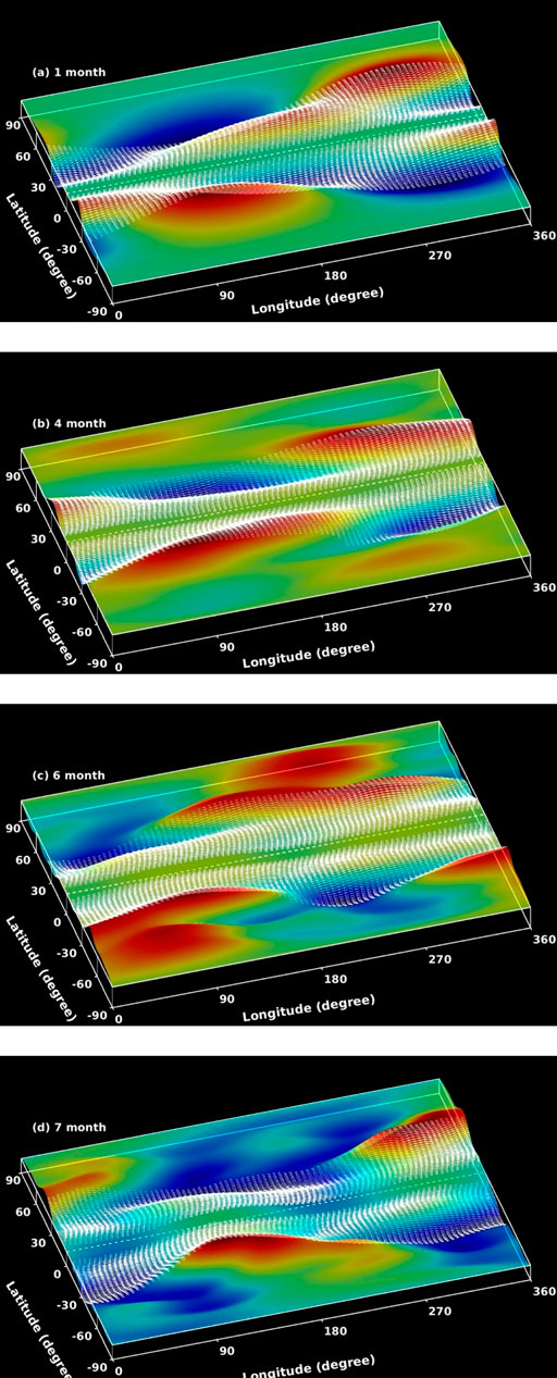
FIGURE 4. Broad magnetic band of 30-degree width in white arrows on tachocline top surface, which is presented in rainbow colormap. Red/orange represents bulges and deep-blue/blue the depression in plasma fluid. Panels (A–D) show the nonlinear evolution of the magnetic band due to the interaction of Rossby waves, which work on the mean differential rotation and spot-producing toroidal fields as perturbation. The times for these four snapshots are selected nonuniformly, to capture the important dynamics, respectively at 1,4, 6 and 7 months.

Scheme 1 for enhanced bursts of activity: In the MHD shallow-water modeling framework, biggest possibility of enhanced flux-emergence occurs (i) when the flux of the spot-producing magnetic band at a certain latitude-longitude location in the tachocline at/near the base of the convection zone has been concentrated enough compared to its surroundings, as well as (ii) when that portion of the band coincides with the bulging in the top-surface of the tachocline.

Scheme 2 for moderate bursts of activity: Again, in our modeling framework, moderate possibility of flux-emergence occurs from certain locations at which the flux is concentrated, but not in the depression. In this case, the buoyancy of the concentrated flux would help initiate the emergence. Another framework could lead to some flux emergences, namely from those locations at which the flux may not be concentrated enough, but coincides with bulgings. In this case, those portions of the band would enter the adiabatically stratified convection zone, and the despite containing weaker flux, these portions of the spot-producing bands could make their emergence to the surface by being convectively driven. So in this scheme, satisfying either one of the two conditions (i) and (ii) given in Scheme 1, can lead to moderate flux-emergences.

Scheme 3 for insignificant or no activity bursts: A relatively quiet period for solar activity can be expected, according to our modeling framework, when the portions of the band with much concentrated flux are in the depressed fluid, and hence in a deeper, strongly subadiabatic regions of the tachocline, or when the bulging portions are containing only very weak magnetic flux in a rarified portion of the band. During the nonlinear evolution of the spot-producing magnetic band, this scheme 3 is prevalent, hence preventing significant flux-emergence and resulting into a relatively quiet period of solar activity.

With the help of the aforementioned schemes 1–3, we can explain the four panels of Figure 4. In all panels, the white arrows denote the wide magnetic bands, oppositely directed in the North and South hemispheres, and the rainbow color-map denotes the tachocline top-surface bulgings (red) and depressions (blue). The neutral thickness (i.e., no bulging or no depression) regions are yellowish green. Since the shallow-water models are in hydrostatic force-balance, the bulging or red regions have the higher and the depression or blue regions have the lower pressures than the surrounding regions in the local neighborhood. In panel (a), we see flux concentrations (i.e., dense white arrows) at certain longitudes, such as around 0-degree and 360-degree in both hemispheres, at latitudes closer to the equator. While these flux concentrations do not coincide with bulgings, they are also not in the deep depression. Instead, they are in the neutral thickness. On the other hand, there is flux-spreading in certain bulging regions. These frameworks would satisfy the scheme 2, resulting into moderate flux emergence either from the strong flux-concentrations in the neutral thickness or from the weak-flux in the bulgings. To compare this framework with the phase of a bursty season, we refer to the Figure 1, for example, the relative increase in the solar activity during July-August of 2011.

After three more months, we see in panel (b) that, around the longitudes of zero and 360° degrees in the North and around 90–120° degrees in the South, the strong concentrations of magnetic flux (dense white arrows) coincide with the bulgings (red). There are also other longitude locations where sufficient flux-concentrations occur in the neutrally thick regions, and band-spreading occurs in the deep depression (blue) regions. Therefore, during this evolutionary stage of the band, the scheme 1 is most optimally satisfied. This could lead to the biggest possibility of the enhanced flux emergences. This evolutionary pattern can be compared with the epoch of September-October of 2011 in Figure 1, namely the peak of the season of solar activity.

Panel (c) shows the evolution of the magnetic band after two more months from that in panel (b). The model-output again corresponds to the scheme 2 in this case, like that in panel (a), i.e., the concentrated flux is neither in bulging, nor in the depression, but in the neutrally thick regions. Therefore, there is a possibility of moderate flux emergences from flux-concentrations, which would be buoyant compared to their local surroundings.

Also, from some weak flux in the bulging, which can already enter the convection zone with those bulging regions, being partially frozen in the plasma-fluid. This situation can be compared with the near-end of the enhanced bursty season, i.e., December 2011–January 2012 epoch in Figure 1.

During further evolution, we see in panel (d) that the flux-concentrations coincide with the depressed fluid regions, which fall in the strongly subadiabatic parts of the layer. This makes the buoyant emergence harder. There still could be some flux emergences from the bulging, if the bulging regions contain some flux. This evolutionary pattern would correspond to a relatively quiet period, as seen in Figure 1 during March-April of 2012.

The dynamical evolution of the magnetic bands in this case is governed by the interactions of energetically active retrograde Rossby waves, which are capable of extracting energies from the mean differential rotation and the toroidal magnetic fields. The TNO period in this case is about eight months, which is only very slightly higher than that found for narrower bands of 10-degree latitudinal widths with the same peak field strength. This is because the 30-degree wide band has more magnetic flux than a 10-degree band of the same peak field strength, and hence can provide the energy to be extracted by the Rossby waves for slightly longer time to drive the TNO.

As discussed in the previous paper by Dikpati et al. (2018a, see their figure 6), the TNO occurs due to the energy extraction by the tilted Rossby wave patterns through the Reynolds and Maxwell stresses, and also due to the phase difference between the HD and MHD Rossby wave patterns, which can play crucial roles in energy extraction by the mixed stress. In the HD case the eastward tilted patterns (i.e., the high-latitude part of the plasma pattern tilted more toward the east) can extract energy from the mean zonal flow through the action of Reynolds stress, whereas in the MHD case, the westward tilted patterns can extract energy through Maxwell stress. Obviously for westward tilted patterns the Reynolds stress tries to rebuild the zonal flow. The resulting TNO periods can thus be due to a complex interplay of energy exchanges among kinetic, magnetic and potential energies. The detailed energy extraction mechanisms, along with energy integrals, are given in the appendix of Dikpati et al. (2018a). In a forthcoming paper we will compute these integrals to quantitatively discuss the energy extractions for driving the TNOs.

We can qualitatively understand the physics by looking at the synoptic map of the simulated flow patterns for the broader band case we studied here. In Figure 5 we display the flow-vectors in black arrows, superimposed on the color-map of the tachocline top surface; red/orange denotes bulging and deep-blue/sky-blue the depressed fluid. The flow patterns for only the nonzero longitudinal modes are displayed for clarity. We present the snapshots for the same selected times as in Figure 4, namely the flow-vectors after one, four, six and seven months respectively in the panels (a–d). The flow-vectors are global compared to magnetic field vectors, which are confined approximately in the range of 5–35 degrees of latitude. Flow is primarily geostrophic, i.e., clockwise in bulges and anticlockwise in depressions in the North hemisphere, except occasionally at certain locations. Furthermore, by comparing the four panels of Figure 4 with the corresponding four panels of Figure 5, we can see that the flow-vectors are channeled by the concentrated magnetic field regions.

FIGURE 5

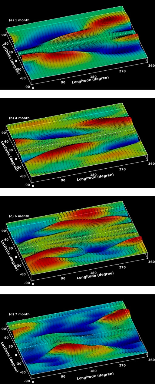
FIGURE 5. Flow vectors in black arrows for the broad magnetic band case superimposed on tachocline top surface, which is presented in rainbow colormap. Again as in Figure 4, red/orange represents bulges and deep-blue/blue the depression in plasma fluid. Panels (A–D) show the corresponding snapshots as in Figures 4A–D, nonuniformly selected respectively at 1,4, 6 and 7 months. But, unlike Figure 4, only the flow-component for nonzero longitudinal wavenumbers presented here, in order to understand the tilts in the hydrodynamic vorticity patterns in the Rossby waves.

Slow retrograde drifts are due to magnetically modified Rossby waves, but along with that we can see occasional appearance of fast gravity waves propagating in latitude, which establish the quick cross-equatorial communications. A careful look at these flow maps also reveals that the North-South asymmetry is larger during the first three panels, i.e., during the enhanced bursts of solar activity, than in panel (d).

We recall that we compared the snapshots in (a–c) of Figures 4, 5 with the enhanced solar activity during July–October of 2011. Whether the diminished North-South asymmetry is a more common feature of quiet solar season can be confirmed after many observational and model case studies.

Periodicity in Earth’s Radiation Belt in Van Allen Probe Data

The enhanced activity bursts can potentially have space weather impacts on Earth. As an example, a possible space weather impact on the Earth’s radiation belt is presented in Figure 6. The Earth’s radiation belts are inhabited by energetic ions and electrons. The relativistic electrons with energies >1 MeV are known as “killer electrons” because they can inflict damage to satellites and their onboard instruments at geosynchronous orbit (GEO) and low Earth orbit (LEO). It is well known that these radiation belt particles (electrons and ions) exhibit many periodicities at multi-time scales. For example, there is a decadal periodicity that corresponds to solar cycle, a 27-day periodicity due to the 27-days solar rotational period, a semiannual periodicity due to the Russel-Macpherron effect (Mchpherron et al., 2009), etc.

FIGURE 6

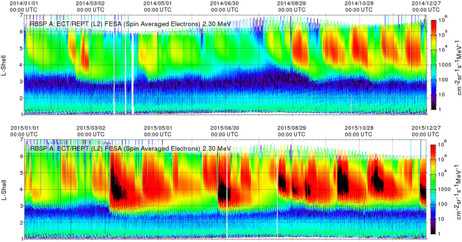
FIGURE 6. The averaged radiation belt 2.3 MeV electron fluxes from Van Allen Probe satellites in the period 2014–2015. The L-shell, which corresponds to distance from the Earth, is plotted on the Y-axis. The X-axis shows the time. The spectrogram shows that there are clusters of intense fluxes, which corresponds to enhanced activity bursts.

The solar wind has been known to be the primary driver of the radiation belt electron variabilities (e.g., Li et al., 2005; Reeves, 2007; Wing et al., 2016; Wing and Johnson, 2019). In particular, strong solar wind forcing such CMEs frequently lead to the productions of the relativistic electrons in the radiation belt (e.g., Blake et al., 1992; Baker et al., 2004; Reeves et al., 2013; Xiang et al., 2017; Baker et al., 2018; Baker et al., 2019; Pandya et al., 2019; Turner et al., 2019).

Van Allen Probe or Radiation Belt Storm Probe (RBSP) mission consisted of two identically instrumented spacecraft that were designed to observe the Earth’s radiation belt in 2012–2019 (Mauk et al., 2013). The Relativistic Electron-Proton Telescope (REPT) instrument on board of Van Allen Probes measured electrons with energy range 1.5 to ≥10 MeV (Baker et al., 2012). Figure 6 presents the spectrogram of the spin-averaged 2.3 MeV electron flux from RBSP REPT electron measurement for the period 2014–2015 obtained from The Johns Hopkins University Applied Physics Laboratory (JHU/APL) Van Allen Probe Science Gateway (https://rbspgway.jhuapl.edu/). The spectrogram shows that there are clusters of high fluxes.

The spectrogram shows that there are more active time periods (more periods of high fluxes) in 2015 than 2014. This trend may be attributed to the solar cycle as the sunspot number increases from 2014 to 2015. However, the solar cycle alone does not explain the clustering of the high fluxes, e.g., why there is a clustering of high fluxes in 2014 Aug–Dec and Feb. Russel-Mcpherron effect (i.e., the gain in southward component of IMF, which is more geoeffective near the spring and fall equinoxes due to certain tilt of Earth’s dipole) would place the high fluxes around the Mar 20th and Sep 23rd. So, this may explain some of the high fluxes in the Aug–Dec cluster, but not all of them (not in Nov and Dec). A careful look at the Figure 1 indicates correlation between high fluxes in the Earth’s radiation belt with the enhanced activity bursts during November-December of 2014. During this time the bursty seasons occurred in both hemispheres, along with several X- and M-class flares and CMEs. In a forthcoming paper, we will explore in more detail when this correlation is strongest and when there is a departure.

Summary and Conclusion

Previously it was found that the simulated TNO (Tachocline Nonlinear Oscillations) periods derived from an MHD shallow-water model fall within 3–19 months for a wide range of model-parameters, namely the differential rotation amplitudes, the effective gravity values, peak magnetic field strengths of a 10-degree band, and latitude-locations of the band. TNO periods are similar to that observed in the short-term variability of solar activity, and hence the TNO has been identified as one of the plausible causes of this quasi-annual seasons in solar activity and, in turn, space weather. Here we have studied how the TNO periods vary with band-width of the spot-producing toroidal fields and the thickness of the plasma-fluid layer, in which we apply the MHD shallow-water model. We find that the thicker is the layer the shorter is the TNO period, because the available energy for driving the TNO gets used up faster by the heavier fluid-mass contained in the thicker layer.

We have studied the nonlinear evolution of a wider band of 30-degree latitudinal width, which is much wider than a 10-degree band, but narrower than a fully broad band covering the latitude range from the equator to the pole in each hemisphere, because a fully broad toroidal field profile is known to open up into a clam-shell pattern (see, e.g., Cally, 2001; Cally et al., 2003). We find that the TNO period is much less sensitive with band-width; it is only very slightly larger for the wider band than the narrower with the same field strength. Wider band containing more magnetic flux than a narrow band can provide energy for a longer time for extraction to drive the TNO, hence the slight slow-down in TNO.

The electron flux in the Earth’s radiation belt shows a combination of various periodicities, one of which we find to be correlated with the quasi-periodic seasons in space weather with 6–18 months periodicity or the QBO and Rieger-type periodicity. Further analysis of much longer term data of electron fluxes is necessary to understand the physics of this correlation.

Also, it is not obvious what the observational signature of the North-South asymmetry at the Sun (as seen in the simulations presented in Figures 4, 5) would be at Earth. This would need to be investigated in light of the results in our study. There are certainly lots of north-south asymmetries in the Earth’s ionosphere and magnetosphere, but most of them can be attributed to the Earth’s dipole tilt or the dipole tilt angle with the Sun-Earth line.

Data Availability Statement

The raw data supporting the conclusions of this article will be made available by the authors, without undue reservation.

Author Contributions

MD contributes to the model and simulations of properties of short-term variability in solar activity, SM contributes to the observational analysis of quasi-periodic seasons in space weather and SW contributes to the impact of this variability in the Earth’s radiation belt electron fluxes.

Funding

This work is supported by the National Center for Atmospheric Research, which is a major facility sponsored by the National Science Foundation under cooperative agreement 1852977. We acknowledge support from several NASA grants; specifically, MD acknowledges LWS award 80NSSC20K0355 to NCAR, the subaward to NCAR from NASA’s DRIVE Center award 80NSSC20K0602 (originally awarded to Stanford), and NASA-HSR award 80NSSC18K1206 (originally awarded to NSO). SW acknowledges the support from NASA (Grant nos. NNX16AQ87G, 80NSSC20K0704, 80NSSC20K0355, 80NSSC19K0843, and 80NSSC20K0188).

Conflict of Interest

The authors declare that the research was conducted in the absence of any commercial or financial relationships that could be construed as a potential conflict of interest.

Acknowledgments

We thank Peter Gilman for reviewing this manuscript and for his helpful comments. We acknowledge the use of 200,000 core hours of high-performance computing in Cheyenne through NCAR Strategic Capability computing grant of 12 million core hours, with award No. NHAO0019 and also divisional computing grant P22104000 of HAO provided by NCAR’s Computational and Information Systems Laboratory.

References

Baker, D. N., Erickson, P. J., Fennell, J. F., Foster, J. C., Jaynes, A. N., and Verronen, P. T. (2018). Space Weather Effects in the Earth's Radiation Belts. Space Sci. Rev. 214, 17. doi:10.1007/s11214-017-0452-7

CrossRef Full Text | Google Scholar

Baker, D. N., Hoxie, V., Zhao, H., Jaynes, A. N., Kanekal, S., Li, X., et al. (2019). Multiyear Measurements of Radiation Belt Electrons: Acceleration, Transport, and Loss. J. Geophys. Res. Space Phys. 124, 2588–2602. doi:10.1029/2018JA026259

PubMed Abstract | CrossRef Full Text | Google Scholar

Baker, D. N., Kanekal, S. G., Hoxie, V. C., Batiste, S., Bolton, M., Li, X., et al. (2012). The Relativistic Electron-Proton Telescope (REPT) Instrument on Board the Radiation Belt Storm Probes (RBSP) Spacecraft: Characterization of Earth's Radiation Belt High-Energy Particle Populations. Space Sci. Rev. 179, 337–381. doi:10.1007/s11214-012-9950-9

CrossRef Full Text | Google Scholar

Baker, D. N., Kanekal, S. G., Li, X., Monk, S. P., Goldstein, J., and Burch, J. L. (2004). An extreme distortion of the Van Allen belt arising from the 'Hallowe'en' solar storm in 2003. Nature 432, 878–881. doi:10.1038/nature03116

PubMed Abstract | CrossRef Full Text | Google Scholar

Blake, J. B., Gussenhoven, M. S., Mullen, E. G., and Fillius, R. W. (1992). Identification of an Unexpected Space Radiation Hazard. IEEE Trans. Nucl. Sci. 39 (6), 1761–1764. doi:10.1109/23.211364

CrossRef Full Text | Google Scholar

Cally, P. S., Dikpati, M., and Gilman, P. A. (2003). Clamshell and Tipping Instabilities in a Two‐dimensional Magnetohydrodynamic Tachocline. ApJ 582 (2), 1190–1205. doi:10.1086/344746

CrossRef Full Text | Google Scholar

Cally, P. S. (2001). Nonlinear Evolution of 2D Tachocline Instabilities. Solar Phys. 199 (2), 231–249. doi:10.1023/a:1010390814663

CrossRef Full Text | Google Scholar

Carbonell, M., and Ballester, J. L. (1990). A Short-Term Periodicity Near 155 Day in Sunspot Areas. Astron. Astrophys. 238, 377–381.

Google Scholar

Dellar, P. J. (2003). Dispersive Shallow Water Magnetohydrodynamics. Phys. Plasmas 10, 581–590. doi:10.1063/1.1537690

CrossRef Full Text | Google Scholar

Dikpati, M., Belucz, B., Gilman, P. A., and McIntosh, S. W. (2018b). Phase Speed of Magnetized Rossby Waves that Cause Solar Seasons. ApJ 862 (2), 159. doi:10.3847/1538-4357/aacefa

CrossRef Full Text | Google Scholar

Dikpati, M., Cally, P. S., McIntosh, S. W., and Heifetz, E. (2017). The Origin of the “Seasons” in Space Weather. Scientific Rep. 7, 14750. doi:10.1038/s41598-017-14957-x

PubMed Abstract | CrossRef Full Text | Google Scholar

Dikpati, M., and Charbonneau, P. (1999). A Babcock‐Leighton Flux Transport Dynamo with Solar‐like Differential Rotation. ApJ 518, 508–520. doi:10.1086/307269

CrossRef Full Text | Google Scholar

Dikpati, M., and Gilman, P. A. (2001). Analysis of Hydrodynamic Stability of Solar Tachocline Latitudinal Differential Rotation Using a Shallow‐Water Model. ApJ 551 (1), 536–564. doi:10.1086/320080

CrossRef Full Text | Google Scholar

Dikpati, M., and Gilman, P. A. (1999). Joint Instability of Latitudinal Differential Rotation and Concentrated Toroidal Fields below the Solar Convection Zone. ApJ 512 (1), 417–441. doi:10.1086/306748

CrossRef Full Text | Google Scholar

Dikpati, M., McIntosh, S. W., Bothun, G., Cally, P. S., Ghosh, S. S., Gilman, P. A., et al. (2018a). Role of Interaction between Magnetic Rossby Waves and Tachocline Differential Rotation in Producing Solar Seasons. ApJ 853 (2), 144. doi:10.3847/1538-4357/aaa70d

CrossRef Full Text | Google Scholar

Dikpati, M., McIntosh, S. W., Chatterjee, S., Norton, A. A., Ambroz, P., Gilman, P. A., et al. (2021). Deciphering T He Deep Origin of Active Regions via Analysis of Magnetograms. Astrophys. J. 910, 24. doi:10.3847/1538-4357/abe043

CrossRef Full Text | Google Scholar

Dikpati, M., and McIntosh, S. W. (2020). Space Weather Challenge and Forecasting Implications of Rossby Waves. Space Weather 18, e2018SW002109. doi:10.1029/2018SW002109

CrossRef Full Text | Google Scholar

Dikpati, M. (2012). Nonlinear Evolution of Global Hydrodynamic Shallow-Water Instability in the Solar Tachocline. ApJ 745 (2), 128. doi:10.1088/0004-637x/745/2/128,

CrossRef Full Text | Google Scholar

Gill, A. E. (1982). “Atmosphere-Ocean Dynamics,” in International Geophysics Series (Academic Press), 30, 662.

Google Scholar

Gilman, P. A., and Dikpati, M. (2002). Analysis of Instability of Latitudinal Differential Rotation and Toroidal Field in the Solar Tachocline Using a Magnetohydrodynamic Shallow‐Water Model. I. Instability for Broad Toroidal Field Profiles. ApJ 576 (2), 1031–1047. doi:10.1086/341799

CrossRef Full Text | Google Scholar

Gilman, P. A. (2000). Magnetohydrodynamic “Shallow Water” Equations for the Solar Tachocline. Astrophys. J. Lett. 544 (1), L79–L82. doi:10.1086/317291

CrossRef Full Text | Google Scholar

Gurgenashvili, E., Zaqarashvili, T. V., Kukhianidze, V., Oliver, R., Ballester, J. L., Dikpati, M., et al. (2017). North–South Asymmetry in Rieger-type Periodicity during Solar Cycles 19–23. Astrophys. J. 845 (137), 11. doi:10.3847/1538-4357/aa830a

CrossRef Full Text | Google Scholar

Gurgenashvili, E., Zaqarashvili, T. V., Kukhianidze, V., Oliver, R., Ballester, J. L., Ramishvili, G., et al. (2016). Rieger-type Periodicity during Solar Cycles 14-24: Estimation of Dynamo Magnetic Field Strength in the Solar Interior. Astrophys. J. 826 (55), 10. doi:10.3847/0004-637x/826/1/55

CrossRef Full Text | Google Scholar

Hanasoge, S., and Mandal, K. (2019). Detection of Rossby Waves in the Sun Using Normal-Mode Coupling. Astrophys. J. Lett. 871 (L32), 5. doi:10.3847/2041-8213/aaff60

CrossRef Full Text | Google Scholar

Kapyla, P. J., Rheinhardt, M., Brandenburg, A., Arlt, R., Kapyla, M. J., Lagg, A., et al. (2017). Extended Subadiabatic Layer in Simulations of Overshooting Convection. Astrophys. J. 845 (L23), 6. doi:10.3847/2041-8213/aa83ab

CrossRef Full Text | Google Scholar

Klimachkov, D. A., and Petrosyan, A. S. (2017). Rossby Waves in the Magnetic Fluid Dynamics of a Rotating Plasma in the Shallow-Water Approximation. J. Exp. Theor. Phys. 125 (4), 597–612. doi:10.1134/s1063776117090059

CrossRef Full Text | Google Scholar

Krista, L. D., McIntosh, S. W., and Leamon, R. J. (2018). The Longitudinal Evolution of Equatorial Coronal Holes. Aj 155 (4), 153. doi:10.3847/1538-3881/aaaebf

CrossRef Full Text | Google Scholar

Lean, J. L., and Brueckner, G. E. (1989). Intermediate-term Solar Periodicities - 100-500 Days. ApJ 337, 568–578. doi:10.1086/167124

CrossRef Full Text | Google Scholar

Li, X., Baker, D. N., Temerin, M., Reeves, G., Friedel, R., and Shen, C. (2005). Energetic Electrons, 50 keV to 6 MeV, at Geosynchronous Orbit: Their Responses to Solar Wind Variations. Space Weather 3, a–n. doi:10.1029/2004SW000105

CrossRef Full Text | Google Scholar

Löptien, B., Gizon, L., Birch, A. C., Schou, J., Proxauf, B., Duvall, T. L., et al. (2018). Global-scale Equatorial Rossby Waves as an Essential Component of Solar Internal Dynamics. Nat. Astron. 2 (7), 568–573. doi:10.1038/s41550-018-0460-x

CrossRef Full Text | Google Scholar

Mauk, B. H., Fox, N. J., Kanekal, S. G., Kessel, R. L., Sibeck, D. G., and Ukhorskiy, A. (2013). Science Objectives and Rationale for the Radiation Belt Storm Probes Mission. Space Sci. Rev. 179 (1-4), 3–27. doi:10.1007/s11214-012-9908-y

CrossRef Full Text | Google Scholar

McIntosh, S. W., Cramer, W. J., Pichardo Marcano, M., and Leamon, R. J. (2017). The Detection of Rossby-like Waves on the Sun. Nat. Astron 1 (4), 0086. doi:10.1038/s41550-017-0086

CrossRef Full Text | Google Scholar

McIntosh, S. W., Leamon, R. J., Krista, L. D., Title, A. M., Hudson, H. S., Riley, P., et al. (2015). The Solar Magnetic Activity Band Interaction and Instabilities that Shape Quasi-Periodic Variability. Nat. Commun. 6 (1), 6491. doi:10.1038/ncomms7491

PubMed Abstract | CrossRef Full Text | Google Scholar

McPherron, R. L., Baker, D. N., and Crooker, N. U. (2009). Role of the Russel-McPherron effect in the acceleration of the relativistic electrons. J. Atmosph. Solar-Terrestr. Phys. 71 (10–11), 1032–1044. doi:10.1016/j.jastp.2008.11.002

Nelson, N. J., Brown, B. P., Brun, A. S., Miesch, M. S., and Toomre, J. (2013). Magnetic Wreaths and Cycles in Convective Dynamos. ApJ 762, 73. doi:10.1088/0004-637x/762/2/73

CrossRef Full Text | Google Scholar

Ohl, A. I. (1966). Wolf's number prediction for the maximum of the cycle 20. Solnice Dani 12, 84.

Oliver, R., Ballester, J. L., and Baudin, F. (1998). Emergence of Magnetic Flux on the Sun as the Cause of a 158-day Periodicity in Sunspot Areas. Nature 394, 552–553. doi:10.1038/29012

CrossRef Full Text | Google Scholar

Pandya, M., Bhaskara, V., Ebihara, Y., Kanekal, S. G., and Baker, D. N. (2019). Variation of Radiation Belt Electron Flux during CME‐ and CIR‐Driven Geomagnetic Storms: Van Allen Probes Observations. J. Geophys. Res. Space Phys. 124, 6524–6540. doi:10.1029/2019JA026771

CrossRef Full Text | Google Scholar

Pedlosky, J. (1987). Geophysical Fluid Dynamics. New York: Springer-Verlag, 710.

Reeves, G. D. (2007). Radiation Belt Storm Probes: A New Mission for Space Weather Forecasting. Space Weather 5, a–n. doi:10.1029/2007SW000341

CrossRef Full Text | Google Scholar

Reeves, G. D., Spence, H. E., Henderson, M. G., Morley, S. K., Friedel, R. H. W., Funsten, H. O., et al. (2013). Electron Acceleration in the Heart of the Van Allen Radiation Belts. Science 341 (6149), 991–994. doi:10.1126/science.1237743

PubMed Abstract | CrossRef Full Text | Google Scholar

Rieger, E., Share, G. H., Forrest, D. J., Kanbach, G., Reppin, C., and Chupp, E. L. (1984). A 154-day Periodicity in the Occurrence of Hard Solar Flares?. Nature 312, 623–625. doi:10.1038/312623a0

CrossRef Full Text | Google Scholar

Thompson, M. J., Christensen-Dalsgaard, J., Miesch, M. S., and Toomre, J. (2003). The Internal Rotation of the Sun. Annu. Rev. Astron. Astrophys. 41, 599–643. doi:10.1146/annurev.astro.41.011802.094848

CrossRef Full Text | Google Scholar

Turner, D. L., Kilpua, E. K. J., Claudepierre, S. G., O'Brien, T. P., Fennell, J. F., Blake, J. B., et al. (2019). The Response of Earth's Electron Radiation Belts to Geomagnetic Storms: Statistics from the Van Allen Probes Era Including Effects from Different Storm Drivers. J. Geophys. Res. Space Phys. 124, 1013–1034. doi:10.1029/2018JA026066

CrossRef Full Text | Google Scholar

Wing, S., and Johnson, J. R. (2019). Applications of Information Theory in Solar and Space Physics. Entropy 21 (2), 140. doi:10.3390/e21020140

PubMed Abstract | CrossRef Full Text | Google Scholar

Wing, S., Johnson, J. R., Camporeale, E., and Reeves, G. D. (2016). Information Theoretical Approach to Discovering Solar Wind Drivers of the Outer Radiation Belt. J. Geophys. Res. Space Phys. 121, 9378–9399. doi:10.1002/2016JA022711

CrossRef Full Text | Google Scholar

Xiang, Z., Tu, W., Li, X., Ni, B., Morley, S. K., and Baker, D. N. (2017). Understanding the Mechanisms of Radiation Belt Dropouts Observed by Van Allen Probes. J. Geophys. Res. Space Phys. 122, 9858–9879. doi:10.1002/2017JA024487

CrossRef Full Text | Google Scholar

Zaqarashvili, T. V., Carbonell, M., Oliver, R., and Ballester, J. L. (2010). Quasi-biennial Oscillations in the Solar Tachocline Caused by Magnetic Rossby Wave Instabilities. ApJ 724 (1), L95–L98. doi:10.1088/2041-8205/724/1/l95

CrossRef Full Text | Google Scholar

Zaqarashvili, T. V., Albekioni, M., Ballester, J. L., Bekki, Y., Biancofiore, L., Birch, A. C., et al. (2021). Rossby Waves in Astrophysics. Space Sci. Rev. 217 (1), 15. doi:10.1007/s11214-021-00790-2

CrossRef Full Text | Google Scholar

Zaqarashvili, T. V., Oliver, R., Ballester, J. L., and Shergelashvili, B. M. (2007). Rossby Waves in “Shallow Water” Magnetohydrodynamics. A&A 470 (3), 815–820. doi:10.1051/0004-6361:20077382

CrossRef Full Text | Google Scholar

Zwaan, C. (1992). “The Evolution of Sunspots,” in Sunspots: Theory and Observations. NATO ASI Series (Series C: Mathematical and Physical Sciences). Editors J. H. Thomas, and N. O. Weiss (Dordrecht: Springer), 375, 75–100. doi:10.1007/978-94-011-2769-1_3

CrossRef Full Text | Google Scholar