Thermospheric Neutral Winds as the Cause of Drift Shell Distortion in Earth’s Inner Radiation Belt

1. Introduction

The Van Allen Probes (Mauk et al., 2013) have provided unprecedented amounts of high quality energetic (10–100 keV) electron flux measurements near the magnetic equator in the inner belt and slot region (Reeves et al., 2016) below an equatorial altitude of about 3 Earth Radii ($L<3$). These new measurements confirmed known dynamical features such as “zebra stripe” patterns in the spectrograms of energetic electrons (Imhof and Smith, 1965; Ukhorskiy et al., 2014) and energetic electron injections deep into the inner magnetosphere (Pfitzer and Winckler, 1968; Turner et al., 2015). Electron flux measurements in the 100–400 keV energy range from the Magnetic Electron Ion Spectrometer (MagEIS) instruments (Blake et al., 2013) also revealed a surprisingly persistent local time asymmetry of the equatorial electron intensity below $L=1.4$ during geomagnetically quiet times, with higher radiation belt electron intensities near dawn (Selesnick et al., 2016).

Radiation belt particles are magnetically trapped high energy particles whose motion exhibits three quasi-periodic types of motion occurring on three distinct timescales (e.g., Northrop and Teller, 1960). The slowest periodicity corresponds to a drift motion around the planet that is the combination of an energy-independent electric drift and a gradient-curvature magnetic drift proportional to the particle’s momentum. Radiation belt particles’ drift motion defines closed surfaces known as drift shells. At high enough energies (>100 keV), the role played by large-scale electric fields is usually omitted: Radiation belt particles’ momentum is expected to be conserved along a drift shell and the flux is expected to be constant at a fixed $L$ value in the absence of any significant source or loss mechanism (e.g. Roederer, 1967). The observed local time asymmetry of the equatorial electron intensity at fixed $L$ values below $L=1.4$ challenged the latter, suggesting a drift shell distortion by a quasi-static electric field.

Even during geomagnetically quiet times, large-scale electric fields of the inner magnetosphere are more complex than the simple superposition of 1) a corotation electric field due to the rigid corotation of a perfectly conducting ionosphere and 2) a convection electric field set up by the coupling between the solar wind and the magnetosphere (e.g. Wolf et al., 2006). Dynamo electric fields produced by tidal motion of upper atmospheric winds flowing across the Earth’s magnetic field lines—the ionospheric wind dynamo (Richmond, 1989)—are usually larger than subauroral convection electric fields below L ∼ 2 (e.g., Figure 1 in the review by Mozer (1973). Longitudinal, seasonal, and solar cycle variations of the mid- and low-latitude ionospheric electric fields have been reported, together with a large day-to-day variability present even during geomagnetically quiet times (e.g., Fejer, 1993; Chau et al., 2010; Pfaff et al., 2010).

The objective of this study is to re-examine the time interval analyzed by Selesnick et al. (2016) in order to determine the origin of the large-scale electric field causing the observed radiation belt distortion. Observational and modeling resources are introduced in Section 2 to describe the electric field properties associated with the drift shell distortion observed. In particular, we present a method to infer electric field properties directly from an analysis of asymmetries measured in differential directional fluxes. Experimental, numerical and analytical experiments provide consistent electric potential variation estimates, of the order of $6-8kV$ between the dawn and dusk sectors at the magnetic equator of $L=1.30$, i.e. at a magnetic latitude of $\sim 29°$ at the ionospheric field line footpoint (Section 3). The similarities between experimental data analysis and outputs from a quiet time run by the Rice Convection Model (RCM) Coupled Thermosphere-Ionosphere-Plasmasphere-electrodynamics (CTIPe) model suggests that the electric potential variation results mainly from the quiet time wind dynamo.

2. Materials and Methods

Leveraging Liouville’s theorem and adiabatic invariant theory, we conduct an analysis of energetic electron directional differential fluxes measured by the Van Allen Probes to infer electric field properties in the inner belt. The resulting electric field properties are compared with outputs from Van Allen Probes field measurements and from a physics-based coupled model, RCM-CTIPe.

2.1. Field and Particle Measurements Onboard the Van Allen Probes

The time interval of the study corresponds to the first 60 days of the year 2014. This time interval was also selected for the study by Selesnick et al. (2016) because 1) the two orbital legs are near dawn and dusk at $L=1.3$ and 2) it is geomagnetically quiet. Although some moderate (Echer et al., 2006) geomagnetic activity occurs towards the end of February, the time interval contains no significant inner belt injection. Additional details on the geomagnetic conditions associated with this time interval are provided in Section 4.

The Van Allen Probes (Fox and Burch, 2014) were twin spacecraft with similar highly elliptical orbits (perigee at $\sim 600km$, apogee at $\sim 5.8R_E$), an orbital period of about 9 h, and an inclination close to $10°$. Spacecraft apogees drifted slowly so that it took a bit less than 2 years for spacecraft apogees to scan all local time sectors (precession rate of about $210°$ per year). Successive inbound and outbound crossings of $L=1.3$ occurred fast, within 30 min. During the first 60 days of 2014, inbound crossings of $L=1.3$ are in the dusk-premidnight region (20–22 MLT) while outbound crossings are in the dawn sector (4-6 MLT) for both Van Allen probes. The geographic longitudes of the crossings depend on time (UT).

In this study, we rely primarily on the directional differential fluxes provided by the MagEIS instrument (processed to level 3). Electric field measurements are also analyzed to compare and contrast with proposed electric field models. Experimental electric field information comes from measurements by the Electric Field and Waves (EFW) instrument (Wygant et al., 2013) and by the Electric and Magnetic Field Instrument Suite and Integrated Science (EMFISIS) (Kletzing et al., 2013). Field and particle measurements immediately following spacecraft maneuvers are omitted.

2.1.1. Differential Fluxes for Equatorial Electrons

The analysis focuses on equatorial electron intensity in the 150–400 keV energy range. MagEIS data below 400 keV is normally well above background. We follow the approach developed by Selesnick et al. (2016) to determine fluxes of equatorially mirroring electrons. MagEIS pitch-angle resolved measurements are extrapolated when the spacecraft is close to the magnetic equator. Specifically, directional differential fluxes are extrapolated to determine the equatorial electron intensity, $j_o$, when the local field magnitude, $B$, is such that $B_o\le B<1.08B_o$, where $B_o$ is the equatorial magnetic field calculated according to the International Geomagnetic Reference Field to which Olson and Pfitzer, 1977 Quiet is superimposed (Olson and Pfitzer, 1977).

We define the magnetic shell parameter, $L$, following the definition provided by McIlwain (1961). For equatorial particles, the parameter $L$ is such that:

$L={\left(B_E/B_o\right)}^{1/3}(1)$

where $B_E=\mathrm{30,000}nT$ is the magnetic equatorial field at the surface of the Earth. This definition guarantees that constant $L$ values define curves of constant equatorial magnetic field amplitude, i.e., $\left(B_o=cst.\right)\iff \left(L=cst.\right)$, even in non-dipolar fields.

When experimental information is required at a fixed $L$ value, we interpolate as a function of $L$ using adjacent measurements within $\pm 0.025L$ when available. Linear interpolations of adjacent logarithmic flux measurements are also performed to estimate partial derivatives with respect to $L$ and kinetic energy, $T$ (with window sizes of $\pm 0.025L$ and $\pm 155keV$, respectively).

2.1.2. Electric Drift Measurements

Electric drift measurements are pre-processed following the approach developed over the years by Lejosne and Mozer (2016a, 2016b, 2019) and briefly described below. After a slight correction applied to the orientation of the magnetometer axes (Lejosne and Mozer, 2016a), the spin-averaged ($\sim 12s$) electric drift measurement is reformulated in a local orthonormal frame of reference (${\mathit{e}}_{\mathit{\rho }},{\mathit{e}}_{\mathit{b}},{\mathit{e}}_{\mathit{\phi }}$) set by the measured magnetic field direction: ${\mathit{e}}_{\mathit{b}}=-\mathit{B}/\Vert \mathit{B}\Vert$, ${\mathit{e}}_{\mathit{\phi }}=\left(\mathit{B}\times \mathit{r}\right)/\Vert \mathit{B}\times \mathit{r}\Vert$ and ${\mathit{e}}_{\mathit{\rho }}={\mathit{e}}_{\mathit{\phi }}\times \mathit{B}/\Vert \mathit{B}\Vert ,$ where $\mathit{B}$ is the magnetic field vector at the location r. ${\mathit{e}}_{\mathit{\rho }}$ and ${\mathit{e}}_{\mathit{\phi }}$ indicate the radial and azimuthal directions, respectively. The shorting factor is calibrated to a value very close to 1 (Lejosne and Mozer, 2019). Once corotation is subtracted, the electric drift measurement is projected to the magnetic equator assuming equipotential field lines. The magnetic field model is set to the International Geomagnetic Reference Field for the Earth’s internal field. The choice of the external magnetic field model is unimportant when mapping at L = 1.30. During data processing, the Kp-driven Tsyganenko (1989) magnetic field model was superimposed (Lejosne and Mozer, 2016b).

2.2. Numerical Model RCM-CTIPe

Electric potential and electric field values at $100km$ altitude are provided by the Rice Convection Model (RCM) Coupled Thermosphere-Ionosphere-Plasmasphere-electrodynamics (CTIPe) model. This self-consistently coupled model of the magnetosphere, ionosphere and thermosphere is composed of three physical models: 1) the Coupled Thermosphere-Ionosphere-Plasmasphere with self-consistent electrodynamics (CTIPe) model (Fuller-Rowell et al., 1996; Millward et al., 2001, 1996); 2) the Rice Convection Model—RCM (Toffoletto et al., 2003; Wolf, 1983); and 3) the global electrodynamic solver based on the National Center for Atmospheric Research Thermosphere-Ionosphere Electrodynamics General Circulation Model—NCAR-TIEGCM (Richmond and Maute, 2014). The model includes the electrodynamic coupling, interactions, and feedback between the inner magnetosphere and the thermosphere-ionosphere-magnetosphere system. A detailed description of the model coupling can be found in the article by Maruyama et al. (2011).

2.3. Theoretical Framework for the Inference of Electric Field Properties From Directional Differential Flux Analysis

The objective of this section is to show how to infer information on electric field properties from measured variations of differential fluxes of equatorially trapped particles. This theoretical framework is similar to the one developed by Lejosne and Mozer (2020) for the analysis of zebra stripe patterns. It is adapted below to the case of drift shell distortion by quasi-static electric fields.

Leveraging Liouville’s theorem and adiabatic invariant theory, the variation of equatorial electron fluxes measured at different local times along the same $B_o=cst$. curve is related to trapped particle kinetic energy variation (Section 2.3.1.). Section 2.3.2. details the relationship between trapped particle kinetic energy variation and electric potential variation. Section 2.3.3. provides the equation implemented hereafter and summarizes the assumptions underlying the overall approach.

2.3.1. Link Between Fluctuations in Directional Differential Fluxes of Equatorially Trapped Particles and Kinetic Energy Variations

According to Liouville’s theorem, the phase space density, $f=j_o/p^2$, is constant along the continuous trajectories of the system in phase space, i.e., along the dynamical path of particles, in the absence of any source or loss. Thus, any variation of the trapped population momentum, $dp/p$, is related to a variation of the directional differential flux, $d{j}_o/j_o$ along the drift shell:

$\frac{d{j}_o}{j_o}=2\frac{dp}{p}(2)$

This equation can also be rewritten in terms of kinetic energy, $T$, and kinetic energy variation, $dT$, since:

$\frac{dp}{p}=\frac{\gamma }{\gamma +1}\frac{dT}{T}(3)$

where $\gamma =(T+m{c}^2)/m{c}^2$ is the Lorentz factor and $m{c}^2=511keV$ is the rest mass energy for an electron. Assuming conservation of the first invariant, $p^2/2m{B}_o=cst.$, any variation of the momentum is related to a variation in the equatorial magnetic field along the drift shell:

$2\frac{dp}{p}=\frac{d{B}_o}{B_o}(4)$

Noting that $B_o=B_E/L^3$(Eq. 1), the combination of Eqs 3, 4 also relates trapped particle energization, $dT$, and radial motion, $dL$:

$\frac{dT}{T}=-\frac{3}{2}\left(1+{\gamma }^{-1}\right)\frac{dL}{L}(5)$

The variations discussed above occur along the same equatorial drift shell, i.e.:

$d{j}_o=j_o\left(T+dT,B_o+d{B}_o,{\phi }_2\right)-j_o\left(T,B_o,{\phi }_1\right)(6)$

where $(T,B_o,{\phi }_1)$ and $(T+dT,B_o+d{B}_o,{\phi }_2)$ are coordinates along the same equatorial drift shell. The phases ${\phi }_1$ and ${\phi }_2$ represent the magnetic local times of an $L$-crossing during consecutive inbound and outbound passes, respectively. In practice, the shape of the distorted drift shell is unknown, and what is measured is in fact the fluctuation in differential equatorial flux at fixed kinetic energy, $T$, and different magnetic local times along the same $B_o=cst$. curve. In other words, the fluctuation measured is:

$\delta j_o=j_o\left(T,B_o,{\phi }_2\right)-j_o\left(T,B_o,{\phi }_1\right)(7)$

Assuming small distortions of the field, the fluctuation measured, $\delta j_o$, is related to the fluctuation along the dynamical path of particles, $d{j}_o$, in the following way:

$\delta j_o=d{j}_o-dT\frac{\partial j_o}{\partial T}-d{B}_o\frac{\partial j_o}{\partial B_o}(8)$

Combining Eqs 3, 4 and 8, and noting that $dx/x=d\ln x$, we obtain the relationship between the variation of equatorial electron differential fluxes measured at different local times along the same $B_o=cst$. curve, $\delta j_o$, and trapped particle energy variation, $dT$:

$\frac{\delta j_o}{j_o}=\left(\frac{2\gamma }{\gamma +1}\left(1-\frac{\partial \ln j_o}{\partial \ln B_o}\right)-\frac{\partial \ln j_o}{\partial \ln T}\right)\frac{dT}{T}(9)$

2.3.2. Link Between Kinetic Energy Variation and Electric Potential Variation

The time rate of change of the average kinetic energy of a guiding center of charge $q$ is provided by the energy equation (Roederer and Zhang, 2014):

$\frac{dT}{dt}=\frac{M}{\gamma }\frac{\partial B}{\partial t}+\mathit{V}\cdot \left(q\mathit{E}+\mathit{F}\right)(10)$

where $\mathit{V}$ refers to the drift velocity of the guiding center and $\mathit{F}$ is an external non-electromagnetic force that is omitted hereafter. The electric field, $\mathit{E}$, is described here as the sum of a corotation electric field and a subauroral electrostatic field:

$E=-\left(\mathbf{\Omega }\mathrm{\times }\mathbf{r}\right)\mathrm{\times }\mathbf{B}-\nabla U(11)$

where Ω is the angular velocity vector of the Earth’s rotation, and $U$ is the electrostatic potential associated with the subauroral electrostatic field. Noting that $\partial B/\partial t=-\left(\mathit{\Omega }\times \mathit{r}\right)\cdot \nabla B$, it follows from the combination of Eqs 10, 11 in the case of energetic electrons ($q<0)$ that a variation in kinetic energy, $dT$, along the dynamical path of particles is related to a variation in electrostatic potential, $dU$:

$dT=e\left(1-\varsigma \left(T\right)\right)dU(12)$

where $e=\left|q\right|>0$ is the elementary charge and $\varsigma \left(T\right)$ corresponds to the ratio between electric and total (magnetic + electric) angular drift velocities

$\varsigma \left(T\right)\cong e\frac{2}{3}\left(\frac{\gamma }{\gamma +1}\right)\frac{\Omega B_E{R}_E^2}{TL}\ll 1(13)$

where $R_E=\mathrm{6,370}km$ is one Earth radius. Eq. 12 describes the conservation of the total energy of the guiding center along the drift shell (e.g., Whipple, 1978).

2.3.3. Summary of the Theoretical Framework

A change of variables from $B_o$ to $L$ (Eq. 1) and the combination of Eqs 9, 12 provides the relationship between a measured fluctuation in the equatorial electron intensity, $\delta j_o$, and an electrostatic potential variation, $dU$. Let us emphasize that the variations measured are between the magnetic local times of the inbound (${\phi }_1$) and outbound (${\phi }_2$) crossings of the same $B_o=cst$. curve:

$dU=\frac{T\left(1+\varsigma \left(T\right)\right)}{e}{\left(\frac{2\gamma }{\gamma +1}\left(1+\frac{1}{3}\frac{\partial \ln j_o}{\partial \ln L}\right)-\frac{\partial \ln j_o}{\partial \ln T}\right)}^{-1}\frac{\delta j_o}{j_o}(14)$

where $\delta j_o=j_o\left(T,B_o,{\phi }_2\right)-j_o\left(T,B_o,{\phi }_1\right)$, and the partial derivatives are computed outbound at $\left(T,B_o,{\phi }_2\right)$.

Theoretically, the electric potential variation, $dU$, on the left side of Eq. 14, is a quantity independent of the kinetic energy of the trapped population considered, $T$. Thus, the right side of Eq. 14 is expected to be independent of the variable $T$ as well.

The assumptions underlying this equation are that there is no significant source or loss mechanism on the time scale of the equatorially trapped population drift period, no external non-electromagnetic force, no parallel electric field, no other significant source of magnetic field time variation besides Earth’s rotation, and no significant time variation of the electric potential on the timescale of the electron drift period (this includes the timescale of spacecraft motion from the inbound to the outbound crossings of $L=1.3$, which is of the order of $30min$).

3. Results

Section 3.1. presents experimental information on the electric potential variation between dawn and dusk at $L=1.30$ (magnetic latitude of $\sim 29°$ at the corresponding ionospheric field line footpoint), leveraging field and particle measurements independently. Section 3.2. compares these results with estimates from analytical and numerical models. Section 3.3.Conclusion of the Experimental Analysis summarizes our findings.

3.1. Experimental Results

3.1.1. Experimental Information on the Electric Potential Variation Between Dawn and Dusk Based on Measured Equatorial Electron Intensity Asymmetry

Figure 1 is an introduction to the approach. During the first 60 days of 2014, the Van Allen Probes crossings of $L=1.30$ are in the dusk-premidnight region (20–22 MLT) during inbound, ${\phi }_1$, and in the dawn (4-6 MLT) sector during outbound, ${\phi }_2$ (Figure 1A). The equatorial intensity of 226 keV electrons at $L=1.30$ measured by Van Allen Probes A (RBA) is ∼40% higher at dawn (in red Figure 1B) than dusk (in blue Figure 1B). The corresponding equatorial intensity fluctuation at 226 keV and $L=1.30$, $\delta j_o/j_o$, is evaluated by subtracting the outbound electron intensity (the red line Figure 1B) from the inbound electron intensity (the blue line Figure 1B), and normalizing by the inbound value. This was done for 40 different consecutive sequences of near equatorial inbound/outbound crossings of $L=1.3$ during the 60 days considered (Figure 1C). The partial derivatives of $\ln j_o$ with respect to $\ln L$ and $\ln T$ were computed locally to provide a time series for the electric potential variation, $dU$, between the inbound and outbound local times of $L=1.30$ following Eq. 14 (Figure 1D).

FIGURE 1

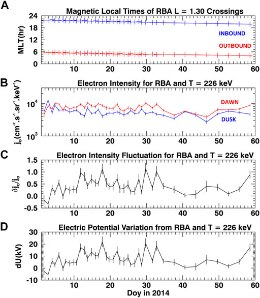
FIGURE 1. The variation of electric potential between the inbound and outbound locations of the same $L=1.30$ value is inferred directly from an analysis of asymmetries in measured energetic electron fluxes. (A) Magnetic local times of the Van Allen Probes A, RBA, during (blue) inbound and (red) outbound crossings of $L=1.30$; (B) Equatorial electron intensity at 226 keV during (blue) inbound and (red) outbound crossings of $L=1.30$, derived from measurements at 226 keV by the MagEIS instrument onboard Van Allen Probes A; (C) Corresponding fluctuations in directional differential fluxes of equatorially trapped 226 keV electrons; and (D) Corresponding electric potential variation at $L=1.30$ between dawn and dusk, the local times of the outbound and inbound crossings, respectively. The 1-sigma error bars are derived from statistical error in each measured $j$ value.

The time variation of the electric potential variation, $dU\left(t\right)$, is similar to the time variation of the intensity fluctuation, $\delta j_o/j_o\left(t\right)$, because the coefficient by which $\delta j_o/j_o$ is multiplied to obtain $dU$ (Eq. 14) does not vary significantly (<10%) during the time interval considered. Analysis of the 226 keV equatorial electron intensity measured by Van Allen Probes A during the first 60 days of 2014 suggests that the average electric potential variation between dawn and dusk is $7.6\pm 2.7kV$.

The approach is extended to both Van Allen Probes, and to all four MagEIS energy channels between 150 and 400 keV. The results are presented Figure 2. While the times series for the electric potential variations seem to depend on the measuring spacecraft (Figures 2A,B), the averages, and standard deviations of the electric potential variation, $dU$, appear independent of the energy channel (Figure 2C). That the statistical characteristics of the electric potential do not depend on MagEIS energy channel is consistent with theoretical expectations (Section 2.3.3.).

FIGURE 2

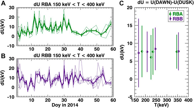
FIGURE 2. (A) Time series of electric potential variations according to four MagEIS channels comprised between 150 and 400 keV onboard the Van Allen Probes A (RBA). The time series inferred from each individual energy channel are represented by thin lines while the average over all four energy channels is represented by a thick solid green line. (B) Time series of electric potential variations according to four MagEIS channels comprised between 150 and 400 keV onboard the Van Allen Probes B (RBB). The time series for each energy channel are represented by thin lines while the average over all four energy channels is represented by a thick solid purple line. (C) Medians and standard deviations for the electric potential variation between dawn and dusk at L = 1.3 during the first 60 days of the year 2014 according to four MagEIS channels measuring differential direction fluxes for kinetic energies, $T$, comprised between 150 and 400 keV, onboard (green) Van Allen Probes A and (purple) Van Allen Probes B.

The analysis suggests that the average value for the electric potential variation between dawn and dusk is $dU=8\pm 4kV$ during the first 60 days of 2014. In terms of average electrostatic field, since $dU=-{\displaystyle \underset{{\phi }_1}{\overset{{\phi }_2}{\int }}\mathit{E}.\mathit{dl}}\cong -{\displaystyle \underset{{\phi }_1}{\overset{{\phi }_2}{\int }}{E}_{\phi }{r}_{o}d\phi }$, the electric potential variation corresponds to an average radial electric field between dusk (${\phi }_1$) and dawn (${\phi }_2$) of $\left[E_{\phi }\right]=-0.5\pm 0.2mV/m$ at the magnetic equator of $L=1.3$.

3.1.2. Experimental Information on the Electric Potential Between Dawn and Dusk Based on Electric Field Measurements

While Van Allen Probes only provide local electric field samples at $L=1.3$ at precisely dusk (${\phi }_1$) and dawn (${\phi }_2$) during the time interval considered, it is possible to obtain another estimate of the electric potential variation between dawn and dusk by considering Van Allen Probes electric field measurements over a longer time interval. Figure 3 provides experimental information on the characteristics of the DC electric field measured by the Van Allen Probes during the years 2013 and 2014 at $L=1.3\pm 0.05$ during geomagnetically quiet times ($Kp<3$). The local time averages and standard deviations are computed over running windows of 1 hour size and they are represented by a black line and a shaded area, respectively. Assuming that the electrostatic electric field ($-\nabla U$) is quasi-stationary, the 24 hr-MLT average of the electric field components should be zero. Experimentally, the 24 hr-MLT averages of the radial and azimuthal electric field components measured are $0.02mV/m$ and $0.20mV/m$, respectively. These small offsets could be due to small residual calibration errors (e.g. Lejosne and Mozer, 2019). They could also be due to the irregular seasonal and longitudinal samplings. These small offsets have been subtracted from the datasets before estimating the average electric field between dusk and dawn and the corresponding electric potential variation between dawn and dusk. In that context, the average azimuthal component of the electric field between dusk and dawn is $-0.4\pm 0.1mV/m$, and the corresponding variation of the electric potential is $7\pm 2kV$. These are comparable to the estimates provided by the particle data analysis (Section 3.1.1.).

FIGURE 3

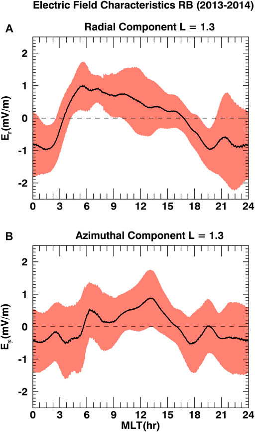
FIGURE 3. Characteristics of the (A) radial and (B) azimuthal components of the electric field measured by both Van Allen Probes and projected to the magnetic equator during crossings of $L=1.3$ in the years 2013 and 2014. The solid black lines are the 1hr-MLT running averages of the data points. The standard deviation computed over the same 1 hr-MLT running window is represented by the shaded area. The 24 hr-MLT experimental averages of the radial and azimuthal electric field components, of $0.02mV/m$and $0.20mV/m$, respectively, have been subtracted from the datasets for calibration purposes.

3.2. Model-Observation Comparison for the Electric Potential and Electric Field Components

In this section, we provide electric potential variation between dawn and dusk predicted by analytic and numerical models.

3.2.1. Comparison With an Analytical Expression for the Electric Potential Variation

The simple electrostatic potential proposed by Selesnick et al. (2016), $U_s$, is:

$U_s=E_{c}L{R}_E\sin \phi (15)$

where $E_c=0.4mV/m$. The magnitude of $E_c$ was set in order to correctly represent the average distortion observed during the first 50 days of 2014. Under that model, the electric potential variation between dawn and dusk is of the order of $6kV$ and the average azimuthal electric field component between dusk and dawn is $-0.3mV/m$.

3.2.2. Comparison With Numerical Values During a Quiet Time Run With RCM-CTipe

24 h worth of electric field values during a quiet-time run with the RCM-CTIPe are provided in Figure 4. The quiet time run corresponds to a day in spring (set to March 17, 2013) during which the solar wind-magnetosphere dynamo is artificially forced to 0. In that context, the electric fields are driven solely by the quiet time wind dynamo. Because the magnetic local time (MLT) is a combination of universal time (UT) and longitude, the time variations observed at a given MLT are also representative of the longitudinal dependence of the electric field. Ionospheric values have been projected to the magnetic equator along dipolar equipotential field lines. This projection means that the radial (poleward) ionospheric component of the electric field has been multiplied by a factor $\sim 0.52$ while the azimuthal (eastward) ionospheric component of the electric field has been multiplied by a factor $\sim 0.67$ to obtain the corresponding amplitudes at the magnetic equator of $L=1.3$ (see also Lejosne and Mozer, 2016b, Section 2.1.3 for analytic expressions regarding electric field mapping). The modeled average electric potential variation due to the wind dynamo between dawn and dusk is $7\pm 1kV$ according to RCM-CTIPe and the average azimuthal electric field component between dusk and dawn is $-0.4\pm 0.1mV$. This first estimate is consistent with simulated values for the MLT distribution of the electric potential resulting solely from the quiet time motion of the neutral atmosphere of (Yamazaki and Maute, 2017, their Figure 8).

FIGURE 4

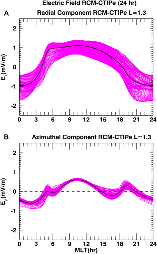
FIGURE 4. Characteristics of the (A) radial and (B) azimuthal components of the electric field projected to the magnetic equator of $L=1.3$ according to 24 h of quiet time run by the RCM-CTIPe model. The MLT variations of the electric field vary as a function of the time of the day, and they are represented every 10 min via solid magenta lines. The solid black lines represent the electric field daily averages.

3.3. Conclusion of the Experimental Analysis

The different estimates for the dawn-dusk electric potential variation at $L=1.3$ are summarized in Table 1, together with the method and the time interval considered.

TABLE 1

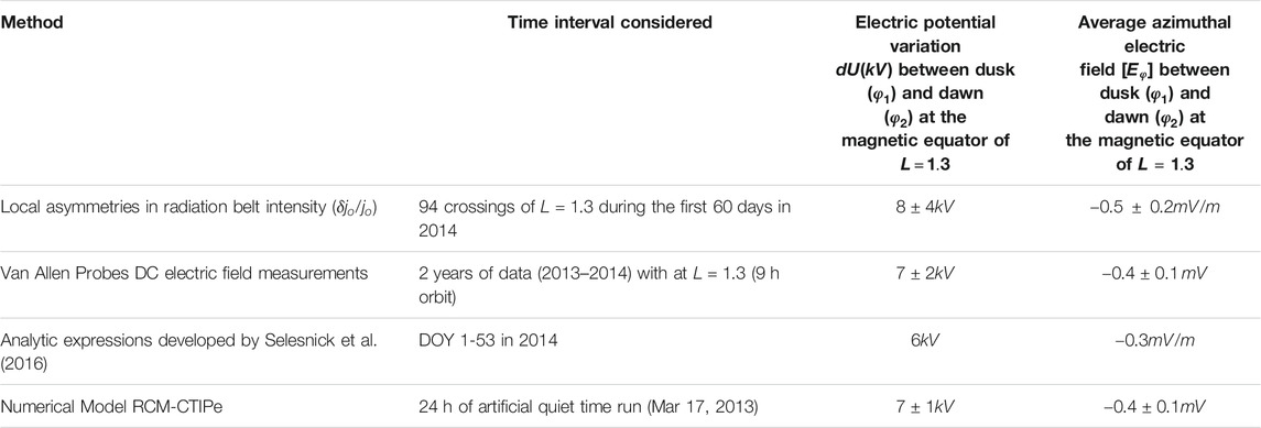
TABLE 1. Estimates of the electric potential variation between dawn and dusk, and average azimuthal electric field component between the dusk and dawn regions of the magnetic equator of $L=1.3$ according to different experimental, numerical and analytical methods.

Table 1 shows that different methods provide consistent estimates for the electric potential variation between dawn and dusk, with a magnitude of the order of 6–8 kV. The similarity is remarkable given that: 1) the neutral winds and associated wind dynamo vary from day to day and 2) every method was applied under a unique set of conditions.

An electric potential variation of 6–8 kV between dawn and dusk is ∼15 times greater than would be predicted by the usual Maynard and Chen (1975) parametrization of the Volland (1973) - Stern (1975) convection electric field model during quiet geomagnetic activity ($Kp=2$), suggesting that the solar wind-magnetosphere dynamo is unlikely to be the main of cause of the observed drift shell distortion.

Van Allen probes electric field measurements and simulations by RCM-CTIPe are in qualitative agreement, despite differences in their time intervals. These similarities confirm that the electric potential variation results mainly from the quiet time wind dynamo. Comparing Figures 3, 4 also demonstrates that the Van Allen Probes can resolve the effects of neutral winds on global electric fields.

4. Discussion: Time Variations of the Electric Potential Variation as Determined by the Measured Asymmetry in the Equatorial Electron Intensity

While the modeling and experimental results provide similar estimates for the average magnitude of the dawn-dusk electric potential variation, they do not explain the high variability revealed by the particle data analysis. The time series of dawn-dusk electric potential variation, $dU\left(t\right)$, has a standard deviation of the order of $7kV$ (Figure 2C). On the other hand, 1 day of quiet time run by RCM-CTIPe provides a standard deviation of the order of $1kV$ only, including possible longitudinal effects.

Data analyses similar to the one presented Section 3.1.1. were performed 1) using measurements by the Radiation Belt Storm Probes Ion Composition Experiment (Mitchell et al., 2013) in place of MagEIS, and/or 2) at higher $L$ values (specifically, $L=1.5$, and $L=1.7$). While quantitative analysis of RBSPICE data is incomplete, similar trends for the time variations of the dawn-dusk electric potential were observed. These findings suggest that the time variations observed correspond to real geophysical information.

We searched for possible dependencies of the time series, $dU\left(t\right),$ by performing correlation analyses with various indicators. We looked for possible correlations between the sampled electric potential variation, $dU\left(t\right)$, and the spacecraft longitudinal positions at the time, $t$, of measurements (UT). We also looked for possible variations based on a variety of indicators (presented in Figure 5), such as F10.7, Kp, Dst, and the polar cap potential, PCP, computed according to the formula by Boyle et al. (1997). We also considered substorm onsets as defined by Forsyth et al. (2015), Newell and Gjerloev (2011) and Ohtani and Gjerloev (2020). Regardless of the parameter considered, no obvious dependency was found.

FIGURE 5

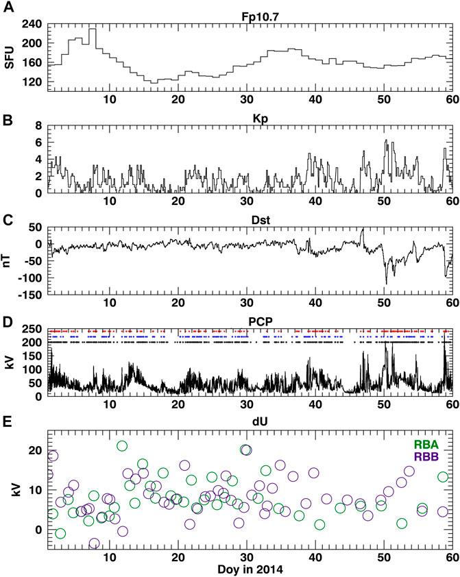
FIGURE 5. Various indicators [(A) F10.7, (B) Kp, (C) Dst and (D) Polar Cap Potential PCP] for the electromagnetic conditions associated with (E) the time dependence of the dawn-dusk electric potential variation, dU. The SuperMag substorm lists from Forsyth et al. (2015), Newell and Gjerloev (2011) and Ohtani and Gjerloev (2020) are indicated Panel (D) in black, blue and red, respectively.

Realistic modeling of the subauroral electric field evolution is required to further investigate the origin of the variability reported here.

Data Availability Statement

Publicly available datasets were analyzed in this study. This data can be found here: The Van Allen Probes electric field data are in public access in the RBSP/EFW database: www.space.umn.edu/rbspefw-data. The MagEIS and magnetic ephemeris data are available from the ECT Science Operations and Data Center, https://rbsp-ect.newmexicoconsortium.org/rbsp_ect.php Simulation outputs can be obtained by contacting NM.

Author Contributions

The first author is the lead and corresponding author. All other authors are listed in alphabetical order. We describe contributions to the paper using the CRediT (Contributor Roles Taxonomy) categories (Brand et al., 2015). Conceptualization and Funding Acquisition: SL and NM. Resources: SL, MF, NM, and RS. Methodology, Software, Validation, Formal Analysis and Investigation: SL and RS. Writing-Original Draft, Visualization and Project Administration: SL. Writing-Review and Editing: SL, RS, and MF.

Funding

SL work was performed under JHU/APL Contract No. 922613 (RBSP-EFW), NASA Grant Awards 80NSSC18K1223 and 80NSSC20K1351. RS work is supported by the Space Vehicles Directorate of the Air Force Research Laboratory.

Conflict of Interest

The authors declare that the research was conducted in the absence of any commercial or financial relationships that could be construed as a potential conflict of interest.

Publisher’s Note

All claims expressed in this article are solely those of the authors and do not necessarily represent those of their affiliated organizations, or those of the publisher, the editors and the reviewers. Any product that may be evaluated in this article, or claim that may be made by its manufacturer, is not guaranteed or endorsed by the publisher.

Acknowledgments

The authors are grateful to Seth Claudepierre, the MAGEIS team, and the RBSPICE team for insightful discussions.

References

Blake, J. B., Carranza, P. A., Claudepierre, S. G., Clemmons, J. H., Crain, W. R., Dotan, Y., Fennell, J. F., Fuentes, F. H., Galvan, R. M., George, J. S., Henderson, M. G., Lalic, M., Lin, A. Y., Looper, M. D., Mabry, D. J., Mazur, J. E., McCarthy, B., Nguyen, C. Q., O’Brien, T. P., Perez, M. A., Redding, M. T., Roeder, J. L., Salvaggio, D. J., Sorensen, G. A., Spence, H. E., Yi, S., and Zakrzewski, M. P. (2013). The Magnetic Electron Ion Spectrometer (MagEIS) Instruments Aboard the Radiation Belt Storm Probes (RBSP) Spacecraft. Space Sci Rev 179, 383–421. doi:10.1007/s11214-013-9991-8

CrossRef Full Text | Google Scholar

Boyle, C. B., Reiff, P. H., and Hairston, M. R. (1997). Empirical polar cap potentials. J. Geophys. Res. 102 (A1), 111–125. doi:10.1029/96JA01742

CrossRef Full Text | Google Scholar

Brand, A., Allen, L., Altman, M., Hlava, M., and Scott, J. (2015). Beyond authorship: attribution, contribution, collaboration, and credit. Learn. Pub. 28, 151–155. doi:10.1087/20150211

CrossRef Full Text | Google Scholar

Chau, J. L., Aponte, N. A., Cabassa, E., Sulzer, M. P., Goncharenko, L. P., and González, S. A. (2010). Quiet time ionospheric variability over Arecibo during sudden stratospheric warming events. J. Geophys. Res. 115, a–n. doi:10.1029/2010JA015378

CrossRef Full Text | Google Scholar

Echer, E., Gonzalez, W. D., and Alves, M. V. (2006). On the geomagnetic effects of solar wind interplanetary magnetic structures. Space Weather 4, a–n. doi:10.1029/2005SW000200

CrossRef Full Text | Google Scholar

Fejer, B. G. (1993). F region plasma drifts over Arecibo: Solar cycle, seasonal, and magnetic activity effects. J. Geophys. Res. 98 (A8), 13645–13652. doi:10.1029/93JA00953

CrossRef Full Text | Google Scholar

Forsyth, C., Rae, I. J., Coxon, J. C., Freeman, M. P., Jackman, C. M., Gjerloev, J., and Fazakerley, A. N. (2015). A new technique for determining Substorm Onsets and Phases from Indices of the Electrojet (SOPHIE). J. Geophys. Res. Space Physics 120 (10), 10,592. doi:10.1002/2015JA021343

CrossRef Full Text | Google Scholar

Fox, N., and Burch, J. L. (2014). “The Van Allen Probes Mission,” in Physics and Astronomy (Boston, MA: Springer). doi:10.1007/978-1-4899-7433-4

CrossRef Full Text | Google Scholar

Fuller-Rowell, T. J., Rees, D., Quegan, S., Moffett, R. J., Codrescu, M. V., and Millward, G. H. (1996). “A coupled thermosphere ionosphere model (CTIM),” in STEP: Handbook of ionospheric models. Editor R. W. Schunk (Boulder, CO: Science Communication on Solar-Terrestrial Physics), 239–279.

Google Scholar

Kletzing, C. A., Kurth, W. S., Acuna, M., MacDowall, R. J., Torbert, R. B., Averkamp, T., Bodet, D., Bounds, S. R., Chutter, M., Connerney, J., Crawford, D., Dolan, J. S., Dvorsky, R., Hospodarsky, G. B., Howard, J., Jordanova, V., Johnson, R. A., Kirchner, D. L., Mokrzycki, B., Needell, G., Odom, J., Mark, D., Pfaff, R., Phillips, J. R., Piker, C. W., Remington, S. L., Rowland, D., Santolik, O., Schnurr, R., Sheppard, D., Smith, C. W., Thorne, R. M., and Tyler, J. (2013). The Electric and Magnetic Field Instrument Suite and Integrated Science (EMFISIS) on RBSP. Space Sci Rev 179, 127–181. doi:10.1007/s11214-013-9993-6

CrossRef Full Text | Google Scholar

Imhof, W. L., and Smith, R. V. (1965). Observation of Nearly Monoenergetic High-Energy Electrons in the Inner Radiation Belt. Phys. Rev. Lett. 14, 885–887. doi:10.1103/PhysRevLett.14.885

CrossRef Full Text | Google Scholar

Lejosne, S., and Mozer, F. S. (2016a). Van Allen Probe measurements of the electric drift E × B/B 2 at Arecibo's L = 1.4 field line coordinate. Geophys. Res. Lett. 43, 6768–6774. doi:10.1002/2016GL069875

CrossRef Full Text | Google Scholar

Lejosne, S., and Mozer, F. S. (2016b). Typical values of the electric drift E × B/B 2 in the inner radiation belt and slot region as determined from Van Allen Probe measurements. J. Geophys. Res. Space Physics 121 (12), 12,014. doi:10.1002/2016JA023613

CrossRef Full Text | Google Scholar

Lejosne, S., and Mozer, F. S. (2019). Shorting Factor In‐Flight Calibration for the Van Allen Probes DC Electric Field Measurements in the Earth's Plasmasphere. Earth and Space Science 6, 646–654. doi:10.1029/2018ea000550

PubMed Abstract | CrossRef Full Text | Google Scholar

Lejosne, S., and Mozer, F. S. (2020). Inversion of the Energetic Electron "Zebra Stripe" Pattern Present in the Earth's Inner Belt and Slot Region: First Observations and Interpretation. Geophys. Res. Lett. 47, e2020GL088564. doi:10.1029/2020GL088564

CrossRef Full Text | Google Scholar

Maruyama, N., Fuller‐Rowell, T. J., Codrescu, M. V., Anderson, D., Richmond, A. D., Maute, A., et al. (2011). “Modeling the storm time electrodynamics,” in Aeronomy of the Earth's atmosphere and ionosphere, IAGA Special Sopron Book Series. Editors M. Abdu, and D. Pancheva (Dordrecht: Springer), Vol. 2. doi:10.1007/978‐94‐007‐0326‐1_35

CrossRef Full Text | Google Scholar

Mauk, B. H., Fox, N. J., Kanekal, S. G., Kessel, R. L., Sibeck, D. G., and Ukhorskiy, A. (2013). Science Objectives and Rationale for the Radiation Belt Storm Probes Mission. Space Sci Rev 179, 3–27. doi:10.1007/s11214-012-9908-y

CrossRef Full Text | Google Scholar

Maynard, N. C., and Chen, A. J. (1975). Isolated cold plasma regions: Observations and their relation to possible production mechanisms. J. Geophys. Res. 80, 1009–1013. doi:10.1029/ja080i007p01009

CrossRef Full Text | Google Scholar

McIlwain, C. E. (1961). Coordinates for mapping the distribution of magnetically trapped particles. J. Geophys. Res. 66 (11), 3681–3691. doi:10.1029/JZ066i011p03681

CrossRef Full Text | Google Scholar

Millward, G. H., Rishbeth, H., Fuller-Rowell, T. J., Aylward, A. D., Quegan, S., and Moffett, R. J. (1996). IonosphericF2layer seasonal and semiannual variations. J. Geophys. Res. 101, 5149–5156. doi:10.1029/95JA03343

CrossRef Full Text | Google Scholar

Millward, G. H., Müller-Wodarg, I. C. F., Aylward, A. D., Fuller-Rowell, T. J., Richmond, A. D., and Moffett, R. J. (2001). An investigation into the influence of tidal forcing onFregion equatorial vertical ion drift using a global ionosphere-thermosphere model with coupled electrodynamics. J. Geophys. Res. 106, 24733–24744. doi:10.1029/2000JA000342

CrossRef Full Text | Google Scholar

Mitchell, D. G., Lanzerotti, L. J., Kim, C. K., Stokes, M., Ho, G., Cooper, S., Ukhorskiy, A., Manweiler, J. W., Jaskulek, S., Haggerty, D. K., Brandt, P., Sitnov, M., Keika, K., Hayes, J. R., Brown, L. E., Gurnee, R. S., Hutcheson, J. C., Nelson, K. S., Paschalidis, N., Rossano, E., and Kerem, S. (2013). Radiation Belt Storm Probes Ion Composition Experiment (RBSPICE). Space Sci Rev 179, 263–308. doi:10.1007/s11214-013-9965-x

CrossRef Full Text | Google Scholar

Mozer, F. S. (1973). Electric fields and plasma convection in the plasmasphere. Rev. Geophys. 11 (3), 755–765. doi:10.1029/RG011i003p00755

CrossRef Full Text | Google Scholar

Newell, P. T., and Gjerloev, J. W. (2011). Substorm and magnetosphere characteristic scales inferred from the SuperMAG auroral electrojet indices. J. Geophys. Res. 116, a–n. doi:10.1029/2011JA016936

CrossRef Full Text | Google Scholar

Northrop, T. G., and Teller, E. (1960). Stability of the adiabatic motion of charged particles in the Earth's field. Phys. Rev. 117 (1), 215–225. doi:10.1103/PhysRev.117.215

CrossRef Full Text | Google Scholar

Ohtani, S., and Gjerloev, J. W. (2020). Is the substorm current wedge an ensemble of wedgelets?: Revisit to midlatitude positive bays. J. Geophys. Res. Space Physics 125, e2020JA027902. doi:10.1029/2020JA027902

CrossRef Full Text | Google Scholar

Olson, W. P., and Pfitzer, K. A. (1977). Magnetospheric magnetic field modeling, Annual Sci. Rep. contract F44620-75-C-0033, Air Force Office of Scientific Research. Huntington Beach, California: McDonnell Douglas Astronautics Co.

Pfaff, R., Rowland, D., Freudenreich, H., Bromund, K., Le, G., Acuña, M., Klenzing, J., Liebrecht, C., Martin, S., Burke, W. J., Maynard, N. C., Hunton, D. E., Roddy, P. A., Ballenthin, J. O., and Wilson, G. R. (2010). Observations of DC electric fields in the low-latitude ionosphere and their variations with local time, longitude, and plasma density during extreme solar minimum. J. Geophys. Res. 115, a–n. doi:10.1029/2010JA016023

CrossRef Full Text | Google Scholar

Pfitzer, K. A., and Winckler, J. R. (1968). Experimental observation of a large addition to the electron inner radiation belt after a solar flare event. J. Geophys. Res. 73 (17), 5792–5797. doi:10.1029/JA073i017p05792

CrossRef Full Text | Google Scholar

Reeves, G. D., Friedel, R. H. W., Larsen, B. A., Skoug, R. M., Funsten, H. O., Claudepierre, S. G., Fennell, J. F., Turner, D. L., Denton, M. H., Spence, H. E., et al. (2016). Energy‐dependent dynamics of keV to MeV electrons in the inner zone, outer zone, and slot regions. J. Geophys. Res. Space Physics 121, 397–412. doi:10.1002/2015JA021569

PubMed Abstract | CrossRef Full Text | Google Scholar

Richmond, A. D. (1989). Modeling the ionosphere wind dynamo: A review. PAGEOPH 131, 413–435. doi:10.1007/BF00876837

CrossRef Full Text | Google Scholar

Richmond, A. D., and Maute, A. (2014). “Ionospheric electrodynamics modeling,” in Modeling the ionosphere–thermosphere system. Editors J. Huba, R. Schunk, and G. Khazanov, 57–71. doi:10.1002/9781118704417.ch6

CrossRef Full Text | Google Scholar

Roederer, J. G. (1967). On the adiabatic motion of energetic particles in a model magnetosphere. J. Geophys. Res. 72 (3), 981–992. doi:10.1029/JZ072i003p00981

CrossRef Full Text | Google Scholar

Roederer, J. G., and Zhang, H. (2014). “Dynamics of Magnetically Trapped Particles,” in Foundations of the Physics of Radiation Belts and Space Plasmas, Astrophysics and Space Science Library (Berlin, Heidelberg: Springer‐Verlag). doi:10.1007/978‐3‐642‐41530‐2

CrossRef Full Text | Google Scholar

Selesnick, R. S., Su, Y. J., and Blake, J. B. (2016). Control of the innermost electron radiation belt by large‐scale electric fields. J. Geophys. Res. Space Physics 121, 8417–8427. doi:10.1002/2016JA022973

CrossRef Full Text | Google Scholar

Stern, D. P. (1975). The motion of a proton in the equatorial magnetosphere. J. Geophys. Res. 80, 595–599. doi:10.1029/ja080i004p00595

CrossRef Full Text | Google Scholar

Toffoletto, F., Sazykin, S., Spiro, R., and Wolf, R. (2003). Inner magnetospheric modeling with the Rice Convection Model. Space Sci. Rev 107, 175–196. doi:10.1007/978-94-007-1069-6_19

CrossRef Full Text | Google Scholar

Tsyganenko, N. A. (1989). A magnetospheric magnetic field model with a warped tail current sheet. Planetary and Space Science 37 (1), 5–20. doi:10.1016/0032-0633(89)90066-4

CrossRef Full Text | Google Scholar

Turner, D. L., Claudepierre, S. G., Fennell, J. F., O'Brien, T. P., Blake, J. B., Lemon, C., Gkioulidou, M., Takahashi, K., Reeves, G. D., Thaller, S., Breneman, A., Wygant, J. R., Li, W., Runov, A., and Angelopoulos, V. (2015). Energetic electron injections deep into the inner magnetosphere associated with substorm activity. Geophys. Res. Lett. 42, 2079–2087. doi:10.1002/2015GL063225

CrossRef Full Text | Google Scholar

Ukhorskiy, A. Y., Sitnov, M. I., Mitchell, D. G., Takahashi, K., Lanzerotti, L. J., and Mauk, B. H. (2014). Rotationally driven 'zebra stripes' in Earth's inner radiation belt. Nature 507, 338–340. doi:10.1038/nature13046

PubMed Abstract | CrossRef Full Text | Google Scholar

Volland, H. (1973). A semiempirical model of large-scale magnetospheric electric fields. J. Geophys. Res. 78, 171–180. doi:10.1029/ja078i001p00171

CrossRef Full Text | Google Scholar

Whipple, E. C. (1978). (U, B, K) Coordinates: A natural system for studying magnetospheric convection. J. Geophys. Res. 83 (A9), 4318–4326. doi:10.1029/JA083iA09p04318

CrossRef Full Text | Google Scholar

Wolf, R. A. (1983). “The Quasi-Static (Slow-Flow) Region of the Magnetosphere,” in Solar‐terrestrial physics: Principles and theoretical foundations. Editors R. L. Carovillano, and J. M. Forbes (Norwell, MA: D. Reidel), 303–368. doi:10.1007/978-94-009-7194-3_14

CrossRef Full Text | Google Scholar

Wolf, R. A., Spiro, R. W., Sazykin, S., and Toffoletto, F. R. (2007). How the Earth's inner magnetosphere works: An evolving picture. Journal of Atmospheric and Solar-Terrestrial Physics 69 (3), 288–302. doi:10.1016/j.jastp.2006.07.026

CrossRef Full Text | Google Scholar

Wygant, J. R., Bonnell, J. W., Goetz, K., Ergun, R. E., Mozer, F. S., Bale, S. D., Ludlam, M., Turin, P., Harvey, P. R., Hochmann, R., Harps, K., Dalton, G., McCauley, J., Rachelson, W., Gordon, D., Donakowski, B., Shultz, C., Smith, C., Diaz-Aguado, M., Fischer, J., Heavner, S., Berg, P., Malsapina, D. M., Bolton, M. K., Hudson, M., Strangeway, R. J., Baker, D. N., Li, X., Albert, J., Foster, J. C., Chaston, C. C., Mann, I., Donovan, E., Cully, C. M., Cattell, C. A., Krasnoselskikh, V., Kersten, K., Brenneman, A., and Tao, J. B. (2013). The Electric Field and Waves Instruments on the Radiation Belt Storm Probes Mission. Space Sci Rev 179, 183–220. doi:10.1007/s11214-013-0013-7

CrossRef Full Text | Google Scholar

Yamazaki, Y., and Maute, A. (2017). Sq and EEJ-A Review on the Daily Variation of the Geomagnetic Field Caused by Ionospheric Dynamo Currents. Space Sci Rev 206, 299–405. doi:10.1007/s11214-016-0282-z

CrossRef Full Text | Google Scholar