On the Saturation (or Not) of Geomagnetic Indices

Introduction

It is well known that the cross-polar-cap potential in the ionosphere “saturates” under strong driving by the solar wind (e.g., Wygant et al., 1983; Reiff and Luhmann, 1986; Weimer et al., 1990a; Myllys et al., 2017), where saturation means that the ionospheric potential is systematically lower than expected for the observed solar-wind-driving conditions. The magnitude of the polar-cap potential saturation is well described by a parameter Q ∝ v_AΣ_P (cf. Ober et al., 2003; Borovsky et al., 2009; Gao et al., 2013) (see Cross-Polar-Cap Potential Saturation section), where v_A is the Alfven speed in the unperturbed solar wind and Σ_P is the height-integrated Pedersen conductivity of the polar-cap ionosphere. When looking at a plot of a geomagnetic index as a function of the strength of a solar-wind driver function, in the strong-driving regime (which also tends to be the large-Q regime) a saturation of the index is often seen wherein the index tends to stop increasing (or shows reduced increase) as the driver strength increases.

An example of an index that saturates appears in Figure 1 where the Hp60 geomagnetic index is plotted as a function of the solar-wind driver function R_quick

${\mathrm{R}}_{\mathrm{q}\mathrm{u}\mathrm{i}\mathrm{c}\mathrm{k}}={{\mathrm{6.9}}_{\mathrm{P}}}^{1/2}{{\mathrm{n}}_{\mathrm{s}\mathrm{w}}}^{1/2}{{\mathrm{v}}_{\mathrm{s}\mathrm{w}}}^2{\sin }^2\left({\theta }_{\mathrm{c}\mathrm{l}\mathrm{o}\mathrm{c}\mathrm{k}}/2\right){{\mathrm{M}}_{\mathrm{A}}}^{-1.35}{\left[1+{{\mathrm{680M}}_{\mathrm{A}}}^{-3.30}\right]}^{-1/4}(1)$

where m_p is the mass of a proton, n_sw is the solar-wind proton number density, θ_clock is the IMF clock angle with respect to the Earth’s dipole, and M_A = v_sw/v_A is the solar-wind Alfven Mach number, which is a function of v_sw, B_sw, and n_sw. The values of R_quick are constructed using the 1-h-resolution OMNI2 solar-wind data set (King and Papitashvili, 2005). Hp60 is essentially the Kp index with a 60-min time resolution rather than a 3-h time resolution. Hp60₁ is Hp60 with a 1-h time lag from the solar wind. Like Kp (Thomsen, 2004), Hp60 is a measure of the internal convection in the magnetosphere. R_quick is the quick (simplified) derivation of the Cassak-Shay reconnection-rate equation (Cassak and Shay, 2007; Borovsky, 2008) applied at the nose of the magnetosphere written in terms of upstream solar-wind parameters (Borovsky and Birn, 2014; Borovsky and Yakymenko, 2017). The full derivations (Borovsky, 2008, 2013) produce more-accurate driver functions but result in algebraically much-more-complicated driver functions. Each orange point and each black point in Figure 1 represents 1 h of data from the years 1995–2004 and the blue points are 21-point running averages of the orange points. (To spread the orange points vertically so that they do not lie on discrete lines, a small random value has been added to Hp60₁ when it is plotted as the black points.) Over the range of the 50th–90th percentiles of the R_quick values a least-squares linear-regression fit is made to the hourly values (black points) of Hp60₁ as a function of R_quick and that line is plotted in red. The line is extended to large R_quick values. The running average shows the vertical-versus-horizontal trend underlying the orange points: note for strong driving (large R_quick) that the running average flattens out instead of following the linear-regression fit: this is an example of a geomagnetic index saturating. In this report saturation of an index will be indicated by the index having a not-linear behavior going from mid-range driving to the strongest driving with the strength of the index weakening: this will be indicated by comparing the red-line fit for mid-range driving with the blue 21-point running averages going into the strongest driving.

FIGURE 1

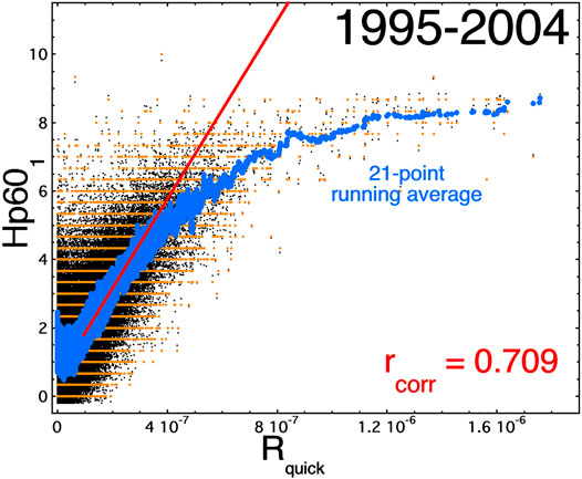
FIGURE 1. The 1-h -lagged Hp60 index is plotted as a function of R_quick for the years 1995–2004. The orange points are the HP60 index and the black points are the HP60 index with small random numbers added to spread the points off the lines. Each orange point and each black point is 1 h of data. The blue points are 21-point running averages of the orange points. The thick red line is a least-squares linear-regression fit to Hp60₁ over the 50th–90th percentile of the R_quick values, and the red line is extended to larger R_quick values. The Pearson linear correlation coefficient r_corr between Hp60₁ (orange points) and R_quick is indicated in red.

Note that throughout this paper, 21-point running averages of the data will be plotted, as in Figure 1, with the unaveraged data typically not plotted. The 21-point running averages are to guide the eye about trends (such as bends) in the underlying un-averaged data. Often the trend in the data is not discernable on a plot without the running average. To obtain the 21-point running averages the data is sorted according to the magnitude of the driver-function value (horizontal axis) and then the running average is performed on the index (vertical axis). Hence, each point of the running average is the average value of the index for the 21 values of the driver function that are the closest in magnitude. 21 points was chosen as a compromise. With much more that 21 points, the running average curve does not extend into the strong-driving region of the plot. With much less than 21 points there is no advantage to averaging the data since the averaging curve will be as noisy as the underlying data. Note also that whenever correlations, etc., are calculated, they are calculated using the un-averaged data.

One motivation for investigating the nature of geomagnetic-index saturation is the development of composite geomagnetic indices (Borovsky and Denton, 2018; Borovsky and Osmane, 2019) that do not exhibit saturation at strong driving, even though some of the geomagnetic indices used to create the composite indices do exhibit saturation.

In the investigation of geomagnetic-index saturation, this paper will explore questions about 1) whether the nature of the index matters (what it measures and how it is measured), 2) the relation of index saturation to polar-cap potential saturation, and 3) the role of the choice of the solar-wind driver function.

Cross-Polar-Cap Potential Saturation

Several mechanisms have been suggested for the cause of the saturation of the cross-polar-cap potential (cf. reviews by Borovsky et al., 2009; Gao et al., 2013; Myllys et al., 2017), but there is no community consensus as to which of the mechanisms is correct or dominant.

The reduction of the cross-polar-cap potential can be expressed as a multiplicative factor (1+Q)⁻¹ (Lavraud and Borovsky, 2008) where Q is a dimensionless parameter. Two physical arguments about polar-cap saturation lead to essentially the same formula for Q. Both arguments concern the solar wind, the magnetopause, and the polar-cap (open-field-line) ionosphere. First, Siscoe et al. (2004) argue that the high-latitude magnetopause current closes across the polar-cap ionosphere and that the magnetopause current is limited in magnitude by the amount of j×B force needed to halt the ram pressure of the solar wind. That derivation (Eqs 1–3 in Siscoe et al. (2004) with ξ = 3.5) yields

$\mathrm{Q}={\mathrm{V}}_{\mathrm{A}}{\mathrm{\sum }}_{\mathrm{p}}/892(2)$

where v_A is the Alfven speed in the unperturbed solar wind in units of km/s and Σ_P is the height-integrated Pedersen conductivity of the polar-cap ionosphere in units of mho. Second, in a current-starvation (Alfven wing) argument (Goertz and Boswell, 1979; Kivelson and Ridley, 2008), to apply a potential ϕ across the polar cap a Pedersen current proportional to the Pedersen conductivity Σ_P must be supplied from field-aligned currents, with those field-aligned currents supplied to the polar cap by the solar-wind plasma. That parallel current is fed by an ion-polarization-drift current in the solar wind plasma. The Alfven speed of a plasma is governed by the strength of the ion-polarization-drift current (Nicholson, 1983), so the supply of parallel current is limited and proportional to v_A⁻¹. Hence the parameter

$\mathrm{Q}={\mathrm{V}}_{\mathrm{A}}{\mathrm{\sum }}_{\mathrm{p}}/795(3)$

[Eq. 23 of Goertz and Boswell (1979)] describes the potential reduction of the polar cap caused by the inability of the solar wind to supply the required Pedersen current. Both arguments lead to essentially the same formula for Q since they both argue that the magnetopause current connects to the cross-polar-cap current: in the second argument the ion-polarization drift in the solar wind is the Alfvenic rotational discontinuity of the magnetopause propagating into the solar-wind plasma.

Note that large Q values tend to occur for low-Mach-number solar wind (Lavraud and Borovsky, 2008) where low values of the Alfven Mach number M_A = v_sw/v_A are produced by high values of v_A. Low-Mach-number solar wind corresponds to the passage of a magnetic cloud (Borovsky and Denton, 2006).

Saturation and the Nature of the Geomagnetic Index

In exploring why (or why not) a geomagnetic index saturates, it is suggested that the cause of the saturation could be 1) nature of the index, 2) a relation to cross-polar-cap potential saturation, or 3) the use of the wrong driver function or an incomplete driver function. The nature of the index is what activity in the magnetosphere-ionosphere system the index measures and how the index measures that activity.

An example of how an activity is measured appears in Figure 2, where the auroral-electroject indices AE and SME are explored. Both AE and SME are indices that measure the intensity of the auroral-electrojet current; AE is measured with a modest number of ground magnetometer stations located in a ring around the Earth at high (northern) latitudes (Davis and Sugiura, 1966) whereas the SuperMAG SME is measured with a large network of ground magnetometer stations over a rang of latitudes (Newell and Gjerloev, 2011; Bergin et al., 2020). Both the nightside and the dayside auroral zones map into closed field regions within the magnetosphere (cf. Feldstein and Galperin, 1985; Frey et al., 2019). It is well known that the AE index saturates under strong driving (Weimer et al., 1990a,b). In the panels (a) and (b) of Figure 2 the AE₁ and SME₁ (1-h lagged from the solar wind) indices in the years 1995–2004 are plotted as functions of the Newell driver function Φ_Newell

${\mathrm{\Phi }}_{\mathrm{N}\mathrm{e}\mathrm{w}\mathrm{e}\mathrm{l}\mathrm{l}}={{\mathrm{V}}_{\mathrm{s}\mathrm{w}}}^{4/3}{{\mathrm{B}}_{\mathrm{\perp }}}^{2/3}{\sin }^{8/3}({\mathrm{\theta }}_{\mathrm{c}\mathrm{l}\mathrm{o}\mathrm{c}\mathrm{k}}/2)(4)$

FIGURE 2

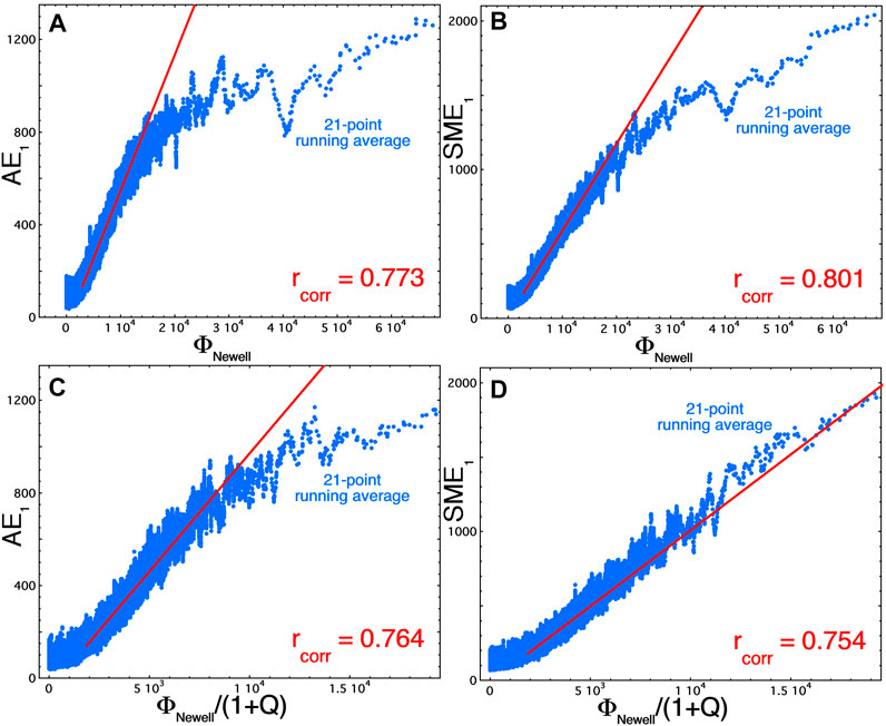
FIGURE 2. For the years 1995–2004, the 1-h-lagged AE and SME indices are plotted as functions of the Newell driver function Φ_Newell. The blue points are 21-point running averages of the (unplotted) 1-h values. The red lines are a least-squares linear-regression fits over the 50th–90th percentile of the driver-function values, and the red lines are extended to larger driver-function values.

(Newell et al., 2007). Only the 21-point running averages (blue) of the hourly points are plotted in the four panels, along with a least-squares linear-regression fit to the hourly points in the 50th–90th percentile range of the driver function Φ_Newell (red). Panel (a) is AE₁ versus Φ_Newell: the 21-point running average shows a very strong saturation (flattening) for large values of Φ_Newell. Panel (b) is SME₁ versus Φ_Newell: SME₁ in panel (b) shows much less saturation than does AE₁. In each panel of Figure 2 the Pearson linear-correlation coefficient r_corr for all 1-h data points is noted in red. Note higher Pearson linear correlation coefficients r_corr for SME₁ than for AE₁. Cross-polar-cap potential saturation can be largely corrected (mathematically accounted for) by dividing the solar-wind driver function by (1+Q) (Ober et al., 2003; Borovsky et al., 2009). In panels (c) and (d) of Figure 2 the driver function Φ_Newell/(1+Q) is used to correlate with AE₁ and with SME₁. Here, Q is calculated as Q = v_AΣ_P/795 with Σ_P = 0.77 F_10.7^1/2 (Ober et al., 2003). Comparing panels (a) and (c) it is seen that dividing the solar-wind driver by (1+Q) does not fully account for the observed saturation of AE₁, but comparing panels (b) and (d) it is seen that dividing the solar-wind driver by (1+Q) pretty much fully accounts for the saturation of SME₁. Hence, the saturation of AE appears to be in part related to the cross-polar-cap potential saturation plus another effect, whereas the milder saturation of SME appears to be solely related to the cross-polar-cap potential saturation. The additional saturation of AE may be caused by the fact that when driving is very strong the auroral oval expands to lower latitudes (e.g., Gussenhoven et al., 1983; Penskikh et al., 2021) away from the high-latitude ring of AE magnetometer stations, reducing the magnetic perturbations measured by those stations. The more-extensive network of SuperMAG ground magnetometer stations apparently does not suffer from this deficiency (cf. Bergin et al., 2020).

Note in Figure 2 that dividing the solar-wind driver by (1+Q) helps to eliminate the appearance of saturation at strong driving, however it typically reduces the overall (all-points) linear correlation coefficient r_corr between the index and the solar-wind driver function.

The saturation of the auroral-electrojet indices is further explored in Figure 3 where the behavior of the AU and AL indices is compared with the behavior of the SuperMAG SMU and SML indices. The solar-wind driver function used is R_quick [expression (1)]. The auroral-electrojet index AE is the sum of two other indices AE = AU − AL where AU is predominantly a positive number and AL is predominantly a negative number. AL is the maximum intensity of the eastward auroral electrojet and AU is the maximum intensity of the westward auroral electrojet: typically AL is recorded on the nightside of the auroral oval and typically AU is recorded on the dayside of the auroral oval (e.g., Goertz et al., 1993). The blue curve in Figure 3A is the 21-point running average of hourly values from the years 1995–2004 of -AL₁ (1-h lagged) and of AU₁ (1-h lagged) in Figure 3B. The red line in both panels is a least-squares linear-regression fit to the hourly values in the 50th–90th percentile range of R_quick. In Figure 3A it is seen that the AL index saturates, but note in Figure 3B that fractionally the AU index saturates much more strongly. The green curves in Figure 3 are the 21-point running averages for the SuperMAG SML₁ index [panel (a)] and for the SuperMAG SMU₁ index [panel (b)]. Note that SML and SMU saturate less than AL and AU do. Presumably the stronger saturations of AL and AU are caused by the equatorward expansion of the auroral oval away from the ring of high-latitude stations that measure AL and AU. Note in the two panels of Figure 3 the higher correlation coefficients r_corr between the indices SML and SMU with R_quick versus of coefficients between AL and AU with R_quick.

FIGURE 3

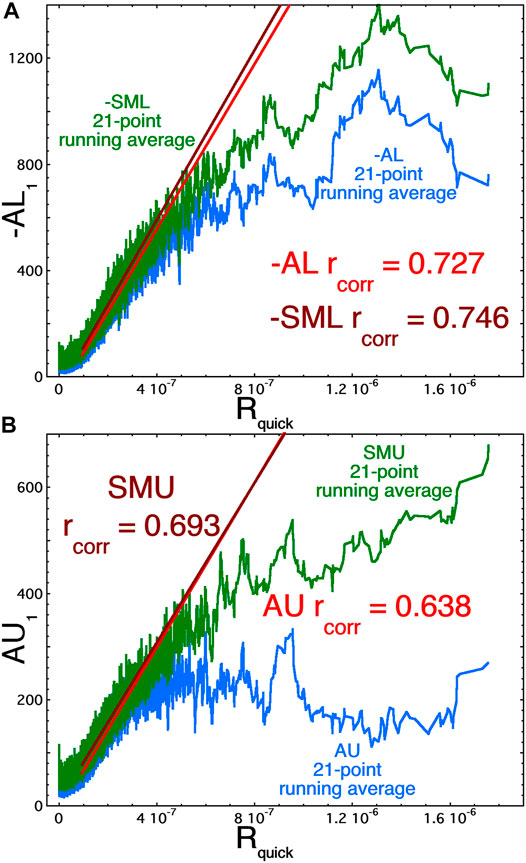
FIGURE 3. For the years 1995–2004, the -AL index [panel (A)] and the AU index [panel (B)] are plotted as a function of R_quick. The blue points are 21-point running averages of the (unplotted) 1-h values. The red lines are a least-squares linear-regression fits over the 50th–90th percentile of the R_quick values, and the red lines are extended to larger R_quick values.

In Figure 4 the behavior of 8 geomagnetic indices with respect to the magnitude of the solar-wind driver function R_quick is examined. With the exception of PCI in panel (c), the other 7 indices are associated with processes internal to the magnetosphere. In each panel of Figure 4 the 21-point running average of the individual 1-h data points are plotted (blue) along with a least-squares linear-regression fit (red) to the individual points in the 50th–90th percentile range of R_quick. Saturation of an index will appear as a decrease of the slope of the running average as the magnitude of R_quick increases. In Figures 4A,B it is seen that the planetary range index am (cf. Mayaud, 1980) (1-h lagged from the solar wind) and the Dst index (2-h lagged from the solar wind) do not saturate under the action of the R_quick driver. Figure 4C indicates that the polar cap index PCI (Troshichev et al., 1988) (no time lag from the solar wind) saturates only mildly, i.e., its slope decreases by it does not flatten (See also Weimer et al., 2017 for no saturation of the field-aligned currents feeding the polar cap.). Similarly, the index of the mean electron precipitation mPe (Emery et al., 2009) (1-h lagged from the solar wind) only saturates mildly in Figure 4D. The midnight boundary index MBI (Gussenhoven et al., 1983) (1-h lagged from the solar wind) in Figure 4E and the Kp index (1-h lagged from the solar wind) in Figure 4F both show strong saturation for the R_quick driver function. In Figures 4G,H S_grd and S_geod are detrended ULF indices from ground (gr) measurements and from geosynchronous-orbit (geo) measurements (Romanova et al., 2007; Kozyreva et al., 2007; Romanova and Pilipenko, 2009), with the detrending described in Borovsky and Denton (2014). S_grd and S_geod show strong saturation. Note that although am, MBI, and Kp are all measures of the strength of magnetospheric convection, am does not saturate while MBI and Kp do saturate.

FIGURE 4

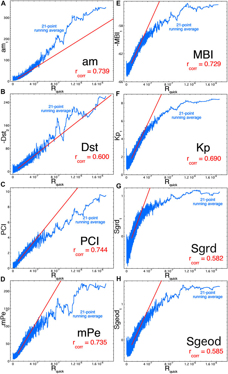
FIGURE 4. For the years 1995–2004, eight geomagnetic indices are plotted as a function of R_quick. Hourly. The blue points are 21-point running averages of the (unplotted) 1-h values. The red lines are a least-squares linear-regression fits over the 50th–90th percentile of the R_quick values, and the red lines are extended to larger R_quick values.

Index Saturation and the Solar-Wind Driver Function

In Figure 5 the saturation of the 1-h-lagged SuperMAG SME₁ index is examined for 5 different solar-wind driver functions. In each panel of Figure 5 the blue curve is the 21-point running average of the individual 1-h data points for the years 1995–2004 and the red line is a least-squares linear-regression fit to the individual 1-h data points in the 50th–90th percentile range of the driver strength. In each panel the Pearson linear correlation coefficient r_corr is indicated in red. In Figure 5A SME₁ is plotted as a function of the driver function v_swB_south, which is v_swB_south = −v_swB_z for B_z (GSM coordinates) southward (negative) and v_swB_south = 0 for B_z northward (positive). The blue curve in Figure 5A indicates a very strong saturation at large values of v_swB_south. Figure 5B examines SME₁ as a function of the Newell driver function Φ_Newell [expression (4)]: for Φ_Newell the degree of saturation of SME₁ is less dramatic than the saturation under v_swB_south in Figure 5A. Figure 5C examines SME₁ as a function of the reconnection driver function R_quick: again, the saturation for R_quick is less than the saturation for v_swB_south in Figure 5A. There are a number of solar-wind driver functions that have functional forms that seem unphysical in terms of the suspected physical processes by which the solar wind drives the Earth’s magnetosphere (cf. Borovsky, 2014): v_sw + 75B_swsin²(θ_clock/2) (where v_sw is in units of km/s and B_sw is in units of nT) is one of them. In Figure 5D the reaction of SME₁ to the solar-wind driver function v_sw + 75B_swsin²(θ_clock/2) is plotted: the deviation of the 21-point running average (blue) from the linear regression (red) commences at higher values of the driver function than in panels (a)–(c). Hence, the saturation of SME₁ to the driver v_sw + 75B_swsin²(θ_clock/2) only occurs at the highest values of the driver function. Figure 5E displays the relation between SME₁ and the canonical solar-wind driver function S_(1)(9b), which is a composite of multiple solar-wind variables given by Eq. 9b of Borovsky and Denton (2014) [and see expression (5b) below]. As can be seen in Figure 5E, there is little or no saturation of SME₁ under solar-wind driving described by S_(1)(9b).

FIGURE 5

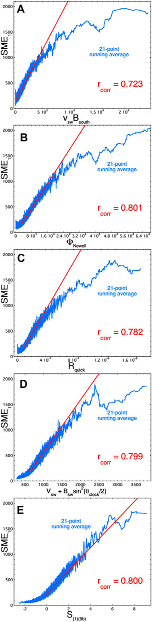
FIGURE 5. For the years 1995–2004, the 1-h-lagged SME index is plotted as a function of five different solar-wind driver functions. The blue points are 21-point running averages of the (unplotted) 1-h values. The red lines are a least-squares linear-regression fits over the 50th–90th percentile of the driver-function values, and the red lines are extended to larger driver-function values.

New composite geomagnetic indices are possible derived with the use of canonical correlation analysis (vector-vector correlation) (Borovsky, 2014, 2020a; Borovsky and Denton, 2014, 2018; Borovsky and Osmane, 2019). The technique reduces a multidimensional time-dependent solar-wind state vector and a multidimensional time-dependent magnetospheric-system state vector to a time-dependent driver scalar and a time-dependent magnetospheric scalar (a composite index), with the composite index describing the global response of the magnetospheric system to the solar wind. The magnetospheric state vector contains multiple measures of the magnetospheric system, typically multiple geomagnetic indices plus spacecraft measurements of the states of various magnetospheric particle populations. This system description that is a reduction from the state vectors has advantages: compactness, low noise, and high prediction efficiency. Most important for the present study, the composite index shows linearity in the description of the magnetospheric system response to the solar-wind driver. I.e., the composite magnetospheric scalar does not exhibit saturation at strong driving by its matching composite scalar solar-wind driver. Here we will examine a case when only multiple geomagnetic indices are used in the magnetospheric state vector. The example is shown in Figure 6, where the composite magnetospheric scalar E_(1)(9a)(t) (“E” representing Earth) is plotted as a function of its solar-wind driver scalar S_(1)(9b)(t). The formula to create E_(1)(9a) from 9 geomagnetic indices and the formula to create S_(1)(9b) from 9 solar-wind variables are given by Eqs 9a, 9b of Borovsky and Denton (2014), which are repeated here:

$\begin{array}{l}{E}_{\left(1\right)\left(9\mathrm{a}\right)}=0.176\log {\left({\mathrm{AE}}_1\right)}^{\ast }+0.036{{\mathrm{AU}}_1}^{\ast }+0.03{{\mathrm{Al}}_1}^{\ast }+0.244{{\mathrm{PCI}}_1}^{\ast }\\ +0.166{{\mathrm{KP}}_1}^{\ast }-0.235{{\mathrm{MBI}}_1}^{\ast }-0.236{{\mathrm{Dst}}_1}^{\ast }+0.057{S_{\mathrm{g}\mathrm{r}\mathrm{d}1}}^{\ast }\\ +0.048{S_{\mathrm{g}\mathrm{o}\mathrm{d}1}}^{\ast }\end{array}(\mathrm{5a})$

$\begin{array}{l}{S}_{\left(1\right)\left(9\mathrm{b}\right)}=0.725\log {\left({\mathrm{n}}_{\mathrm{s}\mathrm{w}}{\mathrm{v}}_{\mathrm{s}\mathrm{w}}^2\right)}^{\ast }-0.535\log {\left({\mathrm{n}}_{\mathrm{s}\mathrm{w}}\right)}^{\ast }-0.357{B_z}^{\ast }+0.274{\langle {\sin }^2\left({\mathrm{\theta }}_{\mathrm{c}\mathrm{l}\mathrm{o}\mathrm{c}\mathrm{k}}/2\right)\rangle }_{{\mathrm{3}}^{\ast }}\\ +0.233{\displaystyle \int {}^{22hr}{{\displaystyle \mathrm{R}}}_{\mathrm{q}\mathrm{u}\mathrm{i}\mathrm{c}\mathrm{k}}\mathrm{d}{\mathrm{t}}^{\ast }}+0.189{{\mathrm{B}}_{\mathrm{s}\mathrm{w}}}^{\ast }+0.087{\langle {\mathrm{\theta }}_{\mathrm{B}\mathrm{n}}\rangle }_{{\mathrm{3}}^{\ast }}\\ -0.070\log {\left({\mathrm{M}}_{\mathrm{A}}\right)}^{\ast }+0.064\log {\left({\mathrm{F}}_{10.7}\right)}^{\ast }\end{array}(\mathrm{5b})$

FIGURE 6

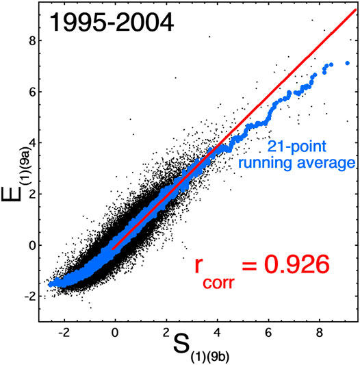
FIGURE 6. For the years 1995–2004, the composite geomagnetic index E_(1)(9a) is plotted as a function of the composite solar-wind driver function S_(1)(9b). The black points are 1-h values and the blue points are 21-point running averages of the black points. The red lines are a least-squares linear-regression fits over the 50th–90th percentile of the S_(1)(9b) values, and the red lines are extended to larger S_(1)(9b) values.

The asterisks in expressions (5a) and (5b) mean that the variable is standardized (mean value subtracted off followed by division by the standard deviation) and the numerical subscripts are the hrs of time lag of the magnetospheric variables from the solar-wind variables. Since the variables are standardized, either the base-e or the base-10 logarithms can be used. In expression (5b) the term ∫ ^22 h R_quick dt is a 22-h time integral (into the past) of the reconnection driver function R_quick; this term in S₍₁₎ represents the past history of driving geomagnetic activity and acts to correct a slight hysteresis in the solar-wind driving of the magnetosphere (which might be an atmospheric flywheel effect (e.g., Richmond and Matsushita, 1975). In Figure 6 the hourly points of E_(1)(9a) as a function of S_(1)(9b) for the years 1995–2005 are plotted in black, a 21-point running average of the black points is plotted in blue, and a least-squares linear-regression fit to the black points in the 50th–90th percentile range of S_(1)(9b) is plotted in red. Note the b) ely high Pearson linear correlation coefficient of 0.926 between E_(1)(9a) and S_(1)(9b). Figure 6 shows the linearity for all strengths of the driving, with the running average (blue) tracking the linear fit (red). Note that other E₍₁₎ and S₍₁₎ variables composed of other geomagnetic indices and other solar-wind variables (with and without a ∫R_quickdt term) also show linearity in the response (no saturation): c.f. Figure 1 of Borovsky (2014), Figure 2A of Borovsky and Denton (2018), and Figure 1 of Borovsky and Osmane (2019). Note that the variable F_10.7 (which is used to construct a Q value) is not used in the S₍₁₎ values for these three referenced figures [cf. Eq. 2a of Borovsky (2014), Eq. 8 of Borovsky and Denton (2018), and Eq. 1a of Borovsky and Osmane (2019)], hence the lack of saturation in these cases is not dependent on the ability of the solar-wind driver function to know the value of Q.

An obvious question about the composite magnetospheric index E_(1)(9a) is: How does the composite magnetospheric index E_(1)(9a) behave in reaction to other solar-wind driver functions besides S_(1)(9b)? This is explored in Figure 7 for four other driver functions. In Figures 7A–D of the reaction of E_(1)(9a) to the solar-wind drivers v_swB_south, Φ_Newell, R_quick, and v_sw + 75B_swsin²(θ_clock/2) are examined by plotting the 21-point running averages (blue) of the hourly data points for the years 1995–2004 and comparing with linear-regression fits (red) in the 50th–90th percentile range of each driver function. In all four panels (a)–(d) the running averages indicate a saturation of E_(1)(9a) for the four driver functions at strong levels of driving. In Figures 7E–H the four driver functions are each divided by (1+Q): this appears to more-or-less correct (or overcorrect) for the strong-driving saturation of E_(1)(9a) for the four driver functions.

FIGURE 7

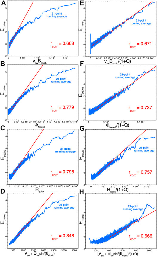
FIGURE 7. For the years 1995–2004 the composite geomagnetic index E_(1)(9a) is plotted as a function of four solar wind driver functions (left column) and as a function of the same driver functions divided by the factor (1+Q) (right column). The blue points are 21-point running averages of the (unplotted) 1-h values. The red lines are a least-squares linear-regression fits over the 50th–90th percentile of the driver-function values, and the red lines are extended to larger driver-function values.

Comparing Figure 6 for driver S_(1)(9b) where there is no saturation with Figures 7A–D with other drivers where there is saturation, it seems that S_(1)(9b) compensates for saturation (This is also the case in Figure 5). This implies that S_(1)(9b) has the (1+Q) information in it. However, F_10.7 was not one of the solar-wind variables used to derive S_(1)(9b) [see expression (5b)] and none of the other solar-wind variables in expression (5b) would seem to serve as a good proxy for F_10.7.

Figures 8, 9 examines the relation of the composite solar-wind driver function S_(1)(9b) to 12 geomagnetic indices (similar to Figures 3, 4 for R_quick and various indices). With the exception of PCI in panel (c), all geomagnetic indices in Figure 8 pertain to processes internal to the magnetosphere-ionosphere system. In each panel of Figure 8 the blue curve is a 21-point running average of the 1-h data points and the red line is a linear-regression fit to the index as a function of S_(1)(9b) in the 50th–90th percentile range of the S_(1)(9b) values (with the red line extended to larger S_(1)(9b) values). Comparing Figure 8 with Figures 3, 4 it is seen that S_(1)(9b)compensates for the strong-driving saturation of indices more than R_quick does. At strong driving S_(1)(9b) reduces the saturation of PCI, mPe, MBI, Kp, SML, SMU, S_grd and S_geod. S_(1)(9b) tends to overcompensate at strong driving for the indices am and Dst. Note that the all-points Pearson linear correlation coefficients are much higher for S_(1)(9b) and the indices in Figure 8 than they are for R_quick and the indices in Figures 3, 4. Note also in comparing the 21-point running averages of Figure 8 with the running averages of Figures 3, 4 that S_(1)(9b) tends to introduce a nonlinearity at weak driving, with the index values being larger than a linear trend between S_(1)(9b) and the index.

FIGURE 8

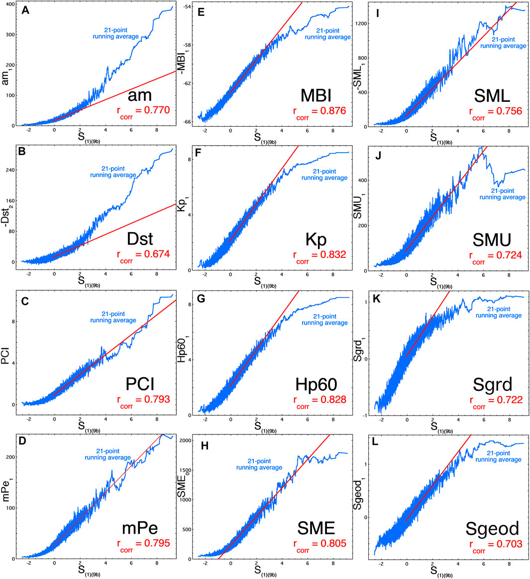
FIGURE 8. For the years 1995–2004, 12 geomagnetic indices are plotted as a function of the composite driver function S_(1)(9b). The blue points are 21-point running averages of the (unplotted) 1-h values. The red lines are a least-squares linear-regression fits over the 50th–90th percentile of the S_(1)(9b) values, and the red lines are extended to S_(1)(9b) values.

FIGURE 9

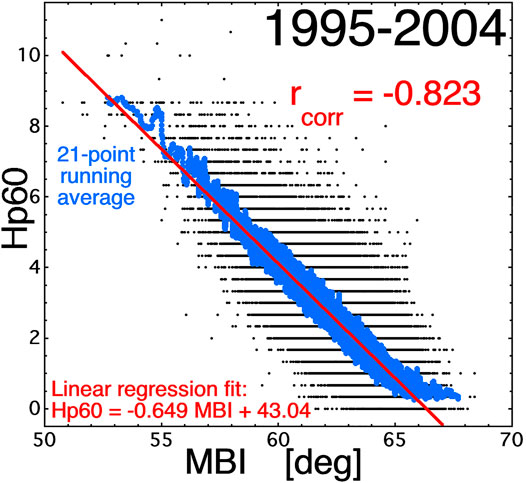
FIGURE 9. For the years 1995–2004 the Hp60 index is plotted as a function of the MBI index (black points). A 21-point running average of Hp60 is plotted as the blue points and a linear-regression fit to the black points is plotted as the red line.

Summary and Discussion

In this report some simple observations were made about the reactions of several geomagnetic indices to several solar-wind driver functions with the focus on whether or not the indices exhibit saturation for strong driving. Those observations are summarized as follows.

1) In plotting the strength of a geomagnetic index I(t) as a function of the strength of the solar-wind driver function D(t) and paying attention to the slope d|I|/dD of |I| as a function of the strength of D, saturation of the index is a reduction of the slope going from the region of moderate driving to the region of very strong driving.

2) Different geomagnetic indices show different degrees of saturation. E.g., for the solar-wind driver function R_quick the indices am and Dst show no saturation, the PCI index shows mild saturation, and the indices mPe, MBI, Kp, Hp60, AE, AL, and AU show strong saturation.

3) Using the SuperMAG auroral-electrojet indices SME, SML, and SMU reduces the saturation seen with the AE, AL, and AU auroral-electrojet indices.

4) The degree of saturation of a geomagnetic index depends on the solar-wind driver function used.

5) Dividing a driver function by the theoretical polar-cap-saturation function (1+Q) can sometimes compensate the saturation of an index at strong driving, although sometimes it overcompensates. Although the derivations of Q are based on solar-wind/ionosphere arguments, the Q factor often compensates for geomagnetic indices that are associated with internal magnetospheric processes. The linear correlation coefficient between the index and the driver function often decreases when the driver function is divided by (1+Q), even in cases when saturation at high-driving is successfully corrected.

6) Derived composite indies E₍₁₎ do not exhibit saturation with their composite solar-wind driver functions S₍₁₎. E₍₁₎ does saturate under other solar-wind driver functions (e.g., v_swB_south, Φ_Newell, R_quick) and dividing those driver functions by (1+Q) tends to compensate for the saturation of E₍₁₎.

7) The discussion subsections below concern difficulties in determining the strength of the driving of the magnetosphere by the solar wind and the difficulties in measuring the reaction of the magnetosphere-ionosphere system to that driving. Those discussions can be summarized as follows. The strength of the driving of the magnetosphere-ionosphere system by the solar wind is difficult to quantify and there is a lack of quantification of physical processes ongoing in the system’s reaction to the solar-wind driving. We have predictions of the driving strength (via solar-wind driver functions) and proxy measurements of physical processes (via geomagnetic indices). Working with these indirect predictions and proxies make the causes of saturation difficult to interpret.

8) Two unsolved issues are: 1) Why is the saturation of various geomagnetic indices related to cross-polar-cap potential saturation? 2) Why are some composite solar-wind driver functions S₍₁₎ able to compensate for saturation without access to F_10.7 or other variables that would predict ionospheric conductivity?

Driving of the Magnetosphere-Ionosphere System

There is much that is not understood about the coupling of the solar wind to the Earth’s magnetosphere and about the resulting driving of magnetospheric activity (e.g., Borovsky, 2021). Two important questions here are: 1) What do we mean by strength of driving? and 2) How do we measure the strength of driving?

We imagine that the total dayside reconnection rate (total amount of magnetic flux reconnected per unit time) would be a good indicator of the strength of driving of the magnetosphere by the solar wind. As of yet, we have no way of measuring the total dayside reconnection rate, we can only predict the rate from a knowledge of solar-wind parameters via the use of a variety of solar-wind driver functions.

The reconnection-rate function R_quick derived from the Cassak-Shay reconnection-rate equation is incomplete. R_quick only applies at the nose of the magnetosphere. To get the total reconnection rate along the entire dayside reconnection line we need the magnetospheric and magnetosheath plasma and field parameters along the entire reconnection line, which among other things requires a knowledge of where on the magnetopause the reconnection line is. Additionally, an accounting is needed for the effects of magnetosheath-magnetosphere velocity shear on the local reconnection rate. Also, we are completely lacking systematic information about the magnetospheric-plasma mass density ρ_mag at the dayside magnetosphere (Borovsky et al., 2013), which is in the denominator of the Cassak-Shay equation. And if we knew all that, we would still have only a prediction of the total reconnection rate, not an actual measurement.

Borovsky and Birn (2014) (see also Borovsky et al., 2008) argue that the concept of the solar-wind motional electric field controlling the dayside reconnection rate is mistaken (But see Lopez, 2016 for a response to this argument). The dayside reconnection rate has the dimensions of an electric field and for decades it has been assumed that reconnection electric field is proportional to the solar-wind motional electric field (e.g., Gonzalez and Mozer, 1974; Kan and Lee, 1979; Gonzalez and Gonzalez, 1981; Sergeev and Kuznetsov, 1981): reconnection simulations by Birn and Hesse (2007) directly demonstrated that the two electric fields are not related.

Using global MHD simulation codes can be helpful for measuring the strength of driving, but the design of the simulation numerical scheme must guarantee that the MHD code gets the reconnection rate correct (cf. Borovsky et al., 2008).

A direct measure of the total dayside reconnection rate is the total ionospheric plasma flow (with ionospheric magnetic field) crossing the dayside open-closed boundary in the ionosphere: however, discerning where exactly that open-closed boundary is in ionospheric radar flow maps is difficult. Another measure of the total dayside reconnection rate is via the cross-polar-cap potential, however that cross-polar-cap potential is also affected by the nightside reconnection rate (Cowley and Lockwood, 1992) and there can be time delays between the reconnection rate and the polar-cap potential (Siscoe et al., 2011).

Note also that the assumption that the total dayside reconnection rate is a measure of the driving is ignoring any viscous driving of the magnetosphere by the solar wind (e.g., Lockwood and Moen, 1999; Farrugia et al., 2001), and questions about how to measure (Mozer, 1984; Drake et al., 2009) or predict (Vasyliunas et al., 1982; Borovsky, 2013) that portion of the driving.

Measuring the Reaction of the Magnetosphere-Ionosphere System to Driving

To understand quantitatively the reaction of the magnetosphere-ionosphere system to the solar wind, direct measures of the strengths of various magnetospheric physical processes is desirable. Instead we typically have proxy measures (e.g., geomagnetic indices) of diverse current systems.

One direct measure that we do have of a physical process is the cross-polar-cap potential in the ionosphere: however, as mentioned above that potential is affected by solar-wind driving and by reconnection in the magnetotail. Another physical quantity to focus on is the strength of magnetospheric convection, but a difficulty is directly measuring the strength of that convection. Specifically the total rate of convection might be defined as the amount of magnetic flux carried at the E-cross-B drift speed from the nightside magnetosphere into the dayside magnetosphere. The low-latitude-boundary-layer flow of flux antiSunward would not be included in that measure: that flow would be a measure of the driving in addition to the dayside reconnection rate. But there would be a difficulty in directly measuring the total convection rate in the magnetosphere with a limited number of spacecraft: a local measure of E-cross-B would need to be put into the context of the estimated time-dependent morphology of the magnetosphere to get a total convection from a local convection. Ionospheric radar convection maps may be a promising option.

Expectation of a Linear Reaction to Driving

In Figures 1–8 a lot of linear response is seen between various geomagnetic indices and various solar-wind driver functions, particularly for mid-strength driving. Maybe it is surprising that we see so much linear behavior (Also, see the next subsection for a discussion of linearity and Kp.).

What measured reactions of the Earth do we expect to be linear with the strength of solar-wind driving? Is there a physical process in the magnetosphere that has a linear response and do we have a measure of the strength of that process that is also linear? (And still, what do we mean by strength of driving?)

If the rate of magnetospheric convection varies linearly with something like the total dayside reconnection rate, how do we measure it? For instance the MBI index is a measure of convection. MBI is the latitudinal position of the lower-latitude edge of the diffuse-auroral precipitation, which magnetically maps to the distance from the Earth of the inner edge of the electron plasma sheet penetrating from the magnetotail into the nightside of the dipole. The stronger the magnetospheric convection, the deeper the hot electrons E-cross-B drift into the dipole, and the lower the latitude of the diffuse-electron precipitation. However, the equatorial magnetic-field strength in the dipole varies as r⁻³: Do we expect this penetration depth to be linear with the strength of the magnetospheric convection? Other measures of convection strength are indices such as am and Kp, which measure the strength of magnetotail currents and the proximity of the ionospheric closure currents to ground magnetometer stations (e.g., Thomsen, 2004) (See also the next subsection).

Note also that there are timescale complications to seeing a linear reaction of magnetospheric convection to dayside reconnection. The clock angle of the solar-wind magnetic field can vary drastically on a 10-min timescale (Borovsky, 2020b) and nightside reconnection can be bursty (Angelopoulos et al., 1994), however using hourly averaged measurements of the solar wind and the magnetosphere reduces these variabilities. There are, however, multiple time lags in the magnetospheric system (Borovsky, 2020a).

It might also be surprising that the auroral-electrojet indices show linear behavior with driving (Again, what do we mean by driving?) The large-scale nightside auroral currents are generated from the dipole-tail transition region probably by plasma flows and ion pressure gradients (Strangeway, 2012). The magnetospheric current-generation mechanisms for the smaller-scale auroral-arc currents are not known (Borovsky et al., 2020). As magnetospheric driving by the solar wind commences, the nightside magnetosphere undergoes a time evolution of morphology, as do the nightside currents and the particle populations. One would expect to see little in the way of a linear reaction of the current intensities with the strength of driving. Further, there is a feedback between the current intensities and the ionospheric conductivity (Weimer et al., 1990a) that may further ruin linearity. However, the use of hourly-averaged data may integrate out some of these time-evolution complexities to yield linearity at the 1-h-resolution examination of the dynamics.

In this report saturation of an index is gauged by a deviation from a linear trend in an algebraic relation between the index and a solar-wind driver function. Often this saturation can be “corrected” or “compensated for” by dividing the driver function by (1+Q), a method developed based on physical intuition of how the magnetosphere responds to the solar wind. Future studies could be performed to mathematically explore the explicit non-linear response of the magnetosphere to the solar wind: theses studies could explore integro-differential coupling relations rather than algebraic functions (e.g., Borovsky, 2017; Mourenas et al., 2019) or they could use techniques that are well versed for nonlinear response such as information theory or conditional probability (e.g., Wing et al., 2016; Wing and Johnson, 2019).

What Does Hp60 (or Kp) Measure that Is Linear with the Strength of Earth Driving?

The indices Kp and Hp60 are based on the logarithm of the magnetic-field variation (range) seen at ground observatories. For example, a fit to the data in Table 6 of Mayaud [1980] yields Kp = 1.554log_e(r_m) - 0.748, where r_m is the range (difference between the highest and lowest value) of the horizontal magnetic field in a 3-hr time interval. This Kp fit is accurate except for Kp < 0.3. The question arises as to why these “logarithmic” indices Kp and Hp60 show such a linear response to solar wind driving as displayed in Figures 1, 4f, 8f, and 8g.

Thomsen [2004] argued that Kp is a measure of the latitude of the auroral zone. Figs. 6 and 7 of Thomsen [2004] (also Fig. 14 of Mayaud [1980] and Fig. 6 of Menvielle and Berthelier [1991]) points out the sensitivity of the magnetic variance range on the latitudinal distance of a subauroral magnetometer station from the location of the auroral current. If the current source (auroral zone) changes latitude the magnetic variance measured at a station will change substantially, approximately as 1/L where L is the latitude difference of the station from the current source. Since Kp and Hp60 are approximately the logarithm of the magnetic variance, they change less drastically than the variance changes. Figure 9 demonstrates this argument (see also Fig. 1 of Thomsen [2004]]). In Figure 9 the Hp60 index is plotted (black points) as a function of the midnight boundary index MBI [Gussenhoven et al., 1983] for the years 1995-2004: MBI is a measure of the position of the lower-latitude edge of the auroral zone obtained from electron-precipitation measurements onboard the multiple DMSP spacecraft. The Pearson linear correlation coefficient between the plotted values of Hp60 and MBI is r_corr = -0.823. A 21-point running average of Hp60 is plotted as the blue points and a linear-regression fit of Hp60 as a function of MBI is plotted as the red line: the obtained fit is Hp60 = −0.649MBI + 43.04. According to this fit, the Hp60 index changes by unity, on average, when the midnight latitude of the auroral zone changes by 1/0.649 = 1.54°. Note however that the auroral zone latitudinal displacement with changes in Kp (convection) are less at local times other than midnight (e.g. compare Figs. 4a and 4b of Gussenhoven et al. [1983] where the auroral-zone latitudinal shift with Kp at local noon is about half the size of the latitudinal shift at local midnight. In Figure 9 the linear-regression fit (red) tracks the running average (blue), indicting the linearity of the relationship of Hp60 to the latitudinal location of the auroral zone. The latitudinal location of the auroral zone is sensitive to the strength of magnetospheric convection [Gussenhoven et al., 1981; Elphic et al., 1999; Denton et al., 2005; Penskikh et al., 2021], i.e. how deep into the nightside dipolar portion of the magnetosphere magnetotail electron plasma sheet penetrates owing to global convection fighting co-rotation [Volland, 1973; Korth et al., 1999]. Figure 1 indicates the linearity of Hp60 as a function of R_quick (at least until the linear relation saturates at strong driving levels). Figure 4e similarly shows a linearity of MBI with R_quick. The solar-wind-driving function Rquick was derived to be an estimate (from solar-wind variables) of the magnetic-reconnection rate at the nose of the magnetosphere [Borovsky, 2008; Borovsky and Birn, 2014]. The total magnetospheric convection, i.e. the return of magnetic flux from the magnetotail to the dayside of the dipole, should be linearly proportional to R_quick.

Other Issues

The focus of our thinking has been on dayside reconnection as the driver in solar-wind/magnetosphere coupling. Post-reconnection effects (such as current starvation) that might disconnect the reaction strength from the driving strength have not been considered. Additionally, viscous driving by the solar wind has not been considered.

Some different aspects of reconnection driving have not been separated: e.g., magnetospheric convection driven by the removal of magnetic flux from the dayside, magnetospheric convection driven by the accumulation of magnetic flux in the magnetotail, and magnetospheric convection driven by antisunward ionospheric convection in the polar cap directly driven by the solar wind (Siscoe and Siebert, 2006).

Finally, the preconditioning of the magnetosphere (Borovsky and Steinberg, 2006; Lavraud et al., 2006), which will alter the reaction of the magnetosphere to driving, and solar-wind/magnetosphere feedback loops (Borovsky and Valdivia, 2018; Walsh and Zou, 2021), which will produce a time-dependent reaction to steady driving, have not been considered.

Data Availability Statement

Publicly available datasets were analyzed in this study. This data can be found here: http://supermag.jhuapl.edu/indices ftp://ftp.gfz-potsdam.de/pub/home/obs/Hpo https://omniweb.gsfc.nasa.gov.

Author Contributions

JB initiated this project, performed the analysis, and wrote the manuscript.

Funding

This work was supported at the Space Science Institute by the NSF GEM Program via grant AGS-2027569, by the NASA Heliophysics LWS program via award NNX16AB75G by the NSF SHINE program via grant AGS-1723416, and by the NASA Heliophysics Guest Investigator Program via award NNX17AB71G.

Conflict of Interest

The author declares that the research was conducted in the absence of any commercial or financial relationships that could be construed as a potential conflict of interest.

Publisher’s Note

All claims expressed in this article are solely those of the authors and do not necessarily represent those of their affiliated organizations, or those of the publisher, the editors and the reviewers. Any product that may be evaluated in this article, or claim that may be made by its manufacturer, is not guaranteed or endorsed by the publisher.

Acknowledgments

The author thanks Mick Denton and Jürgen Matzka for help. The author also acknowledges the SuperMAG team; the SuperMAG auroral-electrojet indices are available at http://supermag.jhuapl.edu/indices. The author also acknowledges GFZ Potsdam for the Hp60 index, which is available at ftp://ftp.gfz-potsdam.de/pub/home/obs/Hpo.

References

Angelopoulos, V., Kennel, C. F., Coroniti, F. V., Pellat, R., Kivelson, M. G., Walker, R. J., et al. (1994). Statistical Characteristics of Bursty Bulk Flow Events. J. Geophys. Res. 99, 21257–21280. doi:10.1029/94ja01263

CrossRef Full Text | Google Scholar

Bergin, A., Chapman, S. C., and Gjerloev, J. W. (2020). AE, Dst, and Their superMAG Counterparts: The Effects of Improved Spatial Resolution in Geomagnetic Indices. J. Geophys. Res. 125, e2020JA027828. doi:10.1029/2020ja027828

CrossRef Full Text | Google Scholar

Birn, J., and Hesse, M. (2007). Reconnection Rates in Driven Magnetic Reconnection. Phys. Plasmas 14, 082306. doi:10.1063/1.2752510

CrossRef Full Text | Google Scholar

Borovsky, J. E. (2020a). A Survey of Geomagnetic and Plasma Time Lags in the Solar-Wind-Driven Magnetosphere of Earth. J. Atmos. Solar-Terrestrial Phys. 208, 105376. doi:10.1016/j.jastp.2020.105376

CrossRef Full Text | Google Scholar

Borovsky, J. E., Birn, J., Echim, M. M., Fujita, S., Lysak, R. L., Knudsen, D. J., et al. (2020). Quiescent Discrete Auroral Arcs: A Review of Magnetospheric Generator Mechanisms. Space Sci. Rev. 216, 1. doi:10.1007/s11214-019-0619-5

CrossRef Full Text | Google Scholar

Borovsky, J. E., and Birn, J. (2014). The Solar Wind Electric Field Does Not Control the Dayside Reconnection Rate. J. Geophys. Res. Space Phys. 119, 751–760. doi:10.1002/2013ja019193

CrossRef Full Text | Google Scholar

Borovsky, J. E. (2014). Canonical Correlation Analysis of the Combined Solar Wind and Geomagnetic index Data Sets. J. Geophys. Res. Space Phys. 119, 5364–5381. doi:10.1002/2013ja019607

CrossRef Full Text | Google Scholar

Borovsky, J. E., Denton, M. H., Denton, R. E., Jordanova, V. K., and Krall, J. (2013). Estimating the Effects of Ionospheric Plasma on Solar Wind/magnetosphere Coupling via Mass Loading of Dayside Reconnection: Ion-Plasma-Sheet Oxygen, Plasmaspheric Drainage Plumes, and the Plasma Cloak. J. Geophys. Res. Space Phys. 118, 5695–5719. doi:10.1002/jgra.50527

CrossRef Full Text | Google Scholar

Borovsky, J. E., and Denton, M. H. (2006). Differences between CME-Driven Storms and CIR-Driven Storms. J. Geophys. Res. 111, A07S08. doi:10.1029/2005ja011447

CrossRef Full Text | Google Scholar

Borovsky, J. E., and Denton, M. H. (2018). Exploration of a Composite index to Describe Magnetospheric Activity: Reduction of the Magnetospheric State Vector to a Single Scalar. J. Geophys. Res. Space Phys. 123, 7384–7412. doi:10.1029/2018ja025430

CrossRef Full Text | Google Scholar

Borovsky, J. E., and Denton, M. H. (2014). Exploring the Cross Correlations and Autocorrelations of the ULF Indices and Incorporating the ULF Indices into the Systems Science of the Solar Wind-Driven Magnetosphere. J. Geophys. Res. Space Phys. 119, 4307–4334. doi:10.1002/2014ja019876

CrossRef Full Text | Google Scholar

Borovsky, J. E., Hesse, M., Birn, J., and Kuznetsova, M. M. (2008). What Determines the Reconnection Rate at the Dayside Magnetosphere. J. Geophys. Res. 113, A07210. doi:10.1029/2007ja012645

CrossRef Full Text | Google Scholar

Borovsky, J. E. (2021). Is Our Understanding of Solar-Wind/Magnetosphere Coupling Satisfactory. Front. Astron. Space Sci. 8, 634073. doi:10.3389/fspas.2021.634073

CrossRef Full Text | Google Scholar

Borovsky, J. E., Lavraud, B., and Kuznetsova, M. M. (2009). Polar Cap Potential Saturation, Dayside Reconnection, and Changes to the Magnetosphere. J. Geophys. Res. 114, A03224. doi:10.1029/2009ja014058

CrossRef Full Text | Google Scholar

Borovsky, J. E., and Osmane, A. (2019). Compacting the Description of a Time-dependent Multivariable System and its Multivariable Driver by Reducing the State Vectors to Aggregate Scalars: the Earth's Solar-Wind-Driven Magnetosphere. Nonlin. Process. Geophys. 26, 429–443. doi:10.5194/npg-26-429-2019

CrossRef Full Text | Google Scholar

Borovsky, J. E. (2013). Physics-based Solar Wind Driver Functions for the Magnetosphere: Combining the Reconnection-Coupled MHD Generator with the Viscous Interaction. J. Geophys. Res. Space Phys. 118, 7119–7150. doi:10.1002/jgra.50557

CrossRef Full Text | Google Scholar

Borovsky, J. E., and Steinberg, J. T. (2006). The “calm before the Storm” in CIR/magnetosphere Interactions: Occurrence Statistics, Solar Wind Statistics, and Magnetospheric Preconditioning. J. Geophys. Res. 111, A07S10. doi:10.1029/2005ja011397

CrossRef Full Text | Google Scholar

Borovsky, J. E. (2008). The Rudiments of a Theory of Solar-Wind/magnetosphere Coupling Derived from First Principles. J. Geophys. Res. 113, A08228. doi:10.1029/2007ja012646

CrossRef Full Text | Google Scholar

Borovsky, J. E. (2017). Time-integral Correlations of Multiple Variables with the Relativistic-Electron Flux at Geosynchronous Orbit: The strong Roles of the Substorm-Injected Electrons and the Ion Plasma Sheet. J. Geophys. Res. 122, 11961. doi:10.1002/2017ja024476

CrossRef Full Text | Google Scholar

Borovsky, J. E., and Valdivia, J. A. (2018). The Earth's Magnetosphere: A Systems Science Overview and Assessment. Surv. Geophys. 39, 817–859. doi:10.1007/s10712-018-9487-x

PubMed Abstract | CrossRef Full Text | Google Scholar

Borovsky, J. E. (2020b). What Magnetospheric and Ionospheric Researchers Should Know about the Solar Wind. J. Atmos. Solar-Terrestrial Phys. 204, 105271. doi:10.1016/j.jastp.2020.105271

CrossRef Full Text | Google Scholar

Borovsky, J. E., and Yakymenko, K. (2017). Systems Science of the Magnetosphere: Creating Indices of Substorm Activity, of the Substorm-Injected Electron Population, and of the Electron Radiation belt. J. Geophys. Res. 122, 10012. doi:10.1002/2017ja024250

CrossRef Full Text | Google Scholar

Cassak, P. A., and Shay, M. A. (2007). Scaling of Asymmetric Magnetic Reconnection: General Theory and Collisional Simulations. Phys. Plasmas 14, 102114. doi:10.1063/1.2795630

CrossRef Full Text | Google Scholar

Cowley, S. W. H., and Lockwood, M. (1992). Excitation and Decay of Solar Wind-Driven Flows in the Magnetosphere-Ionosphere System. Ann. Geophys. 10, 103.

Google Scholar

Denton, M. H., Thomsen, M. F., Korth, H., Lynch, S., Zhang, J. C., and Liemohn, M. W. (2005). Bulk Plasma Properties at Geosynchronous Orbit. J. Geophys. Res. 110, A07223. doi:10.1029/2004ja010861

CrossRef Full Text | Google Scholar

Drake, K. A., Heelis, R. A., Hairston, M. R., and Anderson, P. C. (2009). Electrostatic Potential Drop across the Ionospheric Signature of the Low-Latitude Boundary Layer. J. Geophys. Res. 114, A04215. doi:10.1029/2008ja013608

CrossRef Full Text | Google Scholar

Elphic, R. C., Thomsen, M. F., Borovsky, J. E., and McComas, D. J. (1999). Inner Edge of the Electron Plasma Sheet: Empirical Models of Boundary Location. J. Geophys. Res. 104, 22679–22693. doi:10.1029/1999ja900213

CrossRef Full Text | Google Scholar

Emery, B. A., Richardson, I. G., Evans, D. S., and Rich, F. J. (2009). Solar Wind Structure Sources and Periodicities of Auroral Electron Power over Three Solar Cycles. J. Atmos. Solar-Terrestrial Phys. 71, 1157–1175. doi:10.1016/j.jastp.2008.08.005

CrossRef Full Text | Google Scholar

Farrugia, C. J., Gratton, F. T., and Torbert, R. B. (2001). Viscous-type Processes in the Solar Wind Wind-Magnetosphere Interaction. Space Sci. Rev. 95, 443–456. doi:10.1023/a:1005288703357

CrossRef Full Text | Google Scholar

Feldstein, Y. I., and Galperin, Y. I. (1985). The Auroral Luminosity Structure in the High-Latitude Upper Atmosphere: Its Dynamics and Relationship to the Large-Scale Structure of the Earth's Magnetosphere. Rev. Geophys. 23, 217. doi:10.1029/rg023i003p00217

CrossRef Full Text | Google Scholar

Frey, H. U., Han, D., Kataoka, R., Lessard, M. R., Milan, S. E., Nishimura, Y., et al. (2019). Dayside aurora. Space Sci. Rev. 215, 51. doi:10.1007/s11214-019-0617-7

CrossRef Full Text | Google Scholar

Gao, Y., Kivelson, M. G., and Walker, R. J. (2013). Two Models of Cross Polar Cap Potential Saturation Compared: Siscoe-Hill versus Kivelson-Ridley Model. J. Geophys. Res. 118, 1. doi:10.1002/jgra.50124

CrossRef Full Text | Google Scholar

Goertz, C. K., and Boswell, R. W. (1979). Magnetosphere-ionosphere Coupling. J. Geophys. Res. 84, 7239. doi:10.1029/ja084ia12p07239

CrossRef Full Text | Google Scholar

Goertz, C. K., Shan, L.-H., and Smith, R. A. (1993). Prediction of Geomagnetic Activity. J. Geophys. Res. 98, 7673–7684. doi:10.1029/92ja01193

CrossRef Full Text | Google Scholar

Gonzalez, W. D., and Gonzalez, A. L. C. (1981). Solar Wind Energy and Electric Field Transfer to the Earth's Magnetosphere via Magnetopause Reconnection. Geophys. Res. Lett. 8, 265–268. doi:10.1029/gl008i003p00265

CrossRef Full Text | Google Scholar

Gonzalez, W. D., and Mozer, F. S. (1974). A Quantitative Model for the Potential Resulting from Reconnection with an Arbitrary Interplanetary Magnetic Field. J. Geophys. Res. 79, 4186–4194. doi:10.1029/ja079i028p04186

CrossRef Full Text | Google Scholar

Gussenhoven, M. S., Hardy, D. A., and Burke, W. J. (1981). DMSP/F2 Electron Observations of Equatorward Auroral Boundaries and Their Relationship to Magnetospheric Electric fields. J. Geophys. Res. 86, 7868–8778. doi:10.1029/ja086ia02p00768

CrossRef Full Text | Google Scholar

Gussenhoven, M. S., Hardy, D. A., and Heinemann, N. (1983). Systematics of the Equatorward Diffuse Auroral Boundary. J. Geophys. Res. 88, 5692. doi:10.1029/ja088ia07p05692

CrossRef Full Text | Google Scholar

Kan, J. R., and Lee, L. C. (1979). Energy Coupling Function and Solar Wind-Magnetosphere Dynamo. Geophys. Res. Lett. 6, 577–580. doi:10.1029/gl006i007p00577

CrossRef Full Text | Google Scholar

King, J. H., and Papitashvili, N. E. (2005). Solar Wind Spatial Scales in and Comparisons of Hourly Wind and ACE Plasma and Magnetic Field Data. J. Geophys. Res. 110, 2104. doi:10.1029/2004ja010649

CrossRef Full Text | Google Scholar

Kivelson, M. G., and Ridley, A. (2008). Saturation of the Polar Cap Potential: Inference from Alfven wing Arguments. J. Geophys. Res. 113, A05214. doi:10.1029/2007ja012302

CrossRef Full Text | Google Scholar

Korth, H., Thomsen, M. F., Borovsky, J. E., and McComas, D. J. (1999). Plasma Sheet Access to Geosynchronous Orbit. J. Geophys. Res. 104, 25047–25061. doi:10.1029/1999ja900292

CrossRef Full Text | Google Scholar

Kozyreva, O., Pilipenko, V., Engebretson, M. J., Yumoto, K., Watermann, J., and Romanova, N. (2007). In Search of a New ULF Wave index: Comparison of Pc5 Power with Dynamics of Geostationary Relativistic Electrons. Planet. Space Sci. 55, 755–769. doi:10.1016/j.pss.2006.03.013

CrossRef Full Text | Google Scholar

Lavraud, B., and Borovsky, J. E. (2008). Altered Solar Wind-Magnetosphere Interaction at Low Mach Numbers: Coronal Mass Ejections. J. Geophys. Res. 113, A00B08. doi:10.1029/2008ja013192

CrossRef Full Text | Google Scholar

Lavraud, B., Thomsen, M. F., Borovsky, J. E., Denton, M. H., and Pulkkinen, T. I. (2006). Magnetosphere Preconditioning under Northward IMF: Evidence from the Study of Coronal Mass Ejection and Corotating Interaction Region Geoeffectiveness. J. Geophys. Res. 111, A09208. doi:10.1029/2005ja011566

CrossRef Full Text | Google Scholar

Lockwood, M., and Moen, J. (1999). Reconfiguration and Closure of Lobe Flux by Reconnection during Northward IMF: Possible Evidence for Signatures in Cusp/cleft Auroral Emissions. Ann. Geophys. 17, 996–1011. doi:10.1007/s00585-999-0996-2

CrossRef Full Text | Google Scholar

Lopez, R. E. (2016). The Integrated Dayside Merging Rate Is Controlled Primarily by the Solar Wind. J. Geophys. Res. Space Phys. 121, 4435–4445. doi:10.1002/2016ja022556

CrossRef Full Text | Google Scholar

Mayaud, P. N. (1980). Derivation, Meaning, and Use of Geomagnetic Indices. Sect, 5.2. Washington DC: American Geophysical Union.

Google Scholar

Menvielle, M., and Berthelier, A. (1991). The K-derived Planetary Indices: Description and Availability. Rev. Geophys. 29, 415–432. doi:10.1029/91rg00994

CrossRef Full Text | Google Scholar

Mourenas, D., Artemyev, A. V., and Zhang, X. J. (2019). Impact of Significant Time‐Integrated Geomagnetic Activity on 2‐MeV Electron Flux. J. Geophys. Res. Space Phys. 124, 4445–4461. doi:10.1029/2019ja026659

CrossRef Full Text | Google Scholar

Mozer, F. S. (1984). Electric Field Evidence on the Viscous Interaction at the Magnetopause. Geophys. Res. Lett. 11, 135–138. doi:10.1029/gl011i002p00135

CrossRef Full Text | Google Scholar

Myllys, M., Kipua, E. K. J., and Lavraud, B. (2017). Interplay of Solar Wind Parameters and Physical Mechanisms Producing the Saturation of the Cross Polar Cap Potential. Geophys. Res. Lett. 44, 3019–3027. doi:10.1002/2017gl072676

CrossRef Full Text | Google Scholar

Newell, P. T., and Gjerloev, J. W. (2011). Evaluation of SuperMAG Auroral Electrojet Indices as Indicators of Substorms and Auroral Power. J. Geophys. Res. 116, A12211. doi:10.1029/2011ja016779

CrossRef Full Text | Google Scholar

Newell, P. T., Sotirelis, T., LiouMeng, K. C. I., and Rich, F. J. (2007). A Nearly Universal Solar Wind-Magnetosphere Coupling Function Inferred from 10 Magnetospheric State Variables. J. Geophys. Res. 112, A01206. doi:10.1029/2006ja012015

CrossRef Full Text | Google Scholar

Nicholson, D. R. (1983). Introduction to Plasma Theory. Sect. 2.5. New York: Wiley.

Google Scholar

Ober, D. M., Maynard, N. C., and Burke, W. J. (2003). Testing the Hill Model of Transpolar Potential Saturation. J. Geophys. Res. 108, 1467. doi:10.1029/2003ja010154

CrossRef Full Text | Google Scholar

Penskikh, Y., Lunyushkin, S., and Kapustin, V. (2021). Geomagnetic Method for Automatic Diagnostics of Auroral Oval Boundaries in Two Hemispheres of Earth. Solar-terr. Phys. 7, 57–69. doi:10.12737/stp-72202106

CrossRef Full Text | Google Scholar

Reiff, P. H., and Luhmann, J. G. (1986). “Solar Wind Control of the Polar-Cap Voltage,” in Solar Wind-Magnetosphere Coupling. Editors Y. Kamide, and J. A. Slavin (Tokyo: Terra Scientific), 453–476. doi:10.1007/978-94-009-4722-1_33

CrossRef Full Text | Google Scholar

Richmond, A. D., and Matsushita, S. (1975). Thermospheric Response to a Magnetic Substorm. J. Geophys. Res. 80, 2839–2850. doi:10.1029/ja080i019p02839

CrossRef Full Text | Google Scholar

Romanova, N., and Pilipenko, V. (2009). ULF Wave Indices to Characterize the Solar Wind-Magnetosphere Interaction and Relativistic Electron Dynamics. Acta Geophys. 57, 158–170. doi:10.2478/s11600-008-0064-4

CrossRef Full Text | Google Scholar

Romanova, N., Plipenko, V., Crosby, N., and Khabarova, O. (2007). ULF Wave index and its Possible Applications in Space Physics. Bulg. J. Phys. 34, 136.

Google Scholar

Sergeev, V. A., and Kuznetsov, B. M. (1981). Quantitative Dependence of the Polar Cap Electric Field on the IMF Bz-Component and Solar Wind Velocity. Planet. Space Sci. 29, 205–213. doi:10.1016/0032-0633(81)90034-9

CrossRef Full Text | Google Scholar

Siscoe, G. L., Farrugia, C. J., and Sandholt, P. E. (2011). Comparison between the Two Basic Modes of Magnetospheric Convection. J. Geophys. Res. 116, A05210. doi:10.1029/2010ja015842

CrossRef Full Text | Google Scholar

Siscoe, G. L., and Siebert, K. D. (2006). Bimodal Nature of Solar Wind-Magnetosphere-Ionosphere-Thermosphere Coupling. J. Atmos. Solar-Terrestrial Phys. 68, 911–920. doi:10.1016/j.jastp.2005.11.012

CrossRef Full Text | Google Scholar

Siscoe, G., Rader, J., and Ridley, A. J. (2004). Transpolar Potential Saturation Models Compared. J. Geophys. Res. 109, A09203. doi:10.1029/2003ja010318

CrossRef Full Text | Google Scholar

Strangeway, R. J. (2012). The Relationship between Magnetospheric Processes and Auroral Field-Aligned Current Morphology. Geophys. Monog. Ser. 197, 355. doi:10.1029/2012GM001211

CrossRef Full Text | Google Scholar

Thomsen, M. F. (2004). Why Kp Is Such a Good Measure of Magnetospheric Convection. Space Weath 2, S11044. doi:10.1029/2004sw000089

CrossRef Full Text | Google Scholar

Troshichev, O. A., Andrezen, V. G., Vennerstrøm, S., and Friis-Christensen, E. (1988). Magnetic Activity in the Polar Cap-A New index. Planet. Space Sci. 36, 1095–1102. doi:10.1016/0032-0633(88)90063-3

CrossRef Full Text | Google Scholar

Vasyliunas, V. M., Kan, J. R., Siscoe, G. L., and Akasofu, S.-I. (1982). Scaling Relations Governing Magnetospheric Energy Transfer. Planet. Space Sci. 30, 359–365. doi:10.1016/0032-0633(82)90041-1

CrossRef Full Text | Google Scholar

Volland, H. (1973). A Semiempirical Model of Large-Scale Magnetospheric Electric fields. J. Geophys. Res. 78, 171–180. doi:10.1029/ja078i001p00171

CrossRef Full Text | Google Scholar

Walsh, B. M., and Zou, Y. (2021). The Role of Magnetospheric Plasma in Solar Wind-Magnetosphere Coupling: A Review. J. Atmos. Solar-Terrestrial Phys. 219, 105644. doi:10.1016/j.jastp.2021.105644

CrossRef Full Text | Google Scholar

Weimer, D. R., Edwards, T. R., and Olsen, N. (2017). Linear Response of Field‐aligned Currents to the Interplanetary Electric Field. J. Geophys. Res. Space Phys. 122, 8502–8515. doi:10.1002/2017ja024372

CrossRef Full Text | Google Scholar

Weimer, D. R., Maynard, N. C., Burke, W. J., and Liebrecht, C. (1990b). Polar Cap Potentials and the Auroral Electrojet Indices. Planet. Space Sci. 38, 1207–1222. doi:10.1016/0032-0633(90)90028-o

CrossRef Full Text | Google Scholar

Weimer, D. R., Reinleitner, L. A., Kan, J. R., Zhu, L., and Akasofu, S.-I. (1990a). Saturation of the Auroral Electrojet Current and the Polar Cap Potential. J. Geophys. Res. 95, 18981. doi:10.1029/ja095ia11p18981

CrossRef Full Text | Google Scholar

Wing, S., and Johnson, J. R. (2019). Applications of Information Theory in Solar and Space Physics. Entropy 21, 140. doi:10.3390/e21020140

PubMed Abstract | CrossRef Full Text | Google Scholar

Wing, S., Johnson, J. R., Camporeale, E., and Reeves, G. D. (2016). Information Theoretical Approach to Discovering Solar Wind Drivers of the Outer Radiation belt. J. Geophys. Res. Space Phys. 121, 9378–9399. doi:10.1002/2016ja022711

CrossRef Full Text | Google Scholar

Wygant, J. R., Torbert, R. B., and Mozer, F. S. (1983). Comparison of S3-3 Polar Cap Potential Drops with the Interplanetary Magnetic Field and Models of Magnetopause Reconnection. J. Geophys. Res. 88, 5727. doi:10.1029/ja088ia07p05727

CrossRef Full Text | Google Scholar