LithoSpace: An Idea for an Automated System for in situ Petrographic Thin Section Preparation on Mars and Other Extraterrestrial Rocky Bodies

Introduction

Studying Rocks on Extraterrestrial Bodies

Better exploration of the solar system necessitates sending space probes directly to the surface of rocky bodies (planets, satellites and asteroids) since in situ analysis allows information to be obtained that is otherwise impossible to acquire. The principal domains concerned by these automated missions include atmospheric sciences, geology and astrobiology. Except for atmospheric studies, the principal materials of interest are solid materials (rocks and ices), whether for mineralogical studies, analysis of the organic molecules they contain, or for searching for putative traces of extant or extinct life. Analysis of rocks greatly aids understanding of the geological history of the explored body, from its internal (volcanism, tectonic, etc.) to surface processes (alteration, weathering, and sedimentology, etc.). This information is crucial in order to determine the habitability of the body and to evaluate if life may have appeared on it.

On Earth, the standard approach for the study of rocks comprises:

1- Studying the geological maps and the topography data of the explored area (if they exist) in order to evaluate the geological context.

2- Once in the field, to make observations (photograph and schematics) at various scales of landscapes and outcrops.

3- To make centimetre to sub-millimetre scale observations, eventually using a magnifying glass, in order to choose the most relevant hand samples for collection.

4- Once back at the laboratory, to carry out petrographic study of the collected samples. This step consists in identifying the minerals, studying the texture and structure of the rock, and detecting potential (micro-)fossils or microbial activity (petrology of carbonaceous matter, minerals and specific structures). This precise petrographic and (micro-)palaeontological study is made in optical microscopy using petrographic thin sections.

5- Finally, to make more specific and advanced analyses if needed (Raman spectroscopy, electron microprobe, X-ray diffraction, electron microscopy, in situ PIXE or LA-ICP-MS, etc.) in order to confirm the mineralogy, to identify minor phases, to analyse the organic matter content, to observe sub-micrometric fossils, for dating, or isotopic analysis etc. Some of the methods are improved by the use of thin sections and most of them are carried out in the light of the observations previously made by optical microscopy.

In the absence of a thin section preparation device during automated in situ space missions, the scientific exploration approach previously described is shortened on extraterrestrial bodies (the third step is skipped). Generally, sample preparation is relatively limited during space missions. For example, NASA’s Mars Exploration Rovers Spirit and Opportunity were “simply” equipped with a Rock Abrasion Tool to strip the surface of the rocks (Squyres et al., 2004; Thomson et al., 2014). The Curiosity rover of the Mars Science Laboratory NASA’s mission collects powdered rocks by drilling 50 mm below the surface (drill diameter 1.6 cm) (Grotzinger et al., 2012). The Perseverance rover of the NASA Mars 2020 mission is, meanwhile, capable of taking small drill cores from the surface (6 cm long and 1.3 cm diameter) to be returned to Earth in 2031 for further analyses (Farley et al., 2020). Finally, the ESA/Roscosmos ExoMars 2022 rover Rosalind Franklin is equipped with a drill capable of reaching a depth of 2 m and of sampling small cores (3 cm long and 1 cm diameter); however, these latter samples will be crushed prior to analysis inside the rover (Vago et al., 2017). While grinding the sample facilitates automation of the analyses, it is also highly detrimental for the comprehension of the rock since study of the texture and the structure is not possible, i.e., the link between the minerals, their size and their shape, which is essential for the interpretation of the rock. Obviously sample crushing inevitably leads to the destruction of the potential (micro-)fossils and biostructures (e.g., stromatolitic laminations) the rock may contain.

On the Interest of Thin Sections for Space Exploration

Thin sections are useful for many analysing methods. Hereafter is a non-exhaustive list:

Optical Microscopy

Thin sections are mostly made in order to carry out optical microscopy in transmitted light. This method is used to characterize the microstructure of rocks (texture, minerals, and fossils, etc.) since the 19th century. The first thin sections were prepared by William Nicol in 1815. Observation in transmitted and reflected light, plane polarized and crossed polarized light, permits identification of most rock-forming minerals and the detection of microfossils (see Figure 1) and other structures of interest such as fluid inclusions. Identification of minerals in cross-polarized transmitted light is based on their colour which depends on section thickness according to the Auguste Michel-Lévy colour chart, hence a standard thickness of 30 µm (Michel-Lévy and Lacroix, 1888). Finally, optical microscopy is commonly used for reconnaissance prior any other analyses.

FIGURE 1

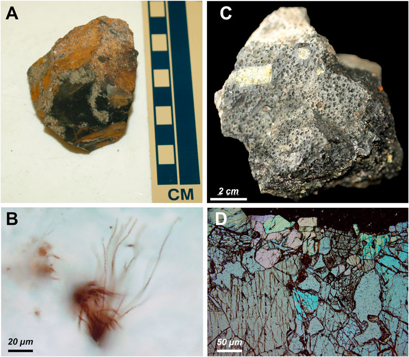
FIGURE 1. (A) Photograph of a hand sample of chert from the 1.9 billion years old Gunflint Formation, Canada, and (B) image in optical microscopy in transmitted light of the associated thin section permitting observation of microfossils otherwise impossible to see. (C) Basalt from Svalbard and (D) microscope observation of the associated thin section in cross-polarized transmitted light.

Raman Spectroscopy

Raman spectroscopy is a vibrational spectroscopy using a laser to identify and characterize atomic bonds. It is particularly suited for astrobiology since it permits the detection of both organic and inorganic biosignatures (e.g., kerogen, pigments, and bio-minerals, etc.) (Jehlicka et al., 2009; Marshall et al., 2010; Vandenabeele et al., 2012; Vitek et al., 2012; Bower et al., 2013; Edwards et al., 2013; Foucher and Westall, 2013; Campbell et al., 2015; Baqué et al., 2016; Jehlička et al., 2016; Foucher, 2019). In the laboratory, Raman spectroscopy is generally interfaced with an optical microscope permitting localisation of areas of interest and to carry out analyses at the micrometre scale. On the other hand, remote Raman and/or field systems, including the NASA Mars 2020 SHERLOC and SuperCam systems and the ESA/Roscosmos ExoMars 2022 Raman Laser Spectrometer, have a large spot size of several tens or hundreds of microns (Rull et al., 2017; Wiens et al., 2017). The spectra obtained correspond then to a mix of the spectra associated to the different components of the rock. This is particularly problematic when a phase is fluorescent because it generally masks the Raman signal of all the other phases. It has also been shown that the analysis of powdered samples can alter the spectroscopic signal (Foucher et al., 2013). Finally, the loss of texture associated with crushing means that Raman mapping cannot be used, despite the fact that they are particularly useful for the identification of microfossils (Foucher and Westall, 2013; Foucher et al., 2015; Bower et al., 2016, p. 16; Foucher, 2019). The development of a Raman micro-imager for planetary exploration is technically feasible since optical and scanning systems compatible with space environment already exist (Lopez-Reyes et al., 2013; Rull et al., 2017).

Laser Induced Breakdown Spectroscopy

This method uses a laser to create a plasma from the target sample and the emitted light is analysed by optical spectroscopy to determine its elemental composition. LIBS is already used on Mars during the NASA MSL and Mars 2020 missions with the ChemCam (Cousin et al., 2012; Grotzinger, 2013) and SuperCam (Wiens et al., 2017) instruments, respectively. In the laboratory, LIBS can be interfaced with optical microscopes to make analysis at the micrometre scale and to carry out elemental imaging (Fabre et al., 2018). It has also been shown that this method can be used to make isotopic dating by analysing specific minerals (Devismes et al., 2016). The possibility to make thin sections during planetary exploration would permit such analysis in situ.

Cathodoluminescence

This method uses an electron beam to induce the luminescence of a material. It is used in geosciences to detect trace elements and to understand the formation processes of minerals and rocks (e.g., Rusk et al., 2008). It has been shown to be relevant and compatible with space exploration (Thomas et al., 2009; Bost et al., 2013).

Fluid inclusion analysis

Fluid inclusions are small bubbles of gases or liquids trapped in minerals during their formation. Their analysis gives information on the environmental conditions (T, P, gases and liquids composition, salinity, etc.) existing when the rock formed. Such data would be particularly relevant to document the habitability of Mars by the past (Hode et al., 2003). Some inclusions on Earth also contain microbial remains and/or well preserved organic molecules (Mißbach et al., 2021) and are, therefore, particularly interesting for astrobiology.

Ice Analysis

Thin sections are commonly used to study the crystallinity of ices on Earth (e.g., Montagnat et al., 2010). Such observations would be relevant during the exploration of Mars as well as of the Jupiter’s and Saturn’s icy satellites.

Standard Protocol for Thin Section Preparation

The standard and inescapable steps for making a thin section are as follows:

1- A piece of rock is taken from the hand sample and indurated in epoxy resin, preferentially under vacuum in order to facilitate the penetration of the resin. Marks are made in order to maintain the orientation of the sample.

2- A slab is cut from the indurated piece of rock in order to have at least one flat surface.

3- The flat surface of the slab is glued onto a frosted glass slide generally using the same resin as previously used for induration.

4- The glued slab is cut parallel to the glass slide in order to keep a 50–200 µm thick slice of rock glued onto the glass slide.

5- The slice of rock is thinned down to 30–35 µm by grinding. This step permits control of the parallelism of the two faces of the slice.

6- The thin section is lapped to a final thickness of 30 µm and its surface is polished.

The cutting steps can be done using a circular diamond saw or a wire saw. The grinding is carried out using circular grinder and the polishing is made with abrasive discs of various grain sizes. These cutting, grinding and polishing steps are generally made using water in order to remove the dust, facilitate the mechanical cutting and grinding, and to cool the material and the sample. The induration phase is crucial since it gives competency to the sample and prevents cracking or breaking during the different steps.

Thin Section Preparation Device for Space Exploration

Due to its high relevance, a thin section preparation device was envisioned relatively early in the history of space exploration. Thus, in the 1965, even if it was not used, a semi-automated system to be used by the astronauts named Petralab was developed for the Apollo Applications Program and Advanced Lunar Programs at USGS, Flagstaff, by Paul Cary from the NASA Astrogeology department (Dreyer et al., 2013b).

Since the Apollo missions, all the other exploration missions of extraterrestrial bodies were robotic. The preparation of thin section should thus be envisioned in a fully-automated way and not necessarily using standard environmental conditions. However, the pressure and temperature at the surface of extraterrestrial bodies in the solar system are not compatible with the use of liquid water and may compromise the use of resins. Considering these difficulties, a fully-automated preparation of simply polished sections (which does not permit observation in transmitted light) was envisioned by ESA in the framework of the Multi-User Facility for Exobiology Research project (Battistelli, 2000). In this study, the starting sample was a drill core that was successively ground and polished in order to facilitate the optical (reflected light), Atomic Force Microscopy (AFM) and Raman spectroscopy observations, prior to being crushed for APXS and Mössbauer analyses. Also, in the pre-project of the ExoMars mission, the Sample Preparation Subsystem was initially able to polish the drill cores and to incorporate powdered rocks into resin for Mössbauer analyses (Schulte, 2000). While it was demonstrated that cutting and polishing were feasible, the scientific interest of the observations in reflected light was considered too low and the system was finally abandoned. Research on the induration phase was not undertaken for similar reasons.

Recently, Dreyer et al. (2013a), Dreyer et al. (2013b) proposed and tested a prototype of automated thin section preparation device for space exploration called IS-ARTS for in situ Automated Rock Thin Section Instrument (Paulsen et al., 2013). This system permits making thin sections from centimetric samples of any shape. The sample is handled using an innovative system called “Rock Gripper” consisting of an array of spring loaded pins permitting adaptation to any sample shape. The sample is moved linearly and is successively cut, glued onto a glass slide, cut again and observed. The sample is cut using a wire saw and the sample is glued with wax. The induration of the sample is only envisioned for further developments. This promising system, thus, demonstrates the feasibility of making thin sections on extraterrestrial bodies.

More broadly, a compact all-in-one thin section preparation system is interesting for scientific field exploration on Earth. Goren (2014), for example, proposed a non-automated portable thin section preparation laboratory. Even though this system requires human intervention, it demonstrates the feasibility of making thin sections with a limited amount of material and using small batteries.

Here, we present the LithoSpace project, begun in 2012 and supported by the CNES since 2014 by their Research and Technology program, which adapts the standard laboratory thin section preparation protocol to automated planetary exploration. Based on a different approach, it proposes an alternative system to that envisioned by Dreyer et al. (2013a), Dreyer et al. (2013b) and by Goren (2014). The specifications of these devices are compared to those expected for the LithoSpace system in Table 1. The size, mass and average power were estimated based on the specifications of the ExoMars 2022 rover (analytical laboratory dimensions ∼ 140 × 130 × 50 cm, mass = 310 kg, maximum drill power 70 W). Among the differences with other systems, we propose to use a disc saw rather than a wire saw since, by experience, a disc saw is more reliable and the surface finish after cutting is generally better. The samples are also systematically indurated. For astrobiological purposes, the most interesting rocks to study are sedimentary rocks which may be particularly fragile and brittle except when indurated by a cement. Indeed, this is the situation of the sediments in Gale Crater on Mars. In order to validate these choices, we carried out energy consumption experiments and tested the feasibility of cutting indurated samples in the absence of liquid water. Finally, we propose a dimensionally optimized device making 30 µm thick thin sections from drill cores in a fully-automated way. While no functional prototype has been developed yet, several technical solutions are proposed and a model serving as a “proof-of-concept” was made based on the specifications of our system. Interestingly, we took the opportunity to use this project to make students aware of space exploration. Thus, fifth year students at the engineering school Polytech’ Orléans, University of Orléans, France, and students in BTS (2-year technical degree) course “Industrialisation of Mechanic Products” and in Licence Pro “Technical Coordinator of Industrialization Methods” from the Benjamin Franklin high school of Orléans, France, participated in the development of the system using Computer Aided Designed and in making a demonstration model.

TABLE 1

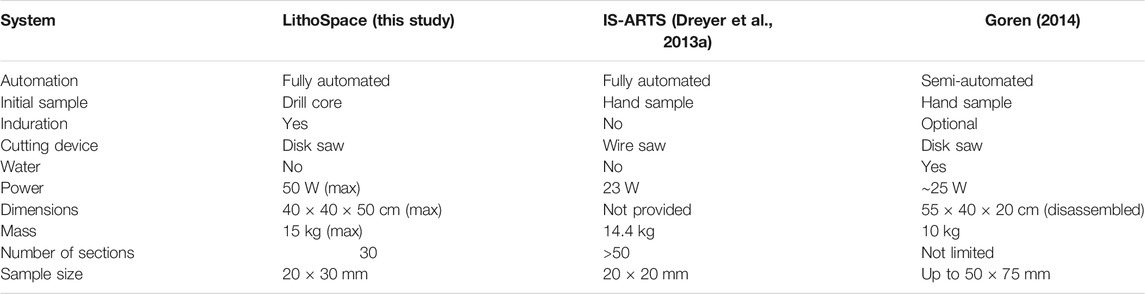
TABLE 1. Comparison between the envisioned LithoSpace system specifications with those proposed by Dreyer et al. (2013a) (IS-ARTS) and by (Goren, 2014).

Materials and Methods

Envisioned Protocol

We considered that thin sections will be prepared from 2.5 cm long and 1 cm diameter cylinders, similar to the ExoMars drill cores (Vago et al., 2017) and comparable in diameter to the drill cores taken by the Perseverance Mars 2020 rover (Farley et al., 2020). The envisioned protocol is described in Figure 2. We considered that the cores are pushed out of the drill into a sample receiving drawer that emerges from the interior of the rover, similar to the Core Sample Transport Mechanism (CSTM) of the Sample Preparation and Distribution System (SPDS) of the ExoMars mission (Vago et al., 2017). Photographs of the drill cores are made using the cameras located outside the rover. In our study, these images would be used to know the sample orientation. The drawer is then moved back into the rover. During the ExoMars mission the collected drill core is subsequently crushed while in our study it could be placed in an induration tank.

FIGURE 2

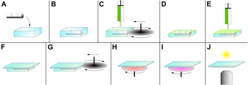
FIGURE 2. Schematic protocol for automated thin section preparation. (A–C) A drill core is placed into a container and indurated. (C,D) The whole is cut in the middle along the core axis. (E,F) A layer of resin is deposited and a glass slide is glued on the top of the remaining sample. (G) The sample is cut close to the glass slide in order to keep a ∼100 µm thick slice of rock. (H,I) The rock surface is ground and polished. (J) The 30 µm rock thin section is analysed from the bottom with an inverted microscope.

In order to validate the feasibility of this protocol in the absence of water, cutting tests were undertaken using different types of rock. The power required to cut the rocks and their final surface finish were studied.

Rock Samples

The proposed protocol was tested using a series of rocks of various compositions and physical properties. Most of these samples come from the International Space Analogue Rockstore (ISAR), http://isar.crns-orleans.fr, (Bost et al., 2013).

Basalt. Basalt from the Massif Central was chosen for its high relevance for Mars (ISAR reference 14FR08).

Komatiite. Komatiites are very primitive ultramafic rocks considered as good analogue for Mars (Bost et al., 2015). The sample comes from South Africa (ISAR reference 10ZA09).

Chert. The 3.45 billion year old Kitty’s Gap chert from the Pilbara, Australia, (ISAR reference 00AU05) was chosen for its analogy with putative fossiliferous Martian rock (Bost et al., 2015; Vago et al., 2017; Westall et al., 2006; Westall et al., 2011; Westall et al., 2013; Westall et al., 2015). It was also chosen because it is considered as one of the hardest rocks on Earth (7 on the Mohs scale of mineral hardness).

Chalk. Chalk was chosen for its very low hardness and for its tendency to form sticky powder/paste during sawing and grinding.

The samples were cut into 1 cm thick slabs and indurated into standard epoxy resin (Araldite^®) prior the tests.

Sample Preparation Instruments

Two disc saws were used at CEMHTI, CNRS, Orléans, France, for cutting tests.

Disc saw Presi P100 This simple system uses a variable speed electric engine to drive the disc. The sample is fixed on the top of the saw and the applied force is set using different weights. The cutting is thus carried out at constant load. For the tests, an ESCIL NC100 disc, 100 mm diameter, 0.3 mm thick was used and small brushes were added at the bottom of the saw to remove dust in the absence of water.

Disc saw Struers Secotom-10 This precise cutting device is equipped with two variable speed electric engines, one to drive the disc and one to move the sample. Contrary to the Presi P100 device, cutting is made at constant sample displacement speed. The load, i.e., the force applied by the sample onto the saw, was measured during the cutting. Tests were carried out using an ESCIL R100-5 disc, 100 mm diameter, 0.4 mm thick and small brushes were added at the bottom of the saw to remove dust from the disc in the absence of water.

These systems were plugged into a power meter in order to evaluate their power consumption. It is important to note that this power corresponds to the maximal power used, not to the power really delivered by the engines, since the power meter does not take into account the phase shift existing between the intensity and the voltage associated with AC engines and since a part of the power is used for the electronics.

Analysis Devices

All the analyses were made at CBM, CNRS, and Orléans.

Optical microscopy observations were carried out using an Olympus BX 51 microscope, both in transmitted and reflected light.

Surface roughness was estimated by Atomic Force Microscopy (AFM) using a Veeco Dimension 3,100 system in contact mode (Budget Sensors Cont-Al tips). The surface of the samples was scanned perpendicularly to the cutting streaks. Data processing was made using the WSxM software (Horcas et al., 2007).

Raman spectroscopy was used to characterize the sample. All the experiments were carried out using a WITec Alpha 500RA system equipped with a green laser (Nd:YAG frequency doubled laser) of wavelength λ = 532 nm. Raman imaging, obtained by 2D scanning of the sample surface, was used to document the mineralogy. For this study, a × 20 Nikon E Plan (numerical aperture N.A. = 0.40) objective was used. Raman spectra were acquired using a 600 g/mm grating spectrometer ranging from approximately −150 to 3,800 cm⁻¹ and a resolution ranging from 3 to 5 cm⁻¹. Laser power at the sample surface was set to 13 mW. Detailed information on micro-Raman imaging can be found in Foucher et al. (2017).

Results

Power Consumption

Presi P100 Disc saw

The power consumption of the system with the engine off is 6 W. At maximum disc rotation speed, the system consumes 46 W (i.e., without sample). The return to zero is not associated with a return to standby consumption but with a basic consumption of ∼20 W due to the phase shift not taken into account by the power meter.

The first cutting test was performed on the chalk sample. For practical reasons related to the sample fixation system, cutting was carried out parallel to the longitudinal axis of the chalk (see Figure 3). For the load, a mass of 185.5 g was chosen for the test, more or less arbitrarily. Figure 3 shows the evolution of electricity consumption over time.

FIGURE 3

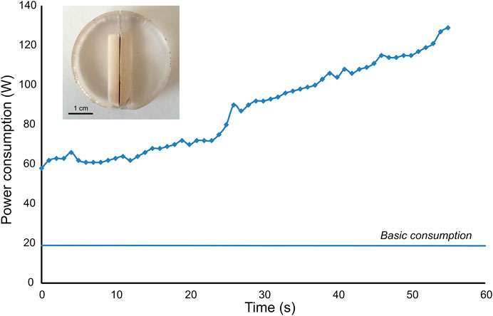
FIGURE 3. Evolution of power consumption over time during the cutting of a chalk sample (in insert) using the Presi P100 disc saw.

It is shown that the power consumption increases slowly during the first 15 min and then increases regularly over time to reach 129 W after 55 min. Cutting was then stopped because the machine became very hot. Thus, part of the increase in consumption can be attributed to Joule heating. After a break of 30 min, cutting resumed but was stopped immediately because the blade broke. By this time more than 80% of the sample had been cut.

Struers Secotom-10 Disc saw

The power consumption of the system with all engines off is 10 W. When cutting, it is impossible to stop the water pump which consumes 35 W. With the electronics, the system therefore consumes 45 W with the engines off. Switching on followed by a return to zero did not make any difference in power consumption on this system. The variation in consumption of the motor allowing the movement of the sample varies little with the sample displacement speed v_s. The difference in consumption between the maximum (v_s = 3 mm s⁻¹) and minimum (v_s = 0.005 mm s⁻¹) speed is only 5 W. In order to determine the power consumption of the system with respect to the disc rotation speed v_d, tests were carried out without a sample with a speed v_s = 0.005 mm s⁻¹. In the studied range (300–1,500 rpm), the power consumption P increases linearly with the speed of rotation of the disc according to the equation p = 0.025 v_d + 119.71 (see Figure 4A). The system allows samples to be cut through the section so the blade only cuts 1 cm of sample at the same time.

FIGURE 4

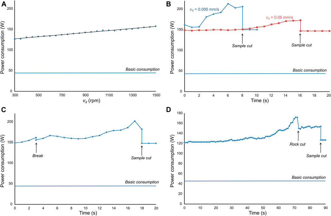
FIGURE 4. (A) Power consumption of the Struers Secotom 10 disc saw versus disc rotation speed. (B–D) Power consumption versus time for various samples and parameters: (B) chert sample, water on, v_d = 900 rpm and v_s = 0.095 mm s⁻¹ (in blue), and v_d = 900 rpm and v_s = 0.05 mm s⁻¹ (in red), (C) komatiite sample, water off, v_d = 900 rpm and v_s = 0.05 mm s⁻¹, (D) basalt sample, water off, v_d = 300 rpm and v_s = 0.01 mm s⁻¹.

Chert Sample

A first chert sample was cut with water using a disc rotation speed v_d = 900 rpm and a sample displacement speed v_s = 0.095 mm s⁻¹. The consumption before cutting was 150 W. Figure 4B shows the changes in power consumption over time. The cutting time was 8 min. It was observed that the electrical consumption increases rapidly with a peak at 213 W. This increase in consumption results in a significant increase of the load on the control panel. Once the sample was cut, the consumption fell back to its initial value (i.e. 150 W). A second sample was cut with a sample displacement speed that was twice as low v_s = 0.05 mm s⁻¹. The consumption before cutting was 147 W. The cutting time of the sample was logically double, i.e., 16 min (see Figure 4B). Nevertheless, it was shown that the power consumption increases slowly and reaches a maximum of 173 W at the very end of the cutting. The increase of the load on the control panel remains small. Once the sample was cut, the consumption fell back to its initial value (i.e., 147 W).

Komatiite Sample

The komatiite sample was cut without using water with a disc rotation speed v_d = 900 rpm and a sample displacement speed v_s = 0.05 mm s⁻¹. The consumption before cutting was 148 W. Figure 4C shows the changes in power consumption over time. In order to check disc heating, the system was stopped after 3 min; there was only a relatively limited increase in temperature. After this check, the blade was slightly retracted before resuming cutting. It then took 2 min before cutting actually resumed. The cutting test finally lasted 18 min (3 min + 2 min +13 min) including 16 min of actual cutting. The load increase on the control panel remained small throughout cutting. The electricity consumption increased gradually and reached its maximum of 202 W at the end of cutting. Once the sample was cut, the consumption fell back to its initial value (i.e., 148 W).

Basalt Sample

The basalt sample was cut without water. The system was set with the slowest possible disc rotation speed, v_d = 300 rpm, and a sample displacement speed v_s = 0.01 mm s⁻¹. Figure 4D shows the changes in power consumption over time. The consumption before cutting was 122 W. Cutting the sample took 87 min. The load increase on the control panel remained small throughout cutting. The power consumption gradually increased and reached a maximum of 172 W after 72 min. A plateau was then observed at about 152 W from the 72nd minute and at the end of the cut. This corresponds to a part of the sample only composed of resin. Finally, once the sample had been completely cut, power consumption was slightly higher, 127 versus 122 W. This difference is attributable to the friction of the disc on the remaining sample surface.

Alteration of the Discs

NC100 Disc

When cutting the chalk sample, temperature checks (felt by touch) were performed after 5, 15 and 55 min. The disc-sample assembly temperature was cold, cold, and warm, respectively.

Cutting the resin was not a problem. It neither burned nor fouled the disc. The dry cleaning system of the disc allowed relatively good elimination of chalk on the disc despite the strong adhesion of the latter, as shown in the photograph of the disc at the end of the test (Figure 5A).

FIGURE 5

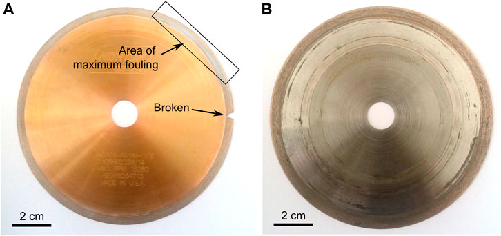
FIGURE 5. Discs after cutting tests. (A) NC100 disc used to cut the chalk with the Presi P100 disc saw. (B) R100-5 disc used to cut the chert, the komatiite and the basalt with the Struers Secotom-10 disc saw.

As previously stated, the test had to be stopped before the sample could be cut completely due to the break in the disc (see Figure 5A). This break is explained by the non-perfect perpendicularity of the disc with respect to the rotation axis. When cutting was resumed after the break, the disc saw had been restarted with the disc in the sample when, in fact, the sample should have been lifted and then placed back onto the rotating blade to take into account this defect of alignment. This lack of perpendicularity also explains the non-homogeneous fouling of the blade visible in Figure 5A. This break is only due the bad alignment of the Pressi P100 disc saw. Normally, these kinds of discs can cut several hundreds of rocks without breaking. Such a failure is not expected with the LithoSpace system and was thus not considered in the following.

R100-5 Disc

During dry cutting, both the sample and the disc warmed up. The longer the cutting time, the higher the temperature. In the case of the basalt sample, this resulted in the start of carbonization of the resin as well as of the bristles of the brushes used to remove the dust from the disc (Figure 5B). As these polymeric materials become sticky with heat, the blade cleaning system was less efficient. The disc and the brushes were therefore relatively dirty at the end of cutting, as shown in Figure 5B.

Surface State

Chalk Sample

Despite the fact that the disc was not perpendicular to the rotation axis, the cut surface of the chalk sample is relatively clean as shown in Figure 6.

FIGURE 6

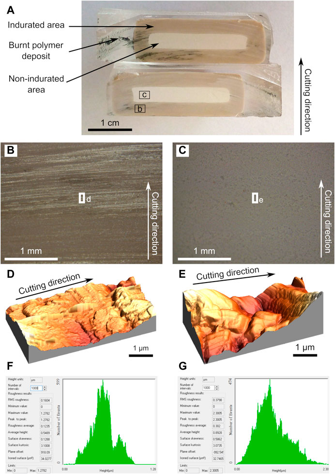
FIGURE 6. Chalk sample after cutting test on Presi P100 disc saw. (A) Image of the cut surface. (B,C) Optical microscopy images in reflected light of the areas indicated in (A). (D,E) AFM images of the areas indicated in (C,D) respectively and (F,G) associated roughness measurement.

In order to study the surface finish, the cutting of the sample was finished using a hacksaw, taking care not to touch the surfaces of the part already cut. A dark halo is observed in the sample (see Figure 6A). This corresponds to the zone of penetration of the resin during induration. The black areas observed are related to burnt polymer from the melting of the bristles of the cleaning system (Figure 6A). In reflected light optical microscopy, the cut streaks are more visible in the indurated zone than in the non-indurated zone (Figures 6B,C). However, AFM analyses show that the average roughness is lower in the indurated zone, 0.1235 µm against 0.302 µm in the non-indurated zone (Figures 6D–G). Due to the technical limitations of the AFM used, it was not possible to perform roughness analyses at a larger scale. These values are therefore largely underestimated. An estimate of the average roughness at the sample scale can be deduced from the maximum height measured on the AFM images. This gives a roughness of the order of 1.3 µm in the indurated zone and of 2.3 µm in the non-indurated zone (Figures 6F,G).

Chert Samples

Figure 7 shows the surface of the samples after cutting.

FIGURE 7

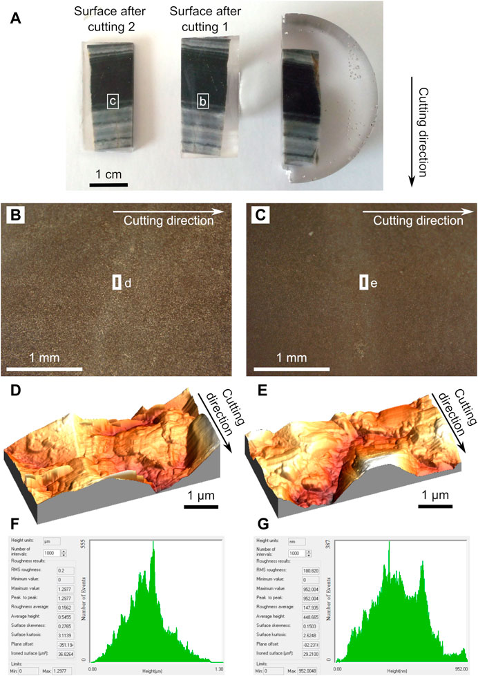
FIGURE 7. Chert samples after cutting with the Struers Secotom-10 disc saw. (A) Photograph of the three pieces of sample. (B,C) Optical microscopy images in reflected light of the areas indicated in (A). (D,E) AFM images of the areas indicated in (B,C) respectively and (F,G) associated roughness measurement.

The photograph (Figure 7A) shows that the surface finish is particularly homogeneous under the two cutting conditions (1-fast and 2-slow). Very few cutting streaks are observed. In reflected light optical microscopy, the roughness appears to be slightly lower with the slower cutting speed (Figures 7B,C). AFM analyses confirm this difference in roughness, which is 0.156 μm for fast cutting against 0.015 μm for slow cutting (Figures 7D–G). The average roughness at sample scale is estimated to 1.3 µm for fast cutting and 0.95 µm for slow cutting (Figures 7F,G).

Basalt Sample

Figure 8 shows the surface of the samples after cutting.

FIGURE 8

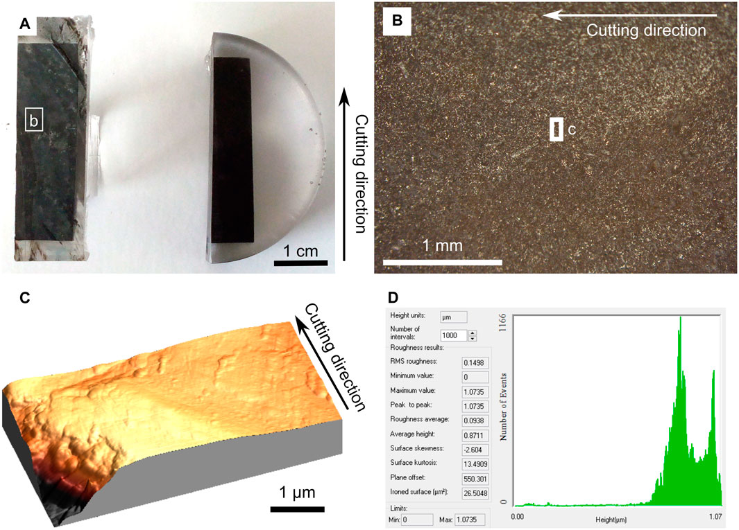
FIGURE 8. Basalt sample after cutting with the Struers Secotom-10 disc saw. (A) Photograph of the two parts of the sample. (B) Optical microscopy image in reflected light of the area indicated in (A). (C) AFM image of the areas indicated in (B,D) associated roughness measurement.

Cutting streaks are visible in the photograph (Figure 8A). In particular, black areas are observed associated with burnt polymer originating from the bristles of the cleaning system. In optical microscopy, the roughness appears to be low (Figure 8B). AFM analyses show a roughness of 0.094 µm (Figures 8C,D). The average roughness at sample scale is estimated to 1.1 µm (Figure 8D).

Komatiite Sample

Figure 9 shows the surface of the samples after cutting.

FIGURE 9

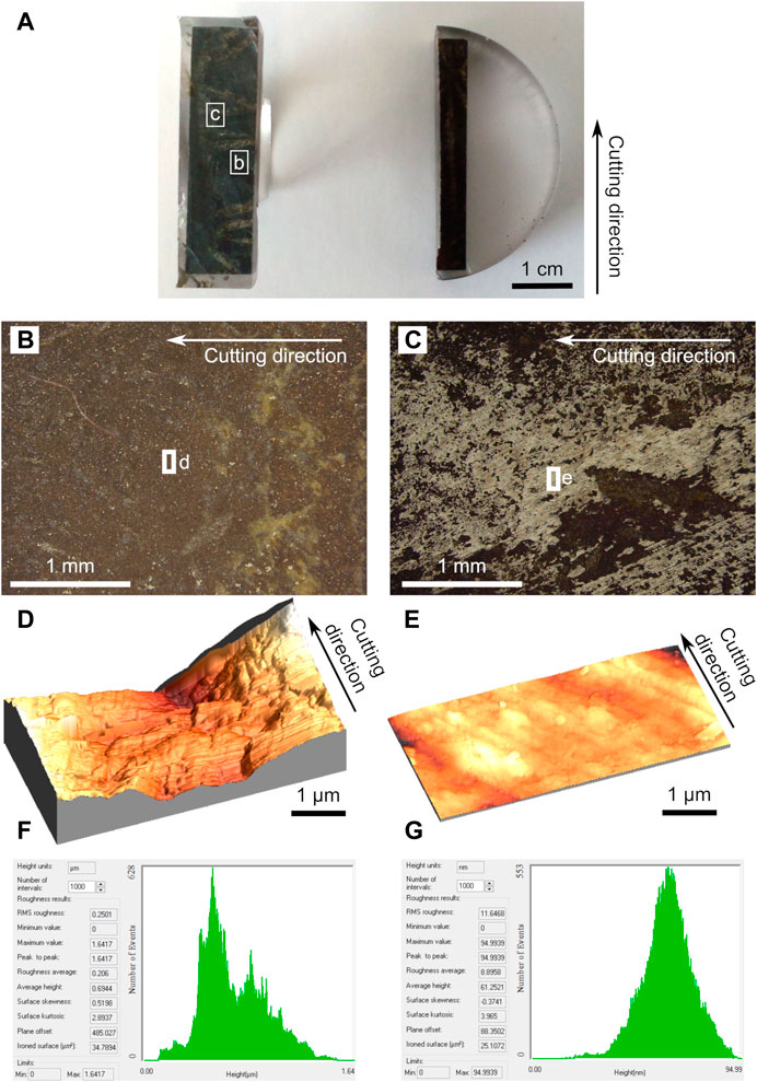
FIGURE 9. Komatiite sample after cutting with the Struers Secotom-10 disc saw. (A) Photograph of the two parts of the sample. (B,C) Optical microscopy images in reflected light of the areas indicated in (A). (D,E) AFM images of the areas indicated in (B,C) respectively and (F,G) associated roughness measurement.

The photograph (Figure 9A) shows that the surface finish is relatively homogeneous. Very few cutting streaks are observed. Visually, some areas appear more reflective than others. In reflected light optical microscopy, these two types of surface finish are clearly visible, with reflective areas appearing in light grey (Figure 9C). AFM analyses indicate a significant difference in roughness between the two types of surfaces: 0.206 µm for matt areas against 0.009 µm for shiny areas (Figures 9D–G). The average roughness at sample scale is estimated at 1.6 µm for the matt areas and 0.06 µm for the reflective areas (Figures 9F,G).

Raman Analysis

In order to detect the possible presence of contamination, analyses by Raman spectroscopy were carried out on the various zones studied in Section Surface state (see Figure 10).

FIGURE 10

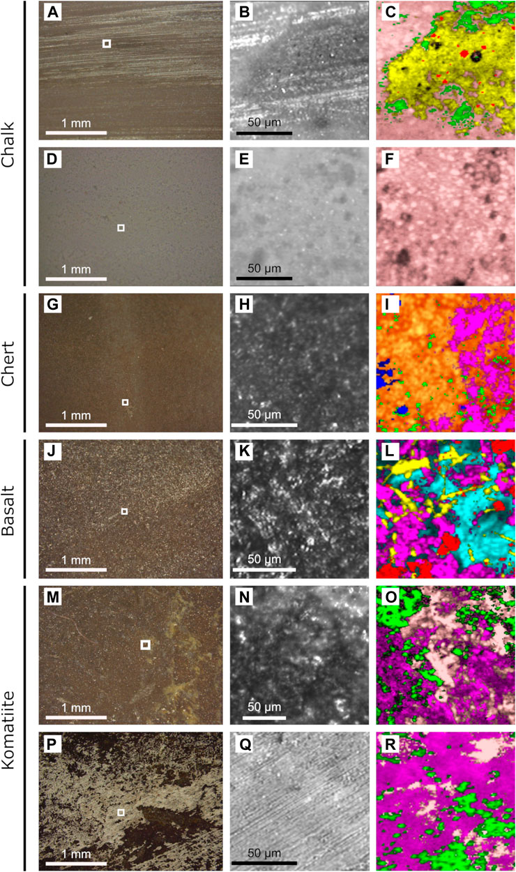
FIGURE 10. Raman analyses of the samples after cutting. For each sample, the analysed area is denoted by a small white square in the reflected light micrograph on the left. (A,B) reflected light optical microscopy images of the indurated area of the chalk sample. (C) Raman spectroscopy compositional map with calcite in pink, amorphous silica in yellow, carbonaceous material in green and an unidentified phase in red. (D,E) reflected light optical microscopy images of the non-indurated area of the chalk sample. (F) Raman spectroscopy compositional map showing only calcite in pink. (G,H) reflected light optical microscopy images of the chert sample (slow cut). (I) Raman spectroscopy compositional map with muscovite in fuchsia, anatase in dark blue, carbonaceous material in green, and quartz in orange. (J,K) reflected light optical microscopy images of the basalt sample. (L) Raman spectroscopy compositional map with augite in fuchsia, labradorite in light blue, hematite in red, and apatite in yellow. (M,N) reflected light optical microscopy images of a matt part of the komatiite sample. (O) Raman spectroscopy compositional map with talc in pink, antigorite (serpentine) in fuchsia, and carbonaceous material in green. (P,Q) reflected light optical microscopy images of a bright part of the komatiite sample. (R) Raman spectroscopy compositional map with talc in pink, antigorite (serpentine) in fuchsia, and carbonaceous material in green.

Raman analyses of chalk are in agreement with the expected composition, namely calcite with a trace of amorphous silica. Carbonaceous material potentially associated with burnt resin and/or burnt brush bristles is also detected. It is difficult to attribute the unidentified phase with contamination or not. Raman analyses of chert, basalt and komatiite are in agreement with the expected compositions. No contamination was detected. For the komatiite sample, the difference in surface finish between the matt and the reflective areas is not associated with difference in composition.

Discussion

Conclusions on Cutting Tests

Table 2 summarizes the various parameters and results associated with each cut. We define in particular:

1) The basic consumption, which is the consumption of the system powered on, all engines off. This consumption is linked to the design of the instrument (electronics, indicator lights, etc.). With a view to develop a space instrument, this can be greatly reduced.

2) The power without sample, which corresponds to the consumption of the system switched on before cutting the sample. This consumption is linked to the speed of the engines and to their design (quality of bearings, friction, loss by Joule heating, etc.). This consumption can therefore be greatly reduced too.

3) The maximum power, which corresponds to the maximum consumption of the system reached during cutting.

4) The useful power without sample, which is the consumption only attributable to the engines when they are running but without cutting. It corresponds to the power without sample minus the basic consumption.

5) The maximum useful power, which is the maximum consumption attributable to the engines during cutting. It corresponds to the maximum power reached minus the basic consumption.

6) The minimum power, which is the minimum power required to cut the sample. It corresponds to the maximum useful power minus the useful power without sample. This power corresponds to the minimum power required to cut the sample for given v_d and v_s speeds.

TABLE 2

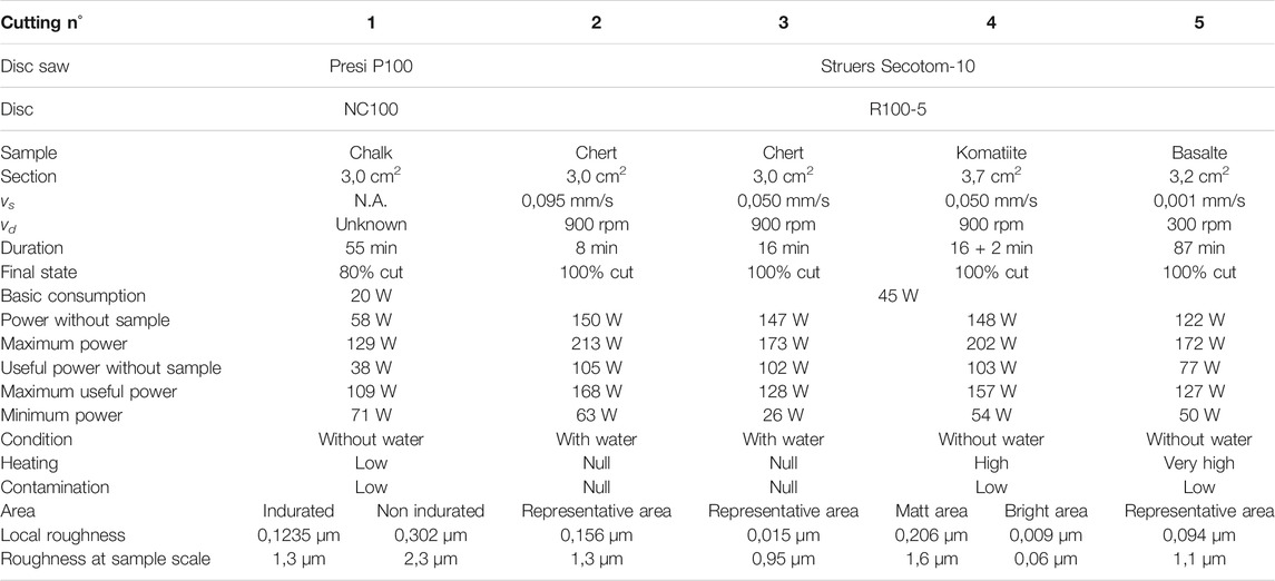
TABLE 2. Summary table of the various parameters and results associated with each cut (v_s: sample displacement speed; v_d: disc rotation speed).

The parameter that most influences the power required to cut a rock is the load, represented here by v_s. The greater the sample force on the disc, the more the system consumes power, as clearly shown by the two cuts made in the chert sample. It is thus preferable to cut with a constant load, as for the Pressi P100 saw, rather than with a constant sample displacement speed, as with the Struers Secotom-100 saw. Nevertheless, the load must be high enough to cut the rock in a reasonable time. A compromise must therefore be found between cutting time and load.

The absence of water has several consequences. First, the disc and sample could not cool down and the temperature increased. The greater the load, the greater the heating. Secondly, dust is not efficiently removed from the cut line and fouls the saw, which becomes less sharp. This increases the friction between the disc and the sample resulting in the increase of the temperature and of the load when working at constant sample displacement speed. Thus, despite identical cutting parameters, the power consumption is much greater during dry cutting of the komatiite sample than during the second cutting of the chert sample. Consequently, it is important to note that, in the absence of water, the hardness is not the relevant parameter to consider to evaluate the capacity of a system to cut a rock but rather its propensity to stick to the saw when cut. It would thus be potentially easier to cut a chert than a mudstone, for example.

The surface finish of the samples after cutting is related to roughness and contamination. Roughness depends on several factors. The nature of the sample plays an important role as evidenced by cutting tests performed on chalk and komatiite. Cutting tests carried out on chert show that a high load tends to increase the surface roughness. However, for all the tests, the “large” surface roughness remains very limited (less than 2 µm), meaning that the rock can be glued onto the glass slide directly after cutting as envisioned in the proposed protocol (cf. Figure 2), i.e., no lapping is required.

Contamination of the sample is related to the absence of water. The disc scrubbing system used did not efficiently remove cut-off residues, which remain attached to the brushes and induce contamination from one sample to another. The polymer bristles melted and then burned, partially contaminating the samples and the disc. This can be strongly improved by using, for example, a pumice jaw system that would remove dust from the blade during cutting. Nevertheless, cutting and grinding activities generate a lot of dust and it would be necessary to find a way to clean the tools between each use, as well as the thin sections before observation.

Finally, this study shows that it is possible to cut samples, including very hard rock, such as cherts, with a system whose power is less than 150 W. Moreover, it is important to note that the systems used for the tests are relatively large and are not as optimized as a space system would be.

Towards a Space System

The cutting tests demonstrated the feasibility of cutting a rock sample without water and with a relatively limited power. Most of the difficulties encountered can be circumvented by controlling the load applied to the sample and the temperature and by adding an efficient disc and sample cleaning system. We thus focussed the further investigations on the automation of the protocol described in section Envisioned protocol (see Figure 2). As displayed in Figure 11, we propose a system composed of three superimposed discs which can rotate independently from each other. The upper disc contains the glass slide distribution system and holder. The middle disc 2 has a notch to hold the induration tank and a brush to remove dust from the sample surface. Finally, the lower disc is composed of an empty section and 3 sections of various thicknesses permitting vertical displacement of the tank. Above these three discs are the sample arrival chute from which the drill cores arrive, the induration tank dispenser, the resin dispenser and the sawing area with a retractable disc saw located vertically between the discs 3 and 2. The bottom part of the system is composed of the microscope objective (or any other instrumental probe), the polishing disc, the grinding disc and the bin to store the cutting residues. By rotating the discs, it is possible to make and observe a thin section according to the different steps described in Figure 11. All along the preparation the orientation of the sample is known based on the images made outside the rover.

FIGURE 11

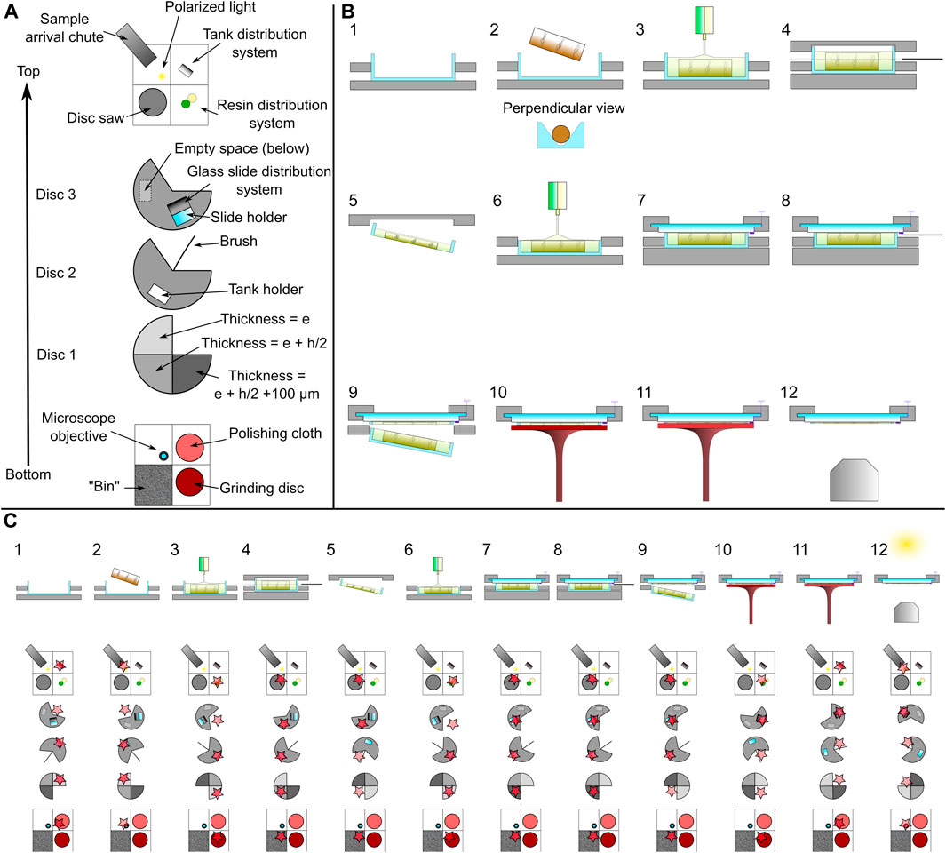
FIGURE 11. LithoSpace system. (A) The system is composed of three superimposed discs which can rotate independently of each other. The upper part of the system is composed of the sample arrival chute, from which the drill cores arrive, the induration tank dispenser, the resin dispenser, and the sawing area with a retractable disc saw. The upper disc (disc 3) is only 2/3 full. It contains the glass slide dispenser and holder. There is an empty mould on its underside to maintain the tank holder during sawing. Disc 2 is also 2/3 full. It has a notch to hold the induration tank and a brush to remove dust from the sample surface. The lower disc (disc 1) is composed of an empty section and 3 sections of various thicknesses permitting vertical displacement of the tank: e (typically e = 1 cm), e + h/2 with h the induration tank thickness (typically h = 1.5 cm), and e + h/2 + 100 µm. Finally, the bottom part of the system is composed of the microscope objective (or any other instrumental probe), the polishing disc, the grinding disc and the bin to store the cutting residues. (B) By moving the discs it is possible to make and observe a thin section in 12 steps as described in (C). 1- An induration tank is inserted from the tank distribution system in the dedicated hole in disc 2, onto the part of thickness e of disc 1. 2- The three discs rotate to place the tank below the arrival chute from which the drill cores fall. The tanks have a triangular profile in such a way that the cores necessarily fall in a centred position. 3- The three discs rotate to place the sample below the resin dispenser and the core is the covered with resin and indurated. 4- Disc 3 is positioned so that the hollow on its lower part is aligned with the tank then disc 1 is positioned on the part of thickness e + h/2 so as to bring up the tank which then becomes wedged in disc 3. Finally, the tank plus the drill core assembly is cut through its middle. 5- The assembly turns in order to come above the “bin” and discs 2 and 1 rotate in order to evacuate the upper part of the sample. 6- Disc 1 returns to its starting position of thickness e in order to lower the sample. The three discs rotate to place the sample below the resin dispenser where resin is deposited onto the cut surface of the sample. 7- A glass slide is slid into the slide holder. Disc 1 then raises the sample half the thickness of the tank plus 100 µm so that it is glued onto the glass slide (part of the disc of thickness e + h/2 + 100 µm). 8- The sample is cut again to a thickness of 100 µm relative to the surface of the glass slide. 9- The three discs rotate to the “bin” position and disc 3 is rotated on its empty part to evacuate the bottom part of the sample. 10- The section is ground in order to correct the parallelism of the faces and to reduce its thickness to ∼32 µm. The grinding stop is controlled by a circuit breaker. 11- The thin section is polished in order to decrease the roughness and to reach the final thickness of 30 µm. 12- The polished thin section is presented to the observation/analytical system(s). The position of the discs during the different steps are detailed in (C). The stars indicate the position of the sample.

System Improvement

In the absence of time constraints–the device is not yet designed for a specific mission–the opportunity was taken to use this project as a support for teaching. Thus, students in fifth year at the engineering school Polytech’, University of Orléans, and students in BTS (2-year technical degree) “Industrialization of Mechanical Products” and in professional license of “Technical Coordinator of Industrialization Methods” from the Benjamin Franklin high school of Orléans, worked on the optimisation of the system and on the development of a demonstration model. Different optimisations proposed are displayed in Figure 12.

FIGURE 12

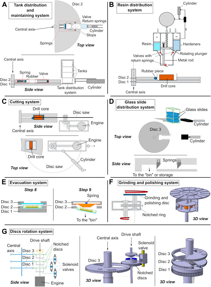
FIGURE 12. Possible LithoSpace system improvements. (A) Tank distribution and maintaining system. In this solution, the induration tanks are stored in a column located on the side of the discs in such a way that the bottom tank is aligned with disc 2. A cylinder is used to push the tank within the empty mould in disc 2 where it is maintained between a valve composed of two stops fixed with return springs and a rubber piece mounted on springs. (B) Resin distribution system. The solution proposed permits the mixing of the resin and its hardener. A cylinder is used to push the two components down into a tank where they are mixed using a metal rod fixed on a rotating plunger that turns and moves down. The system is designed in such a way that the correct quantity and ratio of resin/hardener is reached when the plunger reaches the valves of the resin and hardener tanks. The plunger is pushed down to its maximum to expel the mixed resin/hardener mixture onto the drill core in the induration tank. (C) Cutting system. In this system, the disk saw is driven using an engine and moved to the cutting position using a cylinder. The sawing of the sample is carried out by moving the sample on the disc saw by rotation of the 3 discs. (D) Glass slide distribution system. The glass slides are thinned on their edges so that they can be inserted into grooves and moved horizontally within the disc 3. They are pushed using a cylinder and maintained by two stops fixed on springs. When another slide is inserted, it pushes away the previous one which falls into the “bin” or another storage system. (E) Evacuation system. In order to remove the samples from disc 2, a moving section can be fixed below disc 3 with a spring to push the samples down. (F) Grinding and polishing system. In order to avoid polishing streaks on the surface of the thin sections it is proposed to used double axis rotation to create a loop movement. This method is commonly used in standard polishing or sanding devices. (G) Disc rotation system. Instead of rotating the disc from the central axis, it is proposed to induce the movement from their side. Each of the 3 discs is thus surrounded by a notched ring in contact with rotating, notched rings. The rotation of the notched rings is induced by a common drive shaft activated by a solenoid valve.

Tank Distribution and Maintaining System

The tanks are used to indurate the drill cores. One tank is required per sample. In the proposed system (Figure 12A) the tanks are stored vertically and a cylinder is used to insert one of them into disc 2. The tank is maintained in the disc using springs and valves. This solution offers the advantage of using only a single actuator.

Resin Distribution System

Consideration was given to a system allowing the mixing of a standard polyepoxy resin (Araldite 2020). This resin is compatible with vacuum and may harden at relatively low temperature (until 10°C), thus requiring low heating. UV hardening resins were not considered because they are not compatible with opaque rocks. Cyanoacrylate glues were not considered because their hardening requires liquid water (humidity). The system proposed in Figure 12B is composed of two compartments, one containing the epoxy resin and the other the hardener. Valves allow the application of the correct amount of resin and hardener in a chamber with a mixing rod. Cylinders allowing the application of the products from the side chambers are also present if the low gravity of the explored extraterrestrial body is not enough to permit a natural flow of the liquids. Finally, the central chamber consists of a cylinder for the application of the product. An engine rotates a mixing rod while at the same time pushing down the mixture onto the sample. This nice solution is however relatively complex to implement and it is probable that single-dose syringes would be preferred in the final version of the system.

Cutting System

There are two possibilities for the cutting phases: either they are carried out at constant sample displacement speed, or they are carried out at constant load. Nevertheless, previous experience has demonstrated that it better to work at a constant load in order to limit heating and also because of potential sample inhomogeneity. The chosen solution presented in Figure 12C consists of an engine rotating the disc saw and a cylinder pushing the disc saw onto the sample to be cut at a constant load.

Glass Slide Distribution System

The technical solution displayed in Figure 12D is very close to the tank distribution system described in Section Tank distribution and maintaining system. A cylinder is used to push the glass slide into the disc 3. The shape of the slides is designed in order to be slid into the thickness of the disc. Once a thin section has been analysed, it is pushed by the next one and falls into the bin or into a storage system.

Evacuation System

After the second cut (step 8), in order to obtain a 100 μm thick section, it is necessary to evacuate the bottom of the tank; however, this part of the sample is held in the cavity due to the springs present in the disc 2 (see Figure 12A). In order to facilitate its evacuation, a cone mounted onto a spring is added in the disc 3 as illustrated in Figure 12E. It permits pushing down of the bottom part for the tank into the bin as it passes underneath. An identical system is also in the disk 3 to evacuate the top part of the sample in step 5.

Grinding and Polishing System

In order to avoid creating scratches, grinding and polishing systems generally use a combination of at least two rotation motions (e.g., by rotating both the disc and the sample). In order to reproduce this double movement, the double axis rotation system shown in Figure 12F has been proposed. It can also be envisioned to use a disc having an outer abrasive area for grinding and an inner abrasive area for polishing as proposed by Dreyer et al., 2013b and Paulsen et al., 2013.

Disc Rotation System

The solution displayed in Figure 12G consists in notching the discs on their outer periphery. The discs are in contact with notched discs that can be connected to a rotating drive shaft using solenoid valves. When a solenoid valve is in the top position, a bevel gear comes into contact and transmits the motor torque to the notched disc which in turn drives the corresponding disc. This solution allows easy synchronization for steps requiring the rotation of several plates at the same time while allowing independent rotations with a single motor, in both directions of rotation. It therefore represents a saving in terms of weight and size compared to a solution requiring 3 separate engines.

Demonstration Model

As noted above, the project is still in progress and we are far from the development of a working system. Nevertheless, much progress has been made. In order to promote the project, it was thus decided to develop a demonstration model serving as a “proof-of-concept.” Thus, still in collaboration with the students from the Benjamin Franklin high school, a physical model in polycarbonate was made to be presented to the public as displayed in Figure 13. Samples, as they would be at the different steps, have also been prepared (see Figure 13C). It is planned to motorize this model in order to make it “functional” in the near future.

FIGURE 13

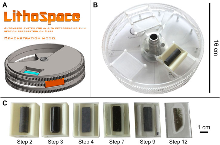
FIGURE 13. LithoSpace demonstration model. (A) 3D model. (B) Physical model. (C) Samples representative to the different preparation steps (see Figure 11).

Conclusion

The possibility to analyse petrographic thin sections in situ on extraterrestrial bodies would constitute an important advance in space exploration. In particular, it will permit structural and textural study of a rock, fine scale mineralogical analysis, and, with respect to Mars, detection of putative traces of fossilised microbial life. It would also open up the possibility of multiple techniques, from optical microscopy to micro-Raman and micro-LIBS imaging. With these advantages in mind, we proposed development of an automated thin sections maker for in situ space exploration in the framework of the LithoSpace project.

Among the difficulties considered were the absence of liquid water, the power consumption and the automation of the standard protocol. Using a series of tests, we demonstrated the feasibility of cutting rocks of various hardness and competency without water, and using power consumption compatible with space probe. We then proposed a system to carry out the automated protocol in a limited volume using three superimposed discs rotating independently to each other. Technical solutions were then proposed for the different steps by students from the Polytech’ engineering school and from the Benjamin Franklin high school. Finally, a demonstration model serving as a “proof-of-concept” to be presented during congresses has been made and was already shown at the 42nd COSPAR meeting in 2018 in Pasadena, United States, and during the European Planetary Science Congress 2018 in Berlin, Germany. The project was very well received by the scientific community, which was particularly enthusiastic about the possibility to analyse thin sections in situ.

Finally, even if the system has been initially though for automated space missions, it could be particularity useful for future human exploration. Indeed, its small bulk facilitates its incorporation within future extraterrestrial habitats. Similarly, the system could be relevant for the preparation of thin sections from the samples bring back to Earth during sample return missions by facilitating the preparation in sterile conditions. More broadly, a compact all-in-one thin section preparation system would be of interest for scientific field exploration on Earth, as demonstrated by the portable thin section preparation laboratory (non-automated) proposed before by Goren (2014).

Data Availability Statement

The authors confirm that the data supporting the findings of this study are available within the article. The raw data are available on request from the corresponding author, FF.

Author Contributions

FF supervised the project, conceptualized the protocol and the system, make the experiments and wrote the original draft. NB supervised the project, conceptualized the protocol and the system, make the experiments and review the original draft. SJ conceptualized the protocol and the system, make the experiments and review the original draft. AF supervised the students from Polytech’ engineering school, conceptualized the protocol and the system and review the original draft. NL review the original draft. PP, MB and FL supervised the students from the Benjamin Franklin high school, conceptualized the system and review the original draft. MV, PC, FC, and MV conceptualized the protocol and the system and review the original draft. FW supervised the project and reviewed and corrected the original draft.

Funding

The LithoSpace project is funded in the framework the CNES Research and Development programme.

Conflict of Interest

The authors declare that the research was conducted in the absence of any commercial or financial relationships that could be construed as a potential conflict of interest.

The handling editor declared a past collaboration with the authors FF and FW.

Publisher’s Note

All claims expressed in this article are solely those of the authors and do not necessarily represent those of their affiliated organizations, or those of the publisher, the editors and the reviewers. Any product that may be evaluated in this article, or claim that may be made by its manufacturer, is not guaranteed or endorsed by the publisher.

Acknowledgments

We thank the CNES for funding. We thank the CEMHTI laboratory for the use of the Presi P100 and Struers Secotom-10 systems. We thank the students for their contribution: Jianyu Li and Thomas Platel from Polytech’ Orléans, France, and Charles Fidanza, Laël Ibala, Clémence Navereau, Stanilas De Olivera, Nicolas Perricot, Romain Segret, Baptiste Smeets, Ulysse Tastet, Adrien Tessier-Neilel, Quentin Truchot, and Vincent Vaidie from the Benjamin Franklin high school, Orléans, France.

References

Baqué, M., Verseux, C., Böttger, U., Rabbow, E., de Vera, J.-P., and Billi, D. (2016). Preservation of Biomarkers from Cyanobacteria Mixed with Mars-Like Regolith under Simulated Martian Atmosphere and UV Flux. Orig Life Evol. Biosph. 46, 289–310. doi:10.1007/s11084-015-9467-9

PubMed Abstract | CrossRef Full Text | Google Scholar

Battistelli, E. (2000). Phase A Study for a Multi-User Facility for Exobiology Research (No. EXO-RP-GAL-001). Campi Bisenzio, Italy: European Space Agency, Galileo Officine.

Bost, N., Westall, F., Ramboz, C., Foucher, F., Pullan, D., Meunier, A., et al. (2013). Missions to Mars: Characterisation of Mars Analogue Rocks for the International Space Analogue Rockstore (ISAR). Planet. Space Sci. 82-83, 113–127. doi:10.1016/j.pss.2013.04.006

CrossRef Full Text | Google Scholar

Bost, N., Ramboz, C., LeBreton, N., Foucher, F., Lopez-Reyes, G., De Angelis, S., et al. (2015). Testing the Ability of the ExoMars 2018 Payload to Document Geological Context and Potential Habitability on Mars. Planet. Space Sci. 108, 87–97. doi:10.1016/j.pss.2015.01.006

CrossRef Full Text | Google Scholar

Bower, D. M., Steele, A., Fries, M. D., and Kater, L. (2013). Micro Raman Spectroscopy of Carbonaceous Material in Microfossils and Meteorites: Improving a Method for Life Detection. Astrobiology 13, 103–113. doi:10.1089/ast.2012.0865

PubMed Abstract | CrossRef Full Text | Google Scholar

Bower, D. M., Steele, A., Fries, M. D., Green, O. R., and Lindsay, J. F. (2016). Raman Imaging Spectroscopy of a Putative Microfossil from the ∼3.46 Ga Apex Chert: Insights from Quartz Grain Orientation. Astrobiology 16, 169–180. doi:10.1089/ast.2014.1207

PubMed Abstract | CrossRef Full Text | Google Scholar

Campbell, K. A., Lynne, B. Y., Handley, K. M., Jordan, S., Farmer, J. D., Guido, D. M., et al. (2015). Tracing Biosignature Preservation of Geothermally Silicified Microbial Textures into the Geological Record. Astrobiology 15, 858–882. doi:10.1089/ast.2015.1307

PubMed Abstract | CrossRef Full Text | Google Scholar

Cousin, A., Sautter, V., Fabre, C., Maurice, S., and Wiens, R. C. (2012). Textural and Modal Analyses of Picritic Basalts with ChemCam Laser-Induced Breakdown Spectroscopy. J. Geophys. Res. 117, E10002. doi:10.1029/2012je004132

CrossRef Full Text | Google Scholar

Devismes, D., Gillot, P.-Y., Lefèvre, J.-C., Boukari, C., Rocard, F., and Chiavassa, F. (2016). KArMars: A Breadboard Model forIn SituAbsolute Geochronology Based on the K-Ar Method Using UV-Laser-Induced Breakdown Spectroscopy and Quadrupole Mass Spectrometry. Geostand Geoanal Res. 40, 517–532. doi:10.1111/ggr.12118

CrossRef Full Text | Google Scholar

Dreyer, C. B., Schwendeman, J. R., Steele, J. P. H., Carrell, T. E., Niedringhaus, A., and Skok, J. (2013a). Development of a Thin Section Device for Space Exploration: Rock Cutting Mechanism. Adv. Space Res. 51, 1674–1691. doi:10.1016/j.asr.2012.12.013

CrossRef Full Text | Google Scholar

Dreyer, C. B., Zacny, K., Steele, J. P. H., Schwendeman, J. R., Paulsen, G., Andersen, R. C., et al. (2013b). Development of a Thin Section Device for Space Exploration: Overview and System Performance Estimates. Adv. Space Res. 51, 1659–1673. doi:10.1016/j.asr.2012.12.012

CrossRef Full Text | Google Scholar

Edwards, H. G. M., Hutchinson, I. B., Ingley, R., Parnell, J., Vítek, P., and Jehlička, J. (2013). Raman Spectroscopic Analysis of Geological and Biogeological Specimens of Relevance to the ExoMars Mission. Astrobiology 13, 543–549. doi:10.1089/ast.2012.0872

PubMed Abstract | CrossRef Full Text | Google Scholar

Fabre, C., Devismes, D., Moncayo, S., Pelascini, F., Trichard, F., Lecomte, A., et al. (2018). Elemental Imaging by Laser-Induced Breakdown Spectroscopy for the Geological Characterization of Minerals. J. Anal. Spectrom. 33, 1345–1353. doi:10.1039/C8JA00048D

CrossRef Full Text | Google Scholar

Farley, K. A., Williford, K. H., Stack, K. M., Bhartia, R., Chen, A., de la Torre, M., et al. (2020). Mars 2020 Mission Overview. Space Sci. Rev. 216, 142. doi:10.1007/s11214-020-00762-y

CrossRef Full Text | Google Scholar

Foucher, F., and Westall, F. (2013). Raman Imaging of Metastable Opal in Carbonaceous Microfossils of the 700-800 Ma Old Draken Formation. Astrobiology 13, 57–67. doi:10.1089/ast.2012.0889

PubMed Abstract | CrossRef Full Text | Google Scholar

Foucher, F., Lopez-Reyes, G., Bost, N., Rull-Perez, F., Rüßmann, P., Westall, F., et al. (2013). Effect of Grain Size Distribution on Raman Analyses and the Consequences for In Situ Planetary Missions. J. Raman Spectrosc. 44, 916–925. doi:10.1002/jrs.4307

CrossRef Full Text | Google Scholar

Foucher, F., Ammar, M.-R., and Westall, F. (2015). Revealing the Biotic Origin of Silicified Precambrian Carbonaceous Microstructures Using Raman Spectroscopic Mapping, a Potential Method for the Detection of Microfossils on Mars. J. Raman Spectrosc. 46, 873–879. doi:10.1002/jrs.4687

CrossRef Full Text | Google Scholar

Foucher, F., Guimbretière, G., Bost, N., and Westall, F. (2017). “Petrographical and Mineralogical Applications of Raman Mapping,“ in Raman Spectroscopy and Applications. Editor K. Maaz (London: IntechOpen), 163–180. doi:10.5772/65112

CrossRef Full Text | Google Scholar

Foucher, F. (2019). “Detection of Biosignatures Using Raman Spectroscopy,” in Biosignatures for Astrobiology, Advances in Astrobiology and Biogeophysics. Editors B. Cavalazzi, and F. Westall (Cham: Springer International Publishing), 267–282. doi:10.1007/978-3-319-96175-0_13

CrossRef Full Text | Google Scholar

Goren, Y. (2014). The Operation of a Portable Petrographic Thin-Section Laboratory for Field Studies. N. Y. Microsc. Soc. Newsl. 1–17. September.

Google Scholar

Grotzinger, J. P., Crisp, J., Vasavada, A. R., Anderson, R. C., Baker, C. J., Barry, R., et al. (2012). Mars Science Laboratory Mission and Science Investigation. Space Sci. Rev. 170, 5–56. doi:10.1007/978-1-4614-6339-9_3

CrossRef Full Text | Google Scholar

Grotzinger, J. P. (2013). Analysis of Surface Materials by the Curiosity Mars Rover. Science 341, 1475. doi:10.1126/science.1244258

PubMed Abstract | CrossRef Full Text | Google Scholar

Hode, T., von Dalwigk, I., and Broman, C. (2003). A Hydrothermal System Associated with the Siljan Impact Structure, Sweden-Implications for the Search for Fossil Life on Mars. Astrobiology 3, 271–289. doi:10.1089/153110703769016370

PubMed Abstract | CrossRef Full Text | Google Scholar

Horcas, I., Fernández, R., Gómez-Rodríguez, J. M., Colchero, J., Gómez-Herrero, J., and Baro, A. M. (2007). WSXM: A Software for Scanning Probe Microscopy and a Tool for Nanotechnology. Rev. Sci. Instrum. 78 (1-8), 013705. doi:10.1063/1.2432410

PubMed Abstract | CrossRef Full Text | Google Scholar

Jehlička, J., Culka, A., and Nedbalová, L. (2016). Colonization of Snow by Microorganisms as Revealed Using Miniature Raman Spectrometers-Possibilities for Detecting Carotenoids of Psychrophiles on Mars?. Astrobiology 16, 913–924. doi:10.1089/ast.2016.1487

PubMed Abstract | CrossRef Full Text | Google Scholar

Jehlicka, J., Edwards, H. G. M., and Vitek, P. (2009). Assessment of Raman Spectroscopy as a Tool for the Non-destructive Identification of Organic Minerals and Biomolecules for Mars Studies. Planet. Space Sci. 57, 606–613.

Google Scholar

Lopez-Reyes, G., Rull, F., Venegas, G., Westall, F., Foucher, F., Bost, N., et al. (2013). Analysis of the Scientific Capabilities of the ExoMars Raman Laser Spectrometer Instrument. Eur. J. Mineral. 25, 721–733. doi:10.1127/0935-1221/2013/0025-2317

CrossRef Full Text | Google Scholar

Marshall, C. P., Edwards, H. G. M., and Jehlicka, J. (2010). Understanding the Application of Raman Spectroscopy to the Detection of Traces of Life. Astrobiology 10, 229–243. doi:10.1089/ast.2009.0344

PubMed Abstract | CrossRef Full Text | Google Scholar

Michel-Lévy, A., and Lacroix, A. (1888). Les minéraux des roches. Paris: Librairie Polytechnique Baudry et cie.

Mißbach, H., Duda, J.-P., van den Kerkhof, A. M., Lüders, V., Pack, A., Reitner, J., et al. (2021). Ingredients for Microbial Life Preserved in 3.5 Billion-Year-Old Fluid Inclusions. Nat. Commun. 12, 1101. doi:10.1038/s41467-021-21323-z

PubMed Abstract | CrossRef Full Text | Google Scholar

Montagnat, M., Weiss, J., Cinquin-Lapierre, B., Labory, P. A., Moreau, L., Damilano, F., et al. (2010). Waterfall Ice: Formation, Structure and Evolution. J. Glaciol. 56, 225–234. doi:10.3189/002214310791968412

CrossRef Full Text | Google Scholar

Paulsen, G., Zacny, K., Dreyer, C. B., Szucs, A., Szczesiak, M., Santoro, C., et al. (2013). Robotic Instrument for Grinding Rocks into Thin Sections (GRITS). Adv. Space Res. 51, 2181–2193. doi:10.1016/j.asr.2013.01.001

CrossRef Full Text | Google Scholar

Rull, F., Maurice, S., Hutchinson, I., Moral, A., Perez, C., Diaz, C., et al. (2017). The Raman Laser Spectrometer for the ExoMars Rover Mission to Mars. Astrobiology 17, 627–654. doi:10.1089/ast.2016.1567

CrossRef Full Text | Google Scholar

Rusk, B. G., Lowers, H. A., and Reed, M. H. (2008). Trace Elements in Hydrothermal Quartz: Relationships to Cathodoluminescent Textures and Insights into Vein Formation. Geol 36, 547–550. doi:10.1130/G24580A.1

CrossRef Full Text | Google Scholar

Schulte, W. (2000). Multi-User Facility for Exobiology Research. Munich, Germany: European Space Agency, Kayser-Threde.

Squyres, S. W., Arvidson, R. E., Bell, J. F, Brückner, J., Cabrol, N. A., Calvin, W., et al. (2004). The Spirit Rover's Athena Science Investigation at Gusev Crater, Mars. Science 305, 794–799. doi:10.1126/science.1100194

PubMed Abstract | CrossRef Full Text | Google Scholar

Thomas, R., Barbin, V., Ramboz, C., Thirkell, L., Gille, P., Leveille, R., et al. (2009). “Cathodoluminescence Instrumentation for Analysis of Martian Sediments,” in Cathodoluminescence and its Application in the Planetary Sciences. Editor A. Gucsik (Berlin, Heidelberg: Springer Berlin Heidelberg), 111–126. doi:10.1007/978-3-540-87529-1_6

CrossRef Full Text | Google Scholar

Thomson, B. J., Hurowitz, J. A., Baker, L. L., Bridges, N. T., Lennon, A. M., Paulsen, G., et al. (2014). The Effects of Weathering on the Strength and Chemistry of Columbia River Basalts and Their Implications for Mars Exploration Rover Rock Abrasion Tool (RAT) Results. Earth Planet. Sci. Lett. 400, 130–144. doi:10.1016/j.epsl.2014.05.012

CrossRef Full Text | Google Scholar

Vago, J. L., Westall, F., Landing, S., Coates, A. J., Jaumann, R., et al. Pasteur Instrument Teams (2017). Habitability on Early Mars and the Search for Biosignatures with the ExoMars Rover. Astrobiology 17, 471–510. doi:10.1089/ast.2016.1533

PubMed Abstract | CrossRef Full Text | Google Scholar

Vandenabeele, P., Jehlička, J., Vítek, P., and Edwards, H. G. M. (2012). On the Definition of Raman Spectroscopic Detection Limits for the Analysis of Biomarkers in Solid Matrices. Planet. Space Sci. 62, 48–54. doi:10.1016/j.pss.2011.12.006

CrossRef Full Text | Google Scholar

Vítek, P., Jehlička, J., Edwards, H. G. M., Hutchinson, I., Ascaso, C., and Wierzchos, J. (2012). The Miniaturized Raman System and Detection of Traces of Life in Halite from the Atacama Desert: Some Considerations for the Search for Life Signatures on Mars. Astrobiology 12, 1095–1099. doi:10.1089/ast.2012.0879

PubMed Abstract | CrossRef Full Text | Google Scholar

Westall, F., de Vries, S. T., Nijman, W., Rouchon, V., Orberger, B., Pearson, V., et al. (2006). The 3.466 Ga “Kitty’s Gap Chert”, an Early Archean Microbial Ecosystem. Geol. Soc. Am. Spec. Paper 405, 105–131. doi:10.1130/2006.2405(07)

CrossRef Full Text | Google Scholar

Westall, F., Foucher, F., Cavalazzi, B., de Vries, S. T., Nijman, W., Pearson, V., et al. (2011). Volcaniclastic Habitats for Early Life on Earth and Mars: A Case Study from ∼3.5Ga-old Rocks from the Pilbara, Australia. Planet. Space Sci. 59, 1093–1106. doi:10.1016/j.pss.2010.09.006

CrossRef Full Text | Google Scholar

Westall, F., Loizeau, D., Foucher, F., Bost, N., Betrand, M., Vago, J., et al. (2013). Habitability on Mars from a Microbial Point of View. Astrobiology 13, 887–897. doi:10.1089/ast.2013.1000

PubMed Abstract | CrossRef Full Text | Google Scholar

Westall, F., Foucher, F., Bost, N., Bertrand, M., Loizeau, D., Vago, J. L., et al. (2015). Biosignatures on Mars: What, Where, and How? Implications for the Search for Martian Life. Astrobiology 15, 998–1029. doi:10.1089/ast.2015.1374

PubMed Abstract | CrossRef Full Text | Google Scholar

Wiens, R. C., Maurice, S., and Rull-Perez, F. (2017). The SuperCam Remote Sensing Instrument Suite for the Mars 2020 Rover: A Preview. Spectroscopy 32 (5), 50–55.

Google Scholar