Impact of Foreshock Transients on the Flank Magnetopause and Magnetosphere and the Ionosphere

Introduction

Perturbations in front of the bow shock are more frequently observed in front of the quasi-parallel shock (the foreshock) and the perturbed region extends further upstream, as compared to those in front of the quasi-perpendicular shock. In this paper, the mesoscale perturbations generated in the foreshock are referred to as ion foreshock transients. There are many different types of foreshock transients with their time scales ranging from seconds to minutes and spatial scales ranging from foreshock ion gyroradius up to 10 R_E (Zhang and Zong, 2020). Almost all foreshock transient perturbations include a core with the number density and magnetic field strength lower than the background solar wind values and compression edge(s) with the density and magnetic field strength higher than the solar wind values. Some foreshock transients may also include flow deflection. Some foreshock transients are generated by the kinetic interaction of energetic ions reflected from the bow shock with interplanetary magnetic field (IMF) discontinuities, such as foreshock bubbles (Omidi et al., 2010; Turner et al., 2013; Liu et al., 2015, 2016; Omidi et al., 2020; Turner et al., 2020), hot flow anomalies (Chu et al., 2017; Lin, 1997, 2002; Liu et al., 2017; Lucek et al., 2004; Omidi and Sibeck, 2007; Schwartz et al., 1985; Schwartz et al., 2018; Thomsen et al., 1986; Zhang et al., 2010; 2017), foreshock cavities (e.g., Sibeck et al., 2002, 2004; Schwartz et al., 2006; Billingham et al., 2008), and traveling foreshock (e.g., Kajdičet al., 2017), while some are formed without IMF discontinuities, such as diamagnetic cavities (Lin, 2003; Lin and Wang, 2005), foreshock cavitons (Omidi, 2007; Blanco-Cano et al., 2011; Kajdičet al., 2013), and spontaneous hot flow anomalies (Omidi et al., 2013; Zhang et al., 2013). The foreshock transients that do not have the density core are foreshock compressional boundary (e.g., Sibeck et al., 2008) and short large-amplitude magnetic structures (e.g., Schwartz, 1991). Some of the above transients, such as HFAs, can also be generated in front the quasi-perpendicular shock. Recent MHD simulations found that the bow shock response to transient density depleted regions in the solar wind can also result in structures that resemble HFAs (Otto and Zhang, 2021).

The density perturbations of foreshock transients result in perturbations in dynamic pressure. As the perturbations propagate into the magnetosheath, they can cause magnetopause distortion. The resulting magnetosheath perturbations and the impact on the dayside magnetopause have been simulated (e.g., Lin and Wang, 2005; Omidi et al., 2016; Sibeck et al., 2021)) and observed (e.g., Archer et al., 2014; 2015; Jacobsen et al., 2009; Kajdičet al., 2021; Sibeck et al., 1999; 2000). Similar to the impact of the solar wind dynamic pressure perturbations, the magnetopause distortion driven by foreshock transients can subsequently generate ultralow frequency (ULF) waves inside the magnetosphere (e.g., Hartinger et al., 2013; Wang et al., 2017; Wang et al., 2018b; Wang et al., 2019; Wang B. et al., 2020; Shi et al., 2021; Wang B. et al., 2021), enhance particle precipitation and the resulting aurora brightness (e.g., Fillingim et al., 2011; Wang et al., 2018a; Wang et al., 2018b; Wang et al., 2019), and enhance field-aligned currents (FACs) and the associated perturbations in ionospheric currents and ground magnetic field (e.g., Kataoka et al., 2002; Murr and Hughes, 2003; Fillingim et al., 2011; Shen et al., 2018).

Recent studies have extended our understanding of the foreshock transients to the nightside. In observations, Liu et al. (2020; 2021) reported foreshock transients observed in the midtail foreshock around X ∼ –40 R_E. Using multi-point satellite measurements, Wang et al. (2018) showed that the perturbations driven by foreshock transients can propagate tailward within the flank magnetosheath to the midtail around X ∼ −50 R_E and can cause transient flank magnetopause distortion. 3D global hybrid simulations have been conducted to investigate foreshock transients associated with an IMF directional rotational discontinuity (RD) (Wang C. P. et al., 2020) and tangential discontinuity (TD) (Wang C. P. et al., 2021). They showed the evolution of the foreshock transient perturbations as they propagate from the dayside to nightside foreshock and the associated magnetosheath perturbations in the flanks. In this paper, we use the simulation by Wang B. et al. (2021) to show qualitatively the 3D structure of the flank magnetopause distortion caused by foreshock transients and the impact on the magnetosphere and ionosphere. The results presented here should provide a qualitative understanding of the impacts common to the foreshock transients of different types since they all have the same features of density perturbations (low-density core and high-density edge). We also present two observation events to provide qualitative comparisons with the simulated magnetopause distortion and ionospheric perturbations.

Simulation

Wang B. et al. (2021) used the AuburN Global hybrId CodE in 3D (ANGIE3D) hybrid code (Lin et al., 2014) to simulate foreshock transients resulting from the interaction of an IMF directional TD (i.e., with direction change only) with the foreshock ions. The simulation model and setup for this simulation is described in Simulation Model and Setup. In Magnetosheath Perturbations and Tailward Propagation, Dayside Magnetopause Distortion, Dayside Magnetopause Distortion, Flank Magnetopause Distortion, Impact on the Magnetosphere, Impact on the Ionosphere, we present the simulation results for the tailward propagating magnetosheath perturbations, the magnetopause distortion on the dayside and the flank, and the impacts on the magnetosphere and the ionosphere.

Simulation Model and Setup

In the ANGIE3D code, the ions (protons) are treated as discrete, fully kinetic particles, and the electrons are treated as a massless fluid. Quasi charge neutrality is assumed. Detailed descriptions of the equations for ion particle motion, electric and magnetic fields and assumptions used in the ANGIE3D code are given in Lin et al. (2014). The code is valid for low-frequency physics with ω ∼Ω_i and kρ_i ∼1 (wavelength λ ∼6ρ_i), where ω is the wave frequency, k is the wave number, Ω_i is the ion gyrofrequency, and ρ_i is the ion Larmor radius.

The simulation domain is 25 ≥ X ≥ −60, 60 ≥ Y ≥ −35, 35 ≥ Z ≥ −45 R_E in the geocentric solar magnetospheric (GSM) coordinates. Inflow time-dependent boundary conditions for the solar wind are specified at the sunward boundary and open boundary conditions are used for the rest of the outer boundaries. An inner boundary is assumed at the geocentric distance of r ≈ 3 R_E. This inner boundary is composed of a zigzag grid line approximating the spherical surface as in global MHD simulations. For the region of the inner magnetosphere, a cold, incompressible ion fluid is assumed to be dominant in r <6 R_E, which coexists with particle ions, since this simulation focuses on the dynamics and ion kinetic physics in the outer magnetosphere. The inclusion of the cold ion fluid in the inner magnetosphere simplifies the conditions for the fluid-dominant low-altitude, inner boundary. A combination of spherical and Cartesian coordinates is used at the inner boundary. We let particles be reflected at exactly r = 3 R_E. This simple reflection of the ion parallel velocity means that loss cone effects are omitted. The E and B fields at the boundary reside on the Cartesian boundary approximating the spherical boundary, which are extrapolated to an extra grid point inside the r = 3 R_E surface. The B field is assumed to maintain the dipole field values at the inner boundary.

The ionospheric conditions (1,000 km altitude) are incorporated into the ANGIE3d code. The FACs, calculated within the inner boundary, are mapped along the geomagnetic field lines into the ionosphere as input to compute ionospheric potential. For this simulation, simplified ionospheric conductance with uniform Pederson conductance of 10 siemens and Hall conductance of 5 siemens is specified.

The TD is specified as a planar IMF discontinuity with a half-width of 0.12 R_E and the normal direction of (−0.5, 0.86, 0). The TD propagates with a velocity of (−400, 0, 33.7) km/s. At t = 0, the TD plane intersects the Y = 0 axis at X = 185 R_E. Unless otherwise noted, downstream (upstream) of the TD in this paper indicates the anti-sunward (sunward) side of the TD. The downstream IMF direction is (3, 1.7, 0) nT and upstream IMF is (0, 0, −3.4) nT. Constant solar wind density of 5 cm⁻³ and isotropic solar wind ion temperature of 10 eV are used. The solar wind velocities are (−370.7, 16.8, 33.7) km/s downstream and (−400, 0, 0) km/s upstream. The average solar wind Alfvén Mach number is M_A = 11.8. These solar wind values are within the typically observed ranges. To accomplish this large-scale simulation with the available computing resources and can still produce physical results, we choose the solar wind d_i to be 0.1 R_E (about 6 times larger than the realistic value) and the cell dimensions to be n_x × n_y × n_z = 502 × 507 × 400. Also, we use time-independent nonuniform cell sizes (ranging from ∼0.1 to 0.5 R_E) so that we can appropriately assign cell sizes comparable to the d_i values in different key regions from the solar wind to the outer magnetosphere. The bow shock and magnetopause form self-consistently by the interaction of the solar wind with the geomagnetic dipole. Before the arrival of the TD, the bow shock nose is at X ∼14 R_E and the magnetopause nose is at X ∼10 R_E, similar to the realistic locations.

Magnetosheath Perturbations and Tailward Propagation

Figures 1A–C show the 2D profiles of the magnetic field strength (|B|), ion density (N), and ion bulk flow speed (|V|), respectively, in the X-Y plane at Z = 0 at four different times from t = 53.4–75.3 min (see also Supplementary Movie S1 in Supplementary Material). The simulated magnetopause and bow shock are disturbed, so we also add in the t = 53.4 min plots two smooth model boundaries, the magnetopause locations predicted by Roelof and Sibeck (1993) and the bow shock locations predicted by Peredo et al. (1995), as visual references to help readers discern the magnetosheath perturbations. In this stimulation, before the arrival of the TD, the foreshock is mainly on the duskside extending from the dayside to the nightside. Note that there are weak perturbations in the foreshock and the magnetosheath due to the foreshock ULF waves. The TD first encounters the foreshock ions just outside the dayside bow shock at t ∼44 min and foreshock transient perturbations are formed (see Wang B. et al. (2021) for more details about the initiation of the foreshock transient). The foreshock transient perturbations consist of a core with lower density, higher temperature, lower magnetic field strength, and lower anti-sunward bulk flow speed than the values of the solar wind. An edge with relatively higher density and higher magnetic field strength is on the upstream side of the core. As the TD (indicated by the black or white dashed straight lines) propagates tailward, it continues to interact with the foreshock ions and generate perturbations around the TD (the low-density core is indicted by magenta arrows in Figure 1B). The perturbations newly generated just outside the bow shock subsequently enter the magnetosheath via their anti-sunward flows and continue to propagate anti-sunward. Note that these magnetosheath perturbations associated with the foreshock transients are the focus of this paper, not the pre-existing perturbations associated with the foreshock ULF waves.

FIGURE 1

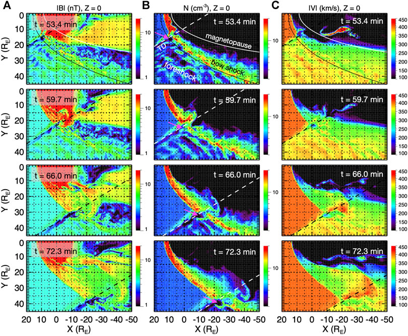
FIGURE 1. Time sequences of the X-Y distributions from t = 53.4–72.3 min at Z = 0 for (A) magnetic field strength, (B) number density, and (C) ion bulk flow speed. The straight white or black dashed lines indicate the projection of the TD plane. The white curve in the top panel indicates the model magnetopause from Roelof and Sibeck (1993) and the black curve indicates the model bow shock from Peredo et al. (1995). The magenta arrows in (B) indicate the low-density core.

Figure 1 shows the tailward propagation of the magnetosheath plasma and magnetic field perturbations resulting from foreshock transients. In the near-Earth region, as shown in the t = 53.4 and 59.7 min plots, the structures of magnetosheath perturbations are approximately aligned with the TD plane (the black or white dashed line). The perturbations seen closer to the magnetopause are associated with the foreshock transient perturbations that are generated and enter the magnetosheath earlier, while those seen closer to the bow shock are associated with the foreshock transient perturbations that are generated and enter the magnetosheath more recently. The newer perturbations coming into the magnetosheath interact nonlinearly with those further inside, leading to changes in the spatial structures of the perturbations across the magnetosheath. In this simulation, the foreshock region extends to the nightside. Thus, as the TD propagates from the near-Earth to the midtail, as shown in the t = 66 and 72.3 min plots, there are still new foreshock transient perturbations being continuously added into the flank magnetosheath. As a result, the magnetosheath perturbations are still strong in the midtail. Compared to the earlier magnetosheath perturbations in the near-Earth flank shown in the t = 59.7 min plots, which are more spatially confined around the TD plane and have well-defined structures, the spatial size of the mid-tail magnetosheath perturbations shown in the t = 72.3 min plots have become larger and their spatial structures become complex because of the nonlinear interaction described above.

Dayside Magnetopause Distortion

Figure 2 compares the dayside magnetosheath and magnetopause before the arrival of the TD at t = 45.6 min with those associated with the magnetosheath perturbations at t = 52.8 min. As shown in Figures 2A–E for the X-Y distributions at Z = 0, at t = 45.6 min, there are small and localized perturbations in both the magnetosheath plasma and the magnetopause shape (black or white curves) associated with the foreshock ULF waves. The dayside magnetopause locations are determined by tracing magnetic field lines from Z = 0 and the field lines in the dayside magnetosphere are closed (both ends of the field lines are in the ionosphere). At t = 52.8 min, the low-density core and high-density edge can be seen in the new perturbations forming outside the bow shock as well as in the magnetosheath perturbations that have entered the magnetosheath earlier (Figure 2B). The magnetic field strength is lower inside the core and higher at the edge (Figure 2A). Figure 2C shows different flow speeds and directions for the core and edge, which would later cause the spatial extents of the core and edge regions to change as they propagate tailward. As a result of the lower density and flow speed within the core than at the edge, both the thermal pressure (P_th) and the dynamic pressure along the direction normal to the magnetopause (P_dyn,n) (the magnetopause normal direction in this paper is estimated using the model magnetopause of Roelof and Sibeck (1993)) are relatively lower within the core and higher at the edge. As shown in Figure 2D, the dayside magnetopause and magnetosphere intrude locally outward for ∼3 R_E into the magnetosheath in response to the lower P_n (P_n = P_th + P_dyn,n) of the core and are distorted locally inward for ∼1 R_E by the stronger P_n of the edge. The outward intruding magnetosphere is indicated by the plasma with relatively higher magnetic field strength (Figure 2A) and lower density (Figure 2B) than the surrounding magnetosheath plasma. Figure 2E shows the perpendicular current density. It shows that the magnetosheath perturbations at t = 52.8 min results in strong perpendicular currents along the distorted magnetopause. Figures 2F,G show the 2D X(Y)-Z profiles along the white dashed line indicated in Figure 2A (the TD plane at t = 52.8 min). The magnetopause outward distortion is seen mainly in the region of |Z| < ∼ 5 R_E with the maximum distortion near Z = 0. The 1D profiles at Z = 0 along the white dashed line indicated in Figure 2A are shown in Figures 2H–K. Comparing the 1D profiles between t = 45.6 and 52.8 min clearly show the changes in magnetic field components, flow velocity components, and pressure components outside the magnetopause (vertical magenta dashed lines) associated with the low-density core.

FIGURE 2

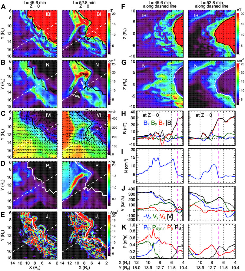
FIGURE 2. The X-Y distributions at Z = 0 for (A) magnetic field strength, (B) number density, (C) ion bulk flow speed and flow directions (black arrows), (D) pressure along the direction normal to the model magnetopause, (E) perpendicular current density at t = 45.6 (left panels) and 52.8 min (right panels). The straight white dashed lines indicate the projection of the TD plane at t = 52.8 min. The black or white curves in (A–G) indicate approximately the simulated magnetopause. The white dotted curves in (a) indicates the model magnetopause based on Roelof and Sibeck (1993). (F–K) The 2-D and 1-D profiles at t = 45.6 (left) and 52.8 min (right) along the TD plane at t = 52.8 min indicated in (a): The 2-D profiles for (F) magnetic field strength and (G) number density. The 1-D profiles at Z = 0 for (H) magnetic field components, (I) number density, (J) ion bulk flow velocities, and (K) pressures. The magenta dashed line in (H)–(K) indicate approximately the magnetopause.

Flank Magnetopause Distortion

Figure 3 compares the X-Y distributions of the nightside magnetosheath and magnetosphere at Z = 0 at t = 45.6 with those at t = 60 min when the magnetosheath perturbations have propagated to the nightside around X = –10 R_E. The magnetosheath perturbations at t = 60 min are seen to be around the TD line (white dashed line). Similar to the dayside magnetopause distortion shown in Figure 2, the magnetopause (indicated by white dashed line) intrudes locally outward into the magnetosheath around X = –10 R_E in response to the low-density core of the magnetosheath perturbations while it is distorted inward around X = –7 R_E in response to the high-density edge. In determining the nightside magnetopause boundaries shown in Figure 3 and later in Figures 4, 5, we investigate the magnetosonic Mach number from the magnetosheath to the magnetosphere and use the location of a quick drop in the Mach number values to below a certain threshold as the approximate location for the magnetopause boundary. The outward intruding magnetosphere can be seen by the plasma with relatively higher magnetic field strength (Figure 3A), lower density (Figure 3B), and higher temperature (Figure 3C) than the surrounding magnetosheath plasma. Different from the slow-flowing plasma deep within the magnetosphere, the intruding magnetospheric plasma has a strong tailward flow speed (Figure 3D). Figure 3E shows the changes in the perpendicular current density within the magnetosphere associated with the distorted magnetopause. This results in FACs flowing into and out of the ionosphere, as described later in Impact on the Ionosphere. Figure 3F shows the 3D view of the number density distributions at t = 60 min from three different viewing angles together with the magnetic field lines. As indicated by the closed magnetic field lines (red), the plasma sheet is seen within the outward intruding magnetosphere. The field lines in the magnetosheath tailward of the intruding magnetosphere are open field lines (purple, with one end connecting to the Earth) due to open flank magnetopause resulting from the duskward IMF downstream of the discontinuity, while those earthward of the intruding magnetosphere are IMF field lines (light pink) corresponding to the southward IMF upstream of the discontinuity.

FIGURE 3

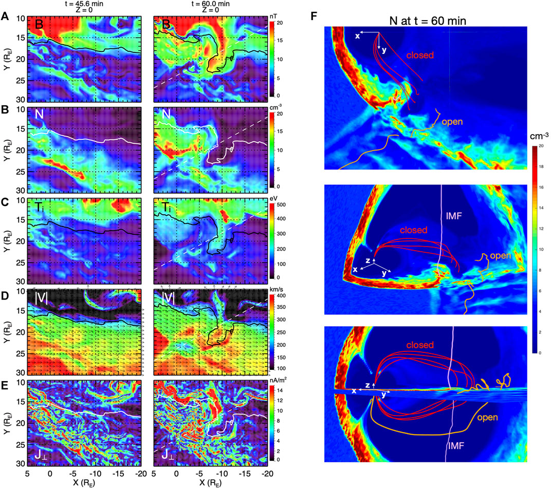
FIGURE 3. The X-Y distributions at Z = 0 for (A) magnetic field strength, (B) number density, (C) ion temperature, (D) ion bulk flow speed and flow directions (black arrows), and (E) perpendicular current density at t = 45.6 (left panels) and 60 min (right panels). The black or white curves indicate approximately the magnetopause boundary. The straight white dashed lines in the left panels indicate the projection of the TD plane at t = 60 min. (F) Number density distributions at t = 60 min viewing from three angles. The red curves indicate closed magnetic field lines, the orange lines indicate open magnetic field lines, and light pink lines indicate IMF field lines.

FIGURE 4

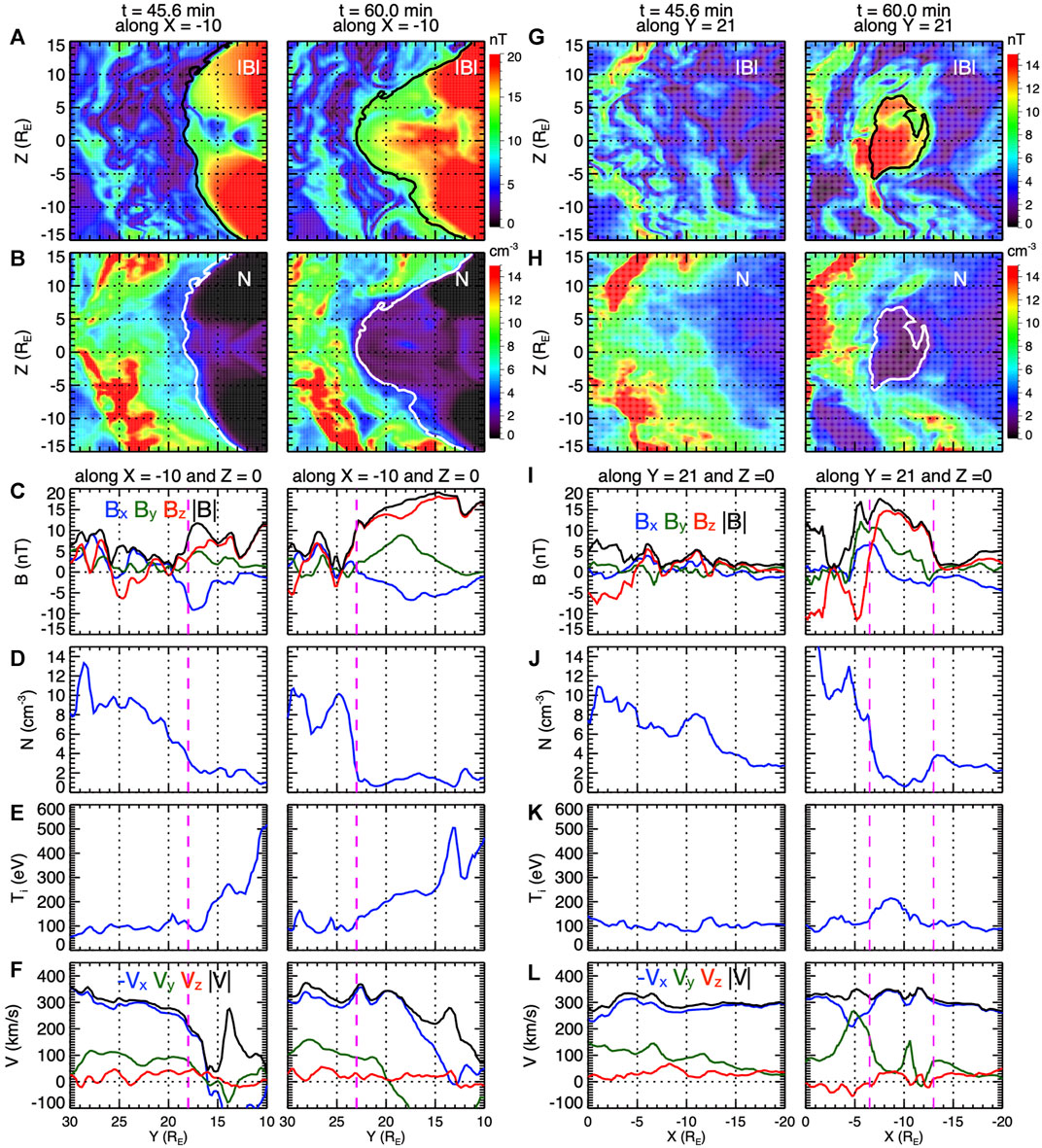
FIGURE 4. The Y-Z distributions at X = −10 R_E for (A) magnetic field strength and (B) number density and the Y profiles at X = −10 and Z = 0 R_E for (C) magnetic field components, (D) number density, (E) ion temperature, and (F) ion bulk flow velocities at t = 45.6 (left panels) and 60 min (right panels). The X-Z distributions at Y = 21 R_E for (G) magnetic field strength and (H) number density and the X profiles at Y = 21 and Z = 0 R_E for (I) magnetic field components, (J) number density, (K) ion temperature, and (M) ion bulk flow velocities at t = 45.6 (left panels) and 60 min (right panels). The white or black curves in (A–B) and (G–H) indicate approximately the magnetopause boundary. The vertical magenta dashed lines in (C–F) and (I–M) indicate the magnetopause.

FIGURE 5

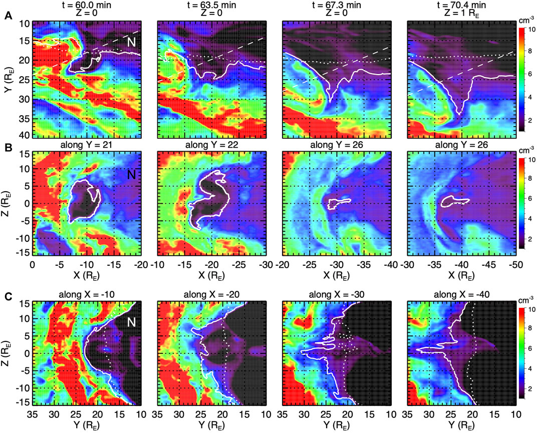
FIGURE 5. Time sequences of number density distributions in (A) X-Y, (B) X-Z, and (C) Y-Z planes from t = 60–70.4 min. The white solid curves indicate approximately the magnetopause. The white dotted curves in (A) and (C) indicate the magnetopause at t = 45.6 min. The straight white dashed lines in (A) indicate the projection of the TD plane.

The 3D structure of the outward intruding magnetosphere at t = 60 min shown in Figure 3 can be better constructed with the 2D Y-Z and X-Z distributions cutting through the intrusion shown in Figures 4A,B,G,H, respectively (see also Supplementary Movie S2 in Supplementary Material). The magnetopause is distorted mainly in the region from Z ∼ −10 to 10 R_E with the maximum outward distortion at Z ∼0 (Figures 4A,B) so that the cross-section in the X direction is the widest near Z = 0 (Figures 4G,H). The Y-profiles of plasma and magnetic field along the cutting plane at Z = 0 are shown in Figures 4C–F. As indicated by the vertical magenta dashed line, the magnetopause boundary moves outward from Y ∼18 to 24 R_E during the distortion. Figures 4I–M show the X-profiles at Z = 0 along Y = 21 R_E. The X scale of the intruding magnetosphere is ∼6 R_E.

Figures 5A–C show the time sequence of the flank magnetopause (white solid curves) distortion in the X-Y, X-Z, and Y-Z planes, respectively. The white dotted curves in Figures 5A,C indicate the magnetopause at t = 45.6 min. Note that the magnetopause boundary shape can appear filamentary at some locations. This is associated with fine structures of the magnetosheath perturbations in the magnetic field strength and flow speed, which resulting in fine structures in the magnetosonic Mach number distributions used in determining the approximate magnetopause boundary. Figure 5 shows that as the magnetosheath perturbations move tailward from X ∼ −10 to X ∼ −40 R_E, they continue to distort the magnetopause. As described in Magnetosheath Perturbations and Tailward Propagation, the spatial structures of magnetosheath perturbations change substantially as they propagate tailward, thus the 3D structure of the outward intruding magnetosphere in the midtail (t = 70.4 min plot) is quite different from the earlier structure in the near-Earth tail (t = 60 min plot). The maximum outward intrusion remains around Z = 0 and it extends farther out in the Y direction with increasing downtail distances. The localized structure of the outward distortion shown in Figure 5 indicates that a satellite in the magnetosheath may observe the outward intruding magnetosphere with the probability strongly depending on the satellite locations.

Figure 6 shows the temporal profiles of magnetic field components, number density, ion temperature, and ion bulk flow velocities that would be observed by a virtual satellite in the magnetosheath at three downtail distances at Z ∼0. Because of the passing of the localized outward magnetopause distortion, the virtual satellite would observe transient appearance of the magnetosphere, as indicated by the magnetic field strength, density, and temperature changing from the magnetosheath values to the magnetospheric values and then return to the magnetosheath values. These temporal profiles are qualitatively similar to the perturbations observed in the midtail magnetosheath at X = −54 R_E reported by Wang et al. (2018). Another observation event in the flank magnetosheath closer to the Earth is shown in An Event for Flank Magnetopause Distortion.

FIGURE 6

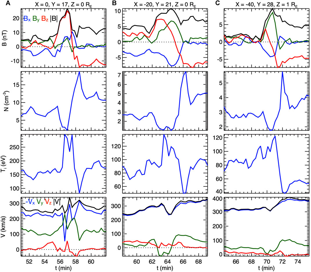
FIGURE 6. Temporal profiles at (A) X = 0, Y = 17, and Z = 0 R_E, (B) X = –20, Y = 22, and Z = 0 R_E, and (C) X = –40, Y = 28, and Z = 1 R_E. From top to bottom: Magnetic field components, number density, ion temperature, and ion bulk flow velocities.

Impact on the Magnetosphere

The localized and transient magnetopause distortion affects the magnetic field within the magnetosphere. Figure 7 shows a time sequence of the Y-Z distributions at X = −10 R_E from the dusk flank to midnight for number density (Figure 7A), magnetic field strength (Figure 7B), amplitudes of the magnetic field perturbations in the parallel direction (Figure 7C), and perpendicular current strength (Figure 7D). The magnetic field perturbations shown in Figure 7C are obtained by subtracting the 10 min running averages. To better show the perturbations associated with waves propagating through a relatively uniform background, only the perturbations in the northern lobe where B_x >15 nT are plotted in Figure 7C. As shown in the t = 45.6 min plot for before the arrival of the magnetopause distortion, there are weak magnetic field perturbations within the magnetosphere. These are due to the small magnetopause disturbances associated with the foreshock ULF waves, like that seen on the dayside as shown in Figure 2A for t = 45.6 min. As the magnetopause distortion passes through X = –10 R_E, as shown in the t = 59.7 – t = 61.6 min plots in Figure 7, the magnetic field perturbations within the magnetosphere are enhanced. The enhancements are seen to extend from the dusk flank into the magnetosphere. Compared to the enhancements when the magnetopause is distorting outward around t ∼60 min, the perturbations generated by the inward magnetopause distortion around t = 61.3 min are stronger and deeper into the magnetosphere. This shows that the magnetopause distortion driven by foreshock transients can launch compressional waves within the magnetosphere, which qualitatively explains the observed enhancements in magnetospheric ULF waves associated with foreshock transients (e.g., Hartinger et al., 2013; Wang et al., 2017; Wang et al., 2018b; Wang et al., 2019; Wang B. et al., 2020).

FIGURE 7

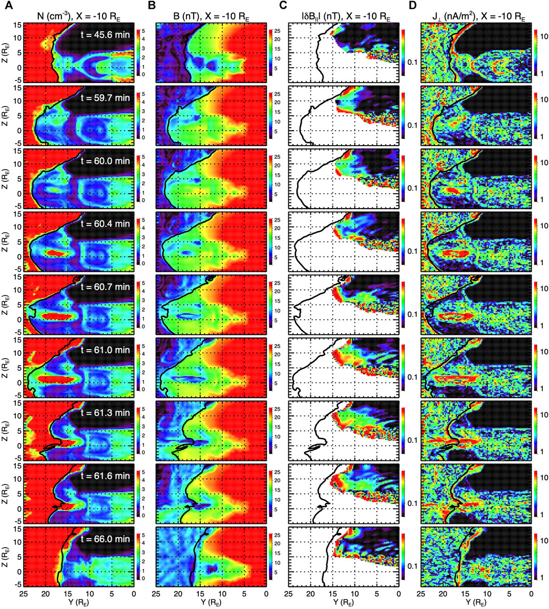
FIGURE 7. Time sequences of the Y-Z profiles at X = −10 R_E from t = 45.6–66 min for (A) number density, (B) magnetic field strength, and (C) the amplitudes of magnetic field perturbations in the parallel direction in the northern lobe where B_x >15 nT, and (D) perpendicular current density. The black curves indicate approximately the magnetopause.

As shown in Figure 7B, the inward and outward motion of the distorted magnetopause alters the magnetospheric magnetic field near the flank in Y >∼10 R_E. This causes transient changes in the perpendicular currents in the flank magnetosphere shown Figure 7D as well as FACs flowing into or out of the ionosphere in order to maintain current continuity, establishing impact on the ionosphere. The resulting FAC perturbations in the ionosphere are shown in Impact on the Ionosphere.

Impact on the Ionosphere

Figures 8A,B show the FACs and FAC perturbations at t = 60 min, respectively, in the Northern Hemisphere (N.H.) ionosphere (positive value indicates FACs flowing into the N.H. Ionosphere). The FAC perturbations are obtained by subtracting the 10 min averages of the FACs in the ionosphere. The FAC spatial distribution shown in Figure 8A has currents flowing into (out of) the ionosphere on the dawnside (duskside), which is the large-scale region-1 FACs connecting to the magnetosphere near the magnetopause. Figure 8B shows that the FAC perturbations are spatially localized. Figure 8C shows the time sequence of the ionospheric FAC perturbations in N.H. as a function of MLT and MLAT. Figure 8D shows the time series of N.H. FAC perturbations at different duskside MLT locations along MLAT = 73.5. Figures 8C,D show that the region of enhanced FAC perturbations moves anti-sunward from near noon toward later MLTs, which is consistent with the tailward propagation of the flank magnetopause distortion. At t = 60 min, FAC perturbations have moved to nightside at ∼18–20 MLT when the magnetopause distortion has propagated to nightside at X ∼ −10 R_E. The FAC perturbations would result in perturbations in the horizontal currents flowing in the ionosphere due to the current continuity, both would generate magnetic field perturbations on the ground.

FIGURE 8

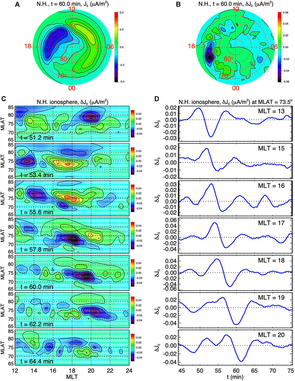
FIGURE 8. (A) FAC and (B) FAC perturbations at t = 60 min in N.H. (C) Time sequences of the MLAT-MLT distributions for the FAC perturbations in the ionosphere from t = 51.2–64.4 min (B) Time series of the FAC perturbations at different MLTs along MLAT = 73.5^o.

Note that simplified and spatially uniform ionospheric conductance is used in this simulation and we do not further evaluate the simulated ionospheric horizontal currents. The spatial distributions of the simulated ionospheric potential pattern and FACs corresponding to this uniform conductance do not have day-night and dawn-dusk asymmetries as realistic as those corresponding to non-uniform conductance that accounts for EUV and aurora contribution (Ridley et al., 2004). We expect that using realistic EUV- and aurora-generated conductance would shift the MLT and MLAT locations as well as the amplitudes of the perturbations in FAC and horizontal currents, but it would not affect their physical connection with the flank magnetopause distortion presented above. The simulated FAC perturbations seen at a fixed ionospheric location shown in Figure 8D should still provide a qualitative explanation for the observed ground magnetic field perturbations associated with foreshock transients (e.g., Shen et al., 2018). An observation event for ground magnetic field perturbations propagating to the nightside is shown in An Event for the Ionospheric Disturbances.

Observation Events

In this section, we present two observation events associated with foreshock transients for qualitative comparisons with the simulated flank magnetopause distortion and ionospheric perturbations presented in Simulation. The first event shows transient appearance of the magnetosphere observed in the flank magnetosheath. The second event shows simultaneous observations of the magnetosheath perturbations and ground magnetic field perturbations.

An Event for Flank Magnetopause Distortion

We present in Figure 9 an observation event for transient flank magnetopause distortion driven by a foreshock transient on May 31, 2018. Figures 9A,B show that Geotail was in the solar wind, Cluster was in the dawnside magnetosheath at X ∼ 0 (data from Cluster C4 probe are used), and MMS was also in the dawnside magnetosheath further down the tail at X ∼ −18 R_E (data from MMS-3 probe are used). Both Cluster and MMS were near Z = 0. Figures 9C,D show that Geotail observed two IMF directional discontinuities (no change in the IMF strength) at ∼21:50 and 21:54 UT (indicated by the two vertical dashed lines), respectively. There were no changes in the solar wind density (Figure 9D), temperature (Figure 9E), and flow speed (Figure 9F) across the discontinuities. The IMF B_x was positive and IMF B_y was negative between the two discontinuities. The same discontinuities were also observed earlier at ∼21:05 UT by WIND at X ∼ 200 R_E (not shown) and the normal direction of the discontinuities estimated using the WIND-Geotail pair is (−0.85, 0.12, 0.5). This IMF condition would result in a foreshock cavity on the dawnside. The discontinuities later arrived at Cluster at ∼22:05 UT (Figure 9G). The ∼15 min delay from Geotail to Cluster is expected from the propagation of the discontinuities being slowed down after they entered the dayside magnetosheath (for example, see Figure 3A of Wang C. P. et al. (2020) for the propagation of an RD in the magnetosheath). Between the discontinuities, Cluster observed perturbations (yellow shaded region) with a core of low density (Figure 9H) and low magnetic field strength (Figure 9G), slight flow deflection (a slight decrease in |V_x| and increase in |V_y|) (Figure 9I), and some superthermal ions at ∼ 10 keV (Figure 9J). An edge of slightly higher magnetic field strength and density was seen next to the core (red shaded region at ∼22:08 UT in Figures 9G,H). These confirm the magnetosheath perturbations associated with the expected foreshock transient. Even though the type of the foreshock transient in this event is different from that of this simulation, the observed magnetosheath perturbations are qualitatively similar to the simulated perturbations shown in Figure 2 in the dayside magnetosheath. This is expected since, as described in Introduction, almost all types of foreshock transients exhibit the same characteristics in their density and magnetic field perturbations.

FIGURE 9

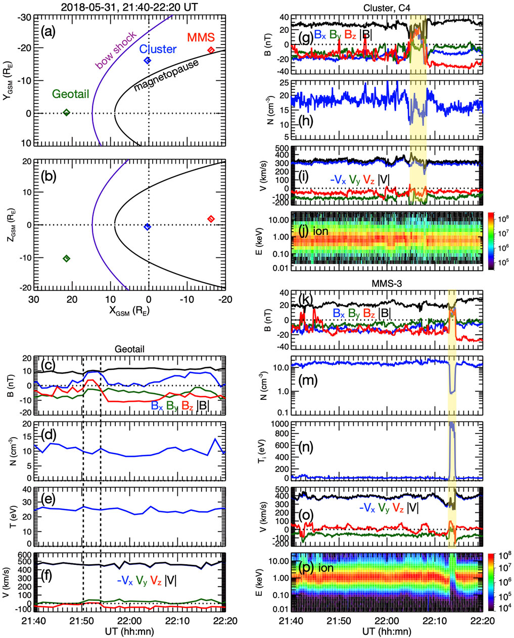
FIGURE 9. A foreshock transient event on May 31, 2018. The projections of the locations of Geotail, Cluster C4, and MMS-3 on (A) X-Y and (B) X-Z planes. Geotail observations of (C) magnetic field components, (D) number density, (E) ion temperature, and (F) ion bulk flow velocities. The two vertical dashed lines indicate the two discontinuities. Cluster observations of (G) magnetic field components, (H) number density, (I) ion bulk flow velocities, and (J) ion energy flux (eV/(s-sr-cm²-eV)). The shaded yellow and red region indicate the core and edge of the magnetosheath perturbations, respectively. MMS observations of (K) magnetic field components, (M) number density, (N) ion temperature, (O) ion bulk flow velocities, and (P) ion energy fluxes (eV/(s-sr-cm²-eV)). The shaded yellow region indicates the magnetosphere.

As the discontinuities and the magnetosheath perturbations observed at the Cluster location moved to the MMS location at ∼22:13 UT (Figure 9K), MMS observed transient appearance of the magnetosphere (yellow shaded region). The magnetosphere is indicated by that the values for the low density (Figure 9M) and high temperature (Figure 9N) within the yellow shaded region are typical for magnetospheric plasma. This change from the magnetosheath to the magnetosphere can also be seen in the sharp increases of ion fluxes at >10 keV and decreases at <2 keV shown in Figure 9P. This magnetospheric plasma seen intruding outward into the magnetosheath has substantial tailward flow speed, which is qualitatively consistent with the simulations shown in Figure 6B.

An Event for the Ionospheric Disturbances

We present in Figure 10 an observation event for ground magnetic field perturbations associated with a foreshock transient on January 20, 2010. This event has been reported by Wang et al. (2018) and they have shown simultaneous satellite observations of the event in the solar wind, foreshock, and flank magnetosheath. For this event, the driver discontinuity was observed by WIND in the solar wind. Geotail was on the dayside in the foreshock (the location is indicated in Figure 10A) and observed a transient low-density core with higher temperature and deflected flows (see Figure 4 of Wang et al. (2018) for the WIND and Geotail observations). The density perturbations observed by Geotail are shown in Figure 10A with the time of the discontinuity observed at the Geotail location indicated by the vertical magenta line. As shown in Figures 10B,C for P2 and P1, respectively, artemis P1 and P2 were both in the dawnside magnetosheath (their locations are indicated in the plots) with P2 closer to the Earth at X ∼ −27 R_E and P1 further down the tail at X ∼ −50 R_E. Figures 10A–C show that the discontinuity and the associated low-density core observed at the Geotail location at 09:04 UT propagated to P2 at ∼09:34 UT then to P1 at ∼09:39 UT.

FIGURE 10

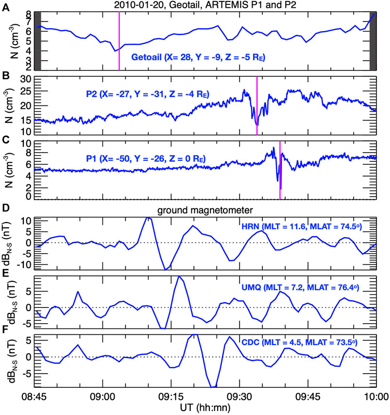
FIGURE 10. A foreshock transient event on January 20, 2010. The number density observed by (A) Geotail, (B) artemis P2, and (C) AREMIS P1. The vertical magenta line indicates the time when the IMF discontinuity was observed. The ground magnetic field perturbations (perturbations from 10-min running averages) in the north-south direction observed at (D) HRN, (E) UMQ, and (F) CDC stations.

Figures 10D–F show the ground magnetic field perturbations (obtained by subtracting the 10 min running averages) in the north-south direction observed by three magnetometer stations. The three stations were on the dawnside at similar magnetic latitudes (∼73^°–76^°) but at different MLTs from the dayside to the nightside (their MLTs and MLATs at 09:10 UT are indicated in the plots). The aurora image in N.H. from DMSP F17 satellite around 09:11 UT (not shown) indicates that the three stations were within diffuse aurora so that they were mapped to the closed field-line region of the magnetosphere. The ground magnetic field perturbations were enhanced at the three stations within the interval when the foreshock transient perturbations propagated from Geotail on the dayside to P2 and P1 on the nightside. The enhanced perturbations were first observed at ∼11 MLT, then at 07 MLT, and then 04 MLT. These simultaneous observations of the tailward propagating magnetosheath perturbations and the anti-sunward propagating ground perturbations are qualitatively consistent with the simulated anti-sunward propagating FAC perturbations in the ionosphere shown in Figure 8 generated by the simulated tailward propagating magnetopause distortion shown in Figures 1–5.

Summary and Discussion

We use the 3D global hybrid simulation results of foreshock transient perturbations driven by a TD as an example to qualitatively describe the mesoscale (in a time scale of a few minutes and a spatial scale of a few R_E) distortion of the flank magnetopause resulting from the density/pressure perturbations of the foreshock transients. After the foreshock transient perturbations propagate into the magnetosheath, the low-density core contributes to a decrease of the magnetosheath pressure (thermal pressure and dynamic pressure), which causes the magnetopause to distort locally outward. On the other hand, the high-density edge results in an increase in the magnetosheath pressure and localized inward distortion of the magnetopause. The magnetosheath perturbations propagate tailward and continue to distort the flank magnetopause. This tailward-propagating localized outward distortion qualitatively explains the transient appearance of the magnetosphere observed by satellites sitting in the flank magnetosheath. We show that the simulated flank magnetopause distortion can generate compressional magnetic field perturbations within the tail magnetosphere, which can explain the enhancements of magnetospheric ULF waves associated with foreshock transients reported in previous observation studies. As the magnetopause distortion propagates tailward, it generates FAC perturbations in the ionosphere propagating anti-sunward, which can qualitatively account for observed anti-sunward propagation of the ground magnetic field perturbations associated with the tailward propagating magnetosheath perturbations driven by foreshock transients.

The simulated magnetosheath perturbations and magnetopause distortion presented here are associated with foreshock transients generated by specific IMF and discontinuity conditions, nevertheless, we expect that they can provide a generalized and qualitative understanding of the transient and mesoscale nature of the impact on the nightside magnetopause/magnetosphere and the ionosphere since the density core and edge is the common feature to the majority of foreshock transients. In this simulation, |IMF B_y| is comparable to |IMF B_x| so that the foreshock region extends from the dayside to the nightside. Thus, as the TD propagates tailward to the nightside, it can still encounter foreshock ions so that new perturbations can be continuously generated and added into the magnetosheath. This process can be important to maintaining the significance of the magnetosheath perturbations and the corresponding flank magnetopause distortion as they propagate to the midtail. We expect that the nightside magnetosheath perturbations might become weaker in different scenarios when the IMF becomes more radial and the foreshock region is limited to the dayside. In that case, the foreshock transients entering the dayside magnetosheath would be the sole perturbations affecting the nightside magnetopause, and decay or diffuse of the perturbations during their tailward propagation would weaken their impact on the nightside. This thought experiment will be further investigated in feature simulations.

Data Availability Statement

The datasets presented in this study can be found in online repositories. The names of the repository/repositories and accession number(s) can be found below:https://doi.org/10.6084/m9.figshare.14058359.v1.

Author Contributions

C-PW is responsible for analyzing the simulation results and the two observational events. XW and YL are responsible for conducting the simulations and analysis of the simulation results. TL is responsible for analyzing the two observational events.

Funding

C.-P. Wang is supported by NASA 80NSSC19K0840. Xueyi Wang and Yu Lin are supported by NASA 80NSSC19K0840, 80NSSC17K0012, NNX17AI47G, and 80NSSC20K0604.T. Z. L. is supported by the NASA Living With a Star Jack Eddy Postdoctoral Fellowship Program, administered by the Cooperative Programs for the Advancement of Earth System Science (CPAESS). T. Z. L. is partially supported by NSF award AGS-1941012.T. Z. L. is partially supported by NSF award AGS-1941012. Computer resources for the simulations were provided by NASA Advanced Supercomputing (NAS) Division. The simulation data can be found at https://doi.org/10.6084/m9.figshare.14058359.v1.

Conflict of Interest

The authors declare that the research was conducted in the absence of any commercial or financial relationships that could be construed as a potential conflict of interest.

Publisher’s Note

All claims expressed in this article are solely those of the authors and do not necessarily represent those of their affiliated organizations, or those of the publisher, the editors and the reviewers. Any product that may be evaluated in this article, or claim that may be made by its manufacturer, is not guaranteed or endorsed by the publisher.

Supplementary Material

The Supplementary Material for this article can be found online at: https://www.frontiersin.org/articles/10.3389/fspas.2021.751244/full#supplementary-material

References

Archer, M. O., Turner, D. L., Eastwood, J. P., Horbury, T. S., and Schwartz, S. J. (2014). The Role of Pressure Gradients in Driving Sunward Magnetosheath Flows and Magnetopause Motion. J. Geophys. Res. Space Phys. 119, 8117–8125. doi:10.1002/2014JA020342

CrossRef Full Text | Google Scholar

Archer, M. O., Turner, D. L., Eastwood, J. P., Schwartz, S. J., and Horbury, T. S. (2015). Global Impacts of a Foreshock Bubble: Magnetosheath, Magnetopause and Ground-Based Observations. Planet. Space Sci. 106, 56–66. doi:10.1016/j.pss.2014.11.026

CrossRef Full Text | Google Scholar

Billingham, L., Schwartz, S. J., and Sibeck, D. G. (2008). The Statistics of Foreshock Cavities: Results of a Cluster Survey. Ann. Geophys. 26, 3653–3667. doi:10.5194/angeo-26-3653-2008

CrossRef Full Text | Google Scholar

Blanco-Cano, X., Kajdič, P., Omidi, N., and Russell, C. T. (2011). Foreshock Cavitons for Different Interplanetary Magnetic Field Geometries: Simulations and Observations. J. Geophys. Res. 116, a–n. doi:10.1029/2010JA016413

CrossRef Full Text | Google Scholar

Chu, C., Zhang, H., Sibeck, D., Otto, A., Zong, Q., Omidi, N., et al. (2017). THEMIS Satellite Observations of Hot Flow Anomalies at Earth's bow Shock. Ann. Geophys. 35 (3), 443–451. doi:10.5194/angeo‐35‐443‐2017

CrossRef Full Text | Google Scholar

Fillingim, M. O., Eastwood, J. P., Parks, G. K., Angelopoulos, V., Mann, I. R., Mende, S. B., et al. (2011). Polar UVI and THEMIS GMAG Observations of the Ionospheric Response to a Hot Flow Anomaly. J. Atmos. Solar-Terrestrial Phys. 73, 137–145. doi:10.1016/j.jastp.2010.03.001

CrossRef Full Text | Google Scholar

Hartinger, M. D., Turner, D. L., Plaschke, F., Angelopoulos, V., and Singer, H. (2013). The Role of Transient Ion Foreshock Phenomena in Driving Pc5 ULF Wave Activity. J. Geophys. Res. Space Phys. 118, 299–312. doi:10.1029/2012JA018349

CrossRef Full Text | Google Scholar

Jacobsen, K. S., Phan, T. D., Eastwood, J. P., Sibeck, D. G., Moen, J. I., Angelopoulos, V., et al. (2009). THEMIS Observations of Extreme Magnetopause Motion Caused by a Hot Flow Anomaly. J. Geophys. Res. 114, a–n. doi:10.1029/2008JA013873

CrossRef Full Text | Google Scholar

Kajdič, P., Blanco-Cano, X., Omidi, N., Meziane, K., Russell, C. T., Sauvaud, J.-A., et al. (2013). Statistical Study of Foreshock Cavitons. Ann. Geophys. 31 (12), 2163–2178. doi:10.5194/angeo-31-2163-2013

CrossRef Full Text | Google Scholar

Kajdič, P., Blanco-Cano, X., Omidi, N., Rojas-Castillo, D., Sibeck, D. G., and Billingham, L. (2017). Traveling Foreshocks and Transient Foreshock Phenomena. J. Geophys. Res. Space Phys. 122, 9148–9168. doi:10.1002/2017JA023901

CrossRef Full Text | Google Scholar

Kajdič, P., Raptis, S., Blanco‐Cano, X., and Karlsson, T. (2021). Causes of Jets in the Quasi‐Perpendicular Magnetosheath. Geophys. Res. Lett. 48, e2021GL093173. doi:10.1029/2021GL093173

CrossRef Full Text | Google Scholar

Kataoka, R., Fukunishi, H., Lanzerotti, L. J., Rosenberg, T. J., Weatherwax, A. T., Engebretson, M. J., et al. (2002). Traveling Convection Vortices Induced by Solar Wind Tangential Discontinuities. J. Geophys. Res. 107 (A12), 22-1–22-12. doi:10.1029/2002JA009459

CrossRef Full Text | Google Scholar

Lin, Y. (1997). Generation of Anomalous Flows Near the bow Shock by its Interaction with Interplanetary Discontinuities. J. Geophys. Res. 102, 24,265–24, 281. doi:10.21236/ada635320

CrossRef Full Text | Google Scholar

Lin, Y. (2002). Global Hybrid Simulation of Hot Flow Anomalies Near the bow Shock and in the Magnetosheath. Planet. Space Sci. 50, 577–591. doi:10.1016/s0032-0633(02)00037-5

CrossRef Full Text | Google Scholar

Lin, Y. (2003). Global-scale Simulation of Foreshock Structures at the Quasi-Parallel bow Shock. J. Geophys. Res. 108, 1390. doi:10.1029/2003JA009991A11

CrossRef Full Text | Google Scholar

Lin, Y., Wang, X. Y., Lu, S., Perez, J. D., and Lu, Q. (2014). Investigation of Storm Time Magnetotail and Ion Injection Using Three-Dimensional Global Hybrid Simulation. J. Geophys. Res. Space Phys. 119, 7413–7432. doi:10.1002/2014JA020005

CrossRef Full Text | Google Scholar

Lin, Y., and Wang, X. Y. (2005). Three-dimensional Global Hybrid Simulation of Dayside Dynamics Associated with the Quasi-Parallel bow Shock. J. Geophys. Res. 110, A12216. doi:10.1029/2005JA011243

CrossRef Full Text | Google Scholar

Liu, J., Lyons, L. R., Wang, C. P., Ma, Y., Strangeway, R. J., Zhang, Y., et al. (2021). Embedded Regions 1 and 2 Field‐Aligned Currents: Newly Recognized from Low‐Altitude Spacecraft Observations. J. Geophys. Res. Space Phys. 126, e2021JA029207. doi:10.1029/2021JA029207

CrossRef Full Text | Google Scholar

Liu, T. Z., Angelopoulos, V., Hietala, H., and Wilson III, L. B. (2017). Statistical Study of Particle Acceleration in the Core of Foreshock Transients. J. Geophys. Res. Space Phys. 122, 7197–7208. doi:10.1002/2017JA024043

CrossRef Full Text | Google Scholar

Liu, T. Z., Turner, D. L., Angelopoulos, V., and Omidi, N. (2016). Multipoint Observations of the Structure and Evolution of Foreshock Bubbles and Their Relation to Hot Flow Anomalies. J. Geophys. Res. Space Phys. 121, 5489–5509. doi:10.1002/2016JA022461

CrossRef Full Text | Google Scholar

Liu, T. Z., Wang, C. P., Wang, B., Wang, X., Zhang, H., and Angelopoulos, Y. V. (2020). ARTEMIS Observations of Foreshock Transients in the Midtail Foreshock. Geophys. Res. Lett. 47, e2020GL090393. doi:10.1029/2020GL090393

CrossRef Full Text | Google Scholar

Liu, Z., Turner, D. L., Angelopoulos, V., and Omidi, N. (2015). THEMIS Observations of Tangential Discontinuity‐driven Foreshock Bubbles. Geophys. Res. Lett. 42, 7860–7866. doi:10.1002/2015GL065842

CrossRef Full Text | Google Scholar

Lucek, E. A., Horbury, T. S., Balogh, A., Dandouras, I., and Rème, H. (2004). Cluster Observations of Hot Flow Anomalies. J. Geophys. Res. 109, A06207. doi:10.1029/2003JA010016

CrossRef Full Text | Google Scholar

Murr, D. L., and Hughes, W. J. (2003). Solar Wind Drivers of Traveling Convection Vortices. Geophys. Res. Lett. 30, 1354. doi:10.1029/2002GL0154987

CrossRef Full Text | Google Scholar

Omidi, N., Berchem, J., Sibeck, D., and Zhang, H. (2016). Impacts of Spontaneous Hot Flow Anomalies on the Magne- Tosheath and Magnetopause. J. Geophys. Res. Space Phys. 121, 3155–3169. doi:10.1002/2015JA022170

CrossRef Full Text | Google Scholar

Omidi, N., Eastwood, J. P., and Sibeck, D. G. (2010). Foreshock Bubbles and Their Global Magnetospheric Impacts. J. Geophys. Res. 115, A06204. doi:10.1029/2009JA014828

CrossRef Full Text | Google Scholar

Omidi, N. (2007). Formation of Cavities in the Foreshock. AIP Conf. Proc. 932, 181. doi:10.1063/1.2778962

CrossRef Full Text | Google Scholar

Omidi, N., Lee, S. H., Sibeck, D. G., Turner, D. L., Liu, T. Z., and Angelopoulos, V. (2020). Formation and Topology of Foreshock Bubbles. J. Geophys. Res. Space Phys. 125, e2020JA028058. doi:10.1029/2020JA028058

CrossRef Full Text | Google Scholar

Omidi, N., and Sibeck, D. (2007). Formation of Hot Flow Anomalies and Solitary Shocks. J. Geophys. Res. 112, A01203. doi:10.1029/2006JA011663

CrossRef Full Text | Google Scholar

Omidi, N., Zhang, H., Sibeck, D., and Turner, D. (2013). Spontaneous Hot Flow Anomalies at Quasi-Parallel Shocks: 2. Hybrid Simulations. J. Geophys. Res. Space Phys. 118, 173–180. doi:10.1029/2012JA018099

CrossRef Full Text | Google Scholar

Otto, A., and Zhang, H. (2021). Bow Shock Transients Caused by Solar Wind Dynamic Pressure Depletions. J. Atmos. Solar-Terrestrial Phys. 218, 105615. doi:10.1016/j.jastp.2021.105615

CrossRef Full Text | Google Scholar

Peredo, M., Slavin, J. A., Mazur, E., and Curtis, S. A. (1995). Three-dimensional Position and Shape of the bow Shock and Their Variation with Alfvénic, Sonic and Magnetosonic Mach Numbers and Interplanetary Magnetic Field Orientation. J. Geophys. Res. 100 (A5), 7907–7916. doi:10.1029/94JA02545

CrossRef Full Text | Google Scholar

Ridley, A. J., Gombosi, T. I., and Dezeeuw, D. L. (2004). Ionospheric Control of the Magnetosphere: Conductance. Ann. Geophys. 22 (2), 567–584. doi:10.5194/angeo-22-567-2004

CrossRef Full Text | Google Scholar

Roelof, E. C., and Sibeck, D. G. (1993). Magnetopause Shape as a Bivariate Function of Interplanetary Magnetic Field B_z and Solar Wind Dynamic Pressure. J. Geophys. Res. 98 (A12), 21,421–21,450. doi:10.1029/93JA02362

CrossRef Full Text | Google Scholar

Schwartz, S. J., Avanov, L., Turner, D., Zhang, H., Gingell, I., Eastwood, J. P., et al. (2018). Ion Kinetics in a Hot Flow Anomaly: MMS Observations. Geophys. Res. Lett. 45, 11,520–11,529. doi:10.1029/2018GL080189

CrossRef Full Text | Google Scholar

Schwartz, S. J., Chaloner, C. P., Christiansen, P. J., Coates, A. J., Hall, D. S., Johnstone, A. D., et al. (1985). An Active Current Sheet in the Solar Wind. Nature 318, 269–271. doi:10.1038/318269a0

CrossRef Full Text | Google Scholar

Schwartz, S. J. (1991). Magnetic Field Structures and Related Phenomena at Quasi-Parallel Shocks. Adv. Space Res. 11 (9), 231–240. doi:10.1016/0273-1177(91)90039-m

CrossRef Full Text | Google Scholar

Schwartz, S. J., Sibeck, D., Wilber, M., Meziane, K., and Horbury, T. S. (2006). Kinetic Aspects of Foreshock Cavities. Geophys. Res. Lett. 33 (12), 103. doi:10.1029/2005gl025612

CrossRef Full Text | Google Scholar

Shen, X.-C., Shi, Q., Wang, B., Zhang, H., Hudson, M. K., Nishimura, Y., et al. (2018). Dayside magnetospheric and ionospheric responses to a foreshock transient on 25 June 2008: 1. FLR observed by satellite and ground-based magnetometers. J. Geophys. Research: Space Phys. 123, 6335–6346. doi:10.1029/2018JA025349

CrossRef Full Text | Google Scholar

Shi, F., Lin, Y., Wang, X., Wang, B., and Nishimura, Y. (2021). 3-D Global Hybrid Simulations of Magnetospheric Response to Foreshock Processes. Earth Planets Space 73, 138. doi:10.1186/s40623-021-01469-2

CrossRef Full Text | Google Scholar

Sibeck, D. G., Borodkova, N. L., Schwartz, S. J., Owen, C. J., Kessel, R., and Kokubun, S. (1999). Comprehensive Study of the Magnetospheric Response to a Hot Flow Anomaly. J. Geophys. Res. 104, 4577–4593. doi:10.1029/1998JA900021

CrossRef Full Text | Google Scholar

Sibeck, D. G., Kudela, K., Lepping, R. P., Lin, R., Nemecek, Z., Nozdrachev, M. N., et al. (2000). Magnetopause Motion Driven by Interplanetary Magnetic Field Variations. J. Geophys. Res. 105 (A11), 25155–25169. doi:10.1029/2000JA900109

CrossRef Full Text | Google Scholar

Sibeck, D. G., Kudela, K., Mukai, T., Nemecek, Z., and Safrankova, J. (2004). Radial Dependence of Foreshock Cavities: a Case Study. Ann. Geophys. 22, 4143–4151. doi:10.5194/angeo-22-4143-2004

CrossRef Full Text | Google Scholar

Sibeck, D. G., Lee, S. H., Omidi, N., and Angelopoulos, V. (2021). Foreshock Cavities: Direct Transmission through the bow Shock. J. Geophys. Res. Space Phys. 126, e2021JA029201. doi:10.1029/2021JA029201

CrossRef Full Text | Google Scholar

Sibeck, D. G., Omidi, N., Dandouras, I., and Lucek, E. (2008). On the Edge of the Foreshock: Model-Data Comparisons. Ann. Geophys. 26, 1539–1544. doi:10.5194/angeo-26-1539-2008

CrossRef Full Text | Google Scholar

Sibeck, D. G., Phan, T.‐D., Lin, R., Lepping, R. P., and Szabo, A. (2002). Wind Observations of Foreshock Cavities: A Case Study. J. Geophys. Res. 107, 4–1. doi:10.1029/2001ja007539

CrossRef Full Text | Google Scholar

Thomsen, M. F., Gosling, J. T., Fuselier, S. A., Bame, S. J., and Russell, C. T. (1986). Hot, Diamagnetic Cavities Upstream from the Earth’s bow Shock. J. Geophys. Res. 91, 2961–2973. doi:10.1029/JA091iA03p02961

CrossRef Full Text | Google Scholar

Turner, D. L., Liu, T. Z., Wilson, L. B., Cohen, I. J., Gershman, D. G., Fennell, J. F., et al. (2020). Microscopic, Multipoint Characterization of Foreshock Bubbles with Magnetospheric Multiscale (MMS). J. Geophys. Res. Space Phys. 125, e2019JA027707. doi:10.1029/2019JA027707

CrossRef Full Text | Google Scholar

Turner, D. L., Omidi, N., Sibeck, D. G., and Angelopoulos, V. (2013). First Observations of Foreshock Bubbles Upstream of Earth's bow Shock: Characteristics and Comparisons to HFAs. J. Geophys. Res. Space Phys. 118, 1552–1570. doi:10.1002/jgra.50198

CrossRef Full Text | Google Scholar

Wang, B., Liu, T., Nishimura, Y., Zhang, H., Hartinger, M., Shi, X., et al. (2020). Global Propagation of Magnetospheric Pc5 ULF Waves Driven by Foreshock Transients. J. Geophys. Res. Space Phys. 125, e2020JA028411. doi:10.1029/2020JA028411

CrossRef Full Text | Google Scholar

Wang, B., Nishimura, Y., Hietala, H., Lyons, L., Angelopoulos, V., Plaschke, F., et al. (2018a). Impacts of Magnetosheath High-Speed Jets on the Magnetosphere and Ionosphere Measured by Optical Imaging and Satellite Observations. J. Geophys. Res. Space Phys. 123, 4879–4894. doi:10.1029/2017JA024954

CrossRef Full Text | Google Scholar

Wang, B., Nishimura, Y., Hietala, H., Shen, X.‐C., Lyons, L., Angelopoulos, V., et al. (2019). The 2‐D Structure of Foreshock‐driven Field Line Resonances Observed by THEMIS Satellite and Ground‐based Imager Conjunctions. J. Geophys. Res. Space Phys. 124, 6792–6811. doi:10.1029/2019JA026668

CrossRef Full Text | Google Scholar

Wang, B., Nishimura, Y., Hietala, H., Shen, X.‐C., Shi, Q., Zhang, H., et al. (2018b). Dayside Magnetospheric and Ionospheric Responses to a Foreshock Transient on 25 June 2008: 2. 2-D Evolution Based on Dayside Auroral Imaging. J. Geophys. Res. Space Phys. 123, 6347–6359. doi:10.1029/2017JA024846

CrossRef Full Text | Google Scholar

Wang, B., Zhang, H., Liu, Z., Liu, T., Li, X., and Angelopoulos, V. (2021). Energy Modulations of Magnetospheric Ions Induced by Foreshock Transient‐Driven Ultralow‐Frequency Waves. Geophys. Res. Lett. 48, e2021GL093913. doi:10.1029/2021GL093913

CrossRef Full Text | Google Scholar

Wang, C. P., Liu, T. Z., Xing, X., and Masson, A. (2018). Multispacecraft Observations of Tailward Propagation of Transient Foreshock Perturbations to Midtail Magnetosheath. J. Geophys. Res. Space Phys. 123, 9381. doi:10.1029/2018JA025921

CrossRef Full Text | Google Scholar

Wang, C. P., Thorne, R., Liu, T. Z., Hartinger, M. D., Nagai, T., Angelopoulos, V., et al. (2017). A Multispacecraft Event Study of Pc5 Ultralow‐frequency Waves in the Magnetosphere and Their External Drivers. J. Geophys. Res. Space Phys. 122, 5132–5147. doi:10.1002/2016JA023610

CrossRef Full Text | Google Scholar

Wang, C. P., Wang, X., Liu, T. Z., and Lin, Y. (2021). A Foreshock Bubble Driven by an IMF Tangential Discontinuity: 3D Global Hybrid Simulation. Geophys. Res. Lett. 48, e2021GL093068. doi:10.1029/2021GL093068

CrossRef Full Text | Google Scholar

Wang, C. P., Wang, X., Liu, T. Z., and Lin, Y. (2020). Evolution of a Foreshock Bubble in the Midtail Foreshock and Impact on the Magnetopause: 3‐D Global Hybrid Simulation. Geophys. Res. Lett. 47, e2020GL089844. doi:10.1029/2020GL089844

CrossRef Full Text | Google Scholar

Zhang, H., Le, G., and Sibeck, D. G. (2017). MMS Observations of a Hot Flow Anomaly in the Magnetosheath. American Geophysical Union, Fall Meeting 2017, abstract #SM11B-230.

Zhang, H., Sibeck, D. G., Zong, Q.-G., Gary, S. P., McFadden, J. P., Larson, D., et al. (2010). Time History of Events and Macroscale Interactions during Substorms Observations of a Series of Hot Flow Anomaly Events. J. Geophys. Res. 115, A12235. doi:10.1029/2009JA015180

CrossRef Full Text | Google Scholar

Zhang, H., Sibeck, D. G., Zong, Q.-G., Omidi, N., Turner, D., and Clausen, L. B. N. (2013). Spontaneous Hot Flow Anomalies at Quasi-Parallel Shocks: 1. Observations. J. Geophys. Res. Space Phys. 118, 3357–3363. doi:10.1002/jgra.50376

CrossRef Full Text | Google Scholar

Zhang, H., and Zong, Q. (2020). “Transient Phenomena at the Magnetopause and Bow Shock and Their Ground Signatures,” in Dayside Magnetosphere Interactions. Editors Q. Zong, P. Escoubet, D. Sibeck, G. Le, and H. Zhang, 11–37. doi:10.1002/9781119509592.ch2

CrossRef Full Text | Google Scholar