Ion Dynamics in the Meso-scale 3-D Kelvin–Helmholtz Instability: Perspectives From Test Particle Simulations

1 Introduction

The Kelvin–Helmholtz (KH) instability is one of the most common physical processes at the magnetopause boundary of the Earth (Fairfield et al., 2000; Hasegawa et al., 2004; Nykyri et al., 2006; Eriksson et al., 2016; Li et al., 2016) as well as other planets (e.g., Jupiter and Saturn) (Johnson et al., 2014; Ma et al., 2015; Burkholder et al., 2017). It is driven by a large sheared flow, and it can be stabilized by the magnetic field along the sheared flow direction (Chandrasekhar, 1961), compressibility, and a broad initial shear flow width (Miura and Pritchett, 1982). Therefore, KH instability can occur under north, south, and Parker-spiral interplanetary magnetic field (IMF) conditions in the vicinity of the equatorial plane (Hwang et al., 2011; Kavosi and Raeder, 2015; Henry et al., 2017), as well as at high latitudes during the dawn or dusk-ward IMF condition (Hwang et al., 2012; Ma et al., 2016; Nykyri et al., 2021a).

As a macro-scale dissipation process, the KH instability alone can transport momentum and energy from solar wind into the magnetosphere (Pu and Kivelson, 1983a; Pu and Kivelson, 1983b). It has been shown that the anomalous (eddy) viscosity is about 0.02V₀a in the nonlinear stage of the KH instability, where a is the half width of the initial velocity shear layer, and V₀ is total velocity jump (Miura, 1984), which is about 10⁹ m² s⁻¹ for a typical Earth’s magnetopause condition. This value is consistent with the requirement by the “viscous-like” interaction (Axford and Hines, 1961; Sonnerup, 1980). Furthermore, during the nonlinear stage, the KH instability can strongly modify the boundary, generating a thin current sheet, which triggers magnetic reconnection (Otto and Fairfield, 2000; Nakamura et al., 2008; Nakamura and Fujimoto, 2008) and other kinetic physics [e.g., kinetic Alfvén wave, magnetosonic wave, see detailed discussion in (Masson and Nykyri, 2018)]. These secondary processes will break the frozen-in condition which allows the plasma transport between the magnetosheath and the magnetosphere (Otto and Fairfield, 2000; Nakamura et al., 2008; Ma et al., 2017). In two-dimensional (2-D) geometry, there are two types of KH driven reconnection (Nakamura et al., 2008; Nakamura and Fujimoto, 2008). “Type I” operates if the initial magnetic field component along the sheared flow direction is anti-parallel across the sheared flow layer (i.e., a pre-existing large current layer case). In this condition, the pre-existing current layer will be further compressed in the spine region (i.e., the region connecting two neighboring vortices) during the growth of the KH instability, and this process will eventually trigger magnetic reconnection. This reconnection process allows the magnetosheath magnetic field to connect to magnetospheric magnetic field. The “type II” operates without a pre-existing current layer, meaning the magnetic field components across the sheared flow layer are mostly along the same direction. In such a condition, the well developed KH vortices can fold the magnetic field line in the KH plane (Otto and Fairfield, 2000). This process can change the magnetic field directions and form thin current layers in the vortices. If the width of the current layer is comparable to the ion inertial length, then magnetic reconnection occurs between the magnetosheath field lines or the magnetospheric field lines, which generates a large magnetic island detached from the original field line which moves to the other side of the original boundary layer. Two-dimensional MHD and Hall MHD estimated that this type of plasma transport process can transport plasma at a speed of several km s⁻¹, equivalent to a diffusion coefficient of about 10⁹ m² s⁻¹ for Earth’s typical magnetopause conditions (Nykyri and Otto, 2001; Nykyri and Otto, 2004). Although hybrid simulations show similar overall dynamical properties (e.g., growth rate, anomalous (eddy) viscosity, and the size of mixed region), magnetic reconnection occurs in a more patchy manner, which forms a series of smaller magnetic islands (Ma et al., 2019). In order to quantify the diffusion caused by the nonlinear KH instability, hybrid simulations define mixing region based on the percentage of the particles from both side of the boundary in a given cell (Terasawa et al., 1992), or calculate the standard deviation of the normal direction displacement of the particles in the activity region (Cowee et al., 2009; Cowee et al., 2010). For hybrid simulation, the mixing diffusion coefficient is about 10⁸—10⁹ m² s⁻¹ for typical Earth’s environment (Cowee et al., 2009; Cowee et al., 2010) and 10¹⁰ m² s⁻¹ for Saturn (Delamere et al., 2011).

The observed KH instability at the 3-D magnetopause boundary is often localized in the vicinity of the equatorial plane due to the magnetic field curvature. For northward IMF condition, the well developed KH vortex will drag low-latitude magnetosheath magnetic field lines in the sun-ward direction and low-latitude magnetospheric magnetic field lines in the tail-ward direction, reminiscent of a “candy wrapper.” This process will generate anti-parallel magnetic field components at mid-latitude, and eventually will trigger a pair of mid-latitude reconnection sites, which is often referred as double-mid-latitude-reconnection (DMLR) (Otto, 2006; Faganello et al., 2012). Detailed discussions of type-I, type-II, and DMLR can be found in recent papers by Faganello and Califano (Faganello and Califano, 2017) and Ma et al. (Ma et al., 2017). The net effect of this process exchanges the low-latitude magnetosheath and magnetospheric flux tubes, and therefore transports the mass and flux tube entropy between the magnetosheath and the magnetosphere. It has been estimated that the mass transport rate is about 10¹⁰ m² s⁻¹ (Ma et al., 2017) for Earth’s typical magnetopause condition. For southward IMF condition, the KH instability can occur on the equatorial plane, while the meridian is tearing mode unstable. Thus, both KH instability and magnetic reconnection can operate simultaneously. The nonlinear interaction between these two processes leads to a fast reconnection growth rate which is close to the Petschek reconnection rate without including kinetic physics. However, the total reconnected flux is limited by the KH instability, since the KH instability diffuses the boundary current layer (Ma et al., 2014a; Ma et al., 2014b).

It is also useful to consider the KH instability as a cross-scale process. The typical KH wavelength at the Earth’s magnetopause is about 2–6 Earth’s radii (R_E), (i.e., about 50–500 ion inertial lengths for the magnetopause density around 1–10 cm⁻³), and the localization along the z direction is comparable to the KH wavelength (Ma et al., 2014a). However, the different types of secondary instabilities triggered by the nonlinear KH instability often occur at sizes comparable to ion inertial scales (Nykyri et al., 2021b). Thus, it would be ideal to use hybrid or even fully kinetic simulation to systematically investigate the KH instability and its secondary instability. For instance, Karimabadi et al. (Karimabadi et al., 2013) used kinetic PIC code VPIC to demonstrate the formation of coherent structures in the form of current sheets that steepen to electron scales through turbulent cascade during the KH instability, which triggers strong localized heating of the plasma. However, it is often computationally expensive and the non-periodic boundary conditions along the non-wave-direction are not trivial to incorporate in particle simulations.

One compromise is the test particle simulation approach based on the electromagnetic field provided by fluid simulation. This approach does not provide a feedback mechanism from particles to the field, such that a significant part of the kinetic physics aspect is excluded. However, it still reproduces the anisotropic temperature and particle mixing in a two-dimensional geometry (Ma et al., 2019). Furthermore, Henri et al. (Henri et al., 2013) carefully compared simulation of 2-D KH instability by using MHD, Hall-MHD, two-fluid, hybrid kinetic, and full kinetic codes, showing that the feedback from small, kinetic scales to large, fluid scales is negligible in the nonlinear regime despite differences in the small scale processes between the different models. Thus, the motivation of this paper is to further explore the application of the test particle simulation in a 3-D KH instability.

2 Numerical Method

2.1 MHD Simulation

In this study, all physical quantities are normalized by their typical values, which are given by length scale L₀ = 640 km, density n₀ = 10 cm⁻³, magnetic field magnitude B₀ = 70 nT, and the typical value of other quantities can be derived from these three quantities. The full set of normalized resistive MHD equations are solved by the leap-frog scheme, which has a long heritage of investigating mesoscale MHD instabilities (Birn, 1976; Otto, 1990; Otto and Fairfield, 2000; Nykyri and Otto, 2001; Ma et al., 2014a; Ma et al., 2014b; Ma et al., 2017). The whole set of simulations are carried out in a rectangular cuboid domain (i.e., [−L_x, L_x] × [−L_y, L_y] × [−L_z, L_z]), in which L_x = 20, L_y = 10, and L_z = 40. Here the x direction is the normal direction of the unperturbed magnetopause boundary, pointing from the magnetosphere to the magnetosheath. The z direction points to the North, which is mostly along the magnetic field direction. The y direction is determined by the right hand rule, which is also mostly along the sheared flow direction. The y direction uses periodic boundary conditions. The x direction uses closed boundary conditions (i.e., B_x = v_x = 0 and ∂_x = 0 for other quantities), however, the dimension along the x direction is sufficiently large, that the reflection from x boundary is negligible to the end of the simulation. The z direction uses open boundary conditions (i.e., ∂_z = 0 for all quantities, except B_z is determined by the zero-divergence of the magnetic field), however quantities on these boundaries remain at their initial value due to the artificial friction term we applied to the top and bottom boundaries (see below).

The initial steady state configuration is a one-dimensional transition layer, which is given by $\mathbf{F}=\bar{\mathbf{F}}+\delta \mathbf{F}\tanh (x/D)$, where D = 1 is the width of the transition layer, F = [ρ, v_y, B_y, B_z], $\bar{\mathbf{F}}={\mathbf{F}}_1+{\mathbf{F}}_2$, and δF = F₁ − F₂. Here, the subscripts 1 and 2 represent the value on the magnetosheath side (i.e., x > 0) and the magnetospheric side (i.e., x < 0), respectively. The other components of the vector quantities are set to be zero (i.e., v_x = v_z = B_x = 0). Two different initial conditions are used in this study. The first case is given by F₁ = [1.54, 0.42, 0, 1.02] and F₂ = [0.46, 0.42, 0, 0.98], which is referred to as the symmetric case since B_y = 0. In this situation, the bulk velocity is perpendicular to the magnetic field. In a 2-D geometry, the dynamics in the xy-plane decouple from the z direction, which eliminates the onset of magnetic reconnection in the MHD and hybrid description (Otto and Fairfield, 2000; Settino et al., 2020). In the 3-D geometry, the system maintains north-south symmetry, meaning the magnetic field is always perpendicular to the bulk flow in the equatorial plane. Thus, there is no low-latitude reconnection (Ma et al., 2017). However, the localized perturbation and boundary condition (see below) break the translational symmetry along the z direction, which locally twists the magnetic field to generate DMLR (Faganello et al., 2012; Faganello and Califano, 2017; Ma et al., 2017). The second case is given by F₁ = [1.54, 0.42, −0.35, 1.02] and F₂ = [0.46, 0.42, −0.08, 0.98], which is referred to as the asymmetric case and low-latitude KH driven reconnection can occur. The initial conditions for the asymmetric case are approximately the same as those observed by the MMS satellites on 8 Sept 2015 (Eriksson et al., 2016). Notice, this event has been simulated by several numerical models, which mostly use a constant B_z [e.g., (Nakamura et al., 2017; Franci et al., 2020)]. Due to the flexility of the MHD model, we can include a tiny B_z variation in this study to make the model closer to the real event. However, such a tiny variation is not expected to bring a significant impact on the overall dynamics compared to the constant B_z.

The KH instability is triggered by a velocity perturbation, which is given by v = ∇Φ(x, y) × e_z f(z). Here, the stream function is Φ(x, y) = δv cos(x/l_x) cosh⁻¹(k_yy), l_x = 2, k_y = π/L_y and δv = v_y/20. In this study, the simulation assumes the high-latitude magnetic field lines move with the solar wind or are tied to the ionosphere. Thus, the KH perturbation is localized in the vicinity of the equatorial plane, in which the localization function f(z) is given by f(z) = 0.5{ tanh[(z + z_d)/D_z] − tanh[(z − z_d)/D_z]}, z_d = 0.5L_z, and D_z = 3. Furthermore, an artificial friction term − ν(z)(v − v₀) is applied to the right-hand side of the momentum equation. Here, v₀ is the unperturbed bulk velocity, which also represents the solar wind or ionosphere speed. The friction term tends to force the plasma to move at its initial velocity, or equivalently it absorbs perturbations, maintaining the initial boundary layer away from the equatorial plane. Therefore, the friction coefficient is given by ν(z) = 0.5{2 − tanh[(z + z_ν)/D_ν] + tanh[(z − z_ν)/D_ν]}, z_ν = 0.75L_z, and D_ν = 3, which has been switched on only near the top and bottom boundaries (Ma et al., 2017).

In the MHD simulation, for any given point at any given time, a magnetic field line can be traced from this point to the top and bottom boundaries. Notice, the top and bottom boundaries in this simulation represent the unperturbed region. Thus, if the x-component of the spatial location of the magnetic field line’s footprint on the top (X_top) or bottom boundaries (X_bot) is smaller than zero, then it means this end of the magnetic field line is connecting to the magnetospheric side at that moment. Similarly, if the X_top or X_bot is larger than zero, then it means this end of the magnetic field line is connecting to the magnetosheath side. In this study, we refer to the magnetic field line with both top and bottom footprints on the magnetosheath (magnetospheric) side as magnetosheath (magnetospheric) field lines. Magnetic field line with one end connecting to the magnetosheath side and the other end connecting to the magnetospheric side is referred to as open field line.

2.2 Test Particle Simulation

The full set of non-relativistic Lorentz equations are solved using the traditional Boris method (Boris, 1970), which has been used to investigate high-energy particles in the cusp diamagnetic cavity (Nykyri et al., 2012), and KH instability (Ma et al., 2019). The symmetric treatment of the time derivative in the Boris method maintains the temporal reversibility of the Lorentz equation. Thus, this code can reverse trace the test particles to reconstruct particle distributions based on Liouville’s theory (Birn et al., 1997; Birn et al., 1998).

For the forward tracing simulation, we launch particles with shifted Maxwellian distributions (max v < 4 in simulation unit or 2000 km s⁻¹) inside of the MHD simulation domain (i.e., [−15, 15] × [−10, 10] × [−40, 40]) with 150 × 200 × 200 cells at t = 0, which covers most of the KH active region. Notice, we did not launch the particles outside of |x| = 15 to save on computational effort, since the thermal particles there merely reach to the KH active region toward the end of the simulation. The number of particles in each cell is proportional to the plasma density in the middle of the cell (i.e, 50 particles/cell ∼ ρ = 0.46), which gives a total 6,51,320,000 particles within the MHD simulation domain. The number of particles on the magnetospheric side is about 1/3 of the particles on the magnetosheath side. Maintaining particle numbers in the simulation domain is an important aspect of particle simulations (i.e., PIC, hybrid, and test particle simulation), in which periodic boundary conditions are often used. However, the 3-D KH instability processes, which involves middle latitude reconnection or nonlinear interaction between the KH instability and reconnection processes have no periodicity along the third direction (i.e., z-direction). Therefore, the often used periodic boundary conditions may not be appropriate for these types of simulations. This study uses extended boundary conditions. This type of boundary condition adds additional domains ([−dL_z − L_z, L_z + dL_z]) along the top and bottom of the fluid simulation domains ([−L_z, L_z]), in which density, pressure, magnetic field, and bulk velocity are set to be the same as the value at the fluid simulation top and bottom boundaries. Consequently, the particle distribution is initialized in the same way as it is inside of the fluid simulation domain. For computational efficiency, we only trace the particles that can reach the simulation domain during the test particle simulation time. Those particles can be easily identified by their initial location z₀ and velocity v₀. Assuming that the total test particle simulation interval is τ and the charged particles are mostly moving along the magnetic field line (at least in the buffer region), then by the time of τ, the z component of the particle location will be within $z_e=z_0+v_{0\parallel }\tau \pm g_r=z_e^{\prime }\pm g_r$, where v_0∥ is the initial parallel velocity, and g_r is the gyro-radius, which is dependent on the initial perpendicular velocity. Notice, if B_y ≠ 0, the gyro motion has a component along the z direction, which is the reason why we have to take the gyro-radius in to account. Thus, we only need to trace particles with $|z_e^{\prime }|<L_z+\delta z$, where δz is an arbitrary value greater than max g_r. During this study, this boundary condition leads to the total number of particles inside of the simulation box [−L_z, L_z] changing less than 0.4% of the initial number.

For the backward tracing, we only focus on the KH active region in the equatorial plane (i.e., [−6, 6] × [−10, 10] resolved by 61 × 101 grid points) in the nonlinear stage for the symmetric case. For each individual grid point, we traced 51³ particles backward to t = 0, covering a range of ${[-3v_{th},3v_{th}]}^3$ in velocity space. Here, v_th is the thermal velocity at the grid point. Then, the weight of each particle, w, is estimated based on the phase space density of the shifted Maxwellian distribution at [x,v]_t=0 with the assumption that Liouville’s theory is satisfied. Thus, the number density, velocity, and pressure can be obtained through the zeroth to second order moments of w integrated over the whole ${[-3v_{th},3v_{th}]}^3$ velocity space.

3 Results

Figure 1 shows a fully developed KH vortex in the equatorial plane (z = 0) at t = 130 for the symmetric case (top) and the asymmetric case (bottom). The black arrows are the bulk velocity. The color index represents the plasma density, ρ, (left) and mixing rate, r_M, (right). Here, the high and low density regions indicate the magnetosheath plasma and the magnetospheric plasma, respectively. The mixing rate is defined as r_M = 1–2|0.5 − p|, where 1 ≥ p ≥ 0 is the probability of magnetosheath particles for a given cell (Matsumoto and Hoshino, 2006). Thus r_M = 1 means fully mixed, r_M = 0 means no mixing. The magenta line represents the magnetosheath-magnetosphere boundary based on magnetic field topology (i.e., the x-component of the magnetic field line footprints on the top or bottom boundaries are zero). Thus, for the symmetric case all the magnetic field lines on left side of the magenta line are closed magnetospheric field lines, which also includes regions with magnetosheath-like, high-density plasma. Magnetic field lines in these regions have experienced the DMLR process, changing their connection from the magnetosheath to the magnetosphere, which are referred to as “newly connected magnetospheric magnetic field lines.” Similarly, magnetospheric-like, low-density plasma also observed on the right side of the magenta line, indicating that magnetic field lines in these regions are “newly connected magnetosheath magnetic field lines.” For the asymmetric case, a single magnetic field line may not experience DMLR simultaneously, which will generate open flux regions (e.g., y ∈ [2,4] region). The right panels of mixing rate r_M show that the majority of the mixed region is along the density boundary layer. Note, some newly connected magnetospheric magnetic field lines do not involve any mixing. This means the mixing in the low latitude is mostly via the finite gyroradius effect. Although the DMLR process provides the connection between magnetosheath and magnetospheric field lines, it takes time for ion particles moving from high latitudes to lower latitudes to influence the mixing rate in the equatorial plane.

FIGURE 1

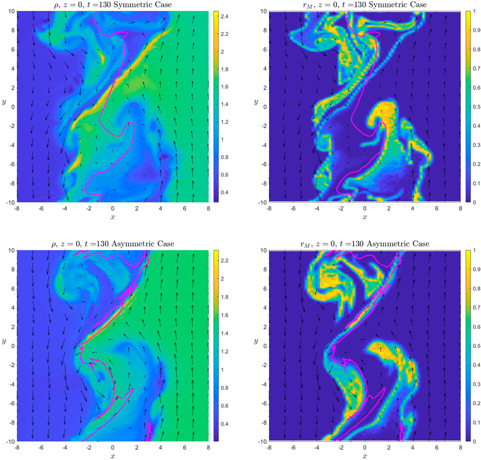
FIGURE 1. A fully developed KH vortex in the equatorial plane (z = 0) at t = 130 for the symmetric case (top) and the asymmetric case (bottom). The color index represents the plasma density (left) and mixing rate (right). The black arrows represent the x and y components of the bulk velocity. The magenta line represents the magnetosheath-magnetosphere boundary based on magnetic field topology.

Figure 2 shows the overall dynamic properties for the symmetric case (left) and the asymmetric case (right). The top to bottom panels plot the growth of the KH instability (the range of the bulk velocity v_x component), the change of mass on the magnetosheath side (blue) and magnetospheric side (red), and the total mixed volume V_m = ∫r_M(x, y, z)dxdydz, respectively. This demonstrates that the perturbation grows exponentially before t = 80 (i.e., the linear stage) and saturates after t = 80 (i.e., the nonlinear stage) for the symmetric case. Stabilized by the magnetic B_y component, the asymmetric case has a relatively lower growth rate. During the nonlinear stage, a significant amount of mass is transported from the magnetosheath into the magnetosphere via the DMLR process for the symmetric case. We estimated that the maximum transport rate (i.e., dM/dt) is about 10²⁵ particles/s, or the transport diffusion coefficient of 9 × 10⁹ m² s⁻¹, which is given by $d{L}_M^2/dt$, where L_M = M/(4L_yL_zρ_msh). For the asymmetric case, the plasma lost from the magnetosheath side moves to the magnetospheric side as well as to open flux regions. Thus, the magnetosheath mass decrease rate is comparable to the symmetric case, while the magnetosphere mass increase rate is lower than it is in the symmetric case. Actually, at the early stage, the magnetosphere loses mass into the open flux region, due to the DMLR process operating nonsimultaneously. The total mixed volume, V_m, also shows a significant increase during the nonlinear stage, which is due to the elongation of the magnetosheath-magnetosphere boundary layer via the KH vortex as well as magnetic field line topology change via the mid-latitude reconnection process. While the asymmetric case shows a much smaller total mixed volume than the symmetric case by the time t = 130, it could be simply due to the asymmetric case reaching the nonlinear stage a bit later than the symmetric case. The maximum mixing diffusion rate for the symmetric case is about 1010 m² s⁻¹, given by $d{L}_m^2/dt$, where L_m = V_m/(4L_zL_y).

FIGURE 2

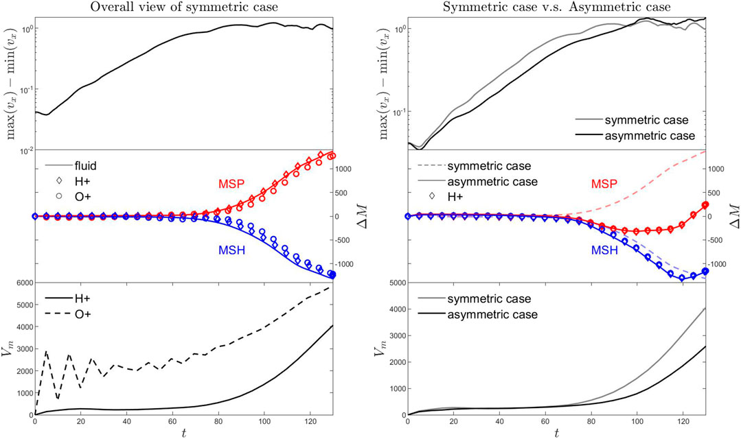
FIGURE 2. The overall dynamical properties for the symmetric case (left) and the asymmetric case (right). The top to bottom panels show the growth of the KH instability (the range of the bulk velocity v_x component), the change of mass on the magnetosheath side (blue) and magnetospheric side (red), and the total mixed volume V_m, respectively. In the left-middle panel, the fluid approach is represented by the solid lines and test particle approaches based on H+ and O+ are represented by diamonds and circles, respectively. In the left-bottom panel the total mixed volume is shown based on H+ (solid line) and O+ (dashed line). In the right panels, the results from symmetric case are in light gray lines or dashed lines for reference.

In this study, we apply both fluid and particle approaches to evaluate the total mass on the magnetosheath side and the magnetospheric side. For the fluid approach, one can trace the magnetic field lines from the top of the MHD simulation domain, and calculate the flux tube content η(x, y) = ∫ρ/Bds along the magnetic field line, then integrate the flux tube content on the top boundary on the magnetosheath (i.e., M_msh = ∫_mshη(x, y)B_zdxdy) and magnetospheric sides (M_msp = ∫_mspη(x, y)B_zdxdy). This method is computationally inexpensive, however it may incur a large error if the boundary is not perfectly unperturbed. A more accurate method is to integrate the plasma density in the magnetosphere, magnetosheath, and open flux regions (i.e., M = ∫ρdxdydz), which can be achieved via identification of the connection of each grid point (magnetosphere, magnetosheath or open flux) by tracing the field lines to the top and bottom boundaries. A dense grid is needed in the KH active region to increase the accuracy, which requires a relatively higher computational cost. For the particle approach, one can count the total number of particles with different connections. However, this is a computationally expensive. A more practical approach is to identify the x-component of footprints on the top (X_top) and bottom (X_bot) boundary for each individual grid point of a dense grid covering the KH active region, and then interpolate the X_top and X_bot to the guiding center of the particle to identify the connection of each individual particle. One can also redistribute the particles to the eight neighboring grid points to get a smoother statistical count. However, with a large number of particles, these two methods give almost identical results. As long as we know the total mass each particle represents, we can easily covert the particle approach (number of particles) into the fluid approach (mass). The middle panel of Figure 2 shows the results from the fluid approach (solid lines) and particle approach (diamond) are identical, indicating the zeroth order moment of the particle distribution is consistent with the fluid description.

In this study, we launch two different ion species (i.e., H+ and O+) with the same velocity distribution for the symmetric case. The result (left-middle panel in Figure 2) shows that although O+ (circle) has a much larger gyroradius compared to H+ (diamond), it is still much smaller than the KH wavelength. Thus, the transport rate is insensitive to the mass-to-charge ratio for Earth’s typical magnetopause conditions. The left-bottom panel of Figure 2 shows that with a much larger gyroradius, the mixed volume for O+ (dashed line) is much greater than the H+ (solid line). In the linear stage, the ratio between O+ and H+ mixed volume is close to the ratio of their gyroradii, with the oscillation in the dashed line caused by the O+ gyro-frequency. However, in the nonlinear stage the O+ and H+ mixed volumes have a similar mixing diffusion rate, and their ratio decreases to about two. This is because in the nonlinear stage the density boundary is highly twisted and folded by the KH instability, collapsing the original undulated boundary layer into a thick region, which limits the efficiency of the larger gyroradius on the increase of the mixed volume.

The large temperature and specific entropy difference between the magnetosheath and magnetospheric plasma leads to an important question of whether the plasma has been (nonadiabatically) heated when it is transported from the magnetosheath into the magnetosphere (Ma and Otto, 2014). It has been demonstrated that magnetic reconnection cannot provide sufficient adiabatic heating unless the plasma beta is much smaller than unity (Ma and Otto, 2014). However, the typical magnetosheath plasma beta is about one (Ma et al., 2020), leading to the speculation that the KH instability may be responsible for an additional nonadiabatic heating source (Moore et al., 2016; Moore et al., 2017; Nykyri et al., 2021a; Nykyri et al., 2021b). But, as an ideal instability (i.e., the onset of the instability does not break the “frozen-in” condition), the MHD description of the KH instability conserves specific entropy, meaning no nonadiabatic heating source. Nevertheless, the KH instability and the associated secondary instabilities are naturally associated with turbulence (Matsumoto and Hoshino, 2006; Stawarz et al., 2016; Nakamura et al., 2017; Nykyri et al., 2017; Dong et al., 2018; Nakamura et al., 2020), which has a long history of studies demonstrating that turbulent heating is a very effective mechanism for ion heating [e.g., Quataert (Quataert, 1998), Johnson and Cheng (Johnson and Cheng, 2001), Chandran et al. (Chandran et al., 2010), Told et al. (Told et al., 2015), Vasquez (Vasquez, 2015), Grošelj et al. (Grošelj et al., 2017), Arzamasskiy et al. (Arzamasskiy et al., 2019), Cerri et al. (Cerri et al., 2021)]. Delamere et al. (Delamere et al., 2021) estimated a turbulent ion heating rate density ≈10^–15 W m⁻³ during the nonlinear stage of 3-D hybrid KH instability simulations based on the typical Saturn’s magnetopause boundary condition, which is consistent with the Cassini data analysis (Burkholder et al., 2020). Such estimations should also apply to investigate Earth’s magnetopause boundary both from numerical simulation and observational data analysis, which, however, is out of scope of this paper. Meanwhile, from the perspective of the particle description, there are two plausible hypotheses to increase the specific entropy. The first one is the free expansion of magnetosheath plasma into the newly reconnected magnetosphere flux tube (Johnson et al., 2014). The second one is that higher energy particles are preferentially transported from magnetosheath into the magnetosphere by the KH instability, which can be easily tested by using test particle simulation. Recently, MMS encountered trapped energetic particles within KH waves at the high-latitude magnetosphere (Nykyri et al., 2021a).

The top panel of Figure 3 plots the energy distribution for the particles that moved from the magnetosheath into the magnetosphere (blue) and the particles that moved from the magnetosphere into the magnetosheath (red) at t = 130 for the symmetric case. As a reference, we also plot the energy distribution for those particles at t = 0 (dots), as well as the energy distribution for the particles remaining in the magnetosphere (black) and the magnetosheath (magenta). Here, the energy is $v_d^2$, where v_d is the particle velocity minus the MHD bulk velocity. The results show the energy distributions do not change with the time, indicating there is no heating source during the KH process, which is consistent with the MHD description. However, the mean energy (i.e., temperature) of the plasma transported from the magnetosheath into the magnetosphere is indeed higher than the plasma remaining in the magnetosheath, and particles transported from the magnetosphere to the magnetosheath are lower energy than those remaining in the magnetosphere. This appears to support that the KH instability filters higher energy particles from magnetosheath into the magnetosphere. However, the bottom panel of Figure 3 plots the initial energy distribution (i.e., t = 0) for the particles that already crossed the boundary at t = 130 as a function of their initial location along the x-direction. The black line represents 1.5 times the initial temperature, T (i.e., kinetic energy), demonstrating that the higher energy (temperature) of the magnetosheath-originating particles is simply because they are from the hotter part of the preexisting boundary layer. Thus, the second hypothesis does not hold for the thermal population. The super-thermal population requires additional testing, which is out of the scope of this study.

FIGURE 3

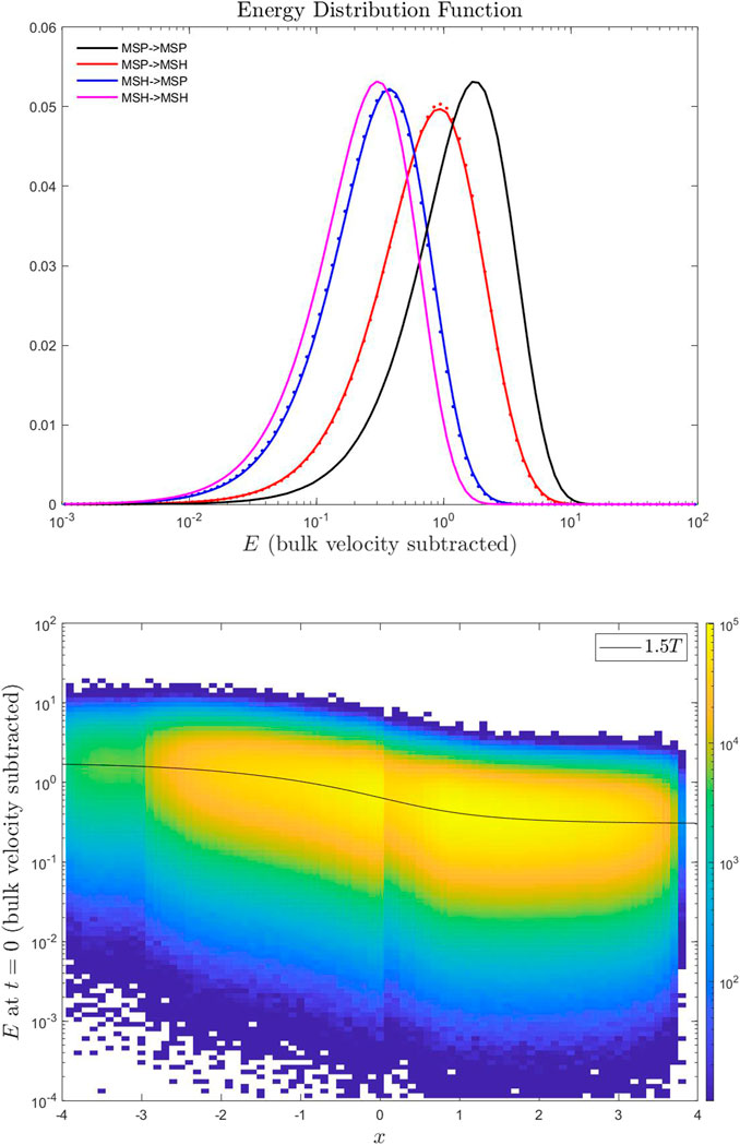
FIGURE 3. The top panel shows the energy distribution (see text) for four different types of particles (see legend) from the symmetric case. The solid lines represent those particles’ energy distribution at t = 130, while the dotted lines represent those particles’ energy distribution at t = 0. The bottom panel shows the initial energy distribution as a function of their initial location (x-component) for the particles crossing between the magnetosphere and the magnetosheath. The black line shows the energy-associated with initial temperature 1.5T.

The above results suggest that the zeroth order moment of the particle distribution in the whole simulation domain is mostly consistent with the density from the MHD simulation. It is of interest to examine the consistency of higher order moments between test particle and MHD simulation. The top panels of Figure 4 plot the deviation between MHD bulk velocity, v_M and the first order moment from forward tracing (v_F, left) and backward tracing (v_B, right) in the equatorial plane z = 0 for the symmetric case at t = 130, while the bottom panels of Figure 4 plot the logarithmic scale of the ratio between MHD temperature, T_M and the second order moment from forward tracing (T_F, left) and backward tracing (T_B, right). The red lines are the contour lines of r_M = 0.5. The results clearly illustrate that the region with large deviation between MHD simulation and test particle simulation are close to the high mixing rate, r_M region. In the nonlinear stage, although MHD can still well describe the region outside of the KH active region, the increase of the particle mixing due to the thin boundary layer generated by the KH vortex becomes more and more important, which may eventually alter the MHD description. Therefore, simulations of the later stage of the nonlinear KH instability ultimately require including kinetic physics, that is hybrid simulation or even full kinetic simulation. The deviation of higher order moments between MHD and test particle simulations could be used as an indication of when the particle description becomes important. We also notice that fewer particles launched on the magnetosphere side due to the lower density in the forward tracing method leads to a higher statistical noise. As a comparison, although overall the forward tracing and backward tracing results are qualitatively consistent with each other, the backward tracing method indeed reduces the statistical noise outside of the KH active region even when compared with the magnetosheath region. Recall that a grid point contains about 150 particles on the magnetosheath side in the forward tracing, and 51³ particles in the backward tracing. Thus, if we are interested in a specific region in the KH instability, the backward tracing method is a very useful method. However, if we are interested in the overall properties (e.g., mixing rate), then the forward tracing is a more practical approach.

FIGURE 4

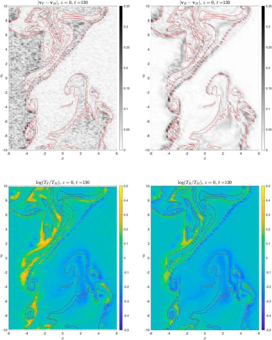
FIGURE 4. The color index represents the deviation between the bulk velocity (top) and temperature (bottom) from MHD simulation and test particles for the symmetric case at t = 130. The left and right panels show the forward tracing and backward tracing, respectively. The red lines are the contour lines of r_M = 0.5.

Figure 5 plots the logarithmic scale of the anisotropic temperature T_∥/T_⊥ (color index) at t = 0 (left) t = 130 (middle) for the symmetric case by using forward tracing method. The right panel shows the results from the backward tracing method. The black arrows represent the x and y components of the bulk velocity from MHD simulation. The magenta line represents the magnetosheath-magnetosphere boundary based on magnetic field topology. The particles were initialized isotropically (i.e., T_∥/T_⊥ = 1) at t = 0 as shown in the left panel with small fluctuations due to the statistical noise. At t = 130, anisotropic temperature regions appears around the edges of the KH vortex based on the forward tracing method, being quantitatively consistent with the results from backward tracing method, which suggests that KH instability can cause anisotropic temperature. It is interesting to note that T_∥ > T_⊥ on the magnetospheric side, while T_∥ < T_⊥ on the magnetosheath side. This can be easily explained by the DMLR process. For the newly reconnected magnetospheric closed magnetic field line, the magnetosheath-originating cold plasma (i.e., low parallel velocity) expand freely along the magnetic field line from low latitudes to high latitudes. Meanwhile, magnetosphere-originating hot plasma (i.e., high parallel velocity) expand freely along the magnetic field line from both high-latitude regions into low latitudes. Thus, on the low-latitude magnetospheric side, T_∥ becomes larger than T_⊥. Vice versa, on the magnetosheath side, the fast field-aligned expansion of the hot magnetosphere-originating plasma is replaced by the cold magnetosheath-originating plasma, which reduces T_∥. Notice, this type of anisotropic temperature generation mechanism only occurs when there is a large temperature asymmetry across the boundary, which is often satisfied at the Earth’s magnetopause boundary. It also requires a relaxing time for particles from the two sides to fully mix. One should also keep in mind, a large anisotropic temperature or even a population with a two streaming beams (field-aligned and anti-field-aligned) often leads to different types of kinetic instabilities, which eventually leads to additional nonadiabatic heating sources to bring the particle distributions to local kinetic equilibrium. These processes should also be resolved by the hybrid or PIC simulations. On the other hand, the mixing of plasma due to the finite gyroradius effect may also affect the temperature anisotropy, which is out of the scope of this study.

FIGURE 5

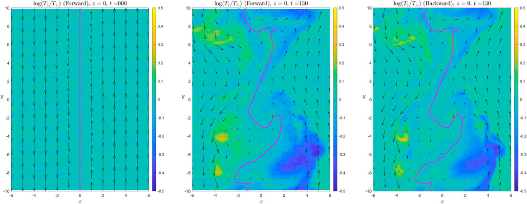
FIGURE 5. The color index represents the temperature anisotropy T_∥/T_⊥ at t = 0 (left) t = 130 (middle) for the symmetric case by using forward tracing method. The right panel shows the results from backward tracing method. The black arrows represent the x and y components of the bulk velocity from MHD simulation. The magenta line represents the magnetosheath-magnetosphere boundary based on magnetic field topology.

To systematically compare the symmetric case and the asymmetric case, we normalized the time, t, with the KH growth rate γt (Hasegawa et al., 2004; Henri et al., 2013). Here, the KH growth rate, γ, is obtained from the logarithmic fitting of t and max(δv_x) − min(δv_x) during the interval of 5 < t < 70, which gives γ = 0.0487 and 0.0439 for the symmetric and asymmetric cases, respectively. Figure 6 plots four overall parameters as functions of normalized time for the symmetric case (black lines) and the asymmetric case (red lines) for comparison. The top panel shows the range of the normal bulk velocity component to indicate the linear and nonlinear stage, which is similar to the top-right panel of Figure 2. The second panel plots the total mixed volume, V_m (i.e., similar to bottom-right panel of Figure 2), showing these two lines are almost overlapped with each other, which demonstrates that the slower mixing rate in the asymmetric case is mainly due to the slower growth rate. The third and fourth panel of Figure 6 plot the change of < |v_F − v_M| >, and < | log(T_F/T_M)| >, respectively, to illustrate the deviation of bulk velocity, and temperature between the MHD and test particle (forward tracing method) as a function of the normalized time. Here, the average <f> is weighted by the mixed rate r_M, (i.e., <f>_M = ∫fr_MdV/∫r_MdV) for mixed region (solid lines) and 1 − r_M, (i.e., <f>_N = ∫f(1 − r_M)dV/∫(1 − r_M)dV) for non-mixed region (dashed lines), and the volume integration is taken within the volume |x| < 6 and |z| < 35, covering only the KH active region. For a better comparison between the symmetric case and the asymmetric case, we also subtracted the initial value of <f>, which can be considered as background statistical noise. It clearly shows that the deviation between the MHD and test particle simulations is almost constant in the non-mixed region, while the deviation significantly increases in the mixed region during the nonlinear stage. This again suggests that within certain deviation we can use fluid simulation with test particles to investigate the early nonlinear stage of the KH instability. However, eventually, during the later nonlinear stage the feedback from particles has to be taken into account for the system, requiring hybrid or full kinetic simulations. For both bulk velocity and temperature in the mixed region, the deviation in the asymmetric case increases a bit faster than the symmetric case, which could be partially due to the preexisting magnetic shear in the asymmetric case leading to a faster onset of magnetic reconnection with kinetic effects becoming important. However, the onset of kinetic physics is somewhat arbitrary during the KH instability. For instance, in a symmetric case, fast growth of KH instability could cause secondary KH instability which leads to a thin boundary layer without involving magnetic reconnection, where gyro-radius effects can cause deviation between MHD and test particle descriptions. Meanwhile, a large magnetic shear, B_y may stabilized the KH instability, which consequently delays the onset of magnetic reconnection. Thus, to draw a general conclusion whether the test particle simulation is less applicable for the asymmetric case or not requires a much wider and systematic comparison in future studies.

FIGURE 6

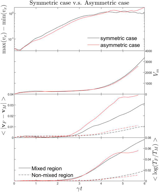
FIGURE 6. The overall dynamical properties for the symmetric case (black lines) and the asymmetric case (red lines) in a normalized time scale (i.e., γt). The top to bottom panels show the growth of the KH instability (the range of the bulk velocity v_x component), the total mixed volume, V_m (based on H+ ), the change of < |v_F − v_M| > , and change of < | log(T_F/T_M)| > for mixed region (solid lines) and non-mixed region (dashed lines).

4 Summary and Discussion

In this study, we carried out two 3-D KH instability MHD simulations accompanied by test particle simulations, in which the initial boundary condition is close to the MMS-observed KH event reported by Eriksson et al. (Eriksson et al., 2016). The simulation results suggests about 10²⁵ particles/s mass is transported from the magnetosheath into the magnetosphere via the mid-latitude-double-reconnection process, and the mixing diffusion rate is about 10¹⁰ m² s⁻¹. The presence of the magnetic B_y component reduces the KH growth rate and also strongly reduces the mass increase rate on the magnetospheric side. For Earth’s typical magnetopause boundary conditions, the finite gyroradius effect does not significantly increase the mass transport rate, even for O+. Although, a large gyroradius effect will bring a greater mixed volume, the mixing diffusion rate is insensitive to the charge-to-mass ratio in the nonlinear stage of the KH instability, partially because KH scale size is larger than gyro-radius of heavy ions (O+). However, this effect may play role in other planets (e.g., Mercury and Mars (Poh et al., 2021)). The DMLR process changes the magnetic field line topology which exchanges the low-latitude magnetic flux tubes between the magnetosheath side and the magnetosphere side. Thus, the plasma mixing can also occur through the DMLR process; however, it takes time for ion particles to undergo free expansion into the newly reconnected flux tube, which limits its effects on the mixing region.

During the KH instability process, an individual particle can be either accelerated or decelerated, however, the overall energy (subtracted by the bulk velocity) distributions do not vary with time, which indicates there is no additional heating source through this process. Although the average energy of particles moving from the magnetosheath into the magnetosphere is higher than the particles still remaining in the magnetosheath, this is simply because those transported particles were originally in a relatively higher temperature region of the initial transition layer. Thus, for the thermal particle population there is no energy filter effect for the KH instability. Nevertheless, it is still not clear whether the KH instability will select higher energy particles from the magnetosheath into the magnetosphere for the super-thermal population.

We also compared the zeroth, first, and second order moments of the particle velocity distributions from the test particle simulation with the density, bulk velocity, and temperature from the MHD simulation. It shows that the zeroth order moment is consistent with the MHD description, which also indicates the extended boundary condition along the z-direction for the test particles is consistent with the MHD boundary conditions. The first and second order moments remain consistent with the MHD bulk velocity and temperature, respectively, in the non-mixed region, but show clear deviation in the mixed region. This deviation between the particle description and the MHD description indicates that it is essential to use hybrid simulation or even PIC simulation to provide a self-consistent simulation of the later nonlinear stage of the KH instability.

Both the forward tracing method and the backward tracing method based on Liouville’s theory suggest the KH instability can generate temperature anisotropy at the edge of the KH vortex, which is also observed by the MMS [(Eriksson et al., 2016), and our companion paper (Eriksson et al., 2021)]. In this case, the anisotropic temperature is caused by the reconnection of flux tubes with two different temperatures, which is interesting to compare with the results from a double-adiabatic MHD description. This condition also brings two important questions for future study. The first one is how long does it take for particles in the newly reconnected flux tube to become fully mixed? Recall that one of the plausible magnetosheath plasma specific entropy increase mechanisms is that the magnetosheath plasma expands freely in the newly reconnected flux tube. Thus, this question is directly related to this mechanism, and a related question is whether the free expansion happens during the KH instability at the magnetopause boundary or will it take a longer time while the newly reconnected flux moves radially earth-ward? This question likely can be addressed using test particle simulations in future studies. The second question is whether additional kinetic instabilities occur during the mixing process, bringing an additional nonadiabatic heating source? This is essentially a cross-scale problem, requiring hybrid or even PIC simulation.

The results from the forward tracing and the backward tracing methods are quantitatively comparable. The backward tracing can easily increase the resolution of the velocity space for a given point, which is suitable for investigating a certain region of interest. However, one should keep in mind, this method requires the whole process be reversible. For the 3-D KH instability, the DMLR process is an irreversible process. Thus, strictly speaking, the backward tracing method is not applicable. However, the mid-latitude reconnection sites are highly localized, and no parallel electric field is present during the particle tracing. Thus, the backward tracing method still works in our study. However, in principle, it cannot be used to investigate the possible nonadiabatic heating or acceleration mechanisms.

This study also highlights the importance of using hybrid or PIC simulation to resolve the later nonlinear stage of the KH instability. However, due to the high computational cost and complex boundary conditions, only a few hybrid and PIC simulations can investigate a 3-D KH instability with a non-periodic boundary condition along the third direction and with strong temperature asymmetry across the flow layer condition. This study provides a plausible approach for the non-periodic boundary condition. Meanwhile one can use MHD and test particle simulations to simulate the linear stage and early nonlinear stage of the KH instability, and switch to the hybrid simulation when the deviation between the first or second moments from the test particle and MHD simulation is greater than a critical value, which is another plausible scenario to save on computational cost.

In summary, the KH instability is a cross-scale process, which requires a spatial resolution of both meso-scale and kinetic scale processes. Although with the development of computational hardware, hybrid simulation and PIC simulation can investigate ever increasing regimes of cross-scale physical processes, MHD simulation with test particles is still a useful tool to address many suitable questions in the KH instability, as well as provide a helpful guide for the more computationally expensive simulations.

Data Availability Statement

The simulation data and visualization tools in this paper can be accessed from https://commons.erau.edu/dm-ion-dynamics-meso-scale-3d-kelvin-helmholtz/

Author Contributions

All the simulations are done by the first author, all co-authors provided critical discussions and comments.

Funding

This research is supported from NASA grants 80NSSC18K1108, 80NSSC18K1381, and NNX17AI50G.

Conflict of Interest

The authors declare that the research was conducted in the absence of any commercial or financial relationships that could be construed as a potential conflict of interest.

Publisher’s Note

All claims expressed in this article are solely those of the authors and do not necessarily represent those of their affiliated organizations, or those of the publisher, the editors and the reviewers. Any product that may be evaluated in this article, or claim that may be made by its manufacturer, is not guaranteed or endorsed by the publisher.

Acknowledgments

We appreciate both reviewers’ helpful comments and suggestions. XM would like to thank Sheryl Nome and Ranka Lee for their encouragement during his writing.

References

Arzamasskiy, L., Kunz, M. W., Chandran, B. D. G., and Quataert, E. (2019). Hybrid-kinetic Simulations of Ion Heating in Alfvénic Turbulence. Astrophysical J. 879, 53. doi:10.3847/1538-4357/ab20cc

CrossRef Full Text | Google Scholar

Axford, W. I., and Hines, C. O. (1961). A Unifying Theory of High-Latitude Geophysical Phenomena and Geomagnetic Storms. Can. J. Phys. 39, 1433–1464. doi:10.1139/p61-172

CrossRef Full Text | Google Scholar

Birn, J. (1976). “The Resistive Tearing Mode by a Two-Dimensional Finite Difference Method,” in Computing in Plasma Physics and Astrophysics. Garching, West Germany.

Google Scholar

Birn, J., Thomsen, M. F., Borovsky, J. E., Reeves, G. D., McComas, D. J., Belian, R. D., et al. (1998). Substorm Electron Injections: Geosynchronous Observations and Test Particle Simulations. J. Geophys. Res. 103, 9235–9248. doi:10.1029/97JA02635

CrossRef Full Text | Google Scholar

Birn, J., Thomsen, M. F., Borovsky, J. E., Reeves, G. D., McComas, D. J., Belian, R. D., et al. (1997). Substorm Ion Injections: Geosynchronous Observations and Test Particle Orbits in Three-Dimensional Dynamic MHD fields. J. Geophys. Res. 102, 2325–2341. doi:10.1029/96JA03032

CrossRef Full Text | Google Scholar

Boris, J. (1970). The Acceleration Calculation from a Scalar Potential. Princeton, New Jersey: Princeton University Plasma Physics Laboratory.

Google Scholar

Burkholder, B., Delamere, P. A., Ma, X., Thomsen, M. F., Wilson, R. J., and Bagenal, F. (2017). Local Time Asymmetry of Saturn's Magnetosheath Flows. Geophys. Res. Lett. 44, 5877–5883. doi:10.1002/2017GL073031

CrossRef Full Text | Google Scholar

Burkholder, B. L., Delamere, P. A., Johnson, J. R., and Ng, C. S. (2020). Identifying Active Kelvin-Helmholtz Vortices on Saturn's Magnetopause Boundary. Geophys. Res. Lett. 47, e2019GL084206. doi:10.1029/2019GL084206

CrossRef Full Text | Google Scholar

Cerri, S. S., Arzamasskiy, L., and Kunz, M. W. (2021). On Stochastic Heating and its Phase-Space Signatures in Low-Beta Kinetic Turbulence. Astrophysical J. 916, 120. doi:10.3847/1538-4357/abfbde

CrossRef Full Text | Google Scholar

Chandran, B. D. G., Li, B., Rogers, B. N., Quataert, E., and Germaschewski, K. (2010). Perpendicular Ion Heating by Low-Frequency Alfvén-Wave Turbulence in the Solar Wind. Astrophysical J. 720, 503–515. doi:10.1088/0004-637X/720/1/503

CrossRef Full Text | Google Scholar

Chandrasekhar, S. (1961). “Hydrodynamic and Hydromagnetic Stability,” in The International Series of Monographs on Physics (New York: Dover Publ.).

Google Scholar

Cowee, M. M., Winske, D., and Gary, S. P. (2010). Hybrid Simulations of Plasma Transport by Kelvin-Helmholtz Instability at the Magnetopause: Density Variations and Magnetic Shear. J. Geophys. Res. 115, a–n. doi:10.1029/2009JA015011

CrossRef Full Text | Google Scholar

Cowee, M. M., Winske, D., and Gary, S. P. (2009). Two-dimensional Hybrid Simulations of Superdiffusion at the Magnetopause Driven by Kelvin-Helmholtz Instability. J. Geophys. Res. 114, a–n. doi:10.1029/2009JA014222

CrossRef Full Text | Google Scholar

Delamere, P. A., Ng, C. S., Damiano, P. A., Neupane, B. R., Johnson, J. R., Burkholder, B., et al. (2021). Kelvin-Helmholtz‐Related Turbulent Heating at Saturn's Magnetopause Boundary. J. Geophys. Res. Space Phys. 126, e2020JA028479. doi:10.1029/2020JA028479

CrossRef Full Text | Google Scholar

Delamere, P. A., Wilson, R. J., and Masters, A. (2011). Kelvin-Helmholtz Instability at Saturn's Magnetopause: Hybrid Simulations. J. Geophys. Res. 116, a–n. doi:10.1029/2011JA016724

CrossRef Full Text | Google Scholar

Dong, C., Wang, L., Huang, Y.-M., Comisso, L., and Bhattacharjee, A. (2018). Role of the Plasmoid Instability in Magnetohydrodynamic Turbulence. Phys. Rev. Lett. 121, 165101. doi:10.1103/PhysRevLett.121.165101

PubMed Abstract | CrossRef Full Text | Google Scholar

Eriksson, S., Lavraud, B., Wilder, F. D., Stawarz, J. E., Giles, B. L., Burch, J. L., et al. (2016). Magnetospheric Multiscale Observations of Magnetic Reconnection Associated with Kelvin-Helmholtz Waves. Geophys. Res. Lett. 43, 5606–5615. doi:10.1002/2016GL068783

CrossRef Full Text | Google Scholar

Eriksson, S., Ma, X., Burch, J. L., Otto, A., Elkington, S., and Delamere, P. A. (2021). MMS Observations of Double Mid-Latitude Reconnection Ion Beams in the Early Non-Linear Phase of the Kelvin-Helmholtz Instability. Front. Astron. Space Sci. 8, 760885. doi:10.3389/fspas.2021.760885

CrossRef Full Text | Google Scholar

Faganello, M., and Califano, F. (2017). Magnetized Kelvin-Helmholtz Instability: Theory and Simulations in the Earth's Magnetosphere Context. J. Plasma Phys. 83, 535830601. doi:10.1017/S0022377817000770

CrossRef Full Text | Google Scholar

Faganello, M., Califano, F., Pegoraro, F., Andreussi, T., and Benkadda, S. (2012). Magnetic Reconnection and Kelvin-Helmholtz Instabilities at the Earth's Magnetopause. Plasma Phys. Control Fusion 54, 124037. doi:10.1088/0741-3335/54/12/124037

CrossRef Full Text | Google Scholar

Fairfield, D. H., Otto, A., Mukai, T., Kokubun, S., Lepping, R. P., Steinberg, J. T., et al. (2000). Geotail Observations of the Kelvin-Helmholtz Instability at the Equatorial Magnetotail Boundary for Parallel Northward fields. J. Geophys. Res. 105, 21159–21173. doi:10.1029/1999JA000316

CrossRef Full Text | Google Scholar

Franci, L., Stawarz, J. E., Papini, E., Hellinger, P., Nakamura, T., Burgess, D., et al. (2020). Modeling MMS Observations at the Earth's Magnetopause with Hybrid Simulations of Alfvénic Turbulence. Astrophysical J. 898, 175. doi:10.3847/1538-4357/ab9a47

CrossRef Full Text | Google Scholar

Grošelj, D., Cerri, S. S., Bañón Navarro, A., Willmott, C., Told, D., Loureiro, N. F., et al. (2017). Fully Kinetic versus Reduced-Kinetic Modeling of Collisionless Plasma Turbulence. Astrophysical J. 847, 28. doi:10.3847/1538-4357/aa894d

CrossRef Full Text | Google Scholar

Hasegawa, H., Fujimoto, M., Phan, T.-D., Rème, H., Balogh, A., Dunlop, M. W., et al. (2004). Transport of Solar Wind into Earth's Magnetosphere through Rolled-Up Kelvin-Helmholtz Vortices. Nature 430, 755–758. doi:10.1038/nature02799

PubMed Abstract | CrossRef Full Text | Google Scholar

Henri, P., Cerri, S. S., Califano, F., Pegoraro, F., Rossi, C., Faganello, M., et al. (2013). Nonlinear Evolution of the Magnetized Kelvin-Helmholtz Instability: From Fluid to Kinetic Modeling. Phys. Plasmas 20, 102118. doi:10.1063/1.4826214

CrossRef Full Text | Google Scholar

Henry, Z. W., Nykyri, K., Moore, T. W., Dimmock, A. P., and Ma, X. (2017). On the Dawn-Dusk Asymmetry of the Kelvin-Helmholtz Instability between 2007 and 2013. J. Geophys. Res. Space Phys. 122, 11,888–11,900. doi:10.1002/2017JA024548

CrossRef Full Text | Google Scholar

Hwang, K. J., Goldstein, M. L., Kuznetsova, M. M., Wang, Y., ViñAs, A. F., and Sibeck, D. G. (2012). The First In Situ Observation of Kelvin-Helmholtz Waves at High-Latitude Magnetopause during Strongly Dawnward Interplanetary Magnetic Field Conditions. J. Geophys. Res. (Space Physics) 117, A08233. doi:10.1029/2011ja017256

CrossRef Full Text | Google Scholar

Hwang, K. J., Kuznetsova, M. M., Sahraoui, F., Goldstein, M. L., Lee, E., and Parks, G. K. (2011). Kelvin-Helmholtz Waves under Southward Interplanetary Magnetic Field. J. Geophys. Res. Space Phys. 116. doi:10.1029/2011ja016596

CrossRef Full Text | Google Scholar

Johnson, J. R., and Cheng, C. Z. (2001). Stochastic Ion Heating at the Magnetopause Due to Kinetic Alfvén Waves. Geophys. Res. Lett. 28, 4421–4424. doi:10.1029/2001gl013509

CrossRef Full Text | Google Scholar

Johnson, J. R., Wing, S., and Delamere, P. A. (2014). Kelvin Helmholtz Instability in Planetary Magnetospheres. Space Sci. Rev. 184, 1–31. doi:10.1007/s11214-014-0085-z

CrossRef Full Text | Google Scholar

Karimabadi, H., Roytershteyn, V., Wan, M., Matthaeus, W. H., Daughton, W., Wu, P., et al. (2013). Coherent Structures, Intermittent Turbulence, and Dissipation in High-Temperature Plasmas. Phys. Plasmas 20, 012303. doi:10.1063/1.4773205

CrossRef Full Text | Google Scholar

Kavosi, S., and Raeder, J. (2015). Ubiquity of Kelvin-Helmholtz Waves at Earth's Magnetopause. Nat. Commun. 6. doi:10.1038/ncomms8019

CrossRef Full Text | Google Scholar

Li, W., André, M., Khotyaintsev, Y. V., Vaivads, A., Graham, D. B., Toledo‐Redondo, S., et al. (2016). Kinetic Evidence of Magnetic Reconnection Due to Kelvin‐Helmholtz Waves. Geophys. Res. Lett. 43, 5635–5643. doi:10.1002/2016GL069192

CrossRef Full Text | Google Scholar

Ma, X., Delamere, P., Otto, A., and Burkholder, B. (2017). Plasma Transport Driven by the Three-Dimensional Kelvin-Helmholtz Instability. J. Geophys. Res. Space Phys. 122, 10,382–10,395. doi:10.1002/2017ja024394

CrossRef Full Text | Google Scholar

Ma, X., Nykyri, K., Dimmock, A., and Chu, C. (2020). Statistical Study of Solar Wind, Magnetosheath, and Magnetotail Plasma and Field Properties: 12+ Years of THEMIS Observations and MHD Simulations. J. Geophys. Res. Space Phys. 125, e2020JA028209. doi:10.1029/2020JA028209

CrossRef Full Text | Google Scholar

Ma, X., Delamere, P. A., Nykyri, K., Burkholder, B., Neupane, B., and Rice, R. C. (2019). Comparison between Fluid Simulation with Test Particles and Hybrid Simulation for the Kelvin‐Helmholtz Instability. J. Geophys. Res. Space Phys. 124, 6654–6668. doi:10.1029/2019JA026890

CrossRef Full Text | Google Scholar

Ma, X., Otto, A., and Delamere, P. A. (2014). Interaction of Magnetic Reconnection and Kelvin-Helmholtz Modes for Large Magnetic Shear: 1. Kelvin-Helmholtz Trigger. J. Geophys. Res. Space Phys. 119, 781–797. doi:10.1002/2013JA019224

CrossRef Full Text | Google Scholar

Ma, X., Otto, A., and Delamere, P. A. (2014). Interaction of Magnetic Reconnection and Kelvin-Helmholtz Modes for Large Magnetic Shear: 2. Reconnection Trigger. J. Geophys. Res. Space Phys. 119, 808–820. doi:10.1002/2013JA019225

CrossRef Full Text | Google Scholar

Ma, X., Otto, A., Delamere, P. A., and Zhang, H. (2016). Interaction between Reconnection and Kelvin-Helmholtz at the High-Latitude Magnetopause. Adv. Space Res. 58, 231–239. doi:10.1016/j.asr.2016.02.025

CrossRef Full Text | Google Scholar

Ma, X., and Otto, A. (2014). Nonadiabatic Heating in Magnetic Reconnection. J. Geophys. Res. Space Phys. 119, 5575–5588. doi:10.1002/2014JA019856

CrossRef Full Text | Google Scholar

Ma, X., Stauffer, B., Delamere, P. A., and Otto, A. (2015). Asymmetric Kelvin-Helmholtz Propagation at Saturn's Dayside Magnetopause. J. Geophys. Res. Space Phys. 120, 1867–1875. doi:10.1002/2014JA020746

CrossRef Full Text | Google Scholar

Masson, A., and Nykyri, K. (2018). Kelvin-Helmholtz Instability: Lessons Learned and Ways Forward. Space Sci. Rev. 214, 71. doi:10.1007/s11214-018-0505-6

CrossRef Full Text | Google Scholar

Matsumoto, Y., and Hoshino, M. (2006). Turbulent Mixing and Transport of Collisionless Plasmas across a Stratified Velocity Shear Layer. J. Geophys. Res. 111, A05213. doi:10.1029/2004JA010988

CrossRef Full Text | Google Scholar

Miura, A. (1984). Anomalous Transport by Magnetohydrodynamic Kelvin-Helmholtz Instabilities in the Solar Wind-Magnetosphere Interaction. J. Geophys. Res. 89, 801–818. doi:10.1029/ja089ia02p00801

CrossRef Full Text | Google Scholar

Miura, A., and Pritchett, P. L. (1982). Nonlocal Stability Analysis of the MHD Kelvin-Helmholtz Instability in a Compressible Plasma. J. Geophys. Res. 87, 7431–7444. doi:10.1029/JA087iA09p07431

CrossRef Full Text | Google Scholar

Moore, T. W., Nykyri, K., and Dimmock, A. P. (2016). Cross-scale Energy Transport in Space Plasmas. Nat. Phys. 12, 1164–1169. doi:10.1038/nphys3869

CrossRef Full Text | Google Scholar

Moore, T. W., Nykyri, K., and Dimmock, A. P. (2017). Ion‐Scale Wave Properties and Enhanced Ion Heating across the Low‐Latitude Boundary Layer during Kelvin‐Helmholtz Instability. J. Geophys. Res. Space Phys. 122, 11,128–11,153. doi:10.1002/2017JA024591

CrossRef Full Text | Google Scholar

Nakamura, T. K. M., Hasegawa, H., Daughton, W., Eriksson, S., Li, W. Y., and Nakamura, R. (2017). Turbulent Mass Transfer Caused by Vortex Induced Reconnection in Collisionless Magnetospheric Plasmas. Nat. Commun. 8, 1582. doi:10.1038/s41467-017-01579-0

PubMed Abstract | CrossRef Full Text | Google Scholar

Nakamura, T. K. M., Stawarz, J. E., Hasegawa, H., Narita, Y., Franci, L., Wilder, F. D., et al. (2020). Effects of Fluctuating Magnetic Field on the Growth of the Kelvin-Helmholtz Instability at the Earth’s Magnetopause. J. Geophys. Res. Space Phys. 125, e2019JA027515. doi:10.1029/2019JA027515

CrossRef Full Text | Google Scholar

Nakamura, T. K. M., and Fujimoto, M. (2008). Magnetic Effects on the Coalescence of Kelvin-Helmholtz Vortices. Phys. Rev. Lett. 101, 165002. doi:10.1103/physrevlett.101.165002

PubMed Abstract | CrossRef Full Text | Google Scholar

Nakamura, T. K. M., Fujimoto, M., and Otto, A. (2008). Structure of an MHD-Scale Kelvin-Helmholtz Vortex: Two-Dimensional Two-Fluid Simulations Including Finite Electron Inertial Effects. J. Geophys. Res. 113, a–n. doi:10.1029/2007JA012803

CrossRef Full Text | Google Scholar

Nykyri, K., Ma, X., Burkholder, B., Rice, R., Johnson, J. R., Kim, E. K., et al. (2021). Mms Observations of the Multiscale Wave Structures and Parallel Electron Heating in the Vicinity of the Southern Exterior Cusp. J. Geophys. Res. Space Phys. 126, e2019JA027698. doi:10.1029/2019JA027698

CrossRef Full Text | Google Scholar

Nykyri, K., Ma, X., Dimmock, A., Foullon, C., Otto, A., and Osmane, A. (2017). Influence of Velocity Fluctuations on the Kelvin-Helmholtz Instability and its Associated Mass Transport. J. Geophys. Res. Space Phys. 122, 9489–9512. doi:10.1002/2017JA024374

CrossRef Full Text | Google Scholar

Nykyri, K., Ma, X., and Johnson, J. (2021). Cross‐Scale Energy Transport in Space Plasmas. Magnetospheres Solar Syst. 7, 109–121. doi:10.1002/9781119815624.ch7

CrossRef Full Text | Google Scholar

Nykyri, K., Otto, A., Adamson, E., Kronberg, E., and Daly, P. (2012). On the Origin of High-Energy Particles in the Cusp Diamagnetic Cavity. J. Atmos. Solar-Terrestrial Phys. 87-88, 70–81. doi:10.1016/j.jastp.2011.08.012

CrossRef Full Text | Google Scholar

Nykyri, K., and Otto, A. (2004). Influence of the Hall Term on KH Instability and Reconnection inside KH Vortices. Ann. Geophys. 22, 935–949. doi:10.5194/angeo-22-935-2004

CrossRef Full Text | Google Scholar

Nykyri, K., Otto, A., Lavraud, B., Mouikis, C., Kistler, L. M., Balogh, A., et al. (2006). Cluster Observations of Reconnection Due to the Kelvin-Helmholtz Instability at the Dawnside Magnetospheric Flank. Ann. Geophys. 24, 2619–2643. doi:10.5194/angeo-24-2619-2006

CrossRef Full Text | Google Scholar

Nykyri, K., and Otto, A. (2001). Plasma Transport at the Magnetospheric Boundary Due to Reconnection in Kelvin-Helmholtz Vortices. Geophys. Res. Lett. 28, 3565–3568. doi:10.1029/2001GL013239

CrossRef Full Text | Google Scholar

Otto, A. (2006). Mass Transport at the Magnetospheric Flanks Associated with Three-Dimensional Kelvin- Helmholtz Modes. AGU Fall Meet. Abstr. 2006, SM33B–0365.

Google Scholar

Otto, A. (1990). 3d Resistive Mhd Computations of Magnetospheric Physics. Comput. Phys. Commun. 59, 185–195. doi:10.1016/0010-4655(90)90168-z

CrossRef Full Text | Google Scholar

Otto, A., and Fairfield, D. H. (2000). Kelvin-Helmholtz Instability at the Magnetotail Boundary: MHD Simulation and Comparison with Geotail Observations. J. Geophys. Res. 105, 21175–21190. doi:10.1029/1999JA000312

CrossRef Full Text | Google Scholar

Poh, G., Espley, J. R., Nykyri, K., Fowler, C. M., Ma, X., Xu, S., et al. (2021). On the Growth and Development of Non‐Linear Kelvin-Helmholtz Instability at Mars: MAVEN Observations. J. Geophys. Res. Space Phys. 126, e2021JA029224. doi:10.1029/2021JA029224

CrossRef Full Text | Google Scholar

Pu, Z.-Y., and Kivelson, M. G. (1983). Kelvin-Helmholtz Instability at the Magnetopause: Energy Flux into the Magnetosphere. J. Geophys. Res. 88, 853–861. doi:10.1029/JA088iA02p00853

CrossRef Full Text | Google Scholar

Pu, Z.-Y., and Kivelson, M. G. (1983). Kelvin:Helmholtz Instability at the Magnetopause: Solution for Compressible Plasmas. J. Geophys. Res. 88, 841–852. doi:10.1029/JA088iA02p00841

CrossRef Full Text | Google Scholar

Quataert, E. (1998). Particle Heating by Alfvenic Turbulence in Hot Accretion Flows. Astrophysical J. 500, 978–991. doi:10.1086/305770

CrossRef Full Text | Google Scholar

Settino, A., Malara, F., Pezzi, O., Onofri, M., Perrone, D., and Valentini, F. (2020). Kelvin-Helmholtz Instability at Proton Scales with an Exact Kinetic Equilibrium. Astrophysical J. 901, 17. doi:10.3847/1538-4357/abada9

CrossRef Full Text | Google Scholar

Sonnerup, B. U. Ö. (1980). Theory of the Low-Latitude Boundary Layer. J. Geophys. Res. 85, 2017–2026. doi:10.1029/ja085ia05p02017

CrossRef Full Text | Google Scholar

Stawarz, J. E., Eriksson, S., Wilder, F. D., Ergun, R. E., Schwartz, S. J., Pouquet, A., et al. (2016). Observations of Turbulence in a Kelvin-Helmholtz Event on 8 September 2015 by the Magnetospheric Multiscale mission. J. Geophys. Res. Space Phys. 121, 11,021–11,034. doi:10.1002/2016JA023458

CrossRef Full Text | Google Scholar

Terasawa, T., Fujimoto, M., Karimabadi, H., and Omidi, N. (1992). Anomalous Ion Mixing within a Kelvin-Helmholtz Vortex in a Collisionless Plasma. Phys. Rev. Lett. 68, 2778–2781. doi:10.1103/PhysRevLett.68.2778

PubMed Abstract | CrossRef Full Text | Google Scholar

Told, D., Jenko, F., TenBarge, J. M., Howes, G. G., and Hammett, G. W. (2015). Multiscale Nature of the Dissipation Range in Gyrokinetic Simulations of Alfvénic Turbulence. Phys. Rev. Lett. 115, 025003. doi:10.1103/PhysRevLett.115.025003

PubMed Abstract | CrossRef Full Text | Google Scholar

Vasquez, B. J. (2015). Heating Rate Scaling of Turbulence in the Proton Kinetic Regime. Astrophysical J. 806, 33. doi:10.1088/0004-637X/806/1/33

CrossRef Full Text | Google Scholar