Reproducibility of the Geomagnetically Induced Currents at Middle Latitudes During Space Weather Disturbances

Key Points

1. The geomagnetically induced currents in Hokkaido, Japan (35.7° GML), are correlated with B_y (cc > 0.8) for short periods (T < 1 h), while the correlation is poor (cc < 0.3) for long periods (T > 6 h).

2. The GICs with periods of 1 min to 24 h are well correlated with the electric field, E_x, induced by B_y in the semi-infinite one-layer conductivity model (cc > 0.85) and two-layer model (cc > 0.95) composed of highly conductive upper layer.

3. The strong B_y dependence of the GIC is also observed at lower latitude in Japan (25.3° GML) with cc > 0.85.

4. The B_y dependence of the midlatitude GIC may be associated with the ionosphere-ground currents transmitted by the TM₀ mode waves in the earth-ionosphere waveguide from high latitude to the equator.

Introduction

Geomagnetic disturbances have been known to induce electric fields on the surface of the Earth, which create a potential difference between transformers in the power transmission line system. The potential difference drives electric currents [geomagnetically induced currents (GICs)] in the power lines through the Earthing lines of the transformers (Pirjola, 1983). The GIC is a quasi-steady current, compared to the frequency (50 Hz or 60 Hz) of the power system, and has the larger magnitude at higher latitudes, particularly at the auroral latitudes where the auroral electrojets cause large-amplitude disturbances in the northward magnetic field ($B_x$) on the ground. The magnetic disturbances often go over 2000 nT and occasionally cause blackouts of the power system, as actually occurred in Canada and USA in March 1989 (Bolduc, 2002).

The GIC is derived from formula relating the GIC and the surface electric field; $GIC=a{E}_x\left(t\right)+b{E}_y\left(t\right)$, where $E_{x,y}$ is the surface electric field measured or calculated from the surface magnetic fields, and a and b are the parameters, which depend on the topology and the electrical characteristics of the system (Pulkkinen et al., 2007; Viljanen et al., 2012; Wei et al., 2013). The surface impedance has been widely used to estimate the electric fields from the magnetic fields through the relationship; E_x,y = Z·B_y,_x/μ, where B_y,_x, μ, and Z are the horizontal magnetic field, magnetic permeability, and surface impedance, respectively. The surface impedance is derived from the ground conductivity and layer thickness through the complex-image method (Boteler and Pirjola, 1998) and from the measured GIC and surface magnetic fields (Pulkkinen et al., 2007).

On the other hand, it was reported that the GIC is much more closely related to time derivatives (dB/dt) than B (deflection from the pre-event value) (Viljanen, 1997; Trichtchenko and Boteler, 2006) and the GIC has been evaluated by quite a few papers from dB/dt using the Faraday’s law (Viljanen, 1997; Pirjola, 2000; Carter et al., 2016; Kozyreva et al., 2018). It should be noted, on the other hand, that dB/dt is related to the spatial derivative of the electric field, E, in the Faraday’s law. No clear correspondence between the GIC and $d{B}_{x,y}/dt$ reported by Pirjola (1983) may be an example of an inappropriate application of dB/dt to the GIC. The dB/dt method has been used to assess the GIC even under the equatorial electrojet where the GIC has never been measured (Ngwira et al., 2013; Carter et al., 2016). It should be noted that the induction theory tells us that dB/dt should be convolved with the function of 1/$\sqrt{t}$ (t: time) (Cagniard, 1953; Viljanen and Pirjola, 1989) that is a response of the conductor to step function-like magnetic field changes (Cheng, 1959). Thus, the sole usage of dB/dt does not meet the induction theory except that the model is composed of two layers with less conductive upper layer over the highly conductive lower layer (Pirjola, 2010).

Watari et al. (2009) demonstrated that the middle latitude GIC in Hokkaido (35.7° GML), Japan, is not correlated with $d{B}_{x,y,z}/dt$ nor with the x-component magnetic field, $B_x$(deflection from the pre-event value), but very well correlated with the y-component magnetic field, $B_y$, with the correlation coefficients (cc) > 0.8. This result meets the two-layer model with the highly conductive upper layer (Pirjola, 2010). Concerning the strong $B_y$dependence, Watari et al. (2009) suggested that the GIC is a return current of the ionospheric currents carried by the TM₀ mode waves in the Earth-ionosphere waveguide, which was applied to explain the instantaneous transmission of the polar electric field and currents to the equator (Kikuchi et al., 1978). Brändlein et al. (2012) also suggested that the GIC is closely associated with the ionospheric currents by showing diurnal and seasonal variations of the GIC observed at low latitude in northern Chile.

The Hokkaido GIC has been reproduced from the ground magnetic fields using the surface impedance (Pulkkinen et al., 2010). Furthermore, Love and Swidinski (2015) reproduced the geoelectric field (GEF) measured at Kakioka, Japan (27.8° GML), from the magnetic fields at Kakioka using the convolution of dB/dt and the response of the semi-infinite one-dimensional flat Earth. Love and Swidinski (2014) solved the diffusion equation using the Laplace transformation and applied the function of $\sqrt{t}$ named linear ramp function for the convolution with dB/dt. The reproduced IEF was plotted in good shape with the observed GEF, but the correlation is not evaluated quantitatively.

As overviewed above, there are various methods to reproduce the GIC/GEF from the surface magnetic field such as from $B_y$, dB/dt, surface impedance and from the convolution of dB/dt and response functions. The variety of the method may be due to many factors affecting the GIC such as directions of power lines and coastlines, 3-D structures of Earth’s conductivities (Goto, 2015; Nakamura et al., 2018; Ivannikova et al., 2018), and the propagation mode that transports magnetic disturbances from the ionosphere and magnetosphere into the Earth. In this study, we revisit the GIC in Hokkaido to construct a model that reproduces the GIC from the observed magnetic field, B_y. The model is not to clarify the structure of the Earth’s conductivity that has been made by other methods like the magneto-telluric (MT) method but is rather a tool designed so as to reproduce the GIC from the surface magnetic field as accurately as possible. As a next step to the accomplishment of the good correlations between the GIC and B_y (Watari et al., 2009), we examine if the GIC-B_y correlations are valid for any space weather disturbances with different period/time scales ranging from 1 min to 24 h. As shown in the following sections, we found that the GIC-B_y correlation depends on the period of disturbances such that cc > 0.8 for short periods (<1 h) and cc < 0.3 for long periods (>6 h). To construct a model capable of reproducing the long period GIC, we calculated the IEF, $E_{x,y}$ using the convolution of $d{B}_{y,x}/dt$ and the step response of the semi-infinite one-layer conductivity model. The GIC-$E_x$ correlation is shown to be much better (cc (GIC-$E_x$) > 0.9) than cc (GIC-$B_y$) for long periods, while cc (GIC-$B_y$) is still better than cc (GIC-$E_x$) for short periods. To construct a model covering both short and long periods, we built the two-layer model composed of highly conductive upper layer over less conductive semi-infinite lower layer. The two-layer model is shown to reproduce the GIC with cc > 0.9 for periods ranging from 1 min to 24 h. In Derivation of the IEF from the Observed Magnetic field, we formulate equations that derive the IEF from the observed magnetic field in one- and two-layer models. Then, we calculate correlation coefficients of the GIC with B_x,y and E_y,x induced in the one- and two-layer models in Correlations among Observed GIC, B_x,y and E_y,x. In order to evaluate the capability of the model for various types of space weather events, we analyzed impulsive geomagnetic sudden commencement (SC), short-period (1 min) geomagnetic Pi2 pulsations, longer-period (30 min-8 hours) DP2 fluctuations, and solar quiet diurnal variations (Sq), isolated substorm magnetic bays, and long-lasting storm disturbances (1–24 h). To examine the generality of the model, we applied the model to the GIC measured at the Shin-Yamaguchi (SYG) substation of the Chugoku Electric Company located at lower latitudes in Japan (25.3° GML). We found that the model well reproduced the GIC at SYG with high correlation coefficients (cc = 0.87–0.95) for DP2 and SC events with strong B_y dependence. In Discussion, we discuss that the daytime GIC can be connected with the ionospheric currents by the TM₀ mode waves in the Earth-ionosphere waveguide, which carry the ionospheric currents from the polar ionosphere to the equator (Kikuchi et al., 1978; Kikuchi, 2014). We further stress that large-amplitude GICs tend to occur around the midnight during substorms, which raises an issue on the propagation mode from the magnetospheric currents to the ground on the nightside.

Derivation of the IEF from the Observed Magnetic field

Convolution Theorem

The magnetic field, $B_y$, propagates downward in the Earth (a conducting medium) as described by the diffusion equation derived from the Faraday’s law, Ampere’s law, and Ohm’s law. To solve the equations, we use the Laplace transformation that transforms differential equations into algebraic equations and convolution into multiplication. In the transformed equations, the time derivative is multiplication of s (s is the complex number used in the Laplace transformation), and integration is multiplication of 1/s. Following the theory of response of the linear system (Cheng, 1959), the induced electric field (IEF), $E_x\left(t\right)$, is a response of the linear system (conductor) to the external excitation (applied $B_y\left(t\right)$). Letting the Laplace transforms of $E_x\left(t\right)$ and $B_y\left(t\right)$ be $e_x\left(s\right)$ and $b_y\left(s\right)$, respectively, we express $e_x\left(s\right)$ as a product of the excitation transform, $b_y\left(s\right)$ and the transfer function,$f\left(s\right)$ (Laplace transform of the impulse response function, $F\left(t\right)$) as shown below.

$e_x\left(s\right)=f\left(s\right)\cdot b_y\left(s\right).(1)$

Here, we note that the impulse response is a response of the system to the external excitation in a form of the delta function, $\delta \left(t\right)$, of which Laplace transform is 1. The inverse Laplace transformation of Eq. 1 gives $E_x\left(t\right)$ in a form of the convolution integral of the impulse response, $F\left(t\right)$ and the external excitation, $B_y\left(t\right)$ as given by

$E_x\left(t\right)=F\left(t\right)\ast B_y\left(t\right)={\displaystyle {\int }_0^{t}F(t-\tau )B_y\left(\tau \right)}d\tau ,(2)$

where ∗ refers to the convolution of two functions. The convolution (2) implies that $E_x\left(t\right)$ is a sum of impulse responses of the system excited by $B_y$ recorded from τ = 0 to t.

We may write the Eq. 1 in a different form including 1/s (time integral) and s (time derivative) as

$e_x\left(s\right)=\left[\frac{1}{s}f\left(s\right)\right]\cdot \left[s{b}_y\left(s\right)\right].(3)$

Using Eq. 3, we can write the convolution (2) in a different form as

$E_x\left(t\right)=G\left(t\right)\ast \frac{d{B}_y\left(t\right)}{dt}={\displaystyle {\int }_0^{t}G(t-\tau )\frac{d{B}_y\left(\tau \right)}{d\tau }}d\tau +B_y\left(0\right)G\left(t\right),(4)$

where G(t) denotes the step response of the conductor, a response to the excitation function in a form of the unit step function, $U\left(t\right)$(= 1 for t > 0 and = 0 otherwise) and B_y(0) is the initial value of B_y. In the following, B_y(0) is assumed to be zero since t = 0 is set to the quiet time before the arrival of the disturbances. The convolution (4) is identical to the Eq. 12 of Cagniard (1953). It should be stressed that the IEF is obtained from dB/dt convolved with the step response of the conductor. In the following, we use Eq. 4 to derive the IEF, while Eq. 2 works the same way. Since the GIC and magnetometer data at Memambetsu (MMB), Hokkaido are sampled every one second, the time t is discrete, and the time derivative and integral in Eq. 4 are replaced with a difference and summation, respectively, as follows.

$E_x(t)={\displaystyle \sum _{i=1}^t\left(G\left[t-i\right]\left(B_y\left[i\right]-B_y\left[i-1\right]\right)\right)}\begin{array}{cc}& \end{array}(i=\mathrm{1,2,3},,,t),(5)$

where we start the summation from i = 1 since $B_y\left(t\le 0\right)=0$ is assumed.

IEF in One-Layer Model

The diffusion equation in the conductor is derived from the Faraday’s law, Ampere’s law, and Ohm’s law as listed below.

$\begin{array}{l}\nabla \times \mathit{E}=-\frac{\partial \mathit{B}}{\partial \mathit{t}}\\ \nabla \times \mathit{B}=\mu \mathit{J}\\ \mathit{J}=\sigma \mathit{E}\end{array},(6)$

where $\sigma$ and J are electric conductivity and current in the conductor, respectively.

The Eq. 6 leads to the following diffusion equations for $B_y$ and $E_x$ propagating toward the z-direction in the coordinates; x, y, and z directed toward the north, east, and down, respectively.

$\begin{array}{l}\frac{{\partial }^2{B}_y}{\partial z^2}-\mu \sigma \frac{\partial B_y}{\partial t}=0\\ \frac{\partial B_y}{\partial z}+\mu \sigma E_x=0\end{array}.(7)$

The Laplace transforms of Eq. 7 are given by

$\begin{array}{l}\frac{{\partial }^2{b}_y}{\partial z^2}-\mu \sigma s{b}_y=0\\ \frac{\partial b_y}{\partial z}+\mu \sigma e_x=0\end{array},(8)$

where the initial value of B_y is assumed to be zero as mentioned above. Transformed solutions are obtained in the following form:

$\begin{array}{l}{b}_y=a_1{e}^{-z\sqrt{\mu \sigma s}}+a_2{e}^{z\sqrt{\mu \sigma s}}\\ e_x=\frac{a_1\sqrt{s}}{\sqrt{\mu \sigma }}{e}^{-z\sqrt{\mu \sigma s}}+\frac{a_2\sqrt{s}}{\sqrt{\mu \sigma }}{e}^{z\sqrt{\mu \sigma s}}\end{array}.(9)$

We give the unit step function for $B_y\left(t\right)$ at z = 0 to obtain the step response function, which is used to derive the IEF from the convolution with $d{B}_y/dt$. The coefficients $a_{\mathrm{1,2}}$ are determined from the following boundary conditions: $B_y\left(t\right)=U\left(t\right)$ at z = 0 and $B_y\left(t\right)=0$ at $z=\infty$. We note that $B_y$ in the convolution integral (4) is the magnetic field observed at the surface of the Earth, which therefore includes effects of induced currents as well as external currents flowing in the ionosphere and magnetosphere. Whatever the source currents are, the observed $B_y$ is the boundary value for the diffusion equation in the ground.

We thus have the transformed solutions as

$\begin{array}{l}{b}_y=\frac{1}{s}{e}^{-z\sqrt{\mu \sigma s}}\\ e_x=\frac{1}{\sqrt{\mu \sigma }}\frac{1}{\sqrt{s}}{e}^{-z\sqrt{\mu \sigma s}}\end{array},(10)$

Substituting z = 0 for Eq. 10 and applying the inverse transformation, $L^{-1}\left\{1/\sqrt{s}\right\}=1/\sqrt{\pi t}$, we obtain the step response function, $G\left(t\right)$ for $E_x$ as

$G\left(t\right)=\frac{1}{\sqrt{\pi \mu \sigma }}\frac{1}{\sqrt{t}}U\left(t\right).(11)$

Substituting (11) for (5), we obtain the IEF as

$E_x\left(t\right)=\frac{1}{\sqrt{\pi \mu \sigma }}{\displaystyle \sum _{i=1}^t\left(\frac{1}{\sqrt{t-i}}U\left[t-i\right]\left(B_y\left[i\right]-B_y\left[i-1\right]\right)\right)}.(12)$

$E_y$ induced by $B_x$ is calculated by replacing $B_y$ with -$B_x$ in the Eq. 12. We calculated $E_x$ and $E_y$ with the conductivity, $\sigma ={10}^{-4}$ mho/ m, and as will be shown, the GIC is well correlated with $E_x$ (cc > 0.9) for long-period disturbances, whereas the correlation is still better with $B_y$ than with $E_x$ for short periods. This result would raise a problem that requires us to use two models to reproduce the GIC, depending on the period of disturbances. To address this problem, we construct a two-layer model as shown in the next subsection.

IEF in the Two-Layer Model

Using the earth-currents and magnetometer data, Owada (1972) showed that the subterranean electric conductivity at Memambetsu has a structure of three layers with depths of 8–20 km, 20–90 km, and 90–170 km and with conductivities higher in the top layer than in the lower layers. The MT method has revealed inhomogeneous distribution of the Earth’s conductivity in Hokkaido not only in the vertical but also in the horizontal directions (Satoh et al., 2000; Uyeshima et al., 2001; Uyeshima, 2007). However, since our purpose is to construct a model that is capable of reproducing the observed GIC, we pay our attention to the vertical profile of Owada (1972)’s results and construct a two-layer model with thickness, d = 20 km and ${\sigma }_1={10}^{-4}$mho/m in the upper layer (layer 1) over the semi-infinite less conductive (${\sigma }_2={10}^{-8}$ mho/ m) layer (layer 2). The parameter dependence of the model will be discussed in the discussion section.

We assume the magnetic field be a fixed value at z = 0 in the same way as in the one-layer model, and the magnetic permeability is common in both layers. The Laplace-transformed solutions in the layer 1 and layer 2 are given as follows:

$\begin{array}{l}{b}_{y1}=a_{11}{e}^{-z\sqrt{\mu {\sigma }_{1}s}}+a_{12}{e}^{z\sqrt{\mu {\sigma }_{1}s}}\\ e_{x1}=\frac{a_{11}\sqrt{s}}{\sqrt{\mu {\sigma }_1}}{e}^{-z\sqrt{\mu {\sigma }_{1}s}}-\frac{a_{12}\sqrt{s}}{\sqrt{\mu {\sigma }_1}}{e}^{z\sqrt{\mu {\sigma }_{1}s}}\\ b_{y2}=a_{21}{e}^{-z\sqrt{\mu {\sigma }_{2}s}}\\ e_{x2}=\frac{a_{21}\sqrt{s}}{\sqrt{\mu {\sigma }_2}}{e}^{-z\sqrt{\mu {\sigma }^{2}s}}\end{array}(13)$

We give the unit step function for $B_y$ at $z=0$ and employ the boundary conditions at $z=d$ as $b_y$ and $e_x$ being continuous across the boundary. Then, we have the following relations among the coefficients:

$\begin{array}{l}{a}_{11}+a_{12}=\frac{1}{s}\\ a_{11}{e}^{-d\sqrt{\mu {\sigma }_{1}s}}+a_{12}{e}^{d\sqrt{\mu {\sigma }_{1}s}}=a_{21}{e}^{-d\sqrt{\mu {\sigma }^{2}s}}\\ \frac{a_{11}\sqrt{s}}{\sqrt{\mu {\sigma }_1}}{e}^{-d\sqrt{\mu {\sigma }_{1}s}}-\frac{a_{12}\sqrt{s}}{\sqrt{\mu {\sigma }_1}}{e}^{d\sqrt{\mu {\sigma }_{1}s}}=\frac{a_{21}\sqrt{s}}{\sqrt{\mu {\sigma }_2}}{e}^{-d\sqrt{\mu {\sigma }_{2}s}}\end{array}(14)$

We obtain

$\begin{array}{l}{a}_{11}=\frac{1}{s}+k_{12}{\left(1-k_{12}{e}^{-2d\sqrt{\mu {\sigma }_{1}s}}\right)}^{-1}\frac{1}{s}{e}^{-2d\sqrt{\mu {\sigma }_{1}s}}\\ a_{12}=-k_{12}{\left(1-k_{12}{e}^{-2d\sqrt{\mu {\sigma }_{1}s}}\right)}^{-1}\frac{1}{s}{e}^{-2d\sqrt{\mu {\sigma }_{1}s}}\\ a_{21}=\left(1-k_{12}\left(1-e^{-2d\sqrt{\mu {\sigma }_{1}s}}\right){\left(1-k_{12}{e}^{-2d\sqrt{\mu {\sigma }_{1}s}}\right)}^{-1}\right)\frac{1}{s}{e}^{-d\sqrt{\mu s}\left(\sqrt{{\sigma }_1}-\sqrt{{\sigma }_2}\right)}\end{array}(15)$

where

$k_{12}=\frac{\left(\sqrt{{\sigma }_1}-\sqrt{{\sigma }_2}\right)}{\left(\sqrt{{\sigma }_1}+\sqrt{{\sigma }_2}\right)}(16)$

Under the condition, $\left|k_{12}{e}^{-2d\sqrt{\mu {\sigma }_{1}s}}\right|<1$ ($t\ge 1$), we can use the following series expansion that represents reflections at the boundary between the two layers.

${\left(1-k_{12}{e}^{-2d\sqrt{\mu {\sigma }_{1}s}}\right)}^{-1}=1+{\displaystyle \sum _{j=1}^n{\left(k_{12}{e}^{-2d\sqrt{\mu {\sigma }_{1}s}}\right)}^j}\begin{array}{cc}& \end{array}\left(n\to \infty \right)(17)$

where j refers to the number of reflections and n is chosen so that the summation approaches a steady value (n = 50 in the calculation below). Then, we have the coefficients as follows:

$\begin{array}{l}{a}_{11}=\frac{1}{s}{\displaystyle \sum _{j=0}^n{k}_{12}^j{e}^{-2jd\sqrt{\mu {\sigma }_1}\sqrt{s}}}\\ a_{12}=-\frac{1}{s}{\displaystyle \sum _{j=1}^n{k}_{12}^j{e}^{-2jd\sqrt{\mu {\sigma }_1}\sqrt{s}}}\\ a_{21}=\left(1-k_{12}\right)\frac{1}{s}{\displaystyle \sum _{j=0}^n{k}_{12}^j{e}^{-\left(\left(2j+1\right)d\sqrt{\mu {\sigma }_1}-d\sqrt{\mu {\sigma }_2}\right)\sqrt{s}}}\end{array}(18)$

Substituting Eq. 18 for Eq. 13, we obtain the transformed solutions as follows:

$\begin{array}{l}{b}_{y1}=\frac{1}{s}{e}^{-z\sqrt{\mu {\sigma }_1}\sqrt{s}}+{\displaystyle \sum _{j=1}^n{k}_{12}^j\left(\frac{1}{s}{e}^{-\left(2jd+z\right)\sqrt{\mu {\sigma }_1}\sqrt{s}}-\frac{1}{s}{e}^{-\left(2jd-z\right)\sqrt{\mu {\sigma }_1}\sqrt{s}}\right)}\\ e_{x1}=\frac{1}{\sqrt{\mu {\sigma }_1}}\left(\frac{1}{\sqrt{s}}{e}^{-z\sqrt{\mu {\sigma }_{1}s}}+{\displaystyle \sum _{j=1}^n{k}_{12}^j\left(\frac{1}{\sqrt{s}}{e}^{-\left(2jd+z\right)\sqrt{\mu {\sigma }_1}\sqrt{s}}+\frac{1}{\sqrt{s}}{e}^{-\left(2jd-z\right)\sqrt{\mu {\sigma }_1}\sqrt{s}}\right)}\right)\\ b_{y2}=\left(1-k_{12}\right){\displaystyle \sum _{j=0}^n{k}_{12}^j\frac{1}{s}{e}^{-\left(\left(2j+1\right)d\sqrt{\mu {\sigma }_1}+\left(z-d\right)\sqrt{\mu {\sigma }_2}\right)\sqrt{s}}}\\ e_{x2}=\left(1-k_{12}\right)\frac{1}{\sqrt{\mu {\sigma }_2}}{\displaystyle \sum _{j=0}^n{k}_{12}^j\frac{1}{\sqrt{s}}{e}^{-\left(\left(2j+1\right)d\sqrt{\mu {\sigma }_1}+\left(z-d\right)\sqrt{\mu {\sigma }_2}\right)\sqrt{s}}}\end{array}(19)$

The Laplace transform of the step response function, $g\left(s\right)$, is obtained by substituting z = 0 for $e_{x1}$ as

$g\left(s\right)=\frac{1}{\sqrt{\mu {\sigma }_1}}\left(\frac{1}{\sqrt{s}}+2{\displaystyle \sum _{j=1}^n{k}_{12}^j\frac{1}{\sqrt{s}}{e}^{-\left(2jd\right)\sqrt{\mu {\sigma }_1}\sqrt{s}}}\right)(20)$

Using the inverse Laplace transform, $L^{-1}\left\{\frac{1}{\sqrt{s}}{e}^{-\left(2jd\right)\sqrt{\mu {\sigma }_1}\sqrt{s}}\right\}=\frac{1}{\sqrt{\pi t}}{e}^{-\frac{{\left(jd\right)}^2\mu {\sigma }_1}{t}}$, we obtain the step response of the two-layer model as

$G\left[t\right]=\frac{1}{\sqrt{\pi \mu {\sigma }_1}}\frac{1}{\sqrt{t}}\left(1+2{\displaystyle \sum _{j=1}^n{k}_{12}^j{e}^{-\frac{{\left(jd\right)}^2\mu {\sigma }_1}{t}}}\right)U\left(t\right)(21)$

Using Eq. 21 in Eq. 5, we obtain the IEF from the convolution,

$E_x\left[t\right]=\frac{1}{\sqrt{\pi \mu {\sigma }_1}}\left\{{\displaystyle \sum _{i=1}^t\frac{1}{\sqrt{t-i}}\left(1+2{\displaystyle \sum _{j=1}^n{k}_{12}^j{e}^{-\frac{{\left(jd\right)}^2\mu {\sigma }_1}{t-i}}}\right)U\left[t-i\right]\left(B_y\left[i\right]-B_y\left[i-1\right]\right)}\right\}(22)$

$E_y$ induced by $B_x$ is calculated by replacing $B_y$ with -$B_x$ in the Eq. 22.

Correlations among Observed GIC, B_x,y, and E_y,x

The GIC was measured on the grounding conductor in the transformer of the 187 kV power line systems at the Memambetsu substation of Hokkaido Electric Power Co. Inc. (35.7° GML). The direction of the power line is southwestward, and the length of the line is approximately 100 km (Watari et al., 2009). The magnetometer observations were made at the Memambetsu magnetic observatory (http://www.kakioka-jma.go.jp/en/index.html) close to the GIC measurements.

Pi2 and SC (1–10 min)

To confirm the high correlation between the GIC and B_y (Watari et al., 2009), we picked out a Pi2 event with the period of 1 min recorded at Memambetsu (MMB) in the morning sector (0600 MLT) and a geomagnetic sudden commencement (SC) with the preliminary impulse (PI, 1 min) followed by the main impulse (MI, 5–10 min) in the morning sector (0630 MLT). Figure 1 shows $B_x$ and $B_y$ at MMB (top left) and the GIC (bottom left) observed during the Pi2 event. The GIC is well correlated with B_y (cc = 0.90), while almost nothing with B_x (cc = -0.21). The Pi2 often occurs on the nightside during substorms, while also observed on the dayside as the event in Figure 1 is the case (e.g., Han et al., 2004). The daytime Pi2 has been attributed to ionospheric currents flowing from the polar ionosphere to the equator carried by the TM₀ mode waves in the Earth-ionosphere waveguide (Sutcliffe and Lühr, 2010; Imajo et al., 2015). The TM₀ mode waves propagating southward (-x direction) have the magnetic field $B_y$ perpendicular to the propagation plane and the electric fields,$E_{x,z}$ in the propagation plane, which transport the ionospheric and ground surface currents with north-south direction (Kikuchi and Araki, 1979). The good correlation between the GIC and $B_y$ may indicate that the GIC is the ground surface current transported by the TM₀ mode waves as suggested by Watari et al. (2009) and Brändlein et al. (2012).

FIGURE 1

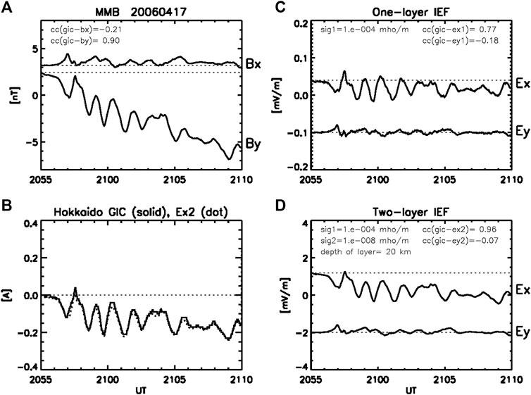
FIGURE 1. (A) X- and Y-components of the magnetic field (B_x, B_y) observed at the Memambetsu (MMB) magnetic observatory during the Pi2 event with the period of 1 min in the morning sector (21 UT, 06 MLT). (B) GIC observed at the Memambetsu substation of the Hokkaido Electric Company (solid curve). E_x2 scaled to the GIC is plotted with the dotted curve in the frame of the GIC, so that one can see the high correlation between the GIC and E_x2. (C, D) The induced electric fields (IEF), E_y,x induced by B_x,y at the surface of the Earth in the one- and two-layer models. Sig1 = 10^–4 mho/ m in the one-layer model denotes the conductivity of the semi-infinite uniform conductor. The parameters of the two-layer model are sig1 = 10^–4 mho/ m and depth = 20 km of the upper layer and sig2 = 10^–8 mho/ m of the semi-infinite lower layer. The cc refers to the correlation coefficient between the GIC and B_x,y/E_y,x.

Figure 1 also shows the IEF in one-layer model, $E_{x\text{I}}$ and $E_{\text{yI}}$ induced by $B_y$ and $B_x$, respectively (top right), and the IEF in the two-layer model, $E_{x\text{II}}$ and $E_{y\text{II}}$ (bottom right). The correlation coefficient of the GIC with $E_{x\text{I}}$ is $cc\left(GIC-E_{x\text{I}}\right)=0.77$, less than $cc\left(GIC-B_y\right)=0.90$, but the correlation with $E_{x\text{II}}$ is $cc\left(GIC-E_{x\text{II}}\right)=0.96$, indicating that the GIC can be reproduced almost perfectly by the two-layer model. $E_{x\text{II}}$ is plotted in the frame of the GIC with the dotted curve, where$E_{x\text{II}}$ is scaled to the GIC so that one can see the correlation with the GIC visually. On the other hand, the correlations with $E_{\text{yI}}$ and $E_{y\text{II}}$ are almost nothing (cc = -0.18 and -0.07) in the same way as the correlation with $B_x$, indicating that the GIC has no relations with $B_x$.

Figure 2 shows the SC event with the positive PI followed by the negative MI in $B_x$ and negative PI followed by the positive MI in $B_y$. The GIC is well correlated with $B_y$ (cc = 0.91) in the same manner as the Pi2 event. The PI and MI in $B_x$ are caused by ionospheric Hall currents driven by the dusk-to-dawn and dawn-to-dusk electric fields, respectively, while those in $B_y$ are due to north-south Pedersen currents flowing from the polar to the equatorial ionosphere (Kikuchi et al., 2001). The MI of SC in $B_x$ is primarily composed of a stepwise increase caused by the magnetopause currents, superimposed by negative deflections due to the ionospheric Hall current in the morning sector (2130 UT, 0630 MLT) (Kikuchi et al., 2001). Since the Pedersen currents of the PI and MI are transmitted by the TM₀ mode waves (Kikuchi, 2014), the GIC is consistent with being the ground surface currents carried by the TM₀ mode waves.

FIGURE 2

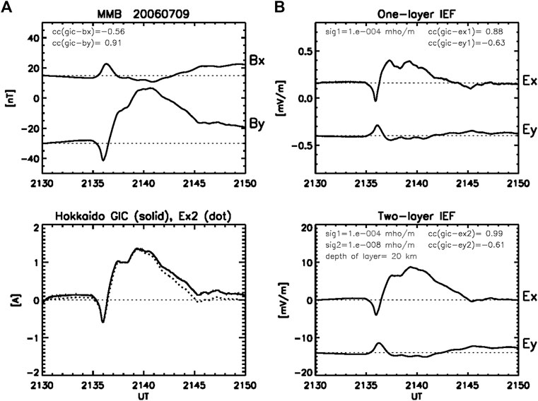
FIGURE 2. (A) B_x, B_y and GIC observed at MMB, and (B) E_x and E_y calculated in the one- and two-layer models for the SC event with time scales of 1–10 min observed in the morning sector (2130 UT, 0630 MLT). The parameters and formats of the plots are the same as in Figure 1.

Figure 2 (right panels) shows the IEF in one- and two-layer models. The correlation of the GIC with $E_{x\text{I}}$, $cc\left(GIC-E_{x\text{I}}\right)=0.88$, is less than the correlation with $B_y$, $cc\left(GIC-B_y\right)=0.91$, but the correlation with $E_{x\text{II}}$ is extremely good as $cc\left(GIC-E_{x\text{II}}\right)=0.99$. The GIC can be reproduced almost perfectly by the two-layer model as shown with the solid and dotted curves in the frame of GIC. In the following sections, we examine the correlations for longer period/time scale disturbances, ranging up to 24 h.

Quasi-Periodic DP2 Fluctuations (30 min)

Figure 3 shows periodic fluctuations with periods of 30 min in both $B_x$ and $B_y$ observed in the evening (10-12 UT, 19-21 MLT). The fluctuations are accompanied by Pi2 pulsations in the rising phase of each bay-like increase, which may imply that the fluctuations are associated with repetitive substorms (Sutcliffe and Lyons, 2002). Therefore, the fluctuations are quasi-magnetostatic field of the substorm current wedge that can be calculated using the Biot-Savart formula, although the 30-min period is shorter than the typical recurrence period (1–2 h) of substorms (Akasofu, 1964; Freeman and Morley, 2004; Borovsky and Yakymenko, 2017).

FIGURE 3

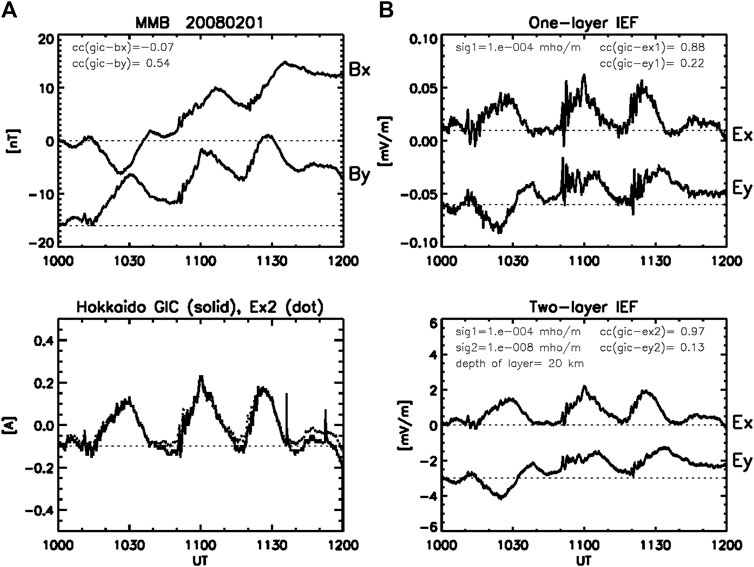
FIGURE 3. (A) B_x, B_y and GIC observed at MMB, and (B) E_x and E_y calculated in the one- and two-layer models for the DP2 fluctuation event with periods of 30 min in the evening sector (10-12 UT, 19-21 MLT). The parameters and formats of the plots are the same as in Figure 1.

The correlation of the GIC with $B_y$ is $cc\left(GIC-B_y\right)=0.54$, and the correlation with $B_x$ is almost nothing as $cc\left(GIC-B_x\right)=-0.07$. The $cc\left(GIC-B_y\right)$ is much less than the previous event, probably because the fluctuations are superimposed by the background gradual increase that may not have affected the GIC. However, the correlations with $E_{x\text{I}}$ are much better as $cc\left(GIC-E_{x\text{I}}\right)=0.88$ and almost perfect with $E_{x\text{II}}$ as $cc\left(GIC-E_{x\text{II}}\right)=0.97$. Consequently, the two-layer model well reproduces the GIC for the 30-min period fluctuations in the same way as for the Pi2 and SC.

Substorm Bays (60 min)

Figure 4 shows two successive substorm positive bays in $B_x$(top left). The first bay event occurred in the pre-midnight (1330UT, 2230MLT), and the second in the post-midnight (1630UT, 0130 MLT). The magnetic bays in $B_x$ are positive in both events, while $B_y$ is positive in the first and negative in the second events. The positive bay in $B_x$ is caused by the wedge-type field-aligned currents flowing downward in the post-midnight and upward in the pre-midnight (McPherron et al., 1973). The positive and negative bays in $B_y$ are due to the location of MMB station being close to the upward and downward FACs in the pre- and post-midnight, respectively. The GIC (bottom left) resembles the $B_y$ in both events, and their correlation, $cc\left(GIC-B_y\right)=0.67$, is better than $cc(GIC-B_x)=0.23$ in the same manner as for the short-period disturbances, while the correlation is not so good as for the SC and Pi2. In contrast, the correlation with $E_{x\text{I}}$ is much better as $cc(GIC-E_{x\text{I}})=0.94$, and furthermore, the two-layer model almost perfectly reproduces the GIC as $cc(GIC-E_{x\text{II}})=0.97$. The change in sign of the GIC across the midnight again indicates that the GIC has no association with $B_x$. The $B_y$-dependence of the nighttime bay events raises a question on the TM₀ mode wave scenario since the magnetic bays on the nightside are caused not by ionospheric currents but primarily by field-aligned currents. It remains an issue what kind of propagation mode explains the $B_y$ dependence of the GIC on the nightside.

FIGURE 4

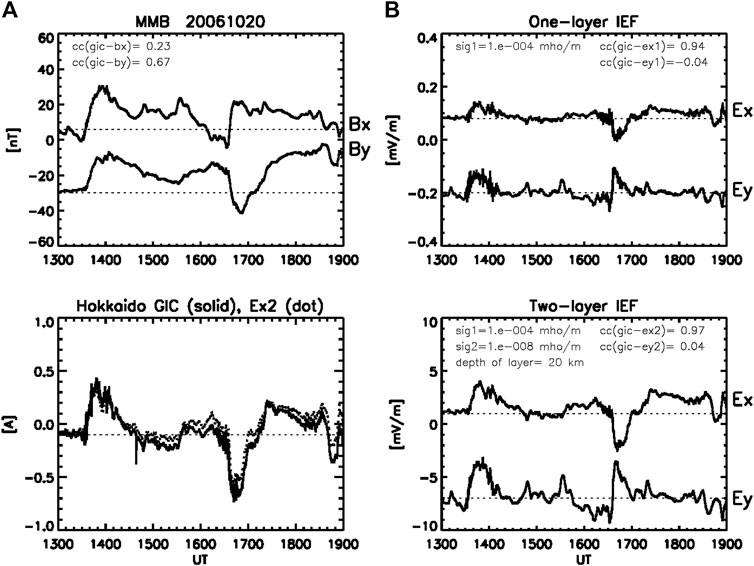
FIGURE 4. (A) B_x, B_y and GIC observed at MMB, and (B) E_x and E_y calculated in the one- and two-layer models for the substorm positive bay events with time scales of 60 min in the pre-midnight (14 UT, 23 MLT) and post-midnight (17 UT, 02 MLT). The parameters and formats of the plots are the same as in Figure 1.

Geomagnetic Storms (1–20 h)

Figure 5 shows a geomagnetic storm event, where $B_x$ shows the ring current development (00-10UT) and decay (12-18UT) superimposed by the substorm positive bay (10-11UT). The correlation of the GIC with $B_y$, $cc\left(GIC-B_y\right)=0.65$ is better than $cc\left(GIC-B_x\right)=-0.17$. The correlations with the IEF, $cc\left(GIC-E_{x\text{I}}\right)=0.92$ and $cc\left(GIC-E_{x\text{II}}\right)=0.97$ are much better than $cc\left(GIC-B_y\right)=0.65$. Thus, the two-layer model reproduces the GIC almost perfectly during the geomagnetic storm lasting over 20 h.

FIGURE 5

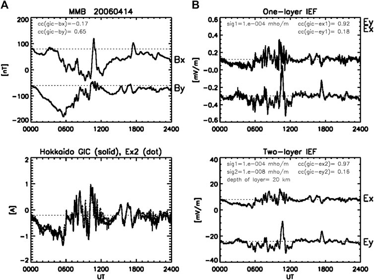
FIGURE 5. (A) B_x, B_y and GIC observed at MMB, and (B) E_x and E_y calculated in the one- and two-layer models for the geomagnetic storm events with the main phase (00-10 UT, 09-19 MLT) followed by the recovery phase (10-18 UT, 19-03 MLT) superimposed by the substorm positive bay (10-11 UT, 19-20 MLT). The parameters and formats of the plots are the same as in Figure 1.

Solar Quiet Geomagnetic Variations (8 h)

Figure 6 shows an example of the solar quiet geomagnetic variations (Sq). The period of Sq is 24 h, while significant changes occur over 8 h in the daytime (00-08 UT, 09-17 MLT). $B_x$ and $B_y$ are caused by the ionospheric currents driven by the thermospheric tidal motions (Kelley, 1989). It is remarkable that the correlation of the GIC with $B_y$, $cc\left(GIC-B_y\right)=0.27$ is much lower than those for the shorter period disturbances. Furthermore, the correlation with $B_y$ is even less than the correlation with $B_x$, $cc\left(GIC-B_x\right)=0.66$. The better correlation with $B_x$ does not necessarily mean that the GIC was caused by $B_x$, since the temporal variations of the GIC resemble those of $B_y$, if the time of $B_y$ is shifted ahead. On the other hand, the correlations with the IEF are extremely good as $cc\left(GIC-E_{x\text{I}}\right)=0.97$ and $cc\left(GIC-E_{x\text{II}}\right)=0.95$, which show close connection of the GIC with $B_y$ even under quiet conditions.

FIGURE 6

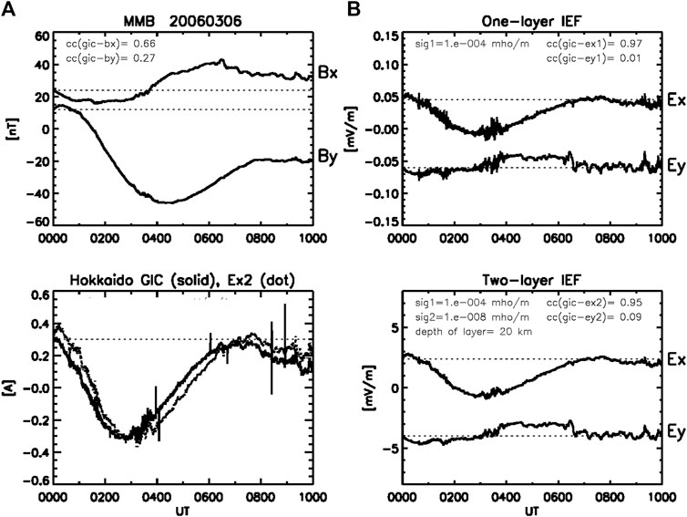
FIGURE 6. (A) B_x, B_y and GIC observed at MMB, and (B) E_x and E_y calculated in the one- and two-layer models for the solar quiet diurnal variations with time scales of 8 h (00-08 UT, 09-17 MLT). The parameters and formats of the plots are the same as in Figure 1.

Discussion

The GIC in Hokkaido, Japan, can be reproduced from $B_y$ with high correlation coefficients as shown by Watari et al. (2009). We have further shown that the reproducibility strongly depends on the period of disturbances. As summarized in Table 1, the correlation with $B_y$ is high for short periods, e.g., SC (cc = 0.91), but not for long periods, e.g., geomagnetic storm (cc = 0.65) and Sq (cc = 0.27). In particular, the correlation with $B_y$of the Sq is even lower than the correlation with $B_x$, $cc\left(GIC-B_x\right)=0.66$. Using the one-layer model composed of the semi-infinite uniform conductor with the flat surface of the ground, we have calculated the IEF, $E_x$ induced by $B_y$. The IEF is found to be highly correlated with the GIC as cc = 0.92 and 0.97 for the geomagnetic storm and Sq, respectively. This result implies that the long-period disturbances penetrated deep into the Earth, and the Earth can be considered to be uniform conductor. However, despite of the success with the one-layer model for long periods, the linear correlation with $B_y$ (cc = 0.90) is still better than that with $E_{x\text{I}}$ (cc = 0.77) for short period Pi2. This raises an issue on the period dependence of the reproducibility of the GIC.

TABLE 1

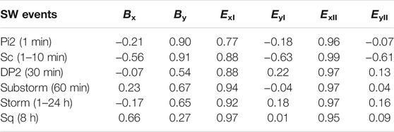
TABLE 1. Correlation coefficients between the GIC and surface magnetic fields, B_x and B_y and the electric field, E_y and E_x induced by B_x and B_y, respectively, calculated in one (I)- and two (II)-layer models for space weather (SW) events with periods ranging from 1min to 24 h.

To address this issue, we constructed the two-layer model composed of higher conductivity in the upper layer, following the previous works on the geoelectric conductivity at Memambetsu (Owada, 1972). Fujii et al. (2015), using the MT method, clarified that the apparent resistivity of the Earth increases with an increasing period of geomagnetic disturbances at Memambetsu. This result is qualitatively consistent with the two-layer model with lower conductivity in the lower layer. The two-layer model with higher conductivity in the upper layer well explains the linear relationship with B (Pirjola, 2000). As summarized in Table 1, the induced electric field in the two-layer model, $E_{x\text{II}}$, well reproduces the GIC with cc > 0.95 for both short- and long-period disturbances. To confirm the reproducibility with more events, we plotted the GIC and $E_{x\text{II}}$ for other nine events in Figure 7, where impulsive, periodic, isolated, and long-lasting disturbances on both the day and night sides are shown. The GIC (solid curve) well coincides with the $E_{x\text{II}}$ (dotted curve) that is scaled to the GIC. In particular, the peak of the GIC is well reproduced, which would help predict the GIC responsible for serious damages in the power transmission line.

FIGURE 7

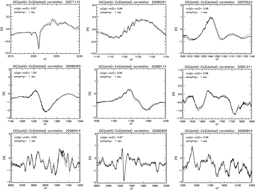
FIGURE 7. Observed GIC (solid curve) and E_x2 scaled to the GIC (dotted curve) during space weather disturbances; SC, Pi2, substorms, and storms with different time scales. The cc (gic-ex2) refers to the correlation coefficient between the GIC and E_x2, and sampling = 1 s refers to that the original 1 s sampled GIC and B_y data are used. Note that MLT = UT + 9.

We here check parameter dependence of the correlation coefficients (cc) in the two-layer model. Provided that the conductivities are fixed, major parameters responsible for cc are the number of reflections (n) and the depth of the upper layer (d₁) in the Eq. 22. Using the DP2 event in Figure 3, we calculated cc with d₁ = 20 km and different n. The cc increases as n increases such that cc = 0.94, 0.96, 0.96, 0.97, 0.97 for n = 20, 30, 40, 50, 100, respectively. We then calculated cc with fixed n = 50 and different d₁. The cc increases as d₁ increases such that cc = 0.94, 0.96, 0.97, 0.97 for d₁ = 10, 15, 20, 30 km, respectively. Thus, we fixed n = 50 and d₁ = 20 km in the two-layer model used for the calculation of the correlation coefficients.

Here, we make a brief comment on the singularity of $1/\sqrt{t}$ at t = 0 included in the step response function. Love and Swidinsky (2014), Love and Swidinsky (2015) introduced the ramp function, $\sqrt{t}$, derived from the inverse transform of $1/s\sqrt{s}$, to avoid the inconvenience in manipulating the singularity of $1/\sqrt{t}$. By using the time difference of $\sqrt{t}$, Love and Swidinsky (2015) reproduced the geoelectric field from the surface magnetic field in their two-layer model. The observed and calculated electric fields show fairly good coincidence, which may indicate success in using the ramp function. In our calculations, we replaced t with t + 0.0001 to avoid $1/\sqrt{t}=\infty$ at t = 0. This approximation worked well to achieve the excellent correlations between the IEF and GIC, while it is just technical so that 0.0001 can be replaced with another small value.

We next examine if we can estimate the GIC that could have occurred during the past major storms. For this examination, we fix scale factors, k₁ (GIC/E_x1) = 8.0 [A/(mV/m)] and k₂ (=GIC/E_x2) = 0.17 [A/(mV/m)], derived from the isolated substorm event in Figure 8. The observed GIC is well reproduced by both the one-layer and two-layer models with cc (GIC- E_x1) = 0.97 and cc (CIC- E_x2) = 0.99 as shown in the bottom left and right panels of Figure 8, respectively. For the sake of visual comparison, the observed GIC is plotted with dotted curves in each of the panels. Then, we used the scale factors, k₁ and k₂, to reproduce the GIC observed during the SC event (Figure 2). As shown in Figure 9, the GIC is well reproduced by the two-layer model with the same amplitude and high cc (=0.99), whereas the GIC is not well reproduced by the one-layer model with lower cc (= 0.88) and overestimation of the rapid changes at the onset of the SC. The good correlation between the GIC and E_x2 for the bay and SC events would allow us to use the scale factor k₂ to estimate the GIC for the past major storms. Figure 10 shows two examples of the estimated GIC during the storms on November 6, 2001 (panel (a)) and October 30, 2003 (panel (b)). It is interesting to note that the GIC estimated for the October 2003 storm has the largest magnitude at 20 UT because of the large magnitude of B_y, when the storm ring current had not fully developed yet. This result suggests strong local time dependence of the GIC at MMB, which raises an important issue from the space weather forecasting point of view.

FIGURE 8

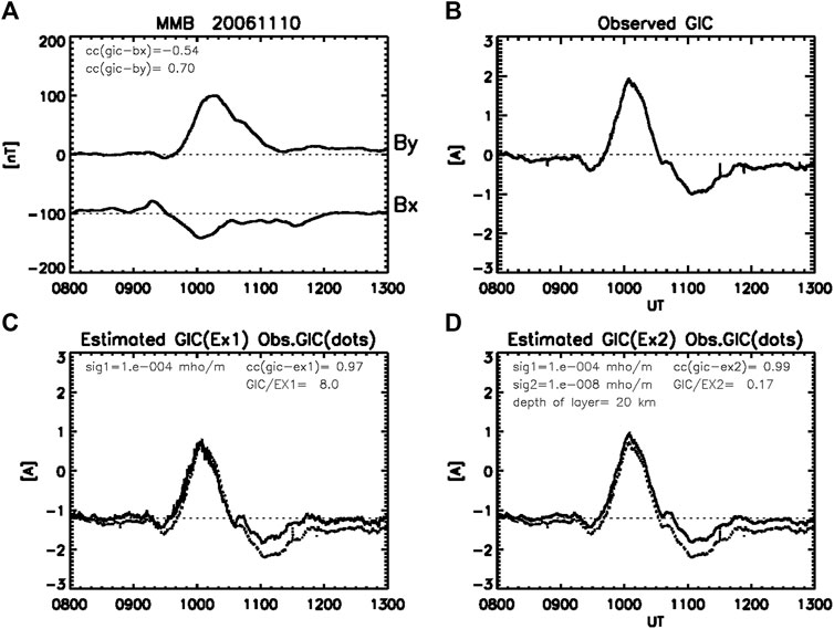
FIGURE 8. (A, B) B_x, B_y and GIC observed at MMB in the evening (10 UT, 19 MLT) during the substorm bay event. (C) GIC estimated from E_x1 scaled to the GIC with the scale factor, k₁ = 8.0 [A/(mV/m)] (solid line) and observed GIC (dotted line). (D) GIC estimated from E_x2 scaled to the GIC with the scale factor, k₂ = 0.17 [A/(mV/m)] (solid line) and observed GIC (dotted line).

FIGURE 9

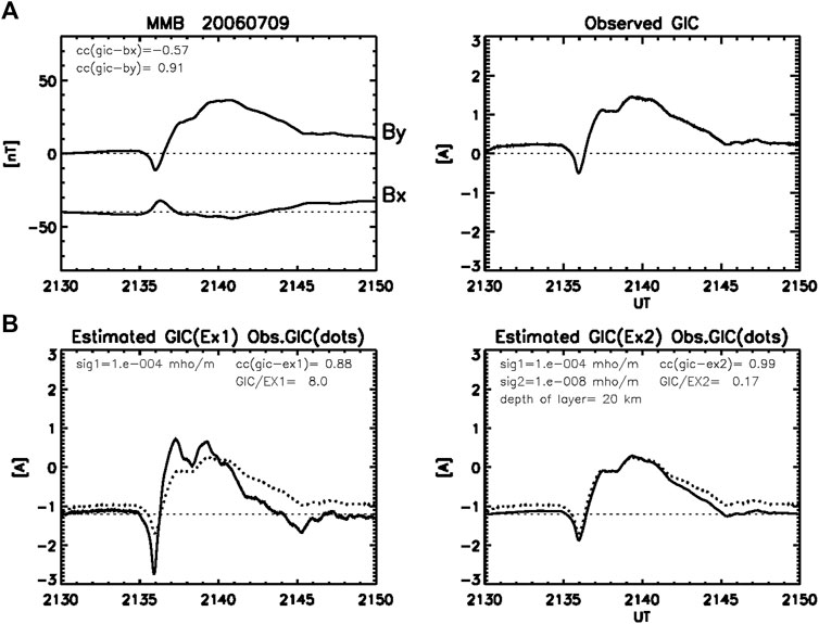
FIGURE 9. (A) B_x, B_y and GIC observed at MMB during the SC event same as in Figure 2. (B) GIC estimated from E_x1 and E_x2 scaled with the same scale factors as in Figure 8.

FIGURE 10

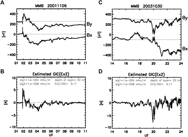
FIGURE 10. (A) Geomagnetic storms recorded at MMB in the daytime (01-09 UT, 10-18 MLT) on November 06, 2001 and (B) in the midnight-morning (16-24 UT, 01-09 MLT) on October 30, 2003. (C) (D) GICs estimated from E_x2 with the scale factor same as in Figures 8, 9.

The parameters used in the two-layer model may not represent the ones estimated by the MT method (Fujii et al., 2015), but the excellent correlations in Table 1 allow us to use the model to reproduce the GIC from the observed magnetic field disturbances. Therefore, the model should be referred to as an empirical model that works for MMB. Although the model is not a commonly applicable model, we check the model with GICs measured at the Shin-Yamaguchi (SYG) substation of the Chugoku Electric Power Company in Yamaguchi prefecture in the western-southern part of Japan (34.16°N, 131.09°E GR; 25.25°N, 201.67°E GM). The power transmission line extends in the east-west direction along the coastline. Figure 11 shows a DP2 fluctuation event (T = 80 min) observed at Kakioka (KAK, 36.23°N,140.19°E GR; 27.95°N,209.77°E GM) and the GIC at SYG, where the high frequency components are removed by applying the moving average over the window of 10 min. The KAK observatory is separated from SYG by 2.7° in GML, but the GIC is well correlated with the IEF such that cc (GIC-E_xI) = 0.85 and cc (GIC-E_xII) = 0.87. The model parameters are the same as used in the calculations for MMB except for the depth of the upper layer of the two-layer model being 15 km. Figure 12 shows an SC event with time scales of 1–10 min, where the window for the moving average is 30s. The correlation coefficients are better than those of the DP2 event such that cc (GIC-E_xI) = 0.93 and cc (GIC-E_xII) = 0.95. The correlation coefficients of the GIC with B_x/E_yII are not so good; cc = 0.54/0.14 and 0.27/0.51 for the DP2 and SC events, respectively. It is remarkable that the GIC at SYG is strongly dependent on B_y/E_x, similarly to the GIC at MMB. Furthermore, there is no big difference between the one- and two-layer models, suggesting us to use the simple one-layer model to estimate the GIC at SYG during the past major storms. Using the models constructed in the present study, we would be able to predict the GIC during space weather disturbances with the aid of the global simulations. Ebihara et al. (2014) successfully reproduced ground magnetic disturbances due to the equatorial electrojet driven by the penetration electric fields during substorms. Furthermore, Tanaka et al. (2020) reproduced magnetic disturbances due to field-aligned currents as well as the ionospheric currents during the SC and substorm.

FIGURE 11

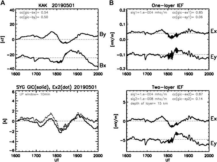
FIGURE 11. (A) B_x and B_y observed at the Kakioka (KAK) magnetic observatory and GIC observed at the Shin-Yamaguchi (SYG) substation of the Chugoku Electric Power Company during the DP2 fluctuation event with periods of 60–80 min in the early morning (16-20 UT, 01-05 MLT). The GIC data is smoothed by applying the moving average over 10 min. (B) E_x and E_y calculated in one- and two-layer models. The parameters in the frames are the same as in Figure 1 except that the depth of the upper layer of the two-layer model is 15 km.

FIGURE 12

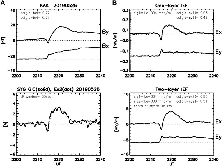
FIGURE 12. (A) B_x and B_y observed at KAK in the morning (2220 UT, 0720 MLT) and GIC at SYG during the SC event (T = 1–10 min) with the same parameters as in Figure 11, except that the GIC data is smoothed over 30s. (B) IEFs in the same format as in Figure 1.

The power transmission line in Hokkaido is directed southwestward (Watari et al., 2009), which would predict that the GIC is affected equally by both $B_x$ and $B_y$. However, as shown above, the GIC depends only on $B_y$ or $E_x$. Furthermore, the GIC depends on the B_y/E_x at SYG, where the power line and coastline are in the east-west direction. Two possible mechanisms may explain the strong $B_y$ dependence. One is that the GIC is a ground surface current induced by the TM₀ mode waves in the Earth-ionosphere waveguide (Watari et al., 2009; Brändlein et al., 2012). The TM₀ mode wave transmits the $B_y$ and $E_{x,z}$ perpendicular and parallel to the (x-z) propagation plane, respectively, carrying the ionospheric currents and ground surface currents from high latitude to the equator (Kikuchi et al., 1978; Kikuchi, 2014). The TM₀ mode propagates at the speed of light and explains the simultaneous occurrence of the PI of SC (Araki, 1977) and DP2 fluctuations (Kikuchi et al., 1996) at high latitude and equator. In Figure 13, we show the equatorial electrojet (EEJ) defined as difference in B_x between Yap, Micronesia (YAP, 0.5° GML), and Okinawa, Japan (OKI, 17.0° GML) (Kikuchi et al., 1996) together with B_x (dots) and B_y (solid) at MMB, KAK, and OKI. It is remarkable that the EEJ is well correlated with B_y at MMB, KAK, and OKI, of which amplitude decreases as the latitude decreases. The latitudinal features may indicate that the Pedersen currents responsible for B_y at middle latitudes flow into the equatorial ionosphere. Since the TM₀ mode waves induce ionospheric currents and ground surface currents (Kikuchi, 2014), it would be reasonable to attribute B_y and the GIC to the TM₀ mode waves. It should be noted, however, that the TM₀ mode wave scenario may not be valid on the nightside, since ground magnetic fields are caused by magnetospheric currents in addition to the ionospheric currents during substorms (Ritter et al., 2008). Among these currents, the field-aligned currents transport the electromagnetic energy from the magnetosphere to the polar ionosphere. Therefore, a question arises, what kind of propagation mode transports the electromagnetic energy from the foot of the field-aligned currents or directly from the magnetosphere to the power transmission line at middle latitudes on the nightside? This will be a challenging issue of the magnetosphereionosphere coupling at middle latitudes.

FIGURE 13

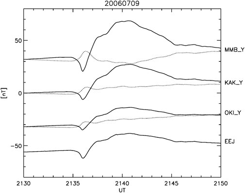
FIGURE 13. Bx (dotted lines) and By (solid lines) recorded during the SC event (Figure 2) at Memambetsu (MMB, 35.7°GML), Kakioka (KAK, 27.8°GML), Okinawa (OKI, 17.0°GML), and the magnetic deflection caused by the equatorial electrojet (EEJ) defined as the difference between Bx (YAP, 0.5°GML) and Bx (OKI). All the stations are in the same local time zone (0630 MLT).

The other possible mechanism is the effects of the geometry such as the direction of power lines and coastlines and of the 3-D structures of Earth’s conductivities (Fujii et al., 2015; Goto, 2015; Nakamura et al., 2018). Ivannikova et al. (2018) found that much of Great Britain was affected by coastal effects owing to the strong conductivity gradient between the land and the ocean. The coastline effects on the GIC are also significant in Hokkaido as deduced from the model calculations (Nakamura et al., 2018). Furthermore, Fujii et al. (2015) clarified that the MT response at Memambetsu shows that B_y affects the induction in x-direction more strongly than B_x does in y-direction. The MT-deduced anisotropy is explained by means of the spatial inhomogeneity of the Earth’s conductivity. Thus, both effects of the coastline and inhomogeneous distribution of the Earth’s conductivity should have affected the anisotropic response of the GIC to the surface magnetic field. We would need to take into account the inhomogeneous conductivity distribution even in a thin layer model (e.g., McKirdy and Weaver, 1984). However, the horizontally uniform models employed in the present study well explain the GIC-B_y/E_x correlations. The consistency between the MT and GIC results and the inconsistency between the nonuniform and uniform models remain a question to be addressed in future studies.

Conclusion

1) We have shown that the GIC at Memambetsu in Hokkaido (35.7° GML) is linearly correlated with the y-component geomagnetic field, $B_y$, for the short-period disturbances such as the geomagnetic sudden commencements (cc = 0.91) and Pi2 pulsations (cc = 0.90), while the correlation was found to become worse as the period of disturbances increases, such that cc = 0.67 for the substorm and cc = 0.27 for the solar quiet diurnal variations.

2) The induced electric field in the one-layer model with the semi-infinite conductor ($\sigma ={10}^{-4}$ mho/ m) well reproduces the GIC with cc = 0.94 for the substorm and 0.97 for the solar quiet variations. But, the correlation with $B_y$(cc = 0.91) is still better than the correlation with the induced electric field (cc = 0.88) for short period, SC.

3) We constructed the two-layer model with higher conductivity in the upper layer (${\sigma }_1={10}^{-4},{\sigma }_2={10}^{-8}$ mho/ m), which is found to be capable of reproducing the GIC with high correlations for both short periods, cc = 0.99 for SC, and for long periods, cc = 0.95 for Sq.

4) The GIC at Shin-Yamaguchi, Japan (25.3° GML) is well correlated with B_y/E_xII similarly to the GIC at MMB, such that cc = 0.87 and 0.95 for the DP2 and SC events, respectively.

5) The strong $B_y$ dependence of the GIC could be associated with the TM₀ mode in the Earth-ionosphere waveguide, which carries $B_y$ and ionosphere-ground surface currents from high latitude to the equator. This mechanism should be valid on the dayside, but it remains an issue to explain the $B_y$ dependence on the nightside, where the magnetospheric current effects dominate over the ionospheric current effects.

Data Availability Statement

The raw data supporting the conclusions of this article will be made available by the authors, without undue reservation.

Author Contributions

TK built the one- and two-layer models and wrote the whole sections of the manuscript. YE contributed to creating the GIC database and to the calculation of the IEF in the models. KKH performed space weather event studies with magnetometer data and contributed to establishing the data acquisition system from SYG substation. KK installed the GIC meter and calibrated the data at SYG. S-IW contributed to recording the GIC at MMB. All authors contributed to manuscript revision, read, and approved the submitted version.

Conflict of Interest

The authors declare that the research was conducted in the absence of any commercial or financial relationships that could be construed as a potential conflict of interest.

Publisher’s Note

All claims expressed in this article are solely those of the authors and do not necessarily represent those of their affiliated organizations, or those of the publisher, the editors and the reviewers. Any product that may be evaluated in this article, or claim that may be made by its manufacturer, is not guaranteed or endorsed by the publisher.

Acknowledgments

The measurement of the GIC at Memambetsu substation of the Hokkaido Electric Power Co., Inc., was carried out under contract with the National Institute of Information and Communications Technology (NICT) and Institute for Sun-Earth Environmental Research (ISEE), Nagoya University. This contract is subject to the data sharing restrictions defined under the Memorandum of Understanding signed by the four organizations, including the NICT (S-IW) and Nagoya University (TK). We would like to thank Mr. Yuji Watanabe, Research and Development Department, the Hokkaido Electric Power Co., Inc., for supporting the GIC measurement at Memambetsu substation. The measurement of the GIC at Shin-Yamaguchi substation of the Chugoku Electric Power Co., Inc. was carried out under contract with the National Institute of Technology/Tokuyama College (TCT) and Kibi International University (KIUI). This contract is subject to the data sharing restrictions defined under the Memorandum of Understanding signed by the three organizations, including the TCT (KK) and KIUI (K.KH). We would like to thank Mr. K. Fujii at the Chugoku Electric Power Co., Inc., for supporting the GIC measurement at the Shin-Yamaguchi substation. Those who are interested in the data may contact with any one of TK at ISEE (kikuchi@isee.nagoya-u.ac.jp), S-IW at NICT (watari@nict.go.jp), and K.KH (hashi@kiui.ac.jp). The magnetometer data at Memambetsu and Kakioka are provided by the Kakioka Magnetic Observatory of the Japan Meteorological Agency (www.kakioka-jma.go.jp). The magnetometer data at Yap and Okinawa are from the Space Weather Magnetometer Network of the NICT. This study is supported by the grants-in-aid for Scientific Research (15H05815, 20H01960) of Japan Society for the Promotion of Science (JSPS), Electric Technology Research Foundation of Chugoku, and Wesco Scientific Promotion Foundation. The works of T.K. are supported by the joint research programs of the Institute for Space-Earth Environmental Research, Nagoya University and the Research Institute for Sustainable Humanosphere, Kyoto University.

References

Akasofu, S.-I. (1964). The Development of the Auroral Substorm. Planet. Space Sci. 12, 273–282. doi:10.1016/0032-0633(64)90151-5

CrossRef Full Text | Google Scholar

Araki, T. (1977). Global Structure of Geomagnetic Sudden Commencements. Planet. Space Sci. 25, 373–384. doi:10.1016/0032-0633(77)90053-8

CrossRef Full Text | Google Scholar

Bolduc, L. (2002). GIC Observations and Studies in the Hydro-Québec Power System. J. Atmos. Solar-Terrestrial Phys. 64, 1793–1802. doi:10.1016/s1364-6826(02)00128-1

CrossRef Full Text | Google Scholar

Borovsky, J. E., and Yakymenko, K. (2017). Substorm Occurrence Rates, Substorm Recurrence Times, and Solar Wind Structure. J. Geophys. Res. Space Phys. 122, 2973–2998. doi:10.1002/2016JA023625

CrossRef Full Text | Google Scholar

Boteler, D. H., and Pirjola, R. J. (1998). The Complex-Image Method for Calculating the Magnetic and Electric fields Produced at the Surface of the Earth by the Auroral Electrojet. Geophys. J. Int. 132, 31–40.

Google Scholar

Brändlein, D., Lühr, H., and Ritter, O. (2012). Direct Penetration of the Interplanetary Electric Field to Low Geomagnetic Latitudes and its Effect on Magnetotelluric Sounding. J. Geophys. Res. 117. doi:10.1029/2012JA018008

CrossRef Full Text | Google Scholar

Cagniard, L. (1953). Basic Theory of the Magneto‐telluric Method of Geophysical Prospecting. Geophysics 18 (3), 605–635. doi:10.1190/1.1437915

CrossRef Full Text | Google Scholar

Carter, B. A., Yizengaw, E., Pradipta, R., Weygand, J. M., Piersanti, M., Pulkkinen, A., et al. (2016). Geomagnetically Induced Currents Around the World during the 17 March 2015 Storm. J. Geophys. Res. Space Phys. 121. doi:10.1002/2016JA023344

CrossRef Full Text | Google Scholar

Cheng, D. K. (1959). Analysis of Linear Systems. Addison-Wesley world student series edition.

Google Scholar

Ebihara, Y., Tanaka, T., and Kikuchi, T. (2014). Counter Equatorial Electrojet and Overshielding after Substorm Onset: Global MHD Simulation Study. J. Geophys. Res. Space Phys. 119, 7281–7296. doi:10.1002/2014JA020065

CrossRef Full Text | Google Scholar

Freeman, M. P., and Morley, S. K. (2004). A Minimal Substorm Model that Explains the Observed Statistical Distribution of Times between Substorms. Geophys. Res. Lett. 31. doi:10.1029/2004GL019989

CrossRef Full Text | Google Scholar

Fujii, I., Ookawa, T., Nagamachi, S., and Owada, T. (2015). The Characteristics of Geoelectric fields at Kakioka, Kanoya, and Memambetsu Inferred from Voltage Measurements during 2000 to 2011. Earth Planet. Sp. 67, 62. doi:10.1186/s40623-015-0241-z

CrossRef Full Text | Google Scholar

Goto, T.-n. (2015). Numerical Studies of Geomagnetically Induced Electric Field on Seafloor and Near Coastal Zones Incorporated with Heterogeneous Conductivity Distributions. Earth Planet. Sp. 67, 193. doi:10.1186/s40623-015-0356-2

CrossRef Full Text | Google Scholar

Han, D.-S., Iyemori, T., Nose, M., McCreadie, H., Gao, Y., Yang, F., et al. (2004). A Comparative Analysis of Low-Latitude Pi2 Pulsations Observed by Ørsted and Ground Stations. J. Geophys. Res. 109, A10209. doi:10.1029/2004JA010576

CrossRef Full Text | Google Scholar

Imajo, S., Yoshikawa, A., Uozumi, T., Ohtani, S., Nakamizo, A., Marshall, R., et al. (2015). Pi2 Pulsations Observed Around the Dawn Terminator. J. Geophys. Res. Space Phys. 120, 2088–2098. doi:10.1002/2013JA019691

CrossRef Full Text | Google Scholar

Ivannikova, E., Kruglyakov, M., Kuvshinov, A., Rastätter, L., and Pulkkinen, A. (2018). Regional 3-D Modeling of Ground Electromagnetic Field Due to Realistic Geomagnetic Disturbances. Space Weather. 16, 476–500. doi:10.1002/2017SW001793

CrossRef Full Text | Google Scholar

Kelley, M. (1989). The Earth’s Ionosphere, Plasma Physics and Electrodynamics. Akademic Press, Inc.

Google Scholar

Kikuchi, T., and Araki, T. (1979). Horizontal Transmission of the Polar Electric Field to the Equator. J. Atmos. Terrestrial Phys. 41, 927–936. doi:10.1016/0021-9169(79)90094-1

CrossRef Full Text | Google Scholar

Kikuchi, T., Araki, T., Maeda, H., and Maekawa, K. (1978). Transmission of Polar Electric fields to the Equator. Nature 273, 650–651. doi:10.1038/273650a0

CrossRef Full Text | Google Scholar

Kikuchi, T., Lühr, H., Kitamura, T., Saka, O., and Schlegel, K. (1996). Direct Penetration of the Polar Electric Field to the Equator during aDP2 Event as Detected by the Auroral and Equatorial Magnetometer Chains and the EISCAT Radar. J. Geophys. Res. 101, 17161–17173. doi:10.1029/96ja01299

CrossRef Full Text | Google Scholar

Kikuchi, T. (2014). Transmission Line Model for the Near-Instantaneous Transmission of the Ionospheric Electric Field and Currents to the Equator. J. Geophys. Res. Space Phys. 119, 1131–1156. doi:10.1002/2013JA019515

CrossRef Full Text | Google Scholar

Kikuchi, T., Tsunomura, S., Hashimoto, K., and Nozaki, K. (2001). Field-aligned Current Effects on Midlatitude Geomagnetic Sudden Commencements. J. Geophys. Res. 106 (15), 555. doi:10.1029/2001ja900030

CrossRef Full Text | Google Scholar

Kozyreva, O. V., Pilipenko, V. A., Belakhovsky, V. B., and Sakharov, Y. A. (2018). Ground Geomagnetic Field and GIC Response to March 17, 2015, Storm. Earth Planet. Sp. 70, 157. doi:10.1186/s40623-018-0933-2

CrossRef Full Text | Google Scholar

Love, J. J., and Swidinsky, A. (2014). Time Causal Operational Estimation of Electric fields Induced in the Earth's Lithosphere during Magnetic Storms. Geophys. Res. Lett. 41, 2266–2274. doi:10.1002/2014GL059568

CrossRef Full Text | Google Scholar

Love, J. J., and Swidinsky, A. (2015). Observatory Geoelectric fields Induced in a Two-Layer Lithosphere during Magnetic Storms. Earth Planet. Sp. 67, 58. doi:10.1186/s40623-015-0213-3

CrossRef Full Text | Google Scholar

McKirdy, D. M., and Weaver, J. T. (1984). Induction in a Thin Sheet of Variable Conductance at the Surface of a Stratified Earth -- I. Two-Dimensional Theory. Geophys. J. Int. 78, 93–103. doi:10.1111/j.1365-246x.1984.tb06473.x

CrossRef Full Text | Google Scholar

McPherron, R. L., Russell, C. T., and Aubry, M. P. (1973). Satellite Studies of Magnetospheric Substorms on August 15, 1968: 9. Phenomenological Model for Substorms. J. Geophys. Res. 78 (16), 3131–3149. doi:10.1029/ja078i016p03131

CrossRef Full Text | Google Scholar

Nakamura, S., Ebihara, Y., Fujita, S., Goto, T., Yamada, N., Watari, S., et al. (2018). Time Domain Simulation of Geomagnetically Induced Current (GIC) Flowing in 500‐kV Power Grid in Japan Including a Three‐Dimensional Ground Inhomogeneity. Space Weather. 16, 1946–1959. doi:10.1029/2018SW002004

CrossRef Full Text | Google Scholar

Ngwira, C. M., Pulkkinen, A., Wilder, F. D., and Crowley, G. (2013). Extended Study of Extreme Geoelectric Field Event Scenarios for Geomagnetically Induced Current Applications. Space Weather. 11, 121–131. doi:10.1002/swe.20021

CrossRef Full Text | Google Scholar

Owada, S. (1972). On the Subterranean Electric Conductivity Near Memambetsu Deduced by the Magneto-Telluric Method (Japanese with English Abstract). Mem. Kakioka Magn. Observatory. 14 (No.2), 77–85.

Google Scholar

Pirjola, R. (2010). Derivation of Characteristics of the Relation between Geomagnetic and Geoelectric Variation fields from the Surface Impedance for a Two-Layer Earth. Earth Planet. Sp. 62, 287–295. doi:10.5047/eps.2009.09.002

CrossRef Full Text | Google Scholar

Pirjola, R. (2000). Geomagnetically Induced Currents during Magnetic Storms. IEEE Trans. Plasma Sci. 28 (6), 1867–1873. doi:10.1109/27.902215

CrossRef Full Text | Google Scholar

Pirjola, R. (1983). Induction in Power Transmission Lines during Geomagnetic Disturbances. Space Sci. Rev. 35, 185–193. doi:10.1007/978-94-009-7063-2_14

CrossRef Full Text | Google Scholar

Pulkkinen, A., Kataoka, R., Watari, S., and Ichiki, M. (2010). Modeling Geomagnetically Induced Currents in Hokkaido, Japan. Adv. Space Res. 46, 1087–1093. doi:10.1016/j.asr.2010.05.024

CrossRef Full Text | Google Scholar

Pulkkinen, A., Pirjola, R., and Viljanen, A. (2007). Determination of Ground Conductivity and System Parameters for Optimal Modeling of Geomagnetically Induced Current Flow in Technological Systems. Earth Planet. Sp. 59, 999–1006. doi:10.1186/bf03352040

CrossRef Full Text | Google Scholar

Ritter, P., and Lühr, H. (2008). Near-Earth Magnetic Signature of Magnetospheric Substorms and an Improved Substorm Current Model. Ann. Geophys. 26, 2781–2793. Available at: www.ann-geophys.net/26/2781/2008/. doi:10.5194/angeo-26-2781-2008

CrossRef Full Text | Google Scholar

Satoh, H., Nishida, Y., Ogawa, Y., Takada, M., and Uyeshima, M. (2001). Crust and Upper Mantle Resistivity Structure in the Southwestern End of the Kuril Arc as Revealed by the Joint Analysis of Conventional MT and Network MT Data. Earth Planet. Sp 53, 829–842. doi:10.1186/BF03351680

CrossRef Full Text | Google Scholar

Sutcliffe, P. R., and Lühr, H. (2010). A Search for Dayside Geomagnetic Pi2 Pulsations in the CHAMP Low-Earth-Orbit Data. J. Geophys. Res. 115. doi:10.1029/2009JA014757

CrossRef Full Text | Google Scholar

Sutcliffe, P. R., and Lyons, L. R. (2002). Association between Quiet-Time Pi2 Pulsations, Poleward Boundary Intensifications, and Plasma Sheet Particle Fluxes. Geophys. Res. Lett. 29 (9), 7–1. doi:10.1029/2001gl014430

CrossRef Full Text | Google Scholar

Tanaka, T., Ebihara, Y., Watanabe, M., Den, M., Fujita, S., Kikuchi, T., et al. (2020). Reproduction of Ground Magnetic Variations during the SC and the Substorm from the Global Simulation and Biot‐Savart's Law. J. Geophys. Res. Space Phys. 125, e2019JA027172. doi:10.1029/2019ja027172

CrossRef Full Text | Google Scholar

Trichtchenko, L., and Boteler, D. (2006). Response of Power Systems to the Temporal Characteristics of Geomagnetic Storms. Can. Conf. Electr. Comp. Eng. doi:10.1109/CCECE.2006.277733

CrossRef Full Text | Google Scholar

Uyeshima, M. (2007). EM Monitoring of Crustal Processes Including the Use of the Network-MT Observations. Surv. Geophys. 28, 199–237. doi:10.1007/s10712-007-9023-x

CrossRef Full Text | Google Scholar

Uyeshima, M., Utada, H., and Nishida, Y. (2001). Network-magnetotelluric Method and its First Results in central and Eastern Hokkaido, NE Japan. J. Int. 146, 1–19. doi:10.1046/j.0956-540x.2001.01410.x

CrossRef Full Text | Google Scholar

Viljanen, A., and Pirjola, R. (1989). Statistics on Geomagnetically-Induced Currents in the Finnish 400kV Power System Based on Recordings of Geomagnetic Variations. J. Geomagn. Geoelec. 41, 411–420. doi:10.5636/jgg.41.411

CrossRef Full Text | Google Scholar

Viljanen, A., Pirjola, R., Wik, M., Ádám, A., Prácser, E., Sakharov, Y., et al. (2012). Continental Scale Modelling of Geomagnetically Induced Currents. J. Space Weather Space Clim. 2, A17. doi:10.1051/swsc/2012017

CrossRef Full Text | Google Scholar

Viljanen, A. (1997). The Relation between Geomagnetic Variations and Their Time Derivatives and Implications for Estimation of Induction Risks. Geophys. Res. Lett. 24, 631–634. doi:10.1029/97gl00538

CrossRef Full Text | Google Scholar

Watari, S., Kunitake, M., Kitamura, K., Hori, T., Kikuchi, T., Shiokawa, K., et al. (2009). Measurements of Geomagnetically Induced Current in a Power Grid in Hokkaido, Japan. Space Weather 7. doi:10.1029/2008SW000417

CrossRef Full Text | Google Scholar

Wei, L. H., Homeier, N., and Gannon, J. L. (2013). Surface Electric fields for North America during Historical Geomagnetic Storms. Space Weather 11, 451–462. doi:10.1002/swe.20073

CrossRef Full Text | Google Scholar