Predicting Asteroid Types: Importance of Individual and Combined Features

1 Introduction

Up-to-date taxonomies and spectra are the most important tools to constrain the composition and surface mineralogy of asteroids with various methods. Those typically rely on various modeling techniques and underlying comparison with laboratory spectral measurements of meteorite samples and/or samples returned from space missions (Reddy et al., 2015). So far, this allowed for the identification of several meteorite parent bodies, for example, the howardite–eucrite–diogenite (HED) meteorites and asteroid (4) Vesta (or more broadly V-types) (McCord et al., 1970), LL chondrites, the S-type asteroids (Itokawa or Eros) (Wetherill et al., 1988; Nakamura et al., 2011) or the F-type asteroids, and the ureilite meteorites (thanks to the observed fall of the 2008 TC3 asteroid, which impacted the Earth in 2008 (Jenniskens et al., 2010). However, there are still multiple challenges linking asteroids types with meteorites and estimating their geochemical composition from remote observations. For a full review, we refer the reader to Reddy et al. (2015).

Asteroid taxonomic schemes are tied up to the type and wavelength coverage of data used for their classification as well as the number of objects studied. Early classifications were based on color, albedo, and spectral shape (Chapman et al., 1975). Those divided asteroids into three basic categories: C-carbonaceous, S-siliceous, and the U-unknown class, that is, objects that did not fit the two previous categories. Later taxonomies included an extended number of objects and features used in the classification. Several taxonomies became popular over the years; those include the Tholen taxonomy based on the Eight-Color Asteroid Survey (ECAS) survey and albedos (Tholen, 1989), the S3OS2 classification which used visible spectra obtained at the 1.52-m telescope at ESO (La Silla), or the Buss taxonomy based on the Small Main-Belt Asteroid Spectroscopic Survey (SMASS) observations in visible wavelengths (Bus and Binzel, 2002). The current Bus–DeMeo asteroid taxonomy has used the principal component analysis (PCA) of 371 asteroid spectra obtained in the visible (VIS) and near-infrared (NIR) ranges, that is, from 0.45 to 2.45 μm (DeMeo et al., 2009). The system presented 24 classes and provided an extension to an earlier taxonomy based on VIS spectra only (Bus, 1999). An additional Xn class was later added by Binzel et al. (2019). That system helped explain the compositional distribution of the asteroid main-belt and the delivery efficiency of various taxonomic types to the near-Earth asteroid population (DeMeo and Carry, 2014; Carry et al., 2016; Barucci et al., 2017; Binzel et al., 2019; Devogèle et al., 2019). Laboratory work and asteroid observations later identified space weathering processes that cause the transformation from S though Sq to Q-types in that taxonomic system (Strazzulla et al., 2005; Vernazza et al., 2009a).

Recently, neural networks have been used in the literature to perform asteroid classification. The study by Penttilä et al. (2021) presents the results of training an artificial neural network for the needs of the Gaia mission. The data used for this task were obtained from the spectra of 586 objects from DeMeo et al. (2009) and Binzel et al. (2019) in the range of 0.45 and 1.05 μm, spanned across 11 taxonomic types (A, B, C, D, K, L, Q, S, T, V, and X). Original types assigned by DeMeo et al. (2009) were processed, such that a few subclasses were generalized into their main equivalents (i.e., assigning S to types such as Sa and Sq). The data were enhanced with additional synthetic samples formed by using the principal component analysis. This study reports 86% unbalanced prediction accuracy for the task of taxonomic type prediction but cannot be directly compared to this study as it operates on slightly different data (more objects with different types assigned), a different feature set, and a different evaluation procedure. Furthermore, this study assesses the performance of the model on the selected wavelength range but does not quantify the importance of individual features.

The Bus–DeMeo taxonomy relies on spectroscopic measurements which are challenging to obtain for a large number of objects in a reasonable amount of time. Therefore, multi-filter photometry obtained in large sky surveys is often used to assign the taxonomic type to asteroids and perform compositional and evolutionary studies (e.g., Zellner et al. (1985); Carvano et al. (2010); Gil-Hutton and Licandro (2010); Sykes et al. (2000) and others).

Furthermore, surveys typically produce enormous amounts of data but can only cover a limited number of bands. For example, the Gaia mission was expected to provide spectra for about 100 000 objects in the spectral range from 0.325 to 1.1 μm (Mignard et al., 2007). The Large Synoptic Survey of the Vera Rubin Observatory is expected to provide observations in the ugrizy bandpasses for hundredths of thousands of near-Earth objects and millions of main-belt asteroids (Jones et al., 2015), and the Euclid mission will provide (visible (a broad g-r-i), Y, J, and H photometry for about 150 000 asteroids (Carry, 2018). Sergeyev et al. (2021) extracted visible colors for about ∼ 10⁵ asteroids. Those vast amounts of data require the use of fast and reliable machine learning approaches to classify those objects and link them to the current taxonomies. Furthermore, the robustness of different classification methods may have implications to the derived taxonomic distributions across the solar system, and thus its formation and evolution theories. Various studies have already performed the scientific analysis of different “big data” sets.

For example, Sykes et al. (2000) studied the distribution of color indices of asteroids and comets observed in the course of the Two Micron All Sky Survey (2MASS) and derived an approximate compositional map of the asteroid belt. Later, based on Sloan Digital Sky Survey (SDSS) data, Carvano et al. (2010) created a taxonomic classification compatible with Bus taxonomy and studied the distribution of different asteroid types in the solar system. A more detailed in-depth analysis of the SDSS data was later performed by DeMeo and Carry (2014) who also discussed the constraints on the formation and evolution of the solar system arising from the derived compositional distribution of asteroids. Popescu et al. (2016, 2018) assigned taxonomic classifications to objects observed in the course of VISTA-VHS survey and found multiple V- and A-type candidates, which are crucial in the context of the missing mantle problem (i.e., lack of basaltic mantle material as compared to iron core material present among meteorites, e.g., Burbine et al. (1996); Scott et al. (2010). Other studies focused on searching for specific taxonomic types using multi-filter data. Licandro et al. (2017) analyzed the MOVIS-C catalog to identify the V-type asteroids using infrared colors (Y-J) and (J-Ks). Similar studies were also performed based on the SDSS magnitudes, such as Solontoi et al. (2012); Roig and Gil-Hutton (2006); Oszkiewicz et al. (2014). DeMeo et al. (2019) investigated A-type candidates extracted from the SDSS catalog. Spectrophotometric characterization is also often used to constrain the composition of near-Earth objects Mommert et al. (2016); Navarro-Meza et al. (2019); Erasmus et al. (2017); Harris and Davies (1999); Bolin et al. (2020); De León et al. (2010). DeMeo et al. (2014) discussed the distribution of very red D-type asteroids located in the main belt (typically found among Jupiter trojans and in the outer main belt) and their potential origins. Thus, classification tools are essential in understanding asteroid composition and revealing multiple processes and more generally the evolution of the solar system.

These studies could benefit from data and observations made in filters that correspond to spectral features that best predict common taxonomic types. Current large surveys are an important source of information on asteroid composition and thus help understand various mechanisms and the overall formation and evolution of the solar system. However, most of those large surveys are dedicated to other astronomical objects and asteroids are only serendipitous objects. There has not yet been a large survey strictly dedicated to studying asteroids. Therefore, the optical setups of surveys are not optimized to taxonomically characterize asteroids. Furthermore, the large surveys are typically limited in the number of bands covered; thus, selecting those that improve the link to asteroid taxonomy can maximize the science output for solar system science. In this study, we investigate which spectral features provide the most information in the context of the Bus–DeMeo taxonomy, that is, which features should be observed to optimize future multi-filter surveys toward asteroid compositional studies. We also investigated various classification methods to verify their predictability of complexes and individual classes.

In section 2, we discuss the data, while section 3 describes parameterization and methodology used. In section 4, we present our results, and in section 5, we provide extended discussion. Conclusions are in section 6.

2 Data

The dataset of asteroids used in the study consists of 371 objects included in Bus–DeMeo taxonomy (DeMeo et al., 2009) as well as 195 additional objects from Binzel et al. (2019). Most of the near-infrared data were collected at the NASA IRTF with the Spex instrument in its low-resolution (R ∼150) prism mode, and a majority of the visible wavelength data is from the Small Main-Belt Asteroid Spectroscopic Survey (R ∼100) Bus and Binzel (2002). For detailed information on that data, we refer the reader to the original studies. Each object is described by a set of visible and near-infrared spectral measurements (in the range of 0.45–2.45 μm), from which a set of spectral features is calculated, which is then used as an input for classification. Each object is also assigned to one of the 24 classes (taxonomic types) as defined in the study by DeMeo et al. (2009). For the purpose of this study, the dataset was limited to only contain the taxonomic types represented by more than 10 objects, reducing the data size from 566 to 504 objects split into 12 taxonomic types (S, Sq, Sr, C, Ch, X, Xk, L, V, D, K, and Q), as presented in Table 1. This was done in order to remove severely underrepresented taxonomic types with very few objects, for which machine learning methods, based on the statistical properties of the data, are not expected to work.

TABLE 1

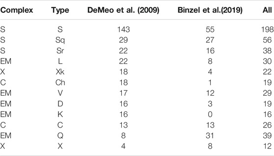
TABLE 1. Number of objects for each taxonomic type used for classification per data source.

There were two prediction tasks considered in the scope of this study: the prediction of twelve taxonomic types and simplified version of the classification, with four complexes as target (C-complex, S-complex, X-complex, and end members). The labels for the prediction of complexes were assigned based on what the taxonomic type of each asteroid belonged to, as described in DeMeo et al. (2009).

The distribution of objects in two-dimensional space (resulting from taking the two main principal components of the spectra) with respect to taxonomic types is presented in Figure 1. The preparation of feature sets obtained from the spectral data is described in detail in the following sections.

FIGURE 1

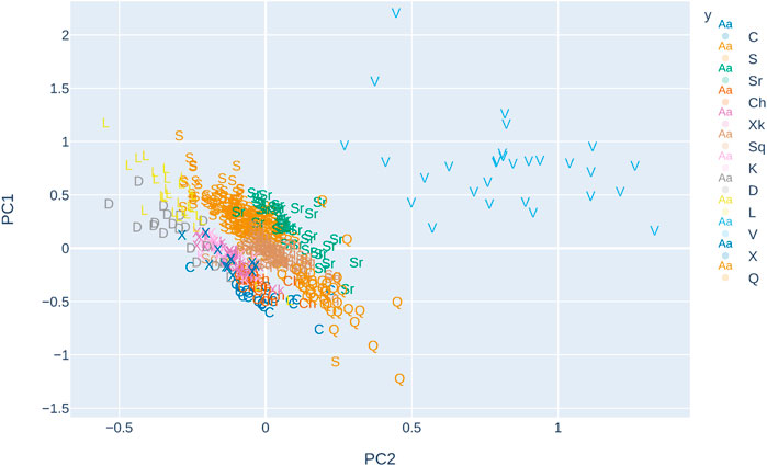
FIGURE 1. Plot represents the two main principal components of the spectra, the letters denote taxonomic types, and colors denote the complexes.

2.1 Basic Spectral Features

To obtain features based on the 0.45–2.45 μm spectral range, the input spectral measurements were processed similarly to DeMeo et al. (2009). For each object in the dataset, the first interp1d function with default parameters from SciPy library (Virtanen et al., 2020) was used to perform a linear spline fit on the spectral measurements, which generated a spectral curve. Different degrees of the spline function were selected as the input data contain enough observations that the linear fit did not result in higher inaccuracies but, at the same time, was able to extrapolate better than the cubic spline when the spectrum was not available in the desired range. We noted that this data fitting reduces the risk that the noise influenced the prediction as we do not sample the noise but the overall spectral “averaged” shape. This curve was then sampled in the range of 0.45–2.45 μm with 0.05 intervals, resulting in 41 data points. These points were normalized to unit at 0.55 μm (i.e., each point was divided by the value of the point at 0.55 μm). The feature at 0.55 μm was removed after this operation. Finally, the slope was removed from the (normalized) data points, which was performed by fitting a linear regression model to the data and dividing each data point by the value returned by the model for this point. The removal of the slope and normalization of the spectra leads to increasing visibility of other spectral features. It is worth adding that Marsset et al. (2020) found an overall 2.8% μm⁻¹ uncertainty of slope induced by the use of different solar analogs. This resulted in the set of 40 spectral features and one additional feature containing the slope of the linear regression fit for each object. The example of this processing is presented in Figure 2.

FIGURE 2

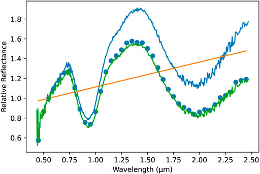
FIGURE 2. Plot represents the spectrum before processing (blue line), the fitted slope (orange line), spectrum after processing (green line), and final points (blue dots) for asteroid (1929) Kollaa.

2.2 Principal Components

The second feature set was generated by performing the principal component analysis (Jolliffe (2002) on the spectral feature set described in the previous section. PCA transforms high-dimensional feature vectors into a lower dimensional space of uncorrelated features while keeping as much of the input variance as possible, therefore retaining patterns and trends occurring in the data. Following the methodology in DeMeo et al. (2009), we first centered the 40 spectral features by subtracting from feature values their mean values calculated over the entire dataset. Then the eigenvectors and eigenvalues of the covariance matrix were calculated. The principal eigenvectors (associated with the largest eigenvalues) were selected and were used to transform the data into a new feature space. As in DeMeo et al. (2009), we selected the top five eigenvectors as a new feature set. The slope was also added as a separate feature.

3 Methodology

For all methods mentioned in this section, except for gradient boosting, the implementations from scikit-learn (Pedregosa et al., 2011) package were used.

3.1 Classification Methods

Multinomial logistic regression (Bishop, 2006) is a method that models the probability of a sample belonging to each class by constructing a linear function based on input data and applying softmax to obtain the probabilities. Specifically, the probability of class i given sample (feature vector) x is modeled as follows:

$p\left(i|\mathit{x}\right)=\frac{e^{\mathit{x}\cdot {\mathit{w}}_i}}{{\sum }_{j=1}^k{e}^{\mathit{x}\cdot {\mathit{w}}_j}},$

where ${\{{\mathit{w}}_j\}}_{j=1}^k$ are weight vectors for each class. These vectors are trained during the learning stage by minimizing the cross-entropy between the empirical class label distribution and the model distribution. The multinomial logistic regression is a relatively simple yet effective method for modeling the data, very well-studied and popular among statisticians, so it was a natural choice of the algorithm to be included in our experiment.

Naive Bayes (Hastie et al., 2009) is an algorithm that uses the Bayes theorem to calculate the conditional probability of a class given the sample p (i|x) from the prior probabilities for each class p (i) and the class-conditional probabilities of the feature vector p (x|i). The latter probabilities are estimated using a strong assumption of conditional independence between the features given the class label. In our case, the distribution of features is modeled by a Gaussian. Due to these strong modeling assumptions, naive Bayes may lack the flexibility for modeling more complex datasets but is included in the comparison as it is the arguably most popular machine learning method and proved to be surprisingly effective in various scenarios. Naive Bayes was previously applied to asteroid classification by Oszkiewicz et al. (2014) to identify V-type asteroids.

Support vector machines (SVM) (Hastie et al., 2009) perform linear classification by dividing the feature space with hyperplanes into regions such that each region corresponds to a single class. The hyperplanes are obtained in the training phase by maximizing the margin on the data, which is the distance from the nearest sample to the hyperplane. Thus, the chosen hyperplanes are those which represent the largest separation between the classes, which makes the resulting classifier robust. The main advantage of the SVM is their ability to efficiently perform a non-linear classification by an implicit mapping of the original feature vectors into a high-dimensional feature space (using the so called kernel trick), in which the data are likely to be linearly separable and thus amenable to modeling by a linear classifier. In the study, we employed the radial basis function (RBF) kernel, which provides the expressive power and flexibility of the resulting classifier sufficient for modeling even very complex datasets.

Gradient boosting (Hastie et al., 2009) is an ensemble learning method which combines multiple weak learners (relatively simple base classifiers) into a powerful classification method. The learners are added one by one to the ensemble by minimizing the gradient of the loss function (cross-entropy in this case) so that each new learner improves the performance of the previous model, effectively focusing on the samples which were previously misclassified. We employed a standard choice of the weak learner which is a decision tree with limited depth. We used the implementation of the gradient boosting provided by XGBoost (Chen and Guestrin, 2016) library due to its excellent computational performance and a comprehensive set of tunable parameters.

Multilayer perceptron (MLP) (Goodfellow et al., 2016) is a fully connected network consisting of neurons, organized into layers. The neurons produce a linear combination of the input that is passed to a non-linear activation function, in our case being the rectified linear unit. This allows us to model more complex functions and better fit the training data. We experimented with different network architectures between two and three hidden layers containing 32 or 64 neurons. We used the standard choice of the cross-entropy loss for optimization in the training phase. The network has been trained using either the stochastic gradient descent (Ruder, 2016) or Adam (Kingma and Ba, 2014) optimization methods.

3.2 Feature Selection

To evaluate the importance of individual spectral features for classification of taxonomic types, we decided to verify whether a successful classification can be achieved using only a small subset of these features. To this end, we employed the sequential forward feature selection method (Whitney, 1971). This procedure iteratively composes a feature subset by analyzing the contribution of each feature to the performance of a given machine learning model. The procedure starts with an empty set of features. At each iteration, every feature not yet included in the selected subset is, one by one, tentatively added to the subset in order to train and evaluate the model on such extended subset of features. A feature that yields the highest increase in the prediction performance is then permanently added to the selected subset, and the next iteration follows. This process is continued up to the point at which the chosen maximal size of the feature set is reached (set to 20 in the experiment). The training and evaluation of the machine learning model in each trial is performed by cross-validation. The whole process is computationally intensive as in each iteration, it requires to train and evaluate as many models as there are candidate (not yet selected) features.

3.3 Evaluation Metrics

As an evaluation metric to compare the models, we used the prediction accuracy, defined as follows:

$\text{Acc}=\sum _{i=1}\frac{T{P}_i}{N},$

where N is the total number of samples and TP_i is the number of correctly classified objects (“true positives”) from class i. Moreover, we are also reporting two additional evaluation metrics, which are known to be more robust against class imbalance (i.e., when some of the classes are much less represented in the data set than the others): the balanced prediction accuracy (BAcc) and the F₁ measure Kelleher et al. (2015)as follows:

$\begin{array}{ll}\hfill \text{BAcc}& =\frac{1}{K}\sum _{i=1}^K\frac{T{P}_i}{T{P}_i+F{N}_i},\hfill \\ \hfill F_1& =\frac{1}{K}\sum _{i=1}^K\frac{T{P}_i}{T{P}_i+\frac{1}{2}\left(F{P}_i+F{N}_i\right)},\hfill \end{array}$

where K is the total number of classes, while FP_i and FN_i are, respectively, the number of objects incorrectly classified to class i (“false positive”) and the number of incorrectly classified objects from class i (“false negatives”). The balanced prediction accuracy is thus the average recall obtained on each class, while the F₁ score is the average harmonic mean of recall and precision for each class.

Last, the Matthews correlation coefficient is reported due to better performance on imbalanced problems as opposed to other balanced metrics:

$\text{MCC}=\frac{c\times s-{\sum }_k^K{p}_k\times t_k}{\sqrt{\left(s^2-{\sum }_k^K{p}_k^2\right)\times \left(s^2-{\sum }_k^K{t}_k^2\right)}},$

where $t_k={\sum }_i^K{C}_{ik}$, the number of times class k truly occurred; $p_k={\sum }_i^K{C}_{ki}$, the number of times class k was predicted; $c={\sum }_k^K{C}_{kk}$, the total number of samples correctly predicted; and $s={\sum }_i^K{C}_{ij}$, the total number of samples and K is the total number of classes.

3.4 Experimental Setup

For both feature sets (basic spectral features and PCA features), each machine learning method, two tasks (prediction of complexes and prediction of types) and a 5-fold cross-validation procedure were performed in order to train and evaluate the model. An implementation of k-fold cross-validation from scikit-learn library (Pedregosa et al., 2011) was used. This procedure was repeated 10 times (for each combination of feature set and learning method) and averaged, to decrease the variability of the result due to a random component in the train/test split, and thus improving the reliability of the outcomes. This also allowed us to report the standard deviations of the results together with their averages.

Each of the methods used in the study has external parameters (called “hyperparameters” in machine learning), which are not optimized during the training phase but which might potentially significantly affect the prediction performance. These parameters are often tuned by an internal train-and-validate process; the training fold from cross-validation is further split into the training and evaluation parts, and a classifier is repeatedly trained and evaluated for each considered combination of parameters. The combination that leads to the best prediction performance is then selected to retrain the final classifier on the entire training fold, and its performance is then evaluated on the test fold. Balanced accuracy was selected as a measure of validating the prediction performance. The selection of aforementioned balanced metric was made based on its straightforward interpretability and ease of score understanding, while effectively compensating for the imbalance in data.

Note that for each combination of parameters, one needs to train and validate a given model 50 times, once for each fold in the fivefold cross-validation repeated 10 times, and this must be done for every learning method, and every set of features. Thus, the entire procedure is computationally very demanding; hence, the parameter tuning was limited to up to 10 tested parameter combinations per learning method.

Different parameter combinations were considered for each model. Multinomial logistic regression parameters consisted of inverse regularization strengths in the range between 5 and 60, as well as the choice of the L₁ or L₂ norm for the regularization term. Naive Bayes was examined with different variance smoothing parameters in the range (1e—10‥1e − 6), which control the portion of the largest variance of all features that is added to variances for calculation stability. Support vector machines were tested for the regularization parameter between 5 and 24 and with two choices of the kernel function: linear and RBF (with the RBF kernel parameter set to either “automatic” or “scaled”). For the gradient boosting method, the number of estimators ranged from 50 to 500, with the maximum tree depth of 3–15, learning rate between 0.01 and 0.1, and subsampling parameter being 0.75 or 1. Last, multilayer perceptron architectures consisted of 2–3 hidden layers with 32 or 64 neurons each, with the batch size of 32 or 64, the selection of stochastic gradient descent or Adam solver, and initial learning rate in the range or 0.001 to 0.1.

Sequential feature selection was performed with an implementation from the scikit-learn library (Pedregosa et al., 2011) on the task of predicting taxonomic types. As this process is already computationally extensive on its own, only a single machine learning method with the highest prediction accuracy was selected: the multilayer perceptron, with the parameters set to the combination which was most commonly selected during the internal train/validate splits in the cross-validation. Two separate experiments for two selection metrics were performed, namely, accuracy and balanced accuracy. For each metric, this feature selection procedure was repeated five times, and the results were averaged.

4 Results

Recreating DeMeo et al. (2009) Taxonomy

Our first goal was to address how well the taxonomy proposed by DeMeo et al. (2009) can be recreated automatically with the use of machine learning methods. To perform the experiment, we have used the extended dataset of 504 objects (as described in Section 2), processed similarly as in the original study to obtain the principal components (presented in Figure 1), as well as the slope. The results are presented in Table 2, and the simplified version with four complexes (rather than twelve types) as the target is presented in Table 3. For each evaluation metric, we always reported the average result as well as its standard deviation (the same applies to the experiments described in further paragraphs). It follows that the machine learning algorithms are capable of quite accurately reproducing the original taxonomy in an automatic fashion, with multilayer perceptron (MLP) correctly predicting the taxonomic types for 83% of the objects, averaged across types (balanced accuracy), which improves to 93% for predicting the complexes. The support vector machine (SVM) is performing similarly well, obtaining 71% for types and 91% for complexes. The balanced measures (balanced accuracy, F₁, and MCC) as compared to accuracy, reflect the difficulty of predicting the smaller classes, for which less data are available. Especially for the experiment with 12 taxonomic types, the difference in results for accuracy and balanced metrics is the most prominent the best model achieves 82.9% unbalanced accuracy and 76.8% balanced accuracy, which indicates that the model predicts underrepresented classes at a lower rate than the majority classes. All metrics of the best-performing models in these experiments are close to each other, with the MLP slightly outperforming SVM on all metrics. On the other hand, models such as naive Bayes and gradient boosting perform slightly worse on the taxonomic types, both obtaining about 74% balanced accuracy, which improves for gradient boosting in the task of predicting complexes, where it outperforms naive Bayes and achieves the score of 87% balanced accuracy, as compared to 82% for naive Bayes. Surprisingly, the logistic regression performs very well on taxonomic types, with the score equal to the MLP on BAcc, but slightly worse on other balanced metrics: F1 (0.75 for regression and 0.76 for MLP) and MCC (0.77 for regression and 0.78 for MCC). This behavior however does not translate to the prediction of complexes, where the logistic regression falls significantly behind the other methods.

TABLE 2

TABLE 2. Results for the classification of taxonomic types on principal components. For each metric, the first column is the average over the results 10 runs of the cross-validation, while the second column is the standard deviation of these results.

TABLE 3

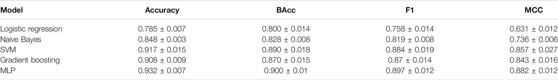
TABLE 3. Results for the classification of complexes on principal components. For each metric, the first column is the average over the results 10 runs of the cross-validation, while the second column is the standard deviation of these results.

In Figure 1, the distribution of objects in feature space for the extended dataset is presented. Although most of the objects fall within clear clusters of taxonomic groups, some of them are located much further from their main clusters, such as some objects of Q type and S type. This, on the one hand, poses a threat to the classification performance and, on the other hand, indicates that the spectra of those objects are much different than others in their group.

The promising results obtained in this experiment prove that it might be possible in the future to automatically assign taxonomic types of newly observed objects, where the spectral data are available. Furthermore, it serves as baseline for future research on different parameter combinations and their usability in predicting taxonomic types.

Classification With the Whole Spectra

Next, we verify whether the performance of the machine learning methods can be improved if the entire set of basic spectral features were used, rather than just the five first principal components. In this case, more information is being preserved, which could improve the accuracy, but it could also result in more variance due to a large number of possibly irrelevant features. Tables 4 and 5, respectively, show the results of this experiment for classification into the types and the complexes. It turns out that the prediction accuracy, measured by each evaluation metric, has consistently improved for the best performing methods (support vector machine, gradient boosting, and multilayer perceptron) for the case of predicting types. Two top-performing models, the multilayer perceptron (MLP) and support vector machine (SVM) obtained the balanced accuracy of 78% for types and 88% for complexes, where the MLP slightly outperforms the SVM on taxonomic types (78.8–78.2% BAcc, 0.781–0.761 F₁, and 0.805–0.787 MCC) and underperforms on complexes (88.4–88.9% BAcc, 0.886–0.889 F₁, and 0.873–0.876 MCC) for all metrics, while the difference is the most prominent on balanced metrics. Furthermore, the slight improvement in performance only occurs for MLP and SVM, while the other models perform worse than on the PCA set for both tasks. This is expected behavior for simpler models such as logistic regression and naive Bayes, which benefit highly from the reduced dimensionality of the input. The result of these experiments leads us to conclude that restricting to the top five principal components and the slope misses some part of the information about the classes available in the spectra when taxonomic types are being predicted. In the task of predicting complexes, the values of balanced accuracy for SVM are very similar between the PCA feature set and basic spectral feature set (around 89%) and slightly more different for MLP (90% for PCA to 88% for basic spectral features). In general, the results for complexes on PCA feature set are very similar, or even better than using the basic spectral features, which indicates that the top five principal components reflect the important information for differentiating complexes from the whole spectral range while reducing noise, which could negatively affect the classification.

TABLE 4

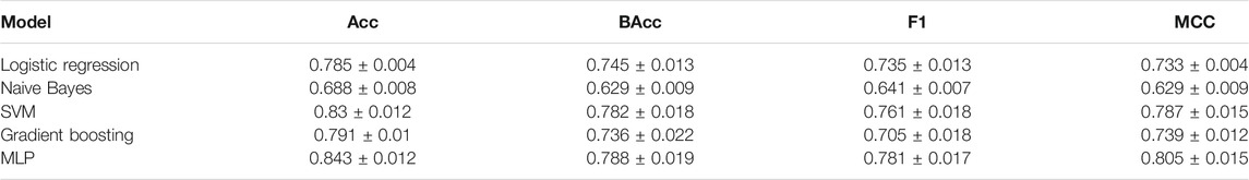
TABLE 4. Results for the classification of taxonomic types on basic spectral features. For each metric, the first column is the average over the results 10 runs of the cross-validation, while the second column is the standard deviation of these results.

TABLE 5

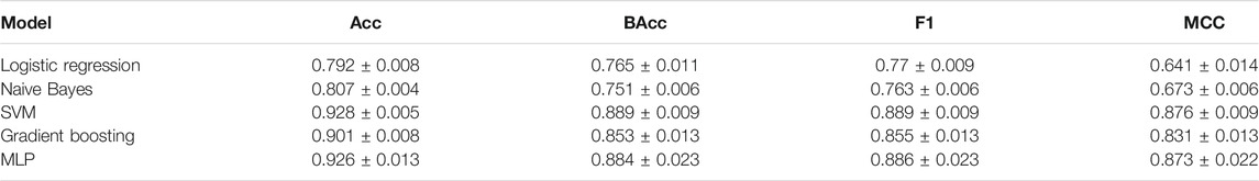
TABLE 5. Results for the classification of complexes on basic spectral features. For each metric, the first column is the average over the results 10 runs of the cross-validation, while the second column is the standard deviation of these results.

We complement the aforementioned results with the presentation of the confusion matrix for the classification of taxonomic types with the multilayer perceptron model using the basic spectral features (Figure 3). A confusion matrix in the k-class classification is a k-by-k matrix for which the entry in the ith row and the jth column (i, j = 1, … , k) gives the number of objects from class i classified to class j, thereby enabling to check which classes are most frequently confused by the model. Consistent with the results described before, the overall performance is very good, but the classifier produced errors across similar taxonomic types, that is, C and Ch, or S, Sq, and Sr, or X and Xk. It follows from this observation that the preprocessed spectra for those types are very similar and therefore hard to distinguish for the models. Spectral information might not be enough to separate those types. Further investigation into the spectra of types most commonly mistaken might be required as it might indicate the need of updating the taxonomic types of those objects.

FIGURE 3

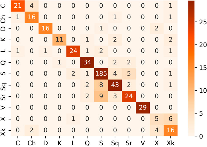
FIGURE 3. Confusion matrix for type prediction on basic spectral features with multilayer perceptron.

Feature Selection

Selection With Accuracy

Finally, the individual features are assessed through the sequential feature selection to quantify the importance of the features and track the improvement of performance with the increase in the feature set. The results of this experiment on complexes, presented in Tables 6 and 8, indicate that no more than five features are sufficient for the prediction accuracy of 94%. Slope was ranked as the most important feature for predicting complexes. In the second and third places, features 0.95 and 1.0 μm from a very close wavelength were ranked, and in fourth and fifth places, −1.15 and 1.25 μm. This not only indicates the importance of this region for classification but also shows that some of the similar features from this feature set are often exchanged with each other, and therefore excessive.

TABLE 6

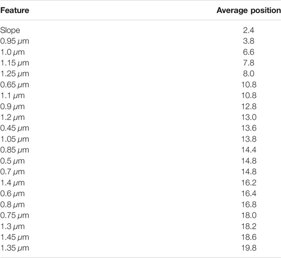
TABLE 6. Average rank per feature for the classification of complexes with accuracy during sequential feature selection on spectral features.

In the case of taxonomic type prediction, Tables 7 and 8 present that six features are enough for the prediction accuracy of 85%. The top features often selected in the early stages of feature selection were 0.9 μm, slope, and 0.95 μm. A group of similar points is ranked as the next best features: 1.35, 1.4, 1.1, and 1.05 μm.

TABLE 7

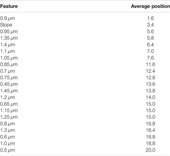
TABLE 7. Average rank per feature for the classification of taxonomic types with accuracy during sequential feature selection on spectral features.

TABLE 8

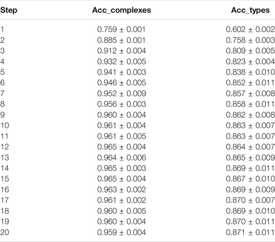
TABLE 8. Accuracy for the classification of complexes and types per step of sequential feature selection on spectral features.

Selection With Balanced Accuracy

A balanced metric was also used during the feature selection process, in order to assess the difference in selected features and reduce the negative impact of imbalanced class sizes. The balanced accuracy values of each step in sequential feature selection are presented in Table 9. For the prediction of complexes, the value of this metric was significantly lower in the first step (58% as opposed to 76% for accuracy) but leveled out in the next few steps, falling behind 1 percentage point upon reaching the fifth iteration, with the overall course of the experiment similar to the one with accuracy. Table 10 presents the ranking of features for the experiment on complexes. Among the top five features, the slope is again rated very high. Apart from that, similar wavelengths are selected, namely, 1.05, 0.9, and 1.1 μm, indicating the importance of this region for classification. Among the top five features, 0.65 μm was selected for the fourth place, while it was selected for sixth in the experiment with accuracy.

TABLE 9

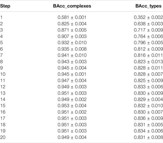
TABLE 9. Average rank per feature for the classification of complexes during sequential feature selection with balanced accuracy on spectral features.

TABLE 10

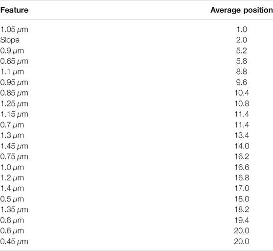
TABLE 10. Average rank per feature for the classification of taxonomic types during sequential feature selection with balanced accuracy on spectral features.

In the task of predicting taxonomic types, we can see the significant influence of selecting the balanced metric on the overall performance. The values of the balanced metric were lower than the accuracy, while the course of the experiment remained the same, achieving 80% in the fifth step. Among the six best features, there were some similarities as compared to the experiment with accuracy. Slope was again rated really high, as well as 0.9, 1.4 μm 0.95, and 1.05 μm were also selected early in the process, which is a very similar range of wavelengths as for the experiment with accuracy. As opposed to the experiment with accuracy, here the 0.65 μm wavelength was selected in the sixth place when it did not appear within the top 10 features for taxonomic type prediction when accuracy was used as a selection metric. The top features for predicting taxonomic types and complexes are presented in Figure 4.

FIGURE 4

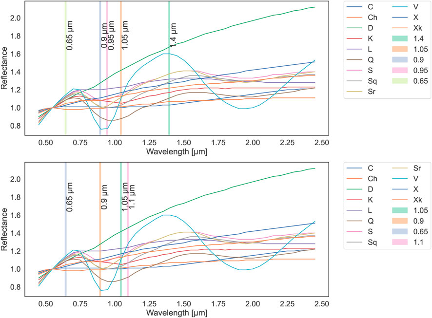
FIGURE 4. Most important spectral features in the task of taxonomic types (top) and complexes (bottom) prediction against mean reflectance values of taxonomic types used in classification, as measured with balanced accuracy.

It is worth noting that the feature selection process contains a random component, so when repeated, it is likely to lead to a slightly different set of features not only across different evaluation metrics but also within different runs with the same metric. Therefore, the differences in subsets between accuracy and balanced accuracy might naturally occur and might not be explainable other than due to the randomness of the process.

5 Discussion

The top features that we found (Tables 6, 7, 9, 11; Figure 4) correspond to the most prominent spectral characteristics. For classification of complexes, spectral slope and reflectance covering the 1-μm absorption band contributed to the majority of the classification with reflectances at other wavelengths providing much less information. This is not surprising, given that the slope is the most prominent feature of spectra and the 1-μm band is the main feature separating the complexes containing the 1-μm olivine/pyroxene absorption (S-complex and some types in the end-member population) from the featureless ones (C- and X-complexes). In the balanced accuracy experiment, the 0.65 μm hydration feature also ranked high. That hydrated minerals feature is present in many C-complex objects and the analog meteorites (Rivkin et al., 2002) and is uncommon in the more thermally transformed types (e.g., V-types from the end members group), which aids the separation of the end members. Furthermore, that parameter splits the C- and Ch-types and C from S/X complex objects, which are redder and typically have higher reflectance values at those wavelengths. Reflectances in the near-infrared part of the spectra did not appear among the top features for complex prediction. This is consistent with the fact that Bus–DeMeo retained the complex classification from the earlier Bus taxonomy, which was based on the visible part of the spectra only.

TABLE 11

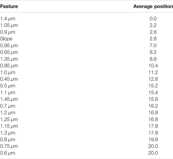
TABLE 11. Balanced accuracy for the classification of complexes and types per step of sequential feature selection on spectral features.

For the type classification based on spectra, the top features contributing to the classifications were slope and reflectances relating to 1-μm absorption band and interestingly spectra in the region 1.35–1.4 μm. That spectral region characterizes multiple types. For example, the Q- and Sq-types show a shallow feature around 1.3 μm; C- and Ch-types have a small positive slope that starts around 1.3 μm; D-types show a gentle kick around 1.35 μm; and the V-types show maximum reflectance in that range. That region does not have a clear mineralogical interpretation. Surprisingly, the 2-μm region ranked below the top 20 important features. In the DeMeo et al. (2009) taxonomy, the 2-μm pyroxene band was the most prominent feature clearly separating the space in the PCA component space. In the classification task, this feature seems redundant as other parameters cover spectral features of multiple other classes simultaneously and already provide a plenitude of information. The 2 μm feature may have also ranked higher if more types containing the feature (e.g., R, O, and Sv) were taken under the analysis, thus creating the need for characterizing the distinction in the reflectance values. Those types were skipped due to low number statistics.

Altogether the low number of features needed to classify objects is not surprising, and analogous to PCA in DeMeo et al. (2009), where the first 4–5 dimensions provide the most information and then the variance in the subsequent dimensions drops to essentially zero. Generally, the top features separating the types and complexes found by the machine learning algorithms appear to focus on reasonable traits of the spectra relating to physical characteristics of asteroids and analogous meteorites.

The 1-μm olivine/pyroxene absorption band appears in both the classification of types and complexes. It is one of two the most striking absorption bands in asteroid spectra tied to olivine and pyroxene content (Gaffey et al., 1993; Sanchez et al., 2014). For the classification of complexes, it is a clear distinction between olivine-containing asteroids (S-complex, V-types, and Q-types) and the rest. For the classification of types, it additionally helps assessing the depth of the absorption band.

It is worth noting that the S-complex asteroids were found broadly compatible with ordinary chondrites (OC) based on the 1-μm absorption band (Chapman and Salisbury, 1973) and after understanding that the space weathering processes affect the spectral slopes, causing the asteroid spectra to appear redder than that of meteorites (Sasaki et al., 2001; Chapman, 2004; Strazzulla et al., 2005). Furthermore, the Hayabusa sample return space missions provided mineralogical argument connecting the OC meteorites with S-complex asteroids (Nakamura et al., 2011; Yurimoto et al., 2011). However, as indicated by Vernazza et al. (2016) and others, the S-complex asteroids are a diverse group, and other meteorite groups may originate from this complex as well.

On the other hand, the hydrated Ch/Cgh-type asteroids (that do not contain the 1-μm band) are partly linked with CM chondrites (Rivkin, 2012; Bland and Travis, 2017; Vernazza et al., 2017; Carry et al., 2019). Hiroi et al. (1993) also suggested a link with the CI/CM meteorites. Some C-types that do not show hydration have also been linked to IDPs Vernazza et al. (2015); Carry et al. (2021). Part of the C-complex is not sampled by the meteorite collection Vernazza et al. (2015), which highlights some of the challenges in linking asteroid spectral types with their meteorite analogs.

The featureless types are mostly distinguished by their spectral slopes. For the X-complex, we only included the X and Xk types, which tend to have a higher spectral slope than that of the C-complex objects (C, Ch) considered in this study. The Xk types are considered parent bodies of mesosiderates (Vernazza et al., 2009b). The X-type in the Bus–DeMeo taxonomy does not distinguish the E, M, and P Tholen types (known as X-complex degeneracy) and thus may correspond to multiple meteorite groups.

During our analysis, we excluded several spectra types for which there were not enough data (Sa, Sv, B, Cb, Cg, Cgh, Xc, Xe, Xn, T, A, O, and R). These rare types are not classified in our analysis. Since we are performing fivefold stratified cross-validation, we require at least five spectra in each type. Moreover including objects with low number statistics may lead to a bias-variance tradeoff phenomenon, that is, overfitting. It is most evident for complex models like multilayer perceptrons.

The exclusion means that some classes and their features are not represented in our data set. Therefore, the top features that we found do not optimize those classes. Penttilä et al. (2021) merged those subclasses with their main equivalent (Sa with S). Although this process increases sample size, it may negatively influence the inference for the merged types. Furthermore, merging several subtypes into a single class may lead the machine learning algorithms toward the conclusion that the features that discriminate between them are irrelevant. Therefore, we decided to omit those types altogether.

The spectral data were not corrected for multiple factors such as phase reddening, temperature, grain size, space weathering effects, or impact darkening. Many of those mechanisms are poorly constrained for the different taxonomic types and sometimes even object-dependent.

The spectra of S-complex asteroids show redder spectral slopes with increasing phase angle (the effect is known as phase reddening), and the depth of the one- and two-micron bands increases up to 70 and 55 of phase angle, respectively, and then decreases (Sanchez et al., 2012). However, most main-belt asteroids are observed in the phase angle range 0–30°, where the effect is minuscule. The effect plays a more important role for near-Earth asteroids (NEAs) that can be observed at higher phase angles. Binzel et al. (2019) demonstrated the phase reddening effect for 433) Eros and explored the slope correction values for a few other asteroids. Based on that Binzel et al. (2019) suggested that the effect may be object-dependent and thus not easily accounted for.

Particle size affects the depth and slope of absorption features and overall reflectance. Large particle sizes typically result in deeper absorption bands, bluer spectral slope, and lower reflectance Reddy et al. (2015); Mustard and Hays (1997). Generally, larger asteroids tend to have smaller grain sizes as revealed by thermal inertia studies (Delbo et al., 2015). However, the grain size distribution for most individual asteroids (except those visited by space missions) is unknown thus correcting for particle size is impossible.

Temperature causes changes in the band centers and depths as well as broadens or narrows down the bands (thus also affects the bar area ratios) (Singer and Roush (1985); Hinrichs and Lucey (2002); Burbine et al. (2009)). The variation in temperature is more significant for objects on eccentric orbits like NEAs and less for main-belt objects.

Shock impact darkening can suppress the absorption bands and reduce the overall reflectance, which can lead to misclassification of objects (Kohout et al., 2020, 2014) as it tends to “move” objects even between complexes. Overall, phase reddening corrections play an important role in constraining the space reddening as they mostly affect spectral slope (Reddy et al., 2015). Temperature variations and shock impact darkening have a larger impact on mineralogical characterization (Reddy et al., 2015).

All the listed mechanisms affect our understanding of the asteroid–meteorite connection. However, applying corrections for the aforementioned factors is not viable with the current state of knowledge for all the asteroids of different taxonomic types in our sample.

Furthermore, the Bus–DeMeo taxonomy is simply based on observed spectral features and was not controlled for those factors. By training to recreate the Bus–DeMeo types, we trained to classify objects based on biased data into the Bus–DeMeo biased classes. Thus, those mechanisms do not affect our results.

However, these mechanisms can significantly affect asteroid spectra and have to be considered when new taxonomies, possibly based on much larger data, are derived (e.g., that based on the Gaia space mission data (Cellino et al., 2020)). Last, as shown by the OSIRIS-REx mission, rubble-pile asteroids may contain a mixture of various materials, like the basaltic exogenic material found on a primitive asteroid (101,955) Benu (DellaGiustina et al., 2021). Another example of such mixed exogenous composition is asteroid 2008 TC3 that impacted the Earth on October 7, 2008, and the recovered fragments contained many different ureilitic and chondritic lithologies (Bischoff et al., 2010). How common those objects are and how should they be handled in future taxonomies have to be carefully considered.

Our analysis did not take into account albedo information. In contrast to the Tholen taxonomy, the Bus–DeMeo taxonomy did not take into account geometric albedo, thus introducing that the additional parameter could confuse the classification of types in the X-complex (otherwise split into E, M, and P types in the Tholen taxonomy) or at the very least be a spurious parameter that does not contribute to the classification of classes that are not defined by albedo. Furthermore, as shown by the confusion matrix, there are more misclassifications within the complexes, which have similar albedos (except for the X-complex). Since we focus on the Bus–DeMeo taxonomy, we do not include geometric albedo in our analysis as well.

6 Conclusion

In this study, we addressed the automatic classification of taxonomic types and complexes according to the DeMeo et al. (2009) taxonomy. We assessed machine learning methods’ capability of recreating the classification with the data used in DeMeo et al. (2009) to create the taxonomy. We showed that machine learning methods can be used to recreate the Bus–DeMeo taxonomy. Moreover, this taxonomic scheme is robust in the sense that most of the types and complexes remain in place, despite the increased sample size, which is not always the case for taxonomies based on PCA analysis when more data are available.

Furthermore, the experiments were carried out to record the difference in performance on the spectra, rather than five principal components. We found that the prediction accuracy improved across both tasks and all methods, which proves that the original feature set misses some important information required to distinguish different types and complexes. In our experiments, a multilayer perceptron with three layers of 32 neurons, a stochastic gradient descent solver, batch size of 32, and adaptive learning rate with the initial value of 0.1 performed best for both tasks, closely followed by the support vector machine with the RBF kernel.

Sequential feature selection was performed on the task of taxonomic type prediction to quantify the importance of individual features. In the experiments, the feature set was reduced to highlight the areas of interest that mostly contribute to making the prediction. For complex prediction, the top five features were sufficient for obtaining 93% prediction balanced accuracy, whereas six features resulted in 81% balanced accuracy in the case of taxonomic type prediction. This shows that the whole spectrum contains redundant features which are not informative for predicting the output. On the one hand, this may lead to degradation of classification, due to overfitting to noise. On the other hand, it shows spectra contain more information than necessary for taxonomic-type prediction and that validates the reduction to a few narrowband filters.

For future space and ground-based surveys that aim for taxonomic characterization of asteroids in the Bus–DeMeo scheme, we would recommend the use of six narrowband filters that cover the reflectances at 0.65, 1.0, and 1.4 μm and additional couple filters that allow for estimation of the spectral slope in the 0.45–2.5 μm. According to this study, those would be sufficient to obtain prediction balanced accuracy on the level of 93 and 81% for prediction complexes and types, respectively. Narrowband filters were already utilized in the J-PLUS survey (Morate et al., 2021); however, those could be further optimized to more efficiently link the observed asteroids to the Bus–DeMeo taxonomy.

Data Availability Statement

Publicly available datasets were analyzed in this study. These data can be found here: http://smass.mit.edu/minuspubs.html.

Author Contributions

WK and DO conceived the presented idea. HK developed codes used for analysis and performed the computations. WK supervised HK and verified the results. FDM provided data and comments. HK wrote majority of the manuscript, with the exception of introductory and discussion sections written by DO. DO contributed to part of abstract and conclusions. All authors provided comments to the manuscript.

Funding

This work has been supported by grant No. 2017/25/B/ST9/00740 from the National Science Centre, Poland.

Conflict of Interest

The authors declare that the research was conducted in the absence of any commercial or financial relationships that could be construed as a potential conflict of interest.

Publisher’s Note

All claims expressed in this article are solely those of the authors and do not necessarily represent those of their affiliated organizations, or those of the publisher, the editors, and the reviewers. Any product that may be evaluated in this article, or claim that may be made by its manufacturer, is not guaranteed or endorsed by the publisher.

Acknowledgments

All of the data utilized in this publication were obtained and made available by the MITHNEOS MIT-Hawaii Near-Earth Object Spectroscopic Survey. The IRTF is operated by the University of Hawaii under contract 80HQTR19D0030 with the National Aeronautics and Space Administration. The MIT component of this study is supported by NASA grant 80NSSC18K0849.

References

Barucci, M. A., Perna, D., Fornasier, S., Doressoundiram, A., Lantz, C., Popescu, M., et al. (2017). “Neoshield-2 Project: Final Results on Compositional Characterization of Small Neos,” in AAS/Division for Planetary Sciences Meeting Abstracts#, 49, 110–208.

Google Scholar

Binzel, R. P., DeMeo, F. E., Turtelboom, E. V., Bus, S. J., Tokunaga, A., Burbine, T. H., et al. (2019). Compositional Distributions and Evolutionary Processes for the Near-Earth Object Population: Results from the Mit-hawaii Near-Earth Object Spectroscopic Survey (Mithneos). Icarus 324, 41–76. doi:10.1016/j.icarus.2018.12.035

CrossRef Full Text | Google Scholar

Bischoff, A., Horstmann, M., Pack, A., Laubenstein, M., and Haberer, S. (2010). Asteroid 2008 TC3-Almahata Sitta: A Spectacular Breccia Containing many Different Ureilitic and Chondritic Lithologies. Meteoritics Planet. Sci. 45, 1638–1656. doi:10.1111/j.1945-5100.2010.01108.x

CrossRef Full Text | Google Scholar

Bishop, C. M. (2006). Pattern Recognition and Machine Learning (Information Science and Statistics). Berlin, Heidelberg: Springer-Verlag. chap. 4.3.4.

Google Scholar

Bland, P. A., and Travis, B. J. (2017). Giant Convecting Mud Balls of the Early Solar System. Sci. Adv. 3, e1602514. doi:10.1126/sciadv.1602514

PubMed Abstract | CrossRef Full Text | Google Scholar

Bolin, B. T., Fremling, C., Holt, T. R., Hankins, M. J., Ahumada, T., Anand, S., et al. (2020). Characterization of Temporarily Captured Minimoon 2020 CD3by Keck Time-Resolved Spectrophotometry. ApJ 900, L45. doi:10.3847/2041-8213/abae69

CrossRef Full Text | Google Scholar

Burbine, T. H., Buchanan, P. C., Dolkar, T., and Binzel, R. P. (2009). Pyroxene Mineralogies of Near-Earth Vestoids. Meteoritics Planet. Sci. 44, 1331–1341. doi:10.1111/j.1945-5100.2009.tb01225.x

CrossRef Full Text | Google Scholar

Burbine, T. H., Meibom, A., and Binzel, R. P. (1996). Mantle Material in the Main belt: Battered to Bits. Meteoritics Planet. Sci. 31, 607–620. doi:10.1111/j.1945-5100.1996.tb02033.x

CrossRef Full Text | Google Scholar

Bus, S., and Binzel, R. P. (2002). Phase II of the Small Main-Belt Asteroid Spectroscopic Survey A Feature-Based Taxonomy. Icarus 158, 146–177. doi:10.1006/icar.2002.6856

CrossRef Full Text | Google Scholar

Bus, S. J. (1999). Compositional Structure in the Asteroid belt: Results of a Spectroscopic Survey. Ph. D. Thesis. Boston, MA: Massachusetts Institute of Technology, 311.

Google Scholar

Carry, B., Solano, E., Eggl, S., and DeMeo, F. E. (2016). Spectral Properties of Near-Earth and mars-crossing Asteroids Using sloan Photometry. Icarus 268, 340–354. doi:10.1016/j.icarus.2015.12.047

CrossRef Full Text | Google Scholar

Carry, B. (2018). Solar System Science with Esa euclid. A&A 609, A113. doi:10.1051/0004-6361/201730386

CrossRef Full Text | Google Scholar

Carry, B., Vachier, F., Berthier, J., Marsset, M., Vernazza, P., Grice, J., et al. (2019). Homogeneous Internal Structure of Cm-like Asteroid (41) daphne. A&A 623, A132. doi:10.1051/0004-6361/201833898

CrossRef Full Text | Google Scholar

Carry, B., Vernazza, P., Vachier, F., Neveu, M., Hanus, J. B. J., Ferrais, M., et al. (2021). Evidence for Differentiation of the Most Primitive Small Bodies. arXiv preprint arXiv:2103.06349.

Google Scholar

Carvano, J. M., Hasselmann, P. H., Lazzaro, D., and Mothé-Diniz, T. (2010). Sdss-based Taxonomic Classification and Orbital Distribution of Main belt Asteroids. A&A 510, A43. doi:10.1051/0004-6361/200913322

CrossRef Full Text | Google Scholar

Cellino, A., Bendjoya, P., Delbo’, M., Galluccio, L., Gayon-Markt, J., Tanga, P., et al. (2020). Ground-based Visible Spectroscopy of Asteroids to Support the Development of an Unsupervised Gaia Asteroid Taxonomy. A&A 642, A80. doi:10.1051/0004-6361/202038246

CrossRef Full Text | Google Scholar

Chapman, C. R., Morrison, D., and Zellner, B. (1975). Surface Properties of Asteroids: A Synthesis of Polarimetry, Radiometry, and Spectrophotometry. Icarus 25, 104–130. doi:10.1016/0019-1035(75)90191-8

CrossRef Full Text | Google Scholar

Chapman, C. R., and Salisbury, J. W. (1973). Comparisons of Meteorite and Asteroid Spectral Reflectivities. Icarus 19, 507–522. doi:10.1016/0019-1035(73)90078-x

CrossRef Full Text | Google Scholar

Chapman, C. R. (2004). Space Weathering of Asteroid Surfaces. Annu. Rev. Earth Planet. Sci. 32, 539–567. doi:10.1146/annurev.earth.32.101802.120453

CrossRef Full Text | Google Scholar

Chen, T., and Guestrin, C. (2016). “XGBoost,” in Proceedings of the 22nd ACM SIGKDD International Conference on Knowledge Discovery and Data Mining, New York, NY, USA (New York, NY: ACM, KDD), 16, 785–794. doi:10.1145/2939672.2939785

CrossRef Full Text | Google Scholar

de León, J., Licandro, J., Serra-Ricart, M., Pinilla-Alonso, N., and Campins, H. (2010). Observations, Compositional, and Physical Characterization of Near-Earth and mars-crosser Asteroids from a Spectroscopic Survey. A&A 517, A23. doi:10.1051/0004-6361/200913852

CrossRef Full Text | Google Scholar

Delbo, M., Mueller, M., Emery, J. P., Rozitis, B., and Capria, M. T. (2015). Asteroid Thermophysical Modeling. Tucson, AZ: University of Arizona Press Tucson, Arizona.

Google Scholar

DellaGiustina, D. N., Kaplan, H. H., Simon, A. A., Bottke, W. F., Avdellidou, C., Delbo, M., et al. (2021). Exogenic basalt on Asteroid (101955) Bennu. Nat. Astron. 5, 31–38. doi:10.1038/s41550-020-1195-z

CrossRef Full Text | Google Scholar

DeMeo, F. E., Binzel, R. P., Carry, B., Polishook, D., and Moskovitz, N. A. (2014). Unexpected D-type Interlopers in the Inner Main belt. Icarus 229, 392–399. doi:10.1016/j.icarus.2013.11.026

CrossRef Full Text | Google Scholar

DeMeo, F. E., Binzel, R. P., Slivan, S. M., and Bus, S. J. (2009). An Extension of the Bus Asteroid Taxonomy into the Near-Infrared. Icarus 202, 160–180. doi:10.1016/j.icarus.2009.02.005

CrossRef Full Text | Google Scholar

DeMeo, F. E., and Carry, B. (2014). Solar System Evolution from Compositional Mapping of the Asteroid belt. Nature 505, 629–634. doi:10.1038/nature12908

PubMed Abstract | CrossRef Full Text | Google Scholar

DeMeo, F. E., Polishook, D., Carry, B., Burt, B. J., Hsieh, H. H., Binzel, R. P., et al. (2019). Olivine-dominated A-type Asteroids in the Main belt: Distribution, Abundance and Relation to Families. Icarus 322, 13–30. doi:10.1016/j.icarus.2018.12.016

CrossRef Full Text | Google Scholar

Devogèle, M., Moskovitz, N., Thirouin, A., Gustaffson, A., Magnuson, M., Thomas, C., et al. (2019). Visible Spectroscopy from the mission Accessible Near-Earth Object Survey (Manos): Taxonomic Dependence on Asteroid Size. Aj 158, 196. doi:10.3847/1538-3881/ab43dd

CrossRef Full Text | Google Scholar

Erasmus, N., Mommert, M., Trilling, D. E., Sickafoose, A. A., Van Gend, C., and Hora, J. L. (2017). Characterization of Near-Earth Asteroids Using Kmtnet-Saao. Aj 154, 162. doi:10.3847/1538-3881/aa88be

CrossRef Full Text | Google Scholar

Gaffey, M. J., Bell, J. F., Brown, R. H., Burbine, T. H., Piatek, J. L., Reed, K. L., et al. (1993). Mineralogical Variations within the S-type Asteroid Class. Icarus 106, 573–602. doi:10.1006/icar.1993.1194

CrossRef Full Text | Google Scholar

Gil-Hutton, R., and Licandro, J. (2010). Taxonomy of Asteroids in the Cybele Region from the Analysis of the sloan Digital Sky Survey Colors. Icarus 206, 729–734. doi:10.1016/j.icarus.2009.10.010

CrossRef Full Text | Google Scholar

Goodfellow, I. J., Bengio, Y., and Courville, A. (2016). Deep Learning. Cambridge, MA, USA: MIT Press. http://www.deeplearningbook.org.

Google Scholar

Harris, A., and Davies, J. K. (1999). Physical Characteristics of Near-Earth Asteroids from thermal Infrared Spectrophotometry. Icarus 142, 464–475. doi:10.1006/icar.1999.6248

CrossRef Full Text | Google Scholar

Hastie, T., Tibshirani, R., and Friedman, J. (2009). The Elements of Statistical Learning: Data Mining, Inference and Prediction. 2 edn. Springer.

Google Scholar

Hinrichs, J. L., and Lucey, P. G. (2002). Temperature-dependent Near-Infrared Spectral Properties of Minerals, Meteorites, and Lunar Soil. Icarus 155, 169–180. doi:10.1006/icar.2001.6754

CrossRef Full Text | Google Scholar

Hiroi, T., Pieters, C. M., Zolensky, M. E., and Lipschutz, M. E. (1993). Evidence of thermal Metamorphism on the C, G, B, and F Asteroids. Science 261, 1016–1018. doi:10.1126/science.261.5124.1016

PubMed Abstract | CrossRef Full Text | Google Scholar

Jenniskens, P., Vaubaillon, J., Binzel, R. P., DeMEO, F. E., Nesvorný, D., Bottke, W. F., et al. (2010). Almahata Sitta (=asteroid 2008 TC3) and the Search for the Ureilite Parent Body. Meteoritics Planet. Sci. 45, 1590–1617. doi:10.1111/j.1945-5100.2010.01153.x

CrossRef Full Text | Google Scholar

Jolliffe, I. (2002). Principal Component Analysis. 2 edn. doi:10.1007/b98835

CrossRef Full Text | Google Scholar

Jones, R. L., Jurić, M., and Ivezić, Ž. (2015). Asteroid Discovery and Characterization with the Large Synoptic Survey Telescope. Proc. IAU 10, 282–292. doi:10.1017/s1743921315008510

CrossRef Full Text | Google Scholar

Kelleher, J. D., Namee, B. M., and D’Arcy, A. (2015). Fundamentals of Machine Learning for Predictive Data Analytics: Algorithms, Worked Examples, and Case Studies. MIT Press.

Google Scholar

Kingma, D., and Ba, J. (2014). “Adam: A Method for Stochastic Optimization,” in International Conference on Learning Representations.

Google Scholar

Kohout, T., Gritsevich, M., Grokhovsky, V. I., Yakovlev, G. A., Haloda, J., Halodova, P., et al. (2014). Mineralogy, Reflectance Spectra, and Physical Properties of the Chelyabinsk LL5 Chondrite - Insight into Shock-Induced Changes in Asteroid Regoliths. Icarus 228, 78–85. doi:10.1016/j.icarus.2013.09.027

CrossRef Full Text | Google Scholar

Kohout, T., Petrova, E. V., Yakovlev, G. A., Grokhovsky, V. I., Penttilä, A., Maturilli, A., et al. (2020). Experimental Constraints on the Ordinary Chondrite Shock Darkening Caused by Asteroid Collisions. A&A 639, A146. doi:10.1051/0004-6361/202037593

CrossRef Full Text | Google Scholar

Licandro, J., Popescu, M., Morate, D., and de León, J. (2017). V-type Candidates and vesta Family Asteroids in the Moving Objects vista (Movis) Catalogue. A&A 600, A126. doi:10.1051/0004-6361/201629465

CrossRef Full Text | Google Scholar

Marsset, M., DeMeo, F. E., Binzel, R. P., Bus, S. J., Burbine, T. H., Burt, B., et al. (2020). Twenty Years of Spex: Accuracy Limits of Spectral Slope Measurements in Asteroid Spectroscopy. ApJS 247, 73. doi:10.3847/1538-4365/ab7b5f

CrossRef Full Text | Google Scholar

McCord, T. B., Adams, J. B., and Johnson, T. V. (1970). Asteroid vesta: Spectral Reflectivity and Compositional Implications. Science 168, 1445–1447. doi:10.1126/science.168.3938.1445

PubMed Abstract | CrossRef Full Text | Google Scholar

Mignard, F., Cellino, A., Muinonen, K., Tanga, P., Delbò, M., Dell’Oro, A., et al. (2007). The Gaia mission: Expected Applications to Asteroid Science. Earth Moon Planet. 101, 97–125. doi:10.1007/s11038-007-9221-z

CrossRef Full Text | Google Scholar

Mommert, M., Trilling, D. E., Borth, D., Jedicke, R., Butler, N., Reyes-Ruiz, M., et al. (2016). First Results from the Rapid-Response Spectrophotometric Characterization of Near-Earth Objects Using Ukirt. Astronomical J. 151, 98. doi:10.3847/0004-6256/151/4/98

CrossRef Full Text | Google Scholar

Morate, D., Carvano, J. M., Alvarez-Candal, A., De Prá, M., Licandro, J., Galarza, A., et al. (2021). J-plus: A First Glimpse at Spectrophotometry of Asteroids–The Mooja Catalog. arXiv preprint arXiv:2106.00713.

Google Scholar

Mustard, J., and Hays, J. (1997). Effects of Hyperfine Particles on Reflectance Spectra from 0.3 to 25 μm☆. Icarus 125, 145–163. doi:10.1006/icar.1996.5583

CrossRef Full Text | Google Scholar

Nakamura, T., Noguchi, T., Tanaka, M., Zolensky, M. E., Kimura, M., Tsuchiyama, A., et al. (2011). Itokawa Dust Particles: a Direct Link between S-type Asteroids and Ordinary Chondrites. Science 333, 1113–1116. doi:10.1126/science.1207758

PubMed Abstract | CrossRef Full Text | Google Scholar

Navarro-Meza, S., Mommert, M., Trilling, D. E., Butler, N., Reyes-Ruiz, M., Pichardo, B., et al. (2019). First Results from the Rapid-Response Spectrophotometric Characterization of Near-Earth Objects Using Ratir. Aj 157, 190. doi:10.3847/1538-3881/ab1138

CrossRef Full Text | Google Scholar

Oszkiewicz, D. A., Kwiatkowski, T., Tomov, T., Birlan, M., Geier, S., Penttilä, A., et al. (2014). Selecting Asteroids for a Targeted Spectroscopic Survey. A&A 572, A29. doi:10.1051/0004-6361/201323250

CrossRef Full Text | Google Scholar

Pedregosa, F., Varoquaux, G., Gramfort, A., Michel, V., Thirion, B., Grisel, O., et al. (2011). Scikit-learn: Machine Learning in Python. J. Machine Learn. Res. 12, 2825–2830.

Google Scholar

Penttilä, A., Hietala, H., Muinonen, K., et al. (2021). Asteroid Spectral Taxonomy Using Neural Networks. Astron. Astrophysics 649, A46. doi:10.1051/0004-6361/202038545

CrossRef Full Text | Google Scholar

Popescu, M., Licandro, J., Carvano, J. M., Stoicescu, R., de León, J., Morate, D., et al. (2018). Taxonomic Classification of Asteroids Based on Movis Near-Infrared Colors. A&A 617, A12. doi:10.1051/0004-6361/201833023

CrossRef Full Text | Google Scholar

Popescu, M., Licandro, J., Morate, D., de León, J., Nedelcu, D. A., Rebolo, R., et al. (2016). Near-infrared Colors of Minor Planets Recovered from vista-vhs Survey (Movis). A&A 591, A115. doi:10.1051/0004-6361/201628163

CrossRef Full Text | Google Scholar

Reddy, V., Dunn, T. L., Thomas, C. A., Moskovitz, N. A., and Burbine, T. H. (2015). Mineralogy and Surface Composition of Asteroids. Asteroids IV, 183–204. doi:10.2458/azu_uapress_9780816532131-ch003

CrossRef Full Text | Google Scholar

Rivkin, A. S., Howell, E. S., Vilas, F., and Lebofsky, L. A. (2002). Hydrated Minerals on Asteroids:. Asteroids III 1, 235–254. doi:10.2307/j.ctv1v7zdn4.23

CrossRef Full Text | Google Scholar

Rivkin, A. S. (2012). The Fraction of Hydrated C-Complex Asteroids in the Asteroid belt from Sdss Data. Icarus 221, 744–752. doi:10.1016/j.icarus.2012.08.042

CrossRef Full Text | Google Scholar

Roig, F., and Gil-Hutton, R. (2006). Selecting Candidate V-type Asteroids from the Analysis of the sloan Digital Sky Survey Colors. Icarus 183, 411–419. doi:10.1016/j.icarus.2006.04.002

CrossRef Full Text | Google Scholar

Ruder, S. (2016). An Overview of Gradient Descent Optimization Algorithms. arXiv preprint arXiv:1609.04747.

Google Scholar

Sanchez, J. A., Reddy, V., Kelley, M. S., Cloutis, E. A., Bottke, W. F., Nesvorný, D., et al. (2014). Olivine-dominated Asteroids: Mineralogy and Origin. Icarus 228, 288–300. doi:10.1016/j.icarus.2013.10.006

CrossRef Full Text | Google Scholar

Sanchez, J. A., Reddy, V., Nathues, A., Cloutis, E. A., Mann, P., and Hiesinger, H. (2012). Phase Reddening on Near-Earth Asteroids: Implications for Mineralogical Analysis, Space Weathering and Taxonomic Classification. Icarus 220, 36–50. doi:10.1016/j.icarus.2012.04.008

CrossRef Full Text | Google Scholar

Sasaki, S., Nakamura, K., Hamabe, Y., Kurahashi, E., and Hiroi, T. (2001). Production of Iron Nanoparticles by Laser Irradiation in a Simulation of Lunar-like Space Weathering. Nature 410, 555–557. doi:10.1038/35069013

PubMed Abstract | CrossRef Full Text | Google Scholar

Scott, E., Goldstein, J., Yang, J., Asphaug, E., and Bottke, W. (2010). Iron and Stony-Iron Meteorites and the Missing Mantle Meteorites and Asteroids. Meteoritics Planet. Sci. Suppl. 73, 5015.

Google Scholar

Sergeyev, A., Carry, B., Onken, C., Devillepoix, H., Wolf, C., and Chang, S.-W. (2021). Multi-filter Photometry of Solar System Objects from the Skymapper Southern Survey. arXiv preprint arXiv:2110.11656. doi:10.1051/0004-6361/202142074

CrossRef Full Text | Google Scholar

Singer, R. B., and Roush, T. L. (1985). Effects of Temperature on Remotely Sensed mineral Absorption Features. J. Geophys. Res. 90, 12434–12444. doi:10.1029/jb090ib14p12434

CrossRef Full Text | Google Scholar

Solontoi, M. R., Hammergren, M., Gyuk, G., and Puckett, A. (2012). AVAST Survey 0.4-1.0μm Spectroscopy of Igneous Asteroids in the Inner and Middle Main belt. Icarus 220, 577–585. doi:10.1016/j.icarus.2012.05.035

CrossRef Full Text | Google Scholar

Strazzulla, G., Dotto, E., Binzel, R., Brunetto, R., Barucci, M. A., Blanco, A., et al. (2005). Spectral Alteration of the Meteorite Epinal (H5) Induced by Heavy Ion Irradiation: A Simulation of Space Weathering Effects on Near-Earth Asteroids. Icarus 174, 31–35. doi:10.1016/j.icarus.2004.09.013

CrossRef Full Text | Google Scholar

Sykes, M., Cutri, R. M., Fowler, J. W., Tholen, D. J., Skrutskie, M. F., Price, S., et al. (2000). The 2mass Asteroid and Comet Survey. Icarus 146, 161–175. doi:10.1006/icar.2000.6366

CrossRef Full Text | Google Scholar

Tholen, D. J. (1989). Asteroid Taxonomic Classifications. Asteroids II, 1139–1150.

Google Scholar

Vernazza, P., Binzel, R. P., Rossi, A., Fulchignoni, M., and Birlan, M. (2009a). Solar Wind as the Origin of Rapid Reddening of Asteroid Surfaces. Nature 458, 993–995. doi:10.1038/nature07956

PubMed Abstract | CrossRef Full Text | Google Scholar

Vernazza, P., Brunetto, R., Binzel, R. P., Perron, C., Fulvio, D., Strazzulla, G., et al. (2009b). Plausible Parent Bodies for Enstatite Chondrites and Mesosiderites: Implications for Lutetia's Fly-By. Icarus 202, 477–486. doi:10.1016/j.icarus.2009.03.016

CrossRef Full Text | Google Scholar

Vernazza, P., Castillo-Rogez, J., Beck, P., Emery, J., Brunetto, R., Delbo, M., et al. (2017). Different Origins or Different Evolutions? Decoding the Spectral Diversity Among C-type Asteroids. Aj 153, 72. doi:10.3847/1538-3881/153/2/72

CrossRef Full Text | Google Scholar

Vernazza, P., Marsset, M., Beck, P., Binzel, R. P., Birlan, M., Brunetto, R., et al. (2015). Interplanetary Dust Particles as Samples of Icy Asteroids. ApJ 806, 204. doi:10.1088/0004-637x/806/2/204

CrossRef Full Text | Google Scholar

Vernazza, P., Zanda, B., Nakamura, T., Scott, E., and Russell, S. (2016). The Formation and Evolution of Ordinary Chondrite Parent Bodies. arXiv preprint arXiv:1611.08734.

Google Scholar

Virtanen, P., Gommers, R., Oliphant, T. E., Haberland, M., Reddy, T., Cournapeau, D., et al. (2020). SciPy 1.0: Fundamental Algorithms for Scientific Computing in Python. Nat. Methods 17, 261–272. doi:10.1038/s41592-019-0686-2

PubMed Abstract | CrossRef Full Text | Google Scholar

Wetherill, G., Chapman, C., Kerridge, J., and Matthews, M. (1988). Meteorites and the Early Solar System. Tucson: University of Arizona Press, 35–67.

Google Scholar

Whitney, A. W. (1971). A Direct Method of Nonparametric Measurement Selection. IEEE Trans. Comput. C-20, 1100–1103. doi:10.1109/T-C.1971.223410

CrossRef Full Text | Google Scholar

Yurimoto, H., Abe, K.-i., Abe, M., Ebihara, M., Fujimura, A., Hashiguchi, M., et al. (2011). Oxygen Isotopic Compositions of Asteroidal Materials Returned from Itokawa by the Hayabusa mission. Science 333, 1116–1119. doi:10.1126/science.1207776

PubMed Abstract | CrossRef Full Text | Google Scholar

Zellner, B., Tholen, D. J., and Tedesco, E. F. (1985). The Eight-Color Asteroid Survey: Results for 589 minor Planets. Icarus 61, 355–416. doi:10.1016/0019-1035(85)90133-2

CrossRef Full Text | Google Scholar