Charge-Exchange Byproduct Cold Protons in the Earth’s Magnetosphere

1 Introduction

In the dipolar portions of the Earth’s magnetosphere, ring current ions charge exchange with the neutral hydrogen exosphere of the Earth, which is known as the hydrogen geocorona (Carruthers et al., 1976; Rairden et al., 1986). For an energetic proton H⁺_energetic (expression (1a)), an energetic nitrogen ion N⁺_energetic (expression (1b)), or an energetic oxygen ion O⁺_energetic (expression (1c)), the charge-exchange reaction can be expressed as

${\text{H}}_{\text{energetic}}^{+}{+\text{ H}}_{\text{low}-\text{energy}}^{\text{0}}\to {\text{ H}}_{\text{energetic}}^{\text{0}}{+\text{ H}}_{\text{low}-\text{energy}}^{+},(\mathrm{1a})$

${\text{N}}_{\text{energetic}}^{+}{+\text{ H}}_{\text{low}-\text{energy}}^{\text{0}}\to {\text{ N}}_{\text{energetic}}^{\text{0}}{+\text{ H}}_{\text{low}-\text{energy}}^{+},(\mathrm{1b})$

${\text{O}}_{\text{energetic}}^{+}{+\text{ H}}_{\text{low}-\text{energy}}^{\text{0}}\to {\text{ O}}_{\text{energetic}}^{\text{0}}{+\text{ H}}_{\text{low}-\text{energy}}^{+},(\mathrm{1c})$

${\text{He}}_{\text{energetic}}^{+}{+\text{ H}}_{\text{low}-\text{energy}}^{\text{0}}\to {\text{ He}}_{\text{energetic}}^{\text{0}}{+\text{ H}}_{\text{low}-\text{energy}}^{+},(\mathrm{1d})$

where an energetic (∼10’s of keV) ion passes near a low-energy (less than an eV) hydrogen atom, and the result of the reaction is an energetic hydrogen atom or an energetic nitrogen atom or an energetic oxygen atom and, in all three cases, a low-energy proton. Charge exchange with the geocorona is an important process for the decay of the ring current (Smith and Bewtra, 1978; Kistler et al., 1989; Liemohn et al., 1999; Ilie et al., 2013; Ilie and Liemohn, 2016) and for the creation of unstable hot-ion distribution functions in the dipolar magnetosphere (Cornwall, 1977; Thomsen et al., 2011, Thomsen et al., 2017). In recent years, the space-physics community has become interested in this charge-exchange process because remote detection of the energetic atoms can allow the imaging of the ring current/geocorona overlap (e.g., Gruntman, 1997; Perez et al., 2016). In this report, the cold byproduct protons from the charge-exchange reactions are of great interest.

Charge-exchange byproduct protons are discussed briefly in Delzanno et al. (2021). At the 1998 GEM Summer Workshop, Pat Reiff posed a question after a presentation as to whether charge exchange could be an important source for the refilling of the plasmasphere (Borovsky et al., 1998a). This work is an outgrowth from that question.

This article is organized as follows: In Section 2, the expected properties of charge-exchange byproduct protons in the magnetosphere are described. In Section 3, two methods are used to estimate the rate of production of cold charge-exchange protons in the dipolar magnetosphere. In Section 4, computer simulations are performed to look at the global population of cold charge-exchange byproduct protons in the magnetosphere under varying levels of geomagnetic activity. In Section 5, the role of cold charge-exchange byproduct protons in the transition from early stage to late stage plasmaspheric refilling is assessed In Section 6, the results are summarized, and a new work is called for that will refine the conclusions of this report.

2 Properties of Charge-Exchange Byproduct Protons

As ion-plasma-sheet (ring current) ions are convected into the dipolar magnetosphere from the near-Earth portions of the magnetotail, they encounter the neutral hydrogen geocorona of the Earth. The density of the geocorona falls off with the distance from the Earth. In Figure 1 (cf. Fig. 1 of Ilie et al., 2013), the neutral-hydrogen number density is plotted at the equator at local midnight as a function of the distance from the Earth: here, power-law fits to five geocorona models are plotted in the five different colors. The models from Rairden et al. (1986) are in black, Hodges (1994) in blue, Ostgaard et al. (2003) in red, Bailey and Gruntman (2011) in green, and Zoennchen et al. (2011) in light blue. The power-law fits to the number density (in units of cm⁻³) are displayed in the figure. As can be seen, the density of neutral hydrogen increases strongly approaching the Earth, and so the probability of charge exchange increases greatly as an ion approaches the Earth.

FIGURE 1

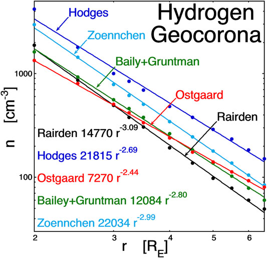
FIGURE 1. Number density of the hydrogen geocorona as a function of the distance from the Earth’s center along the Sun–Earth line in the nightside (local midnight). The plotted curves are from five different models of the geocorona. Power-law fits to the curves are displayed in the figure (after Ilie et al., 2013)).

Because of this strong radial dependence, the cold byproduct protons of charge-exchange origin are predominantly born at high latitudes. The ion plasma sheet is relatively isotropic (at geosynchronous orbit, T_perp/T_|| values are typically in the 1 to 1.3 range for the <40-eV portion of the ion plasma sheet (Denton et al., 2005)), so there are significant numbers of ions that mirror at high latitudes in the dipolar magnetosphere. As the ions bounce in the magnetic flux tubes, they approach the Earth at high latitudes and spend more time there, where the geocoronal density is higher and so where the probability for charge exchange is higher. Assuming that the hot-ion distribution is isotropic at the equator, Liouville’s theorem indicates that the hot-ion distribution will be isotropic everywhere away from the equator and that its number density will be everywhere the same as it is at the equator (cf. Borovsky and Cayton, 2011; Sect. 4.4 of Roederer and Zhang, 2014). For an isotropic hot-ion population at geosynchronous orbit (L = 6.6), this constant density is exploited to obtain the effective flux-tube–averaged number density of the geocorona, which is found to be 2.09 times the equatorial number density if n_geoc ∝ r^−3.09 (e.g., the black curve in Figure 1), and the flux-tube–averaged number density of the geocorona is 1.64 times the equatorial number density if n_geoc ∝ r^−2.44 (e.g., the red curve in Figure 1) (See Jordanova et al. (1996) or Liemohn and Kozyra (2003) for bounce averaging when the hot-ion distribution is not isotropic). At 6.5 R_E, the average value of the geocoronal number density n_geoc of the five curves in Figure 1 is 82 cm⁻³. So, if the boost in density given by flux-tube–averaging is 1.85 times (the average of the five power laws in Figure 1) the equatorial value, then the geosynchronous midnight flux tube has an effective geocorona density n_geoc of about 152 cm⁻³.

Figure 2 examines the production of charge-exchange byproduct protons in a flux tube as a function of latitude assuming the hot-ion distribution is isotropic at the equator. In that case, the number density of hot ions is independent of latitude, and the relative rate of production of charge-exchange byproduct protons depends only on the cross section of the flux tube as a function of latitude. For a dipole geosynchronous flux tube, the figure plots the rate of production of byproduct protons in the flux tube relative to the rate of production at the equator. The blue curve accounts only for the decreasing volume of the flux tube with increasing latitude: this would be the relative production curve, if the number density of the neutral hydrogen geocorona was uniform and did not vary with the distance from the Earth. The red curve in Figure 2 is the relative rate of production as a function of latitude accounting for both the reduced volume of the dipolar flux tube with increasing latitude and the increasing number density of the geocorona with closeness to the Earth (A n_geoc ∝ r^−2.8 case was taken for the red curve, with 2.8 being the mean value of the five exponents in Figure 1.). As can be seen comparing the red curve to the blue curve, the n_geoc ∝ r^−2.8 geocorona greatly increases the byproduct-proton production at high latitudes. The median value of the blue distribution is at 14.0°, and the median value of the red distribution is at 25.5°. For the red curve, half of the byproduct cold protons produced in the flux tube are produced at a latitude higher than 25.5°, and half of the byproduct protons are produced at a latitude lower than 25.5°.

FIGURE 2

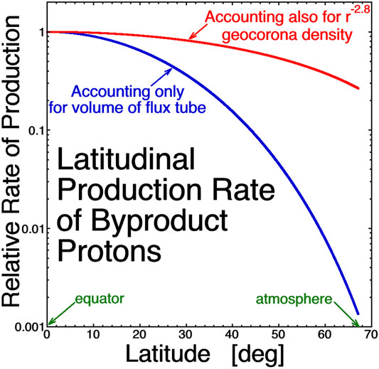
FIGURE 2. In a dipole flux tube at geosynchronous orbit, the latitudinal distribution of the rate of production of charge-exchange byproduct protons is plotted for an isotropic distribution of energetic ions in the flux tube. The blue curve would be the case if the geocoronal density did not vary with the distance from the Earth, and the red curve is the case for a geocoronal density that varies as r^−2.8.

Since the byproduct protons from charge exchange are born predominantly away from the equator, the population of cold byproduct protons will be somewhat field-aligned at the equator owing to the enhanced birth rate of byproduct protons at portions of the flux tube away from the equator (essentially, the cold ions produced at each latitude in the flux tube will produce a sort of “inverse loss cone” population at the equator). If the hot-ion population in a flux tube is isotropic at the equator, it will be isotropic everywhere in the flux tube. If the hot-ion population is isotropic, then the cold byproduct protons will be produced with isotropic velocity vectors. The excess byproduct protons produced off the equator will show up at the equator as an excess of field-aligned protons.

The byproduct protons are born with low kinetic energies and are probably born with isotropic velocity distributions. The kinetic energies of the gravitationally bound geocoronal hydrogen atoms can be estimated with the use of the virial theorem, which states that for a circular orbit, the orbital kinetic energy ε_kin is one-half of the gravitational potential energy ε_pot. Thus,

${\mathrm{\epsilon }}_{\text{kin}}=\text{ G M m / }2\text{r,}(2)$

where G = 6.67 × 10⁻⁸ cm⁻³ gm⁻¹ s⁻² is the gravitational constant, M = 5.97 × 10²⁷ gm is the mass of the Earth, m = 1.67 × 10⁻²⁴ gm is the mass of a hydrogen atom, and r is the distance from the center of the Earth. At geocentric-orbit distances (r = 6.6 R_E = 4.2 × 10⁹ cm), the kinetic energy of a geocoronal hydrogen atom is ε_kin∼7.9 × 10⁻¹⁴ erg = 0.05 eV.

By kinematically analyzing the laboratory measurements of the deflection angles of fast protons that have undergone charge exchange with hydrogen atoms, it can be determined that the cold byproduct protons from charge exchange are born with very little kinetic energy. In a charge-exchange collision with a cold atom (assuming a spherically symmetric scatter potential), the fast proton with velocity v_energetic and kinetic energy ε_energetic = mv_energetic²/2 will be deflected by an angle θ_defl and will transfer a kinetic energy ε_collision to the cold atom, with the cold atom becoming a cold proton. Using conservation of energy and momentum and assuming that the particle masses are identical, one finds that the kinetic energy received by the cold atom converted into a proton is

${\mathrm{\epsilon }}_{\text{collision}}={\mathrm{\epsilon }}_{\text{energetic }}{\text{sin}}^2\left({\mathrm{\theta }}_{\text{defl}}\right)\text{/}\left({1+\text{sin}}^2\left({\mathrm{\theta }}_{\text{defl}}\right)\right).(3)$

For a wide range of incident-proton energies, Table 1 shows measured values of the maximum deflection angle of the fast proton as a function of its incident energy. The majority of charge-exchange events will occur at deflection angles below these quoted maximum deflection angles, which were qualitatively obtained from the published differential cross sections (Chen et al., 1973; Toshima et al., 1989; Gaussorgues et al., 1975; Schinke and Kruger, 1976; Martin et al., 1981). Using these values, the maximum energy imparted to the byproduct protons is calculated from expression (2), and these values are collected into Table 1. As can be seen from the table, the energies of the charge-exchange byproduct protons will be less than 0.6 eV for incident proton energies in the range from 500–125 keV, which covers the ion plasma sheet. This small energy transfer makes sense since charge exchange is a tunneling process that can occur at larger distances than scattering between a proton and a neutral hydrogen atom. Consistent with this, it will be seen in Section 3 that the charge-exchange cross section for a 1-keV hydrogen atom is ∼20 times the cross-sectional area of the hydrogen atom. Note that the momentum transferred to the byproduct proton in the charge-exchange collision is in a direction that is nearly orthogonal to the initial trajectory of the fast ion. Since the velocity kick received by the byproduct proton during the charge-exchange collision is nearly transverse to the path of the fast proton, for an isotropic distribution of fast protons the byproduct protons are born with an isotropic velocity distribution.

TABLE 1

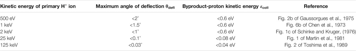
TABLE 1. Estimates of byproduct-proton kinetic energies from kinematic analysis of measured primary deflection angles.

If a byproduct proton is born in the corotational electric field, the cold byproduct proton will pick up a gyrational energy ε_pickup that is comparable to the corotational kinetic energy where it is born. If a proton is born at a distance ρ from the rotational axis of the Earth, this energy gain is

${\mathrm{\epsilon }}_{\text{pickup}}=1{\text{.}1\text{×}10}^{-3}\text{ eV}{\left(\mathrm{\rho /}{1\text{ R}}_{\text{E}}\right)}^2.(4)$

Even if ρ = 10 R_E, this energy is considerably less than 1 eV. Outside the corotational region, E×B convection can be faster. But even if the convection speed is 10 km/s (5.7 R_E/h), the pickup kinetic energy ε_pickup will only be 0.52 eV.

It is possible that the byproduct protons can pick up parallel kinetic energies owing to parallel electrostatic potential differences that may exist in the dipolar magnetosphere. Substantial potential drops between the ionosphere and the magnetosphere are common in the auroral zone, as indicated by the inverted-V in low-altitude electron spectrograms (which map to the electron plasma sheet (Feldstein and Galperin, 1993)) and as also seen in downward-current regions (Lynch et al., 2002). The auroral zone can extend to L-shells lower than geosynchronous orbit on the nightside (Mauk and Meng, 1991; Motoba et al., 2015; Ozaki et al., 2015), particularly when the geomagnetic activity is high. Another source of field-aligned potential drops is the ambipolar electric field driven by the emission of photoelectrons from the upper atmosphere (Khazanov et al., 1997; Glocer et al., 2017). The photoelectron-driven potential drops are a few volts, so byproduct protons born at high latitudes could pick up a few eV of parallel kinetic energy. Ambipolar field-aligned potentials can also be set up, if the hot ions and hot electrons of the magnetosphere have different degrees of anisotropy (Persson, 1963; Lennartsson, 1976; Chiu and Schulz, 1978; Stern, 1981). This property is exploited to produce electrostatic ion confinement in laboratory mirror machines (e.g., Hershkowitz et al., 1982). One can imagine that the magnetospheric hot ions have an effective anisotropy that changes with time as the hot-ion population decays owing to charge exchange. These anisotropy-driven ambipolar potentials can be a fraction of the hot-particle temperatures (Whipple, 1977), so a parallel potential of at least a few volts driven by multi-keV ions and electrons is almost probable. Should the byproduct protons gain parallel kinetic energy owing to any of these parallel potential differences in the magnetosphere, they will appear as a cold, field-aligned proton beam in the equatorial magnetosphere.

A candidate population of cold ions that may be the byproduct protons produced by hot-ion charge exchange with the geocorona is seen in the equatorial magnetosphere at geosynchronous orbit by the Magnetospheric Plasma Analyzer (MPA) (Bame et al., 1993). An example of this ion population can be seen in the energy-time ion spectrogram as shown in Figure 3. Here, 3.8 h of ion measurements are shown from the spacecraft LANL-02A on September 23, 2003. The spacecraft was crossing the nightside in geosynchronous orbit at the equator. The vertical axis of the spectrogram is the logarithm of the ion energy going from 1 eV at the bottom to 40 keV at the top. The color is the intensity of the ion energy flux at that energy. On the horizontal axis, UT is plotted with the local time of the spacecraft indicated in parentheses: in the plot, the spacecraft travels from about 22.7 LT to about 2.5 LT. The vertical black lines in Figure 3 denote the time interval when the spacecraft was in eclipse. The feature in the spectrogram to focus on is the narrow “ion line” that has darkness below it. In the hot electron plasma sheet, the MPA spacecraft charges to large negative potentials with respect to the ambient magnetospheric plasma (Thomsen et al., 2013): any low-energy ions in the magnetospheric plasma are accelerated across this potential to produce this narrow-energy (cold) line in the energy-time spectrogram. The energy of the ion line is used as a direct measure of the spacecraft potential with respect to infinity (Borovsky et al., 1998b). The vertical width of the ion line is narrow, indicating that the energy spread of the ions is small compared with the potential that the ions fell through. At around 21 UT in Figure 3, the potential of the ion line is about 30 V, and the line is still narrow. There are 40 evenly spaced energy channels in the spectrogram, so at 21 UT the energy spread in the ion-line population is much less than 30 eV. The density in the ambient magnetospheric plasma of these cold ions is difficult to determine owing to the sheath focusing by the large-radius and large-voltage spacecraft sheath (for example, at 19 UT in Figure 3, the hot-electron density is 0.51 cm⁻³ and the hot-electron temperature is 4.2 keV yielding a Debye length for the spacecraft of λ_De = 0.68 km). Preliminary calculations based on orbit-limited ion collection indicate that the densities of the cold ambient protons that produce the ion lines at high voltages are on the order of 10⁻² cm⁻³. It is believed that the ion-line ions with their low-ambient fluxes are only detectable because the spacecraft charges to high-negative potentials so that its sheath collecting area is much greater than its surface area (e.g., Chen, 1965; Hershkowitz, 1989).

FIGURE 3

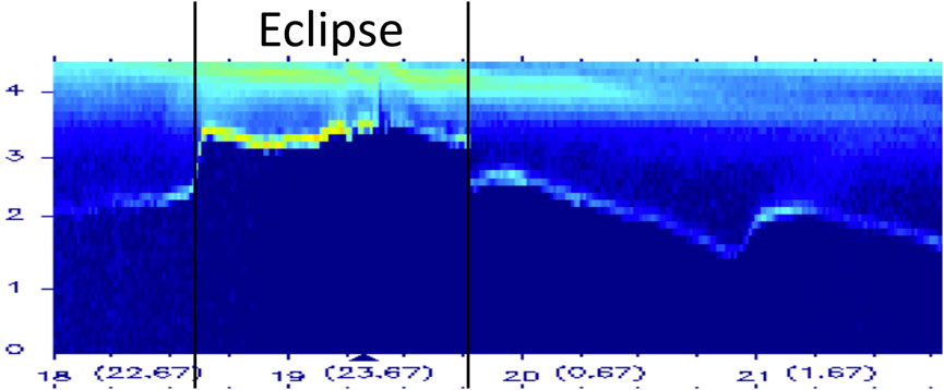
FIGURE 3. 3.8-h long energy-time ion spectrogram taken from the MPA instrument on September 23, 2003, onboard the spacecraft LANL-02A at geosynchronous orbit crossing the nightside. The energy resolution of the spectrogram is 40 vertical channels logarithmically spaced. The time resolution is 86 s.

3 Production Estimates for Byproduct Protons

In this section, the rate of production of cold protons owing to the charge exchange of ion-plasma-sheet (ring current) ions with geocoronal hydrogen atoms is estimated in two different ways. In the first method, the total number of plasma-sheet protons passing into the dipolar region per day is considered, and then the fraction lost owing to charge exchange is applied to these to obtain the total number of charge-exchange collisions in the dipolar region of the magnetosphere per day. The second method involves examining the number density and temperature of the ion plasma sheet at geosynchronous orbit, estimating the density of the geocorona there, and applying measured charge-exchange cross sections to these numbers to obtain the rate of charge-exchange collisions at geosynchronous orbit. Then, similar calculations will be carried out to determine the rate of production of cold protons by electron-impact ionization of the geocorona hydrogen atoms by electron-plasma-sheet electrons and the rate of production of cold protons by photoionization of the geocorona hydrogen atoms. The values are collected in Table 2.

TABLE 2

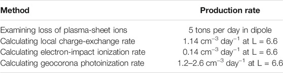
TABLE 2. Estimates of the number of byproduct cold protons produced.

The first calculation proceeds as follows: The proton mass of the earthward-convecting portion of the ion plasma sheet M_ps on the nightside of the Earth is about 1,150 kg (Table 4 of Borovsky et al.(1998c)), assuming that all of the plasma-sheet ions are protons. This material convects from the near-Earth magnetotail, into the dipolar region of the magnetosphere, past the Earth’s terminators, to the dayside magnetopause where it is lost. The convection time τ_conv (replacement time) for the nightside plasma sheet is estimated to be about 2.1 h (Table 4 of Borovsky et al.(1998c)). This gives a mass flow rate of M_ps/τ_conv ∼ 1.3 × 10⁴ kg/day of hot protons into the dipole from the magnetotail, which is about 13 metric tons per day. By comparing the number density of the ion plasma sheet on the dayside of the dipolar region at geosynchronous orbit with its number density on the nightside of the dipolar region, a rough estimate of the fraction of ion-plasma-sheet ions that undergo charge exchange can be obtained. At geosynchronous orbit, the ion-plasma-sheet number density on the nightside is typically n_night ∼ 0.7 cm⁻³, and the density on the dayside is n_day ∼ 0.4 cm⁻³ (e.g., Korth et al., 1999). This represents a ∼40% loss in the ions in passing the dipole from the nightside to the dayside (the loss is probably slightly higher since the flux-tube volume is larger on the nightside of geosynchronous orbit than it is on the dayside; the equatorial field strength being typically ∼30% less on the nightside than it is on the dayside (Rufenach et al., 1992; Borovsky and Denton, 2010)). Assuming that the density reduction is solely due to charge-exchange loss (ignoring loss of hot protons to the atmosphere), the ∼40% of 1.3 × 10⁴ kg/day represents a ∼5 × 10³ kg/day loss of hot protons owing to charge exchange. For every hot proton lost to charge exchange, one cold byproduct proton is produced. Hence, ∼5 × 10³ kg/day, or ∼5 metric tons per day, of cold protons are produced in the dipolar magnetosphere as byproducts of charge exchange. This value is entered into Table 2. This number should be taken as an order-of-magnitude estimate, since the mass of the plasma sheet is difficult to discern, and the estimated convection time for the plasma sheet differs depending on whether ionospheric or magnetospheric flows are analyzed. The number density of the plasma sheet also varies considerably from day-to-day depending on solar-wind conditions (Borovsky et al., 1998d). As a comparison to the five tons per day of byproduct protons, the mass of the protons in the outer filled plasmasphere (the region that tends to drain and refill) is on the order of 34 tons (Borovsky and Steinberg, 2006).

The second calculation, which estimates the rate of occurrence R of charge-exchange collisions at geosynchronous orbit, proceeds as follows: the rate of production of byproduct protons (number per unit time per unit volume) is

${\text{R }=\text{ n}}_{\text{energetic}}\text{ f,}(5)$

where n_energetic is the number density of hot (energetic) ions, and f is the frequency that one of these energetic ions undergoes charge-changing collisions. For the number density and temperature of the hot protons at geosynchronous orbit at local midnight, the values n_energetic = 0.88 cm⁻³ and T_energetic = 8.9 keV are taken from the upper-right geosynchronous-orbit point in Fig. 2 of Borovsky et al., (1998c). The frequency f of charge-exchange collisions for a proton in the hydrogen geocorona is

${\text{f }=\text{ n}}_{\text{geoc}}{\text{ v}}_{\text{energetic}}\mathrm{\sigma ,}(6)$

where n_geoc is the number density of hydrogen atoms in the geocorona, v_energetic is the velocity of the energetic proton, and σ is the charge-exchange cross section for a proton on a hydrogen atom. For v_energetic, the velocity of a proton with a kinetic energy of 8.9 keV is taken, which is v_energetic = 1.3 × 10⁸ cm/s. For n_geoc, the mean value of the five curves in Figure 1 at r = 6.5 R_E is 82 cm⁻³, and an effective flux-tube average value (for an isotropic hot-ion distribution at the equator) is about 1.85 times that of the equatorial density, yielding n_geoc = 152 cm⁻³ for the “bounce-averaged” geocorona number density (cf. Section 2). The measured charge-exchange cross section σ for a proton is plotted in the top panel of Figure 4 as a function of the proton kinetic energy, taken from the data in Table A-22 of Barnett (1990), which is a compilation of a number of laboratory experiments. Note, in the top panel, the large size of this cross section at 1 keV is σ = 1.7 × 10⁻¹⁵ cm², which is 19.4 times than that of the cross-sectional area of a hydrogen atom πa_o² = 8.8 × 10⁻¹⁷ cm², where a_o = 5.29 × 10⁻⁹ cm is the Bohr radius and the radius of a hydrogen atom (cf. Table 1 of Ghosh and Biswas (2002)). A 1-keV proton coming within 4.4 atomic radii of a hydrogen atom can undergo charge exchange, hence the very weak kinetic energy transfer ε_collision to the byproduct proton during the exchange (cf. Section 2 and Table 1). At 8.9 keV, the charge-exchange cross section is σ = 8.3 × 10⁻¹⁶ cm². In the bottom panel of Figure 4, v_energeticσ is plotted. Ideally, to utilize expression (5) for a distribution of hot ions, one should average v_energeticσ over the distribution of ions (this is complicated because the distribution functions of plasma sheet ions at geosynchronous orbit are non-Maxwellian; e.g., see Fig. 9 of Birn et al.(1997)). Fortunately, in the energy range of the ions of the ion plasma sheet, the quantity v_energeticσ does not vary very much; as can be seen in the bottom panel of Figure 4, in the kinetic energy range from 100 eV to 50 keV, v_energeticσ varies by less than a factor of 4. For a distribution of protons with a temperature of about 8.9 keV, a value of v_energeticσ ≈ 1 × 10⁻⁷ cm⁻³ s⁻¹ will be used. Using these values in expression (6) with n_geoc ≈ 152 cm⁻³ yields a frequency of charge exchange of f ≈ 1.3 × 10⁻⁵ s⁻¹ (this represents a half-life to charge exchange of about 15 h for a hot proton at geosynchronous orbit). Using this value of f in expression (5) along with n_energetic ≈ 0.88 cm⁻³ yields a production rate of cold byproduct protons of R ≈ 1.3 × 10⁻⁵ cm⁻³ s⁻¹, which is 1.14 cm⁻³day⁻¹. This value is entered into Table 2.

FIGURE 4

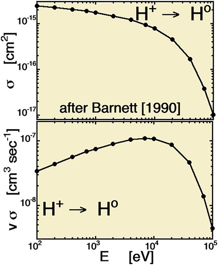
FIGURE 4. In the top panel, the charge-exchange cross section σ of a hydrogen atom to a proton is plotted as a function of the proton kinetic energy E (after Barnett (1990)). In the bottom panel, the product vσ is plotted as a function of E, where v is the proton velocity.

For comparison with the rate of production of cold protons by charge exchange, the rate of production of cold protons by electron-impact ionization of geocoronal hydrogen by the electron plasma sheet is estimated. Similar to the aforementioned calculation of charge-exchange production, the electron-impact ionization rate R will be

${\text{R }=\text{ n}}_{\text{elec}}{\text{ n}}_{\text{geoc}}{\text{ v}}_{\text{elec}}{\mathrm{\sigma }}_{\text{ioniz}},(7)$

where n_elec is the number density of hot electrons, v_elec is the velocity of a hot electron, σ_ioniz is the impact-ionization cross section for the hot electron on a hydrogen atom, and n_geoc is the density of hydrogen atoms. The number density of the hot electrons is taken to be n_elec = 0.88 cm⁻³, and the electron-plasma-sheet temperature is taken to be T_elec = 2 keV (cf. Fig. 2 of Denton et al.(2005)). The velocity of an electron with an energy of 2 keV is v_elec = 1.9 × 10⁹ cm/s. The electron-impact ionization cross section for a hydrogen atom to 2 keV electrons is σ_ioniz ≈ 6.3 × 10⁻¹⁸ cm⁻³ (e.g., Fig. 7 of Shah et al.(1987) or Fig. 5 of Tawara and Kato (1987)). Again, the bounce-averaged density of the hydrogen geocorona as seen by an isotropic population of electrons at L = 6.6 is n_geoc = 152 cm⁻³. Using these values in expression (7) yields a rate of ionization of R ∼ 1.6 × 10⁻⁶ cm⁻³ s⁻¹, which is R ∼ 0.14 cm⁻³ day⁻¹ at geosynchronous orbit. This value is entered into Table 2. For electron energies E_elec in the range from 400 eV to 4 keV, the quantity v_elecσ_ioniz varies with electron energy approximately as v_elecσ_ioniz ∝ E_elec^−0.35; hence, averaging over a thermal distribution of electrons does not greatly vary the value of v_elecσ_ioniz and R, and the value of R ∼ 0.14 cm⁻³ day⁻¹ is relatively insensitive to the temperature of the electrons of the electron plasma sheet (however, the rate R is sensitive to the number density of the hot electrons, which varies with time). This is the rate of production of cold protons by electron-impact ionization by the electron plasma sheet. This R ∼ 0.14 cm⁻³ day⁻¹ rate is about 12% of the 1.14 cm⁻³ day⁻¹ rate of production by charge exchange of the ion plasma sheet.

For another comparison, the rate of production of cold protons from solar photoionization of the neutral hydrogen geocorona is estimated. At 1 AU from the sun, the photoinization rate of a hydrogen atom is about 1 × 10⁻⁷ s⁻⁷ to 2 × 10⁻⁷ s⁻¹ (Gruntman, 1990; Ogawa et al., 1995), i.e., the lifetime of a hydrogen atom to photoionization is about 57–115 days. If the effective number density of the geocorona for a midnight geosynchronous-orbit flux tube is n_geoc = 152 cm⁻³, then the production rate from photoionization is on the order of 1.5 × 10⁻⁵ cm⁻³/s to 3 × 10⁻⁵ cm⁻³/s or 1.3–2.6 cm⁻³day⁻¹, which is comparable to the production rate from charge exchange. This value is entered into Table 2.

4 Magnetospheric Simulations of Byproduct-Proton Production and Transport

To explore the rudimentary behavior of the population of cold byproduct protons, numerical simulations are utilized. The HEIDI (Hot Electron Ion Drift Integrator) simulation code (Liemohn and Jazowski, 2008; Ilie et al., 2012) is used to look at the production and transport of the cold charge-exchange protons for two cases of steady geomagnetic activity. The HEIDI code simulates the evolution of the hot ring-current (ion-plasma-sheet) ion population by calculating the velocity moments of the ion phase–space distribution function through the dipolar magnetosphere, whose evolution is under the action of the E×B drift and gradient and curvature drifts. HEIDI includes hot-ion loss via charge exchange with the geocorona and loss to precipitation into the atmosphere. The outer boundary of the simulation is at L = 6.5 (approximately geosynchronous orbit), and a boundary condition for the simulations is that the number density and temperature of the hot ion plasma sheet (ring current) is specified at L = 6.5 on the nightside. In the two simulations, the Volland–Stern electric-field model (Volland, 1973; Stern, 1975) was used, parameterized by Kp. For the magnetic field, a non-tilted dipole was used. The HEIDI code incorporates a variety of neutral hydrogen geocorona models (Ilie et al., 2013); the Rairden et al.(1986) model for the neutral hydrogen geocorona is used for the two simulations.

The cold charge-exchange byproduct protons are advected via E×B in the simulations. The small losses of the cold protons 1) via scattering into the loss cone and 2) via charge exchange with the hydrogen geocorona are ignored in the simulations. The loss timescale for a 1-eV proton scattering into the atmosphere is estimated to be 89 h at L = 3 and 87 days at L = 6.6. The loss timescale for a 1-eV proton to charge exchange with the Hodges (1994) geocorona (the highest-density model in Figure 1) is 55 h at L = 3 and 370 h at L = 6.6. But, note that if a cold proton is lost to charge exchange, it is replaced by another cold proton.

For the two simulations, Figure 5 plots the number density of cold charge-exchange protons at near-geosynchronous orbit (L = 6.5) as a function of local time. Figure 5A is for a low-activity simulation in which Kp = 1, and the nightside number density of the ion plasma sheet was 0.93 cm⁻³ and the temperature was 5 keV; Figure 5B is for a very high-activity simulation in which Kp = 6, and the nightside number density of the ion plasma sheet was 1.45 cm⁻³ and the temperature was 11.6 keV. In both simulations, the ionic composition of the plasma sheet on the nightside was taken to be 100% H⁺, and so only cold protons produced by energetic protons charge exchanging with atomic hydrogen (expression (1a)) are calculated in the simulations. Each simulation was run for 72 h with a time-independent level of magnetospheric convection (parameterized by the steady level of Kp) and with a time-independent number density and temperature of the ion plasma sheet at L = 6.5 on the nightside. In the plots of Figure 5, the number density of cold charge-exchange protons is artificially low on the nightside at L = 6.5: the number density at L = 6.5 on the nightside is only related to the combination of production in the first outer cell of the code and advection out of that cell. In reality, there is production of cold protons beyond L = 6.5 on the nightside followed by advection through the L = 6.5 region; that production beyond L = 6.5 does not appear in the simulation since the outer boundary of the simulation domain is at L = 6.5. At local midnight in the simulations at 72 h, a comparison of the number density of cold byproduct protons at L = 6.5 and at L = 6.25 finds the density in the Kp = 1 simulation goes from 1.1 × 10⁻² at 6.6 to 4.6 × 10⁻² cm⁻³ at 6.25, and in the Kp = 6 simulation the density goes from 2.8 × 10⁻³ to 6.8 × 10⁻³ cm⁻³. This is a factor of ∼3 increase from L = 6.6 to L = 6.0, so if the production of byproduct cold protons beyond L = 6.5 was accounted for in the simulations, the number-density values at L = 6.5 on the nightside could easily triple. Note in Figure 5 that the cold-ion number density at local midnight is much less for the Kp = 6 case than it is for the Kp = 1 case: this is dominantly a function of the plasma advection strength where cold ions are more rapidly convected away in the Kp = 6 case but can build up in number density in the Kp = 1 case.

FIGURE 5

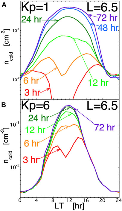
FIGURE 5. From two HEIDI simulations, the number density of cold charge-exchange byproduct protons is plotted in the equatorial plane at L = 6.5 as functions of local time. Panel (A) is for a Kp = 1 run with the nightside ion plasma sheet having n = 0.93 cm⁻³ and T = 5 keV, and panel (B) is for a Kp = 6 run with the nightside ion plasma sheet having n = 1.45 cm⁻³ and T = 11.6 keV.

The major production of charge-exchange cold protons is in the inner dipolar region where the neutral hydrogen geocorona is denser. The cold protons produced in the inner dipolar regions advect sunward, and so the number density of cold charge-exchange byproduct protons is relatively larger where they cross geosynchronous orbit on the dayside. In Figure 5, both simulations yield number densities of cold byproduct protons of 0.2–0.3 cm⁻³ at local noon at L = 6.5 (unfortunately, the ion-line analysis performed for the MPA spacecraft on the nightside, where there is strong charging, does not work on the dayside, where there is an absence of strong charging). Note, however, that the local-time width of the higher-density cold protons is narrow in the high-activity simulation (Figure 5B) and wide in the low-activity simulation (Figure 5A).

The number densities of charge-exchange byproduct protons are proportional to the number density of the ion plasma sheet flowing into the dipolar region on the nightside. It will also depend on the ion composition of the plasma sheet. Further, the (Rairden et al., 1986) geocorona model was used in the simulations of Figure 5: if another geocorona model were to be used (cf. Figure 1), the number density of cold byproduct protons would be higher.

At L = 6.5, the number density of cold charge-exchange byproduct protons is less than the number density of the ion plasma sheet. The peak cold-proton number densities of 0.2–0.3 are about half of the typical dayside ion-plasma-sheet densities n_day ∼ 0.4 cm⁻³ (e.g., Korth et al., 1999). For cold-ion measurements in the dayside magnetosphere, these byproduct cold-proton densities may be lost in the population of plasmaspheric-refilling outflows, which can result in number density buildups of 50 cm⁻³/day at geosynchronous orbit (Sojka and Wrenn, 1985; Lawrence et al., 1999; Su et al., 2001; Denton and Borovsky, 2014). In the following section, an assessment is made of the role that the cold charge-exchange byproduct proton distribution plays in the early time refilling of the plasmasphere in the dayside magnetosphere: it is found that the number densities of the byproduct protons are probably not sufficient to eliminate the early phase of refilling, but the byproduct population probably contributes to the shortening of the early phase, helping to bring on the transition to the rapid late phase refilling.

A study is in progress on the behavior of the cold charge-exchange byproduct proton population at all L-shells in simulations of the magnetospheric under time-dependent geomagnetic activity.

5 Cold Byproduct Protons and Early Time Plasmaspheric Refilling

On the dayside, the sunlit ionosphere has cold-proton outflows that can build up to refill the outer plasmasphere in the dipolar magnetosphere. It is argued that there are two different timescales for the refilling (Wilson et al., 1992; Lawrence et al., 1999; Su et al., 2001; Gallagher et al., 2021): a slow refilling at early times and a faster refilling at late times. (But see Denton and Borovsky (2014) for evidence against a two-timescale picture.)

Early refilling is slow because the protons coming out of one ionosphere ballistically traverse the length of the magnetospheric flux tube and end up lost in the conjugate atmosphere. It is argued that until there is sufficient cold plasma in the flux tube to sufficiently Coulomb scatter a transiting proton, that proton is likely to be lost in the conjugate atmosphere. Sufficient Coulomb scatter means enough angular scattering to knock the transiting proton out of the loss cone during its transit. To get to this stage where a transition to faster late-time refilling occurs, the amount of angular scattering per transit should be greater than or equal to the atmospheric loss cone as seen at the equator.

Equation (6.4.11) of Krall and Trivelpiece (1973) expresses the timescale τ for a thermal proton in a hydrogen plasma of density n and temperature T to be scattered through a total angle of 1 radian by multiple Coulomb scattering events. The timescale to scatter through the small loss-cone angle θ_loss is θ_loss² times this timescale, where θ_loss is expressed in radians. This gives

$\mathrm{\tau }={\mathrm{\theta }}_{\text{loss}}^2\left\{\left({\text{m}}_{\text{p}}^{1\text{/}2}{\left({\text{k}}_{\text{B}}\text{T}\right)}^{3\text{/}2}\right)\text{/}\left(2^{1\text{/}2}\mathrm{\pi }{\text{n e}}^4{\text{ log}}_{\text{e}}\left(\text{Λ}\right)\right)\right\}{[\text{0}\text{.}843+\text{ 0}\text{.}415]}^{-1}(\mathrm{A1})$

where log_e(Λ) is the Coulomb logarithm, 0.843 is a factor for the scattering of the proton by the electrons of the plasma, and 0.415 is a factor for the scattering of the proton by the protons of the plasma (Note that the square-bracket final factor []⁻¹ in expression (A1) is written incorrectly as []⁺¹ in eq. (6.4.11) of Krall and Trivelpiece (1973)). We are interested in the number density n that will produce a scattering by θ_loss in a time τ = d/v_o, where d is the transit pathlength through the plasma and v_o is the speed of the transiting proton. Using τ = d/v_o in expression (A1) and solving for n yields, we get

$\text{n}={\mathrm{\theta }}_{\text{loss}}^2\left\{\left({\text{m}}_{\text{p}}^{1\text{/}2}{\left({\text{k}}_{\text{B}}\text{T}\right)}^{3\text{/}2}{\text{v}}_{\text{o}}\right)/\left(2^{1\text{/}2}\mathrm{\pi }{\text{d e}}^4{\text{ log}}_{\text{e}}\left(\text{Λ}\right)\right)\right\}{[\text{0}\text{.}843+0\text{.}415]}^{-1}(\mathrm{A2})$

At the geosynchronous-orbit equator for a 100-nT field, the loss cone angle is θ_loss = 2.5° = 4.5 × 10⁻² radian. As the proton transits from one ionosphere to the other, any angular scattering that occurs at high latitude is not effective at moving the proton out of the loss cone; hence, for d, we will take a transit length at lower latitude in the dipolar flux tube. For L = 6.6, this length is taken to be d = 6.6 R_E = 4.2 × 10⁴ km. Taking the transiting proton to have an energy of 1 eV and the building-up proton–electron plasma in the magnetosphere to have that same 1-eV temperature, this gives T = 1 eV and v_o = 14 km/s. The Coulomb logarithm for a plasma with a temperature of 1 eV and a density of about 1 cm⁻³ is log_e(Λ) = 23. Using these values in expression (A2) yields the critical number density of a 1-eV proton–electron plasma to be n = 0.26 cm⁻³.

The number densities of charge-exchange byproduct protons can be non-negligible compared with this number density n = 0.26 cm⁻³ (cf. Figure 5). That 0.26 cm⁻³ number density was calculated for a T_i = T_e = 1-eV plasma. However, the cold charge-exchange byproduct protons are produced by removing hot protons (or hot O⁺ ions or hot N⁺ ions) from the magnetosphere and not altering the hot electrons, and so there is no 1-eV population of electrons accompanying the cold byproduct protons to help with the Coulomb scattering of a transiting proton (the hot ions and hot electrons in the flux tube are not effective at Coulomb scattering of a cold proton). Hence the factor [0.843 + 0.415]⁻¹ in expression (A2) becomes [0 + 0.415]⁻¹ for cold charge-exchange protons without accompanying cold electrons. This increases the calculated critical number density 0.26 cm⁻³ by a factor of 3.0, yielding a critical number density of byproduct protons of n = 0.79 cm⁻³ to cause a transition from slow early time refilling to fast late-time refilling. However, a number density of 0.2–0.3 cm⁻³ (cf. Figure 5) will do some angular scattering to shorten the time that early time refilling needs to go on before the transition density can be reached.

Also in the magnetospheric flux tube, there are the two “refilling” beams of protons from the ionospheric outflow that have non-zero number densities, and each beam contributes to the Coulomb scattering of the other beam. For these two beams to be able to account for the late-stage refilling rate of the plasmasphere R_late, each beam must have a number density n_beam at the equator of

${\text{n}}_{\text{beam}}=\left(2\text{/}2\right){\text{R}}_{\text{late}}{\mathrm{т}}_{\text{transit}},(\mathrm{A3})$

where τ_transit is the transit time from the ionosphere to the equator, the factor of 2 in the denominator accounts for the fact that two beams give rise to the refilling rate R_late so that each beam takes half the density, and the factor of 2 in the numerator accounts for the fact that the refilling is only on for about 12 h out of 24 h because the refilling only occurs from the sunlit ionosphere so the dayside refilling rate is twice the daily rate. The transit time in the dipole flux tube at geosynchronous orbit from the ionosphere to the equator is τ_transit = (1.3) (6.6) (1 R_E)/v_beam = 5.4 × 10⁴ km/v_beam. The measured late-stage refilling rate at geosynchronous orbit is 25–50 cm⁻³/day (Sojka and Wrenn, 1985; Lawrence et al., 1999; Su et al., 2001; Denton and Borovsky, 2014). For a 1-eV outflow beam of protons (with v_beam = 14 km/s), the transit time is τ_transit = 1.1 h, and the equatorial number density of each beam given by expression (A3) is n_beam = 1.1–2.2 cm⁻³. This is a substantially higher number density than the 0.2–0.3 cm⁻³ number densities of the cold charge-exchange byproduct proton population found at geosynchronous orbit in the HEIDI simulations (although the HEIDI simulations yielded densities that are lower bounds, owing to the use of the (Rairden et al., 1986) geocorona and the absence of charge exchange beyond L = 6.5 on the nightside). However, the effectiveness of proton–proton Coulomb scattering is very sensitive to the relative velocities of the colliding protons, and the protons of one beam pass the protons of the other beam with a relative speed v_o of 28 km/s whereas the protons of each beam pass through the byproduct protons with a relative speed v_o of about 14 km/s. To obtain the same angular-scattering effect, one needs a critical density n_crit that increases as n_crit ∝ ${\text{v}}_o^4$ (cf. expression (6.2.4) or (6.2.6) of Krall and Trivelpiece (1973)), so the density of a beam is not as effective as at scattering by a factor of about 4 as is the density of the byproduct protons are. Based on observations, the temperature of the outer plasmasphere may be higher when the plasmaspheric density is low, and the temperature is lower when the density is high (e.g., Comfort et al., 1985; Moldwin et al., 1995). There is some argument that the outflow energy of protons from the ionosphere is greater during early stage refilling than it is during late-stage refilling (cf. Wilson et al., 1992; Su et al., 1998). If the proton outflow energy is 3 eV (with v_beam = 24 km/s), then expression (A3) yields the equatorial number density of each beam to be n_beam = 0.65–1.3 cm⁻³, and if the proton outflow energy is 10 eV (with v_beam = 44 km/s), then expression (A3) yields the equatorial number density of each beam to be n_beam = 0.36–0.71 cm⁻³.

Note that in the dayside magnetosphere, there is also the oxygen-rich warm plasma cloak (Chappell et al., 2008). The ions of the cloak have been explored (Horwitz and Chappell, 1979; Borovsky et al., 2013; Lee and Angelopoulos, 2014; Takahashi et al., 2014; Jahn et al., 2017; Delzanno et al., 2021), but the electrons of the cloak are mostly a mystery (Li et al., 2011; Nishimura et al., 2013; Mozer et al., 2017; Walsh et al., 2020). The dayside cloak can have ion densities of a fraction of 1 cm⁻³ (cf. Fig. 9 of Jahn et al., 2017) or even higher than 1 cm⁻³ during storm times (cf. Fig. 20 of Borovsky et al., 2013). For a calculation, we take n = 0.2 cm⁻³ for the O⁺ of the cloak at geosynchronous orbit on the dayside (cf. Fig. 9 of Jahn et al., 2017). The temperature of the cloak varies (as does its number density), but for the sake of calculation we take the O⁺ temperature to be 20 eV. For Coulomb scattering, it is the relative velocity of the colliding particles that controls the strength of the scatter; 20-eV O⁺ ions have a velocity distribution very similar to that of 1-eV H⁺ ions. Note, however, that heavy O⁺ ions are more effective at angular scattering a transiting proton since an O⁺ ion recoils less than an H⁺ ion does during a collision, and so the transiting proton deflects more off of O⁺ than it does off of H⁺. Hence, 0.2 cm⁻³ of 20-eV cloak oxygen is probably a more important factor in ending the early time refilling phase than is 0.2–0.3 cm⁻³ of byproduct protons.

The densities of all of the populations (byproduct and cloak) vary with time, so at times the byproduct protons may play an important role in bringing about the transition from slow early time plasmasphere refilling to rapid late-time plasmasphere refilling.

6 Summary

In this report, the production of cold protons from charge-exchange collisions between the protons of the ion plasma sheet (ring current) and the neutral hydrogen geocorona was investigated, and the properties of these byproduct protons were ascertained.

The properties of the byproduct protons are as follows (see also Section 2): Each charge-exchange collision produces one byproduct proton. The byproduct protons are born primarily off equatorial in the dipolar portions of the magnetosphere, owing to the intersection of the quasi-isotropic ions of the ion plasma sheet and the radially decreasing density of hydrogen atoms in the Earth’s geocorona. When they are born, the byproduct protons are trapped in the magnetosphere by mirror geometry of the dipole magnetic field of the Earth. Since they are born primarily away from the equator, the distribution of cold protons will tend to be field aligned. The protons are born with very little kinetic energy (<0.6 eV) from the charge-exchange collisions, and they pick up very little energy (<1 eV) owing to the corotational and convectional electric field in which they are suddenly born. If there are field-aligned electrostatic potentials residing in the dipolar magnetosphere (driven perhaps by photoelectrons off the atmosphere, by anisotropies in the ion- and electron-plasma-sheet populations, by contact of the hot magnetospheric electrons with the ionosphere, or by field-aligned currents), then the byproduct protons may pick up a parallel-to-B kinetic energy.

A population of ions that are seen at the equator in geosynchronous orbit was identified as a candidate for being these byproduct protons produced by charge-exchange collisions (see Section 2). The population of ions is known as the “ion line” in energy-time ion spectrograms. The ion line is formed by ambient ions (with thermal energies less than a few 10’s of eV) that are accelerated across the spacecraft sheath from the ambient magnetospheric plasma to the negatively charged satellite. The ion line is typically seen in the midnight-to-dawn region of local time at geosynchronous orbit where satellites encounter the electron plasma sheet. At the equator, the cold ions of the ion line tend to be field aligned. The ambient densities of the cold ions that make up the line are estimated to be about ∼10⁻² cm⁻³ in the nightside magnetosphere at geosynchronous orbit. Without strong spacecraft charging (which occurs in the electron plasma sheet) and the associated strong sheath focusing of ion orbits onto the satellite, these ions would be difficult to detect with standard ion instruments.

The rates of production of byproduct protons from charge exchange were estimated by two different ways (see Section 3). By combining an estimate of the total flow of ion-plasma-sheet protons into the nightside of the dipolar region and an estimate of the fraction of those ion-plasma-sheet ions that are lost to charge exchange as they pass the dipole from the nightside to the dayside, the total number of charge-exchange collisions in the dipolar region was estimated: the estimate yields about 5 tons per day of cold byproduct protons in the magnetosphere. By examining the temperature and density of the ion plasma sheet at geosynchronous orbit (L = 6.6) and using a model of the neutral hydrogen geocorona, the rate of charge-exchange collisions was estimated: about 1.14 cm⁻³ per day of byproduct protons is produced in geosynchronous-orbit flux tubes on a typical day.

The rate of production of cold protons owing to electron-impact ionization of geocoronal hydrogen atoms by the electrons of the electron plasma sheet was estimated (see Section 3). About 0.14 cm⁻³ per day of cold protons is produced this way at geosynchronous orbit, predominantly on the nightside and dawnside. The production rate of cold protons by electron-impact ionization is a factor of 10 less than the production rate by charge exchange.

The rate of production of cold protons owing to solar photoionization of geocoronal hydrogen atoms was estimated (see Section 3). About 1.3–2.6 cm⁻³ per day of cold protons is produced this way at geosynchronous orbit. The production rate of cold protons by photoionization is comparable to or greater than the production rate by charge exchange.

The production and transport of cold byproduct protons was investigated with the HEIDI simulation code. Two steady-state convection runs were investigated (Kp = 1 and Kp = 6), and the number density at L = 6.5 in the equatorial plane was examined. Both simulations yielded byproduct-proton number densities that peaked on the dayside, with maximum number densities of 0.2–0.3 cm⁻³ near local noon (note that these number densities would be higher, perhaps by a factor of 2, if a geocorona model other than the Rairden et al., 1986 model would have been used in the simulations; further, the number densities are lowered by the fact that the charge-exchange production of protons beyond L = 6.5 on the nightside is not included). These number densities are small compared with expected number densities of plasmaspheric-refilling proton outflows from the ionosphere and are also small compared with dayside cloak-ion number densities. An assessment at geosynchronous orbit of the population of cold charge-exchange byproduct protons in the dayside magnetosphere finds that they likely contribute to the shortening of any “early phase” of plasmaspheric refilling by Coulomb scattering ionospheric-outflow protons out of the atmospheric loss cone, yielding a trapping of the outflows and a buildup of the magnetospheric plasmaspheric density.

To test whether or not the ions making the ion line are the predicted byproduct protons from charge exchange, the statistics of the observed properties of the “ion-line” population versus ion-plasma-sheet densities, magnetospheric convection rates, etc., are called for. If the ion-line ions are cold byproduct protons from charge-exchange collisions on the nightside of the dipolar region, then there should be a positive correlation between the density of the ion-line ions and the density of the ion plasma sheet, particularly when the convection age of the flux tube is accounted for. If there are factors that cause the density of the neutral hydrogen geocorona to vary (e.g., Banks and Kockarts, 1973; Bzowski and Fahr, 1996; Kuwabara et al., 2017), then the density of the ion line should also be affected by these factors, which can be tested observationally.

Data Availability Statement

The original contributions presented in the study are included in the article/Supplementary Material; further inquiries can be directed to the corresponding author.

Author Contributions

JB initiated this project, performed some of the analysis, and wrote the first draft of the manuscript. JL performed and analyzed the simulations under the supervision of RI. ML helped to write an earlier version of the manuscript. JL, RI, and ML helped to write the final version of the manuscript.

Funding

This work was supported at the Space Science Institute by the NSF GEM Program via grant AGS-2027569, by the NASA Heliophysics LWS program via award NNX16AB75G, by the NSF SHINE program via grant AGS-1723416, and by the NASA Heliophysics Guest Investigator Program via award NNX17AB71G. The work at the University of Michigan was supported by the NASA grants 80NSSC17K0015, NNX17AB87G, and 80NSSC19K0077.

Conflict of Interest

The authors declare that the research was conducted in the absence of any commercial or financial relationships that could be construed as a potential conflict of interest.

Publisher’s Note

All claims expressed in this article are solely those of the authors and do not necessarily represent those of their affiliated organizations, or those of the publisher, the editors, and the reviewers. Any product that may be evaluated in this article, or claim that may be made by its manufacturer, is not guaranteed or endorsed by the publisher.

Acknowledgments

The authors thank Gian Luca Delzanno, Pedro Resendiz, and Michelle Thomsen for helpful conversations.

References

Bailey, J., and Gruntman, M. (2011). Experimental Study of Exospheric Hydrogen Atom Distributions by Lyman-alpha Detectors on the TWINS mission. J. Geophys. Res. 116, A09302. doi:10.1029/2011ja016531

CrossRef Full Text | Google Scholar

Bame, S. J., McComas, D. J., Thomsen, M. F., Barraclough, B. L., Elphic, R. C., Glore, J. P., et al. (1993). Magnetospheric Plasma Analyzer for Spacecraft with Constrained Resources. Rev. Scientific Instr. 64, 1026–1033. doi:10.1063/1.1144173

CrossRef Full Text | Google Scholar

Banks, P. M., and Kockarts, G. (1973). Aeronomy, Part B. ch. 16. New York: Academic Press.

Google Scholar

Barnett, C. F. (1990). Atomic Data for Fusion Volume 1. Collisions of H, H₂, He and Li Atom and Ions with Atoms and Molecules, Table A-22, Oak Ridge National Laboratory Report ORNL-6086/V1, Controlled Fusion Atomic Data Center. Oak Ridge, Tennessee.

Google Scholar

Birn, J., Thomsen, M. F., Borovsky, J. E., Reeves, G. D., McComas, D. J., and Belian, R. D. (1997). Characteristic Plasma Properties during Dispersionless Substorm Injections at Geosynchronous Orbit. J. Geophys. Res. 102, 2309–2324. doi:10.1029/96ja02870

CrossRef Full Text | Google Scholar

Borovsky, J. E., and Cayton, T. E. (2011). Entropy Mapping of the Outer Electron Radiation belt between the Magnetotail and Geosynchronous Orbit. J. Geophys. Res. 116, A06216. doi:10.1029/2011ja016470

CrossRef Full Text | Google Scholar

Borovsky, J. E., Denton, M. H., Denton, R. E., Jordanova, V. K., and Krall, J. (2013). Estimating the Effects of Ionospheric Plasma on Solar Wind/magnetosphere Coupling via Mass Loading of Dayside Reconnection: Ion-Plasma-Sheet Oxygen, Plasmaspheric Drainage Plumes, and the Plasma Cloak. J. Geophys. Res. Space Phys. 118, 5695–5719. doi:10.1002/jgra.50527

CrossRef Full Text | Google Scholar

Borovsky, J. E., and Denton, M. H. (2010). The Magnetic Field at Geosynchronous Orbit during High-Speed-Stream-Driven Storms: Connections to the Solar Wind, the Plasma Sheet, and the Outer Electron Radiation belt. J. Geophys. Res. 115, A08217. doi:10.1029/2009ja015116

CrossRef Full Text | Google Scholar

Borovsky, J. E., Funsten, H. O., Thomsen, M. F., and Reiff, P. H. (1998a). Byproduct Cool Protons from Ring-Current Charge Exchange: A Source and a Catalyst for the Plasmasphere. EOS Trans. Amer. Geophys. Union 79 (45), F766.

Google Scholar

Borovsky, J. E., and Steinberg, J. T. (2006). The "calm before the Storm" in CIR/magnetosphere Interactions: Occurrence Statistics, Solar Wind Statistics, and Magnetospheric Preconditioning. J. Geophys. Res. 111, A07S10. doi:10.1029/2005ja011397

CrossRef Full Text | Google Scholar

Borovsky, J. E., Thomsen, M. F., Elphic, R. C., Cayton, T. E., and McComas, D. J. (1998c). The Transport of Plasma Sheet Material from the Distant Tail to Geosynchronous Orbit. J. Geophys. Res. 103, 20297–20331. doi:10.1029/97ja03144

CrossRef Full Text | Google Scholar

Borovsky, J. E., Thomsen, M. F., and Elphic, R. C. (1998d). The Driving of the Plasma Sheet by the Solar Wind. J. Geophys. Res. 103, 17617–17639. doi:10.1029/97ja02986

CrossRef Full Text | Google Scholar

Borovsky, J. E., Thomsen, M. F., McComas, D. J., Cayton, T. E., and Knipp, D. J. (1998b). Magnetospheric Dynamics and Mass Flow during the November 1993 Storm. J. Geophys. Res. 103, 26373–26394. doi:10.1029/97ja03051

CrossRef Full Text | Google Scholar

Bzowski, M., Fahr, H. J., and Ruciński, D. (1996). Interplanetary Neutral Particle Fluxes Influencing the Earth's Atmosphere and the Terrestrial Environment. Icarus 124, 209–219. doi:10.1006/icar.1996.0199

CrossRef Full Text | Google Scholar

Carruthers, G. R., Page, T., and Meier, R. R. (1976). Apollo 16 Lyman Alpha Imagery of the Hydrogen Geocorona. J. Geophys. Res. 81, 1664–1672. doi:10.1029/ja081i010p01664

CrossRef Full Text | Google Scholar

Chappell, C. R., Huddleston, M. M., Moore, T. E., Giles, B. L., and Delcourt, D. C. (2008). Observations of the Warm Plasma Cloak and an Explanation of its Formation in the Magnetosphere. J. Geophys. Res. 113, A09206. doi:10.1029/2007ja012945

CrossRef Full Text | Google Scholar

Chen, F. F. (1965). “Electric Probes,” in Plasma Diagnostic Techniques. Editors R. H. Huddlestone, and S. L. Leonard (New York: Academic Press), 113.

Google Scholar

Chen, J. C. Y., Ishihara, T., Ponce, V. H., and Watson, K. M. (1973). Electronic Transitions in Slow Collisions of Atoms and Molecules. V. Multichannel Eikonal Approximation for the Differential (P+, H) Excitation and Rearrangement Collisions. Phys. Rev. A. 8, 1334–1344. doi:10.1103/physreva.8.1334

CrossRef Full Text | Google Scholar

Chiu, Y. T., and Schulz, M. (1978). Self-consistent Particle and Parallel Electrostatic Field Distributions in the Magnetospheric-Ionospheric Auroral Region. J. Geophys. Res. 83, 629. doi:10.1029/ja083ia02p00629

CrossRef Full Text | Google Scholar

Comfort, R. H., Waite, J. H., and Chappell, C. R. (1985). Thermal Ion Temperatures from the Retarding Ion Mass Spectrometer on DE 1. J. Geophys. Res. 90, 3475. doi:10.1029/ja090ia04p03475

CrossRef Full Text | Google Scholar

Cornwall, J. M. (1977). On the Role of Charge Exchange in Generating Unstable Waves in the Ring Current. J. Geophys. Res. 82, 1188–1196. doi:10.1029/ja082i007p01188

CrossRef Full Text | Google Scholar

Delzanno, G. L., Borovsky, J. E., Henderson, M. G., Resendiz Lira, P. A., Roytershteyn, V., and Welling, D. T. (2021). The Impact of Cold Electrons and Cold Ions in Magnetospheric Physics. J. Atmos. Solar-Terrestrial Phys. 220, 105599. doi:10.1016/j.jastp.2021.105599

CrossRef Full Text | Google Scholar

Denton, M. H., and Borovsky, J. E. (2014). Observations and Modeling of Magnetic Flux Tube Refilling of the Plasmasphere at Geosynchronous Orbit. J. Geophys. Res. Space Phys. 119, 9246–9255. doi:10.1002/2014ja020491

CrossRef Full Text | Google Scholar

Denton, M. H., Thomsen, M. F., Korth, H., Lynch, S., Zhang, J. C., and Liemohn, M. W. (2005). Bulk Plasma Properties at Geosynchronous Orbit. J. Geophys. Res. 110, A07223. doi:10.1029/2004ja010861

CrossRef Full Text | Google Scholar

Feldstein, Y. I., and Galperin, Y. I. (1993). An Alternative Interpretation of Auroral Precipitation and Luminosity Observations from the DE, DMSP, AUREOL, and Viking Satellites in Terms of Their Mapping to the Nightside Magnetosphere. J. Atmos. Terrestrial Phys. 55, 105–121. doi:10.1016/0021-9169(93)90160-z

CrossRef Full Text | Google Scholar

Gallagher, D. L., Comfort, R. H., Katus, R. M., Sandel, B. R., Fung, S. F., and Adrian, M. L. (2021). The Breathing Plasmasphere: Erosion and Refilling. J. Geophys. Res. 126, e2020JA028727. doi:10.1029/2020ja028727

CrossRef Full Text | Google Scholar

Gaussorgues, C., Sech, C. L., Masnou-Seeuws, F., McCarroll, R., and Riera, A. (1975). Common Trajectory Methods for the Calculation of Differential Cross Sections for Inelastic Transitions in Atom(ion)-Atom Collisions. II. Application to Proton-Hydrogen Scattering. J. Phys. B: Mol. Phys. 8, 253–264. doi:10.1088/0022-3700/8/2/015

CrossRef Full Text | Google Scholar

Ghosh, D., and Biswas, R. (2002). Theoretical Calculation of Absolute Radii of Atoms and Ions. Part 1. The Atomic Radii. Ijms 3, 87–113. doi:10.3390/i3020087

CrossRef Full Text | Google Scholar

Glocer, A., Khazanov, G., and Liemohn, M. (2017). Photoelectrons in the Quiet Polar Wind. J. Geophys. Res. Space Phys. 122, 6708–6726. doi:10.1002/2017ja024177

CrossRef Full Text | Google Scholar

Gruntman, M. A. (1990). Two-step Photoionization of Hydrogen Atoms in Interplanetary Space. Planet. Space ScienceSpace Sci 38, 1225–1230. doi:10.1016/0032-0633(90)90127-c

CrossRef Full Text | Google Scholar

Gruntman, M. (1997). Energetic Neutral Atom Imaging of Space Plasmas. Rev. Scientific Instr. 68, 3617–3656. doi:10.1063/1.1148389

CrossRef Full Text | Google Scholar

Hershkowitz, N., Breun, R. A., Callen, J. D., Chan, C., Ferron, J., Golovato, S. N., et al. (1982). Dynamic Electrostatic Confinement in an Rf-Sustained Tandem Mirror. Phys. Rev. Lett. 49, 1489–1492. doi:10.1103/physrevlett.49.1489

CrossRef Full Text | Google Scholar

Hershkowitz, N. (1989). “How Langmuir Probes Work,” in Plasma Diagnostics Volume 1. Editors O. Auciello, and D. L. Flamm (New York: Academic Press), 113. doi:10.1016/b978-0-12-067635-4.50008-9

CrossRef Full Text | Google Scholar

Hodges, R. R. (1994). Monte Carlo Simulation of the Terrestrial Hydrogen Exosphere. J. Geophys. Res. 99, 23229. doi:10.1029/94ja02183

CrossRef Full Text | Google Scholar

Horwitz, J. L., and Chappell, C. R. (1979). Observations of Warm Plasma in the Dayside Plasma Trough at Geosynchronous Orbit. J. Geophys. Res. 84, 7075–7090. doi:10.1029/ja084ia12p07075

CrossRef Full Text | Google Scholar

Ilie, R., and Liemohn, M. W. (2016). The Outflow of Ionospheric Nitrogen Ions: A Possible Tracer for the Altitude‐dependent Transport and Energization Processes of Ionospheric Plasma. J. Geophys. Res. Space Phys. 121, 9250–9255. doi:10.1002/2015ja022162

CrossRef Full Text | Google Scholar

Ilie, R., Liemohn, M. W., Toth, G., and Skoug, R. M. (2012). Kinetic Model of the Inner Magnetosphere with Arbitrary Magnetic Field. J. Geophys. Res. 117, A04208. doi:10.1029/2011ja017189

CrossRef Full Text | Google Scholar

Ilie, R., Skoug, R. M., Funsten, H. O., Liemohn, M. W., Bailey, J. J., and Gruntman, M. (2013). The Impact of Geocoronal Density on Ring Current Development. J. Atmos. Solar-Terrestrial Phys. 99, 92–103. doi:10.1016/j.jastp.2012.03.010

CrossRef Full Text | Google Scholar

Jahn, J.-M., Goldstein, J., Reeves, G. D., Fernandes, P. A., Skoug, R. M., Larsen, B. A., et al. (2017). The Warm Plasma Composition in the Inner Magnetosphere during 2012-2015. J. Geophys. Res. 122, 11018. doi:10.1002/2017ja024183

CrossRef Full Text | Google Scholar

Jordanova, V. K., Kistler, L. M., Kozyra, J. U., Khazanov, G. V., and Nagy, A. F. (1996). Collisional Losses of Ring Current Ions. J. Geophys. Res. 101, 111–126. doi:10.1029/95ja02000

CrossRef Full Text | Google Scholar

Khazanov, G. V., Liemohn, M. W., and Moore, T. E. (1997). Photoelectron Effects on the Self-Consistent Potential in the Collisionless Polar Wind. J. Geophys. Res. 102, 7509–7521. doi:10.1029/96ja03343

CrossRef Full Text | Google Scholar

Kistler, L. M., Ipavich, F. M., Hamilton, D. C., Gloeckler, G., Wilken, B., Kremser, G., et al. (1989). Energy Spectra of the Major Ion Species in the Ring Current during Geomagnetic Storms. J. Geophys. Res. 94, 3579–3599. doi:10.1029/ja094ia04p03579

CrossRef Full Text | Google Scholar

Korth, H., Thomsen, M. F., Borovsky, J. E., and McComas, D. J. (1999). Plasma Sheet Access to Geosynchronous Orbit. J. Geophys. Res. 104, 25047–25061. doi:10.1029/1999ja900292

CrossRef Full Text | Google Scholar

Krall, N. A., and Trivelpiece, A. W. (1973). Principles of Plasma Physics. New York: McGraw-Hill.

Google Scholar

Kuwabara, M., Yoshioka, K., Murakami, G., Tsuchiya, F., Kimura, T., Yamazaki, A., et al. (2017). The Geocoronal Responses to the Geomagnetic Disturbances. J. Geophys. Res. Space Phys. 122, 1269–1276. doi:10.1002/2016ja023247

CrossRef Full Text | Google Scholar

Lawrence, D. J., Thomsen, M. F., Borovsky, J. E., and McComas, D. J. (1999). Measurements of Early and Late Time Plasmasphere Refilling as Observed from Geosynchronous Orbit. J. Geophys. Res. 104, 14691–14704. doi:10.1029/1998ja900087

CrossRef Full Text | Google Scholar

Lee, J. H., and Angelopoulos, V. (2014). On the Presence and Properties of Cold Ions Near Earth's Equatorial Magnetosphere. J. Geophys. Res. Space Phys. 119, 1749–1770. doi:10.1002/2013ja019305

CrossRef Full Text | Google Scholar

Lennartsson, W. (1976). On the Magnetic Mirroring as the Basic Cause of Parallel Electric fields. J. Geophys. Res. 81, 5583–5586. doi:10.1029/ja081i031p05583

CrossRef Full Text | Google Scholar

Li, W., Bortnik, J., Thorne, R. M., Nishimura, Y., Angelopoulos, V., and Chen, L. (2011). Modulation of Whistler Mode Chorus Waves: 2. Role of Density Variations. J. Geophys. Res. 116, A06206. doi:10.1029/2010ja016313

CrossRef Full Text | Google Scholar

Liemohn, M. W., and Jazowski, M. (2008). Ring Current Simulations of the 90 Intense Storms Durng Solar Cycle 23. J. Geophys. Res. 113, A00A17. doi:10.1029/2008ja013466

CrossRef Full Text | Google Scholar

Liemohn, M. W., Kozyra, J. U., Jordanova, V. K., Khazanov, G. V., Thomsen, M. F., and Cayton, T. E. (1999). Analysis of Early Phase Ring Current Recovery Mechanisms during Geomagnetic Storms. Geophys. Res. Lett. 26, 2845–2848. doi:10.1029/1999gl900611

CrossRef Full Text | Google Scholar

Liemohn, M. W., and Kozyra, J. U. (2003). Lognormal Form of the Ring Current Energy Content. J. Atmos. Solar-Terrestrial Phys. 65, 871–886. doi:10.1016/s1364-6826(03)00088-9

CrossRef Full Text | Google Scholar

Lynch, K. A., Bonnell, J. W., Carlson, C. W., and Peria, W. J. (2002). Return Current Region aurora:E∥,jz, Particle Energization, and Broadband ELF Wave Activity. J. Geophys. Res. 107, 1115. doi:10.1029/2001ja900134

CrossRef Full Text | Google Scholar

Martin, P. J., Blankenship, D. M., Kvale, T. J., Redd, E., Peacher, J. L., and Park, J. T. (1981). Electron Capture at Very Small Scattering Angles from Atomic Hydrogen by 25-125-keV Protons. Phys. Rev. A. 23, 3357–3360. doi:10.1103/physreva.23.3357

CrossRef Full Text | Google Scholar

Mauk, B. H., and Meng, C.-I. (1991). “The aurora and Middle Magnetospheric Processes,” in Auroral Physics. Editors C.-I. Meng, M. J. Rycroft, and L. A. Frank (Cambridge: Cambridge Press), 223.

Google Scholar

Moldwin, M. B., Thomsen, M. F., Bame, S. J., and McComas, D. J. (1995). The fine-scale Structure of the Outer Plasmasphere, J. Geophys. Res., 100, 8021Self-Consistent Simulation of the Photoelectron-Driven Polar Wind from 120 Km to 9 R_E. J. Geophys. Res. 103, 2279.

Google Scholar

Motoba, T., Ohtani, S., Anderson, B. J., Korth, H., Mitchell, D., Lanzerotti, L. J., et al. (2015). On the Formation and Origin of Substorm Growth Phase/onset Auroral Arcs Inferred from Conjugate Space‐ground Observations. J. Geophys. Res. Space Phys. 120, 8707–8722. doi:10.1002/2015ja021676

CrossRef Full Text | Google Scholar

Mozer, F. S., Agapitov, O. A., Angelopoulos, V., Hull, A., Larson, D., Lejosne, S., et al. (2017). Extremely Field-Aligned Cool Electrons in the Dayside Outer Magnetosphere. Geophys. Res. Lett. 44, 44–51. doi:10.1002/2016gl072054

CrossRef Full Text | Google Scholar

Nishimura, Y., Bortnik, J., Li, W., Thorne, R. M., Ni, B., Lyons, L. R., et al. (2013). Structures of Dayside Whistler-Mode Waves Deduced from Conjugate Diffuse aurora. J. Geophys. Res. Space Phys. 118, 664–673. doi:10.1029/2012ja018242

CrossRef Full Text | Google Scholar

Ogawa, H. S., Wu, C. Y. R., Gangopadhyay, P., and Judge, D. L. (1995). Solar Photoionization as a Loss Mechanism of Neutral Interstellar Hydrogen in Interplanetary Space. J. Geophys. Res. 100, 3455–3462. doi:10.1029/94ja03234

CrossRef Full Text | Google Scholar

Østgaard, N., Mende, S. B., Frey, H. U., Gladstone, G. R., and Lauche, H. (2003). Neutral Hydrogen Density Profiles Derived from Geocoronal Imaging. J. Geophys. Res. 108, 1300. doi:10.1029/2002ja009749

CrossRef Full Text | Google Scholar

Ozaki, M., Yagitani, S., Sawai, K., Shiokawa, K., Miyoshi, Y., Kataoka, R., et al. (2015). A Direct Link between Chorus Emissions and Pulsating aurora on Timescales from Milliseconds to Minutes: A Case Study at Subauroral Latitudes. J. Geophys. Res. Space Phys. 120, 9617–9631. doi:10.1002/2015ja021381

CrossRef Full Text | Google Scholar

Perez, J. D., Goldstein, J., McComas, D. J., Valek, P., Fok, M.-C., and Hwang, K.-J. (2016). Global Images of Trapped Ring Current Ions during Main Phase of 17 March 2015 Geomagnetic Storm as Observed by TWINS. J. Geophys. Res. Space Phys. 121, 6509–6525. doi:10.1002/2016ja022375

CrossRef Full Text | Google Scholar

Persson, H. (1963). Electric Field along a Magnetic Line of Force in a Low-Density Plasma. Phys. Fluids 6, 1756. doi:10.1063/1.1711018

CrossRef Full Text | Google Scholar

Rairden, R. L., Frank, L. A., and Craven, J. D. (1986). Geocoronal Imaging with Dynamics Explorer. J. Geophys. Res. 91, 3613. doi:10.1029/ja091ia12p13613

CrossRef Full Text | Google Scholar

Roederer, J. G., and Zhang, H. (2014). Dynamics of Magnetically Trapped Particles. Second Edition. Heidlberg: Springer. doi:10.1007/978-3-642-41530-2

CrossRef Full Text | Google Scholar

Rufenach, C. L., McPherron, R. L., and Schaper, J. (1992). The Quiet Geomagnetic Field at Geosynchronous Orbit and its Dependence on Solar Wind Dynamic Pressure. J. Geophys. Res. 97, 25. doi:10.1029/91ja02135

CrossRef Full Text | Google Scholar

Schinke, R., and Kruger, H. (1976). Differential and Integral Cross Sections for Proton-Hydrogen Scattering. J. Phys. B: Mol. Phys. 9, 2469–2478. doi:10.1088/0022-3700/9/14/016

CrossRef Full Text | Google Scholar

Shah, M. B., Elliott, D. S., and Gilbody, H. B. (1987). Pulsed Crossed-Beam Study of the Ionisation of Atomic Hydrogen by Electron Impact. J. Phys. B: Mol. Phys. 20, 3501–3514. doi:10.1088/0022-3700/20/14/022

CrossRef Full Text | Google Scholar

Smith, P. H., and Bewtra, N. K. (1978). Charge Exchange Lifetimes for Ring Current Ions. Space Sci. Rev. 22, 301. doi:10.1007/bf00239804

CrossRef Full Text | Google Scholar

Sojka, J. J., and Wrenn, G. L. (1985). Refilling of Geosynchronous Flux Tubes as Observed at the Equator by GEOS 2. J. Geophys. Res. 90, 6379. doi:10.1029/ja090ia07p06379

CrossRef Full Text | Google Scholar

Stern, D. P. (1981). One-dimensional Models of Quasi-Neutral Parallel Electric fields. J. Geophys. Res. 86, 5839. doi:10.1029/ja086ia07p05839

CrossRef Full Text | Google Scholar

Stern, D. P. (1975). The Motion of a Proton in the Equatorial Magnetosphere. J. Geophys. Res. 80, 595–599. doi:10.1029/ja080i004p00595

CrossRef Full Text | Google Scholar

Su, Y.-J., Horwitz, J. L., Wilson, G. R., Richards, P. G., Brown, D. G., and Ho, C. W. (1998). Self-consistent Simulation of the Photoelectron-Driven Polar Wind from 120 Km to 9REaltitude. J. Geophys. Res. 103, 2279–2296. doi:10.1029/97ja03085

CrossRef Full Text | Google Scholar

Su, Y.-J., Thomsen, M. F., Borovsky, J. E., and Lawrence, D. J. (2001). A Comprehensive Survey of Plasmasphere Refilling at Geosynchronous Orbit. J. Geophys. Res. 106, 25615–25629. doi:10.1029/2000ja000441

CrossRef Full Text | Google Scholar

Takahashi, K., Denton, R. E., Hirahara, M., Min, K., Ohtani, S.-i., and Sanchez, E. (2014). Solar Cycle Variation of Plasma Mass Density in the Outer Magnetosphere: Magnetoseismic Analysis of Toroidal Standing Alfvén Waves Detected by Geotail. J. Geophys. Res. Space Phys. 119, 8338–8356. doi:10.1002/2014ja020274

CrossRef Full Text | Google Scholar

Tawara, H., and Kato, T. (1987). Total and Partial Ionization Cross Sections of Atoms and Ions by Electron Impact. At. Data Nucl. Data Tables 36, 167–353. doi:10.1016/0092-640x(87)90014-3

CrossRef Full Text | Google Scholar

Thomsen, M. F., Denton, M. H., Gary, S. P., iu, K., and Min, K. (2017). Ring/shell Ion Distributions at Geosynchronous Orbit. J. Geophys. Res. 122, 12055. doi:10.1002/2017ja024612

CrossRef Full Text | Google Scholar

Thomsen, M. F., Denton, M. H., Jordanova, V. K., Chen, L., and Thorne, R. M. (2011). Free Energy to Drive Equatorial Magnetosonic Wave Instability at Geosynchronous Orbit. J. Geophys. Res. 116, A08220. doi:10.1029/2011ja016644

CrossRef Full Text | Google Scholar

Thomsen, M. F., Henderson, M. G., and Jordanova, V. K. (2013). Statistical Properties of the Surface-Charging Environment at Geosynchronous Orbit. Space Weather 11, 237–244. doi:10.1002/swe.20049

CrossRef Full Text | Google Scholar

Toshima, N., Ishihara, T., Ohsaki, A., and Watanabe, T. (1989). Impact-parameter Treatment of Classical Trajectory Monte Carlo Calculations for Ion-Atom Collisions. Phys. Rev. A. 40, 2192–2194. doi:10.1103/physreva.40.2192

PubMed Abstract | CrossRef Full Text | Google Scholar

Volland, H. (1973). A Semiempirical Model of Large-Scale Magnetospheric Electric fields. J. Geophys. Res. 78, 171–180. doi:10.1029/ja078i001p00171

CrossRef Full Text | Google Scholar

Walsh, B. M., Hull, A. J., Agapitov, O., Mozer, F. S., and Li, H. (2020). A Census of Magnetospheric Electrons from Several eV to 30 keV. J. Geophys. Res. 125, e2019JA027577. doi:10.1029/2019ja027577

CrossRef Full Text | Google Scholar

Whipple, E. C. (1977). The Signature of Parallel Electric fields in a Collisionless Plasma. J. Geophys. Res. 82, 1525–1531. doi:10.1029/ja082i010p01525

CrossRef Full Text | Google Scholar

Wilson, G. R., Horwitz, J. L., and Lin, J. (1992). A Semikinetic Model for Early Stage Plasmasphere Refilling: 1, Effects of Coulomb Collisions. J. Geophys. Res. 97, 1109–1119. doi:10.1029/91ja01459

CrossRef Full Text | Google Scholar

Zoennchen, J. H., Bailey, J. J., Nass, U., Gruntman, M., Fahr, H. J., and Goldstein, J. (2011). The TWINS Exospheric Neutral H-Density Distribution under Solar Minimum Conditions. Ann. Geophys. 29, 2211–2217. doi:10.5194/angeo-29-2211-2011

CrossRef Full Text | Google Scholar