Loop Quantum Cosmological Model From ADM Hamiltonian

The loop quantum cosmological model from ADM Hamiltonian is studied in this article. We consider the spatially flat homogeneous FRW model. It turns out that the modified Friedmann equation keeps the same form as the APS LQC model. However, the critical matter density for the bounce point is only a quarter of the previous APS model, that is, ${\rho }_{cL}=\frac{{\rho }_c}{4}$. This is interesting because the lower critical bounce density means the quantum gravity effects will get involved earlier than the previous LQC model. Besides, the lower critical density also means the detection of quantum gravity effects easier than the previous model.

1 Introduction

Loop quantum gravity (LQG) is a quantum gravity model which is trying to quantize Einstein’s general relativity (GR) by using background independent techniques. LQG has been widely investigated in last decades (Ashtekar and Lewandowski, 2004; Rovelli, 2004; Han et al., 2007; Thiemann, 2007). Recently, the LQG method has been successfully generalized from GR to the metric $f(\mathcal{R})$ theories (Zhang and Ma, 2011a; Zhang and Ma, 2011b), Brans–Dicke theory (Zhang and Ma, 2012), as well as scalar–tensor theories of gravity (Zhang and Ma, 2011c). However, due to the extreme complexity of the full theory of LQG, one approach usually taken to bypass this difficulty is to study some simpler symmetry-reduced models. Though these symmetry-reduced models look relatively simple, they still capture some useful ingredients of the full theory of LQG, and therefore could be used to test the constructions of LQG and to draw some physically meaningful predictions. One famous of such a symmetry-reduced model from LQG is the so-called loop quantum cosmology (LQC). We refer to the study by Ashtekar et al. (2003); Bojowald (2005); Ashtekar et al. (2006a); Ashtekar and Singh (2011) for reviews on LQC.

Just like in any quantization procedure of a classical theory, different regularization schemes also exist in LQC as well as in LQG (Ashtekar and Lewandowski, 2004; Thiemann, 2007; Assanioussi et al., 2015). In particular, for the LQC model of flat Friedmann-Lemaitre-Robertson-Walker (FLRW) Universe, alternative Hamiltonian constraint operators were proposed (Ashtekar et al., 2006b; Yang et al., 2009). In the recently proposed model, different from the Ashtekar-Pawlowski-Singh (APS) model (Ashtekar et al., 2006b), one treats the so-called Euclidean term and Lorentzianian term of the Hamiltonian constraint independently (Yang et al., 2009; Assanioussi et al., 2018). It was shown in the study by Assanioussi et al. (2018); Assanioussi et al. (2019) that this model can lead to a new de Sitter epoch evolution scenario where the prebounce geometry could be described at the effective level. Then a natural question which arises is that apart from these two existing LQC models, are there any other possible Hamiltonian operators which can lead to an evolution different from the existing LQC model? Therefore, this article is aimed to explore such possibility.

Note that in standard LQC, particularly in the homogeneous and spatially flat k = 0 models, the Euclidean term and the Lorentzian term are proportional to each other. Hence, in the famous APS model of LQC, one only quantizes the Euclidean term, resulting in a symmetric bounce (Ashtekar et al., 2006b). However, this quantization scheme is not the only option although it is popular in the current literature. An alternative option different from the existing model is to let the classical theory only contain the purely Lorentzian term and then quantize it. It is well known that the classically equivalent expressions would generally be nonequivalent after quantization. In particular, given the fact that the quantization expression evolved with the Euclidean term and the Lorentzian term looks quite different, it is hard to believe the resulted quantum evolution will be exactly the same as the APS model. And this article is devoted to the detailed investigation of the LQC model with the purely Lorentzian term, and it is compared with the well-known APS model.

This article is organized as follows: After the short introduction, we give the Hamiltonian constraint we used in this article and derive the classical evolution equations of the Universe in Section 2. Then we construct the corresponding cosmological kinematics in Section 3, where the dynamical difference equation which represents evolution of the Universe is also derived. In Section 4, the bounce behavior is studied, and effective equations are derived in Section 5. Conclusion and some outlook are also presented in the last section.

2 An Alternative Hamiltonian Constraint in Loop Quantum Gravity

The Hamiltonian formulation of GR is defined on the space-time manifold M which could be foliated as M = R ×Σ, where Σ is being a three-dimensional spatial manifold and R is a real line which represents the time variable. The classical phase space of LQG consists of the so-called Ashtekar-Barbero variables $(A_i^a,E_a^i)$ (Thiemann, 2007), where $A_i^a$ is an SU(2) connection and $E_a^i$ is an orthonormal triad with densityweight one. The nonvanishing Poisson bracket is given by

$\left\{A_i^a\left(x\right),E_b^j\left(y\right)\right\}=8\pi G\gamma {\delta }_b^a{\delta }_i^j\delta \left(x,y\right),(1)$

where G is the gravitational constant and γ is the Barbero-Immirzi parameter (Thiemann, 2007).

The classical dynamics of GR is encoded to the three constraints on this phase space, including the Gaussian, the diffeomorphism, and the Hamiltonian constraint. In homogeneous k = 0 models of cosmology, the Gaussian and the diffeomorphism constraints are automatically satisfied. Then we only need to consider the remaining Hamiltonian constraint.

The Hamiltonian constraint in the full theory of LQG reads (Thiemann, 2007; Assanioussi et al., 2015)

$H_g=\frac{1}{16\pi G}{\int }_{\mathrm{\Sigma }}{d}^{3}xN\left[F_{ab}^j-\left({\gamma }^2+1\right){\epsilon }_{jmn}{K}_a^m{K}_b^n\right]\frac{{\epsilon }_{jkl}{E}_k^a{E}_l^b}{\sqrt{q}},(2)$

where N is the lapse function, q denotes the determinant of the spatial metric, $F_{ab}^i={\partial }_a{A}_b^i-{\partial }_b{A}_a^i-2{\epsilon }_{jk}^i{A}_a^j{A}_b^k$, and $K_a^i$ represents the extrinsic curvature of the spatial manifold Σ. The so-called Euclidean term H^E and the Lorentzian term H^L in Eq. 2 are denoted, respectively, as

$H^E=\frac{1}{16\pi G}{\int }_{\mathrm{\Sigma }}{d}^{3}xN{F}_{ab}^j\frac{{\epsilon }_{jkl}{E}_k^a{E}_l^b}{\sqrt{q}},(3)$

and

$H^L=\frac{1}{16\pi G}{\int }_{\mathrm{\Sigma }}{d}^{3}xN\left({\epsilon }_{jmn}{K}_a^m{K}_b^n\right)\frac{{\epsilon }_{jkl}{E}_k^a{E}_l^b}{\sqrt{q}}.(4)$

Note that the famous ADM Hamiltonian reads

$H_{ADM}=\frac{1}{16\pi G}{\int }_M{d}^{3}x\sqrt{q}\left(K^{ab}{K}_{ab}-K^2{-}^{3}R\right)(5)$

with K_ab and ${}^{3}R$ being the extrinsic curvature and curvature scalar of spatial slice M. Inspired by the ADM Hamiltonian, by using the relation $K_a^i=K_{ab}{e}_i^b$ with $q^{ab}={\delta }^{ij}{e}_i^a{e}_j^b$. A direct calculation shows

$H_{ADM}=-\frac{1}{2\kappa }\int d^{3}x\left[{\epsilon }_{jmn}{K}_a^m{K}_b^n\frac{{\epsilon }_{jkl}{E}_k^a{E}_l^b}{\sqrt{q}}+\sqrt{q}R\right].(6)$

Here the relation between q_ab and the variable $E_a^i$ is given by $q_{ab}=E_a^i{E}_b^i/|\det E|$. Moreover, κ = 8πG, and the lapse function is fixed as N = 1 for homogeneous Universe in the current article. Note that the APS model of LQC only evolves the Euclidean term as

$H_{APS}=-\frac{1}{2\kappa {\gamma }^2}\int d^{3}x{F}_{ab}^j\frac{{\epsilon }_{jkl}{E}_k^a{E}_l^b}{\sqrt{q}}.(7)$

While the Hamiltonian constraint (Eq. 5) does not contain the Euclidean term, we call this form of Hamiltonian constraint as purely Lorentzian. We start from this form.

Now, we consider the homogeneous and isotropic k = 0 model. According to the cosmological principle, the metric Friedman-Robertson-Walker (FRW) Universe reads

$d{s}^2=-d{t}^2+a^2\left(t\right)\left(d{r}^2+r^2\left(d{\theta }^2+{\sin }^2\theta d{\varphi }^2\right)\right),$

where a(t) is the scale factor. At the classical level, one assumes that the Universe be filled by some perfect fluid with matter density ρ and pressure P.

Moreover, we introduce a massless scalar field ϕ as the matter content of the Universe; we denote the conjugate momenta of the scalar field as π, and the commutator between them reads

$\left\{\varphi \left(x\right),\pi \left(y\right)\right\}=\delta \left(x,y\right).(8)$

In order to mimic the full theory of LQG, we do the following symmetric reduction procedures of the connection formalism as in standard LQC. First, we introduce an “elemental cell” $\mathcal{V}$ on the spatial manifold ${\mathbb{R}}^3$ and restrict all integrals to this elemental cell. Then we choose a fiducial Euclidean metric ${}^{o}q_{ab}$ on ${\mathbb{R}}^3$ which is equipped with the orthonormal triad and co-triad $({}^{o}e_i^a;{}^o\omega _a^i)$, such that ${}^{o}q_{ab}={}^o\omega _a^i{}^o\omega _b^i$. For simplicity, the volume of the elemental cell $\mathcal{V}$ is measured by ${}^{o}q_{ab}$ and denoted as V_o. For the k = 0 FRW model, we also have $A_a^i=\gamma {\tilde{K}}_a^i$, where γ is a nonzero real number and ${\tilde{K}}_a^i$ is defined in the study by Zhang and Ma (2011c). By fixing the local gauge and diffeomorphism degrees of freedom, the reduced connection and densitized triad can be obtained as (Ashtekar et al., 2003)

$A_a^i=\tilde{c}{V}_0^{-\frac{1}{3}}{}^o\omega _a^i,E_j^b=p{V}_0^{-\frac{2}{3}}\sqrt{\det \left({}^{0}q\right)}{}^{o}e_j^b,$

where $\left|p\right|=a^2{V}_0^{\frac{2}{3}}$ and $\tilde{c}=\gamma \dot{a}{V}_0^{\frac{1}{3}}$ (Ashtekar et al., 2003). Hence, the phase space of the cosmological model consists of conjugate pairs $(\tilde{c},p)$ and (ϕ, π). The nonvanishing Poisson brackets between them read

$\begin{array}{ccc}\hfill \left\{\tilde{c},p\right\}& =\hfill & \frac{\kappa }{3}\gamma ,\hfill \\ \hfill \left\{\varphi ,\pi \right\}& =\hfill & 1.\hfill \end{array}(9)$

The Gaussian and diffeomorphism constraints are vanished in the k = 0 model. Hence, the remaining Hamiltonian constraint (Eq. 6) reduces to

$H_G=H_{ADM}+H_{matter}=-\frac{3{\tilde{c}}^2\sqrt{\left|p\right|}}{{\gamma }^2\kappa }+\frac{p_{\varphi }^2}{2{\left|p\right|}^{\frac{3}{2}}}=0.(10)$

The equation of motion of geometrical variable p reads

$\dot{p}=\left\{p,H_G\right\}=2\frac{\tilde{c}\sqrt{\left|p\right|}}{\gamma }.(11)$

Then the classical Friedmann equation is

$\begin{array}{ccc}\hfill H^2& =\hfill & {\left(\frac{\dot{a}}{a}\right)}^2={\left(\frac{\dot{p}}{2p}\right)}^2\hfill \\ \hfill & =\hfill & \frac{{\tilde{c}}^2}{{\gamma }^{2}p},\hfill \end{array}(12)$

where H is the Hubble parameter. By using the Hamiltonian constraint (Eq. 10), we found that

$H^2==\frac{\kappa }{3}\frac{p_{\varphi }^2}{2{\left|p\right|}^3}=\frac{\kappa }{3}\rho ,(13)$

where the matter density $\rho =\frac{p_{\varphi }^2}{2V^2}=\frac{p_{\varphi }^2}{2{\left|p\right|}^3}$.

3 Kinematic Structure of Loop Quantization Cosmology

To quantize the cosmological model, we first need to construct the corresponding quantum kinematics of cosmology by the so-called polymer-like quantization. The kinematical Hilbert space for the geometry part can be defined as ${\mathcal{H}}_{\mathrm{k}\mathrm{i}\mathrm{n}}^{\mathrm{g}\mathrm{r}}≔L^2(R_{Bohr},d{\mu }_H)$, where R_Bohr and dμ_H are the Bohr compactification of the real line and Haar measure on it, respectively (Ashtekar et al., 2003). Moreover, we choose the standard Schrodinger representation for the scalar field (Ashtekar and Singh, 2011). Thus, the kinematical Hilbert space for the scalar field part is defined as in usual quantum mechanics, ${\mathcal{H}}_{\mathrm{k}\mathrm{i}\mathrm{n}}^{\mathrm{s}\mathrm{c}}≔L^2(R,d\mu )$. Hence, the whole Hilbert space of the LQC model is a direct product, ${\mathcal{H}}_{\mathrm{k}\mathrm{i}\mathrm{n}}={\mathcal{H}}_{\mathrm{k}\mathrm{i}\mathrm{n}}^{\mathrm{g}\mathrm{r}}\otimes {\mathcal{H}}_{\mathrm{k}\mathrm{i}\mathrm{n}}^{\mathrm{s}\mathrm{c}}$. Now let |μ⟩ be the eigenstates of $\widehat{p}$ operator in the kinematical Hilbert space ${\mathcal{H}}_{\mathrm{k}\mathrm{i}\mathrm{n}}^{\mathrm{g}\mathrm{r}}$ such that

$\widehat{p}|\mu \rangle =\frac{8\pi G\gamma \hslash }{6}\mu |\mu \rangle .$

Then those eigenstates satisfy the orthonormal condition:

$\langle {\mu }_i|{\mu }_j\rangle ={\delta }_{{\mu }_i,{\mu }_j},(14)$

where ${\delta }_{{\mu }_i,{\mu }_j}$ is the Kronecker delta function. For the convenience of studying quantum dynamics, we introdue new variables

$v≔2\sqrt{3}sgn\left(p\right){\bar{\mu }}^{-3},b≔\bar{\mu }\tilde{c},$

where $\bar{\mu }=\sqrt{\frac{\mathrm{\Delta }}{|p|}}$ with $\mathrm{\Delta }=4\sqrt{3}\pi \gamma {\ell }_{\mathrm{p}}^2$ is a minimum nonzero area of LQG (Ashtekar, 2009). They also form a pair of conjugate variables as

$\left\{b,v\right\}=\frac{2}{\hslash }..$

It turns out that the eigenstates of $\widehat{v}$ also contribute an orthonormal basis in ${\mathcal{H}}_{\mathrm{k}\mathrm{i}\mathrm{n}}^{\mathrm{g}\mathrm{r}}$. We denote |ϕ, v⟩ as the generalized orthonormal basis for the whole Hilbert space ${\mathcal{H}}_{\mathrm{k}\mathrm{i}\mathrm{n}}$.

3.1 Hamiltonian Constraint of LQC With the Purely Lorentzian Term

Notice that the spatial curvature R is vanished in the k = 0 homogenous cosmology, and the Hamiltonian constraint (Eq. 6) reduces to

$H_{ADM}=\frac{1}{2\kappa }\int d^{3}x\left[{\epsilon }_{jmn}{K}_a^m{K}_b^n\right]\frac{{\epsilon }_{jkl}{E}_k^a{E}_l^b}{\sqrt{q}}(15)$

which is the purely Lorentzian term. Note that there is no operator existing corresponding to the connection variable $A_a^i(x)$ in LQG. Hence, the curvature $F_{ab}^j$ in Eq. 6 should be expressed through holonomies. This can be accomplished by using Thiemann’s tricks as

$F_{ab}^k=-2\underset{\mu \to 0}{\lim }\mathrm{T}\mathrm{r}\left(\frac{h_{ij}^{\left(\mu \right)}{\tau }^k}{{\mu }^2}\right){}^o\omega _a^i{}^o\omega _b^j,(16)$

where $h_{ij}^{(\mu )}=h_i^{(\mu )}{h}_j^{(\mu )}{(h_i^{(\mu )})}^{-1}{h}_j^{(\mu )}{\left.\right)}^{-1}$ is the holonomy around the loop formed by the two edges of V that are tangent to $e_i^a$ and $e_j^b$ with length μ. Moreover, we also have

$\frac{{\epsilon }^{jkl}{E}_k^a{E}_l^b}{\sqrt{q}}=\underset{\mu \to 0}{\lim }\frac{2\mathrm{s}\mathrm{g}\mathrm{n}\left(p\right)\mathrm{T}\mathrm{r}\left(h_i^{\left(\mu \right)}\left\{{\left(h_i^{\left(\mu \right)}\right)}^{-1},V\right\}{\tau }^j\right)}{\kappa \gamma \lambda }{}^o\omega _a^i{\epsilon }^{abc}.(17)$

Next, to deal with the Lorentzian term, we also need the following identities:

$\tilde{K}={\int }_{\mathrm{\Sigma }}{d}^{3}x{\tilde{K}}_a^i{E}_i^a=\frac{1}{{\gamma }^2}\left\{H^E\left(1\right),V\right\},(18)$

and

${\tilde{K}}_a^m=\frac{1}{2{\kappa }^2{\gamma }^3}\left\{A_a^m,\left\{H^E\left(1\right),V\right\}\right\},(19)$

where H^E(1) is the Euclidean term and V denotes the volume (Thiemann, 2007).

With these ingredients, the Hamiltonian constraint can be written as

$H_{ADM}=\underset{\mu \to 0}{\lim }{H}^{\mu }(20)$

with

$\begin{array}{ccc}\hfill H^{\mu }& =\hfill & -\frac{\mathrm{s}\mathrm{g}\mathrm{n}\left(p\right)}{{\kappa }^5{\gamma }^7{\mu }^3}{\epsilon }^{ijk}\mathrm{T}\mathrm{r}\left(h_i^{\left(\mu \right)}\left\{{\left(h_i^{\left(\mu \right)}\right)}^{-1},V\right\}{h}_j^{\left(\mu \right)}\left\{{\left(h_j^{\left(\mu \right)}\right)}^{-1},V\right\}\left\{{\left(h_k^{\left(\mu \right)}\right)}^{-1},V\right\}\right).\hfill \end{array}(21)$

The action of this operator on a quantum state Ψ(v, ϕ) is already known in the literature (Yang et al., 2009). The result is a difference equation. Hence, the final result is

${\widehat{H}}_{ADM}\mathrm{\Psi }\left(v,\varphi \right)=g_{+}\left(v\right)\mathrm{\Psi }\left(v+8,\varphi \right)+g_0\left(v\right)\mathrm{\Psi }\left(v,\varphi \right)+g_{-}\left(v\right)\mathrm{\Psi }\left(v-8,\varphi \right),(22)$

where

$\begin{array}{ccc}\hfill g_{+}\left(v\right)& =-\frac{\sqrt{6}}{2^8\times 3^3}\frac{{\gamma }^{3/2}}{{\kappa }^{3/2}{\hslash }^{1/2}}\frac{1}{L}\left[M_v\left(\mathrm{1,5}\right)f_{+}\left(v+1\right)-M_v\left(-\mathrm{1,3}\right)f_{+}\left(v-1\right)\right]\hfill & \hfill \\ \hfill & \times \left(v+4\right)M_v\left(\mathrm{3,5}\right)\hfill & \hfill \\ \hfill & \times \left[M_v\left(\mathrm{5,9}\right)f_{+}\left(v+5\right)-M_v\left(\mathrm{3,7}\right)f_{+}\left(v+3\right)\right],\hfill & \hfill \\ \hfill g_{-}\left(v\right)& =-\frac{\sqrt{6}}{2^8\times 3^3}\frac{{\gamma }^{3/2}}{{\kappa }^{3/2}{\hslash }^{1/2}}\frac{1}{L}\left[M_v\left(1,-3\right)f_{-}\left(v+1\right)-M_v\left(-1,-5\right)f_{-}\left(v-1\right)\right]\hfill & \hfill \\ \hfill & \times \left(v-4\right)M_v\left(-5,-3\right)\hfill & \hfill \\ \hfill & \times \left[M_v\left(-3,-7\right)f_{-}\left(v-3\right)-M_v\left(-5,-9\right)f_{-}\left(v-5\right)\right],\hfill & \hfill \\ \hfill g_o\left(v\right)& =-\frac{\sqrt{6}}{2^8\times 3^3}\frac{{\gamma }^{3/2}}{{\kappa }^{3/2}{\hslash }^{1/2}}\frac{1}{L}\left[M_v\left(\mathrm{1,5}\right)f_{+}\left(v+1\right)-M_v\left(-\mathrm{1,3}\right)f_{+}\left(v-1\right)\right]\hfill & \hfill \\ \hfill & \times \left(v+4\right)M_v\left(\mathrm{3,5}\right)\hfill & \hfill \\ \hfill & \times \left[M_v\left(\mathrm{5,1}\right)f_{-}\left(v+5\right)-M_v\left(3,-1\right)f_{-}\left(v+3\right)\right]\hfill & \hfill \\ \hfill & +\left[M_v\left(1,-3\right)f_{-}\left(v+1\right)-M_v\left(-1,-5\right)f_{-}\left(v-1\right)\right]\hfill & \hfill \\ \hfill & \times \left(v-4\right)M_v\left(-5,-3\right)\hfill & \hfill \\ \hfill & \times \left[M_v\left(-\mathrm{3,1}\right)f_{+}\left(v-3\right)-M_v\left(-5,-1\right)f_{+}\left(v-5\right)\right],\hfill & \hfill \end{array}(23)$

where

$M_v\left(a,b\right)≔|v+a|-|v+b|.(24)$

Thus, the Hamiltonian constraint (Eq. 21) has been successfully quantized in the cosmological setting. The resulting Hamiltonian constraint equation of LQC turns out to be

$\left({\widehat{H}}_{ADM}+\frac{\sqrt{3}{\widehat{p}}_{\phi }^2}{{\left(\mathrm{\Delta }\right)}^{\frac{3}{2}}}\widehat{{\left|v\right|}^{-1}}\right)\mathrm{\Psi }\left(\varphi ,v\right)=0.(25)$

Note that in the quantum theory, the whole Hilbert space consists of a direct product of two parts as ${\mathcal{H}}_{\mathrm{k}\mathrm{i}\mathrm{n}}^{total}={\mathcal{H}}_{\mathrm{k}\mathrm{i}\mathrm{n}}^{\mathrm{g}\mathrm{r}}\otimes {\mathcal{H}}_{\mathrm{k}\mathrm{i}\mathrm{n}}^{matter}$. Then the action of the matter field on a quantum state $\mathrm{\Psi }(v,\varphi )\in {\mathcal{H}}_{\mathrm{k}\mathrm{i}\mathrm{n}}^{total}$ reads

$\frac{\sqrt{3}{\widehat{p}}_{\phi }^2}{{\left(\mathrm{\Delta }\right)}^{\frac{3}{2}}}\widehat{{\left|v\right|}^{-1}}\mathrm{\Psi }\left(v,\varphi \right)=-\frac{\sqrt{3}}{{\left(\mathrm{\Delta }\right)}^{\frac{3}{2}}}{\hslash }^{2}B\left(v\right)\frac{{\partial }^2\mathrm{\Psi }\left(v,\varphi \right)}{\partial {\varphi }^2}.(26)$

where $\widehat{{\left|v\right|}^{-1}}\mathrm{\Psi }(v,\varphi )=B(v)\mathrm{\Psi }(v,\varphi )$, and the detailed expression of B(v) can be found in the study by Ashtekar et al. (2006b).

4 Effective Hamiltonian of LQC

Now, we come to study the effective theory of this new LQC since we also want to know the effect of matter fields on the dynamic evolution. Hence, we include a scalar matter field φ into LQC. Note that the cosmological expectation value for the Lorentzian term has already been obtained in the literature as (Yang et al., 2009; Dapor and Liegener, 2018)

$⟨{\widehat{H}}^L⟩=\frac{3\beta }{4{\gamma }^2\kappa \mathrm{\Delta }}{\sin }^2\left(2b\right).(27)$

Then the effective total Hamiltonian constraint (Eq. 15) reads

$H_F=⟨{\widehat{H}}_G⟩=-\frac{3\beta }{{\gamma }^2\kappa \mathrm{\Delta }}|v|{\sin }^{2}b\left(1-{\sin }^2\left(b\right)\right)+\beta |v|\rho ,(28)$

where $\beta =\frac{\kappa \hslash \gamma \sqrt{\mathrm{\Delta }}}{4}$.

5 Effective Equations and the Quantum Bounce

Now, we discuss the effective dynamics. By employing the effective Hamiltonian (Eq. 28), the equation of motion for v reads

$\dot{v}=\left\{v,H_F\right\}=\frac{6}{\hslash {\gamma }^2\kappa \mathrm{\Delta }}|v|\sin \left(2b\right)\left(1-2{\sin }^2\left(b\right)\right).(29)$

Note the bounce takes place at the minimum of volume v, and therefore happened at the point of ${\sin }^2(b)=\frac{1}{2}$.

So, the density can be expressed as

$\rho =\frac{3}{{\gamma }^2\kappa \mathrm{\Delta }}{\sin }^{2}b\left(1-{\sin }^2\left(b\right)\right)\le \frac{3}{4{\gamma }^2\kappa \mathrm{\Delta }}=\frac{1}{4}{\rho }_c={\rho }_{cL},(30)$

where ${\rho }_c=\frac{3}{{\gamma }^2\kappa \mathrm{\Delta }}$ is the critical matter density in the standard LQC. By using the expression of $\dot{v}$, the modified Friedman equation can be obtained.

$H^2={\left(\frac{\dot{v}}{3v}\right)}^2=\frac{8\pi G}{3}\rho \left(1-\frac{\rho }{{\rho }_{cL}}\right).(31)$

Now, in order to calculate the evolution of the physical quantity such as matter density and volume of the Universe, we first introduce x = sin²(b). Consider (x′)² with prime be a derivative with respect to ϕ. From the definition of x, we have

${\left(x^{\prime }\right)}^2={\left(2\sin \left(b\right)\cos \left(b\right)b^{\prime }\right)}^2=4x\left(1-x\right)b^{\prime 2},(32)$

and

$b^{\prime }=\frac{db}{dt}\frac{dt}{d\varphi }=\left\{b,H_F\right\}\frac{V}{p_{\varphi }}=-\sqrt{12\pi Gx\left(1-x\right)}.(33)$

Plugging the above expression into Eq. 32, we find the equation

$x^{\prime }=2\sqrt{12\pi G}x\left(1-x\right).(34)$

Solution to this equation reads

$x=\frac{1}{1+e^{-2\sqrt{12\pi G}\varphi }}(35)$

and hence from Eq. 30

$\rho \left(\varphi \right)=\frac{3}{\kappa {\gamma }^2\mathrm{\Delta }}\frac{1}{4{\cosh }^2\left(\sqrt{12\pi G}\varphi \right)},(36)$

so the volume is

$V\left(\varphi \right)=\frac{p_{\varphi }}{\sqrt{2\rho }}=\sqrt{\frac{16\pi G{\gamma }^2\mathrm{\Delta }{p}_{\varphi }^2}{3}}\cosh \left(\sqrt{12\pi G}\varphi \right).(37)$

The plot of V(ϕ) and ϕ can be found in Figure 1. Now let us study the asymptotic behavior of the above LQC model in the classical region, namely, the large v region. For v → ∞ limit, the matter density ρ in Eq. 30 goes to zero, which leads to

$b\to 0orb\to \arcsin \left(1\right)=\frac{\pi }{2}(38)$

in situation b↦0, and the asymptotic Hamiltonian constraint reads

$H_F=-\frac{3\beta }{{\gamma }^2\kappa \mathrm{\Delta }}|v|b^2+\beta |v|\rho .(39)$

while $b\mapsto \frac{\pi }{4}$, and the asymptotic Hamiltonian constraint approaches to

$H_F=-\frac{3\beta }{{\gamma }^2\kappa \mathrm{\Delta }}|v|\left({\left(b-\frac{\pi }{2}\right)}^2\right)+\beta |v|\rho .(40)$

FIGURE 1

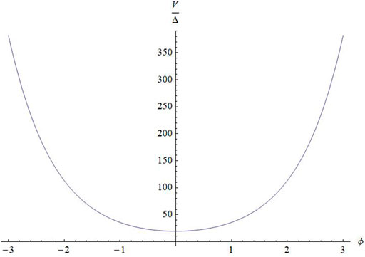
FIGURE 1. V/Δ as a function of ϕ. The γ = 0.237 5 and 8πG = 1 are adapted in the calculation.

Then the resulted Friedman equations read

$\begin{array}{ccc}\hfill H^2& =\hfill & \frac{\kappa }{3}\rho ,\left(b\to 0\right)\hfill \end{array}(41)$

$\begin{array}{ccc}\hfill H^2& =\hfill & \frac{\kappa }{3}\rho ,\left(b\to \frac{\pi }{2}\right)\hfill \end{array}(42)$

which is also a symmetric bounce.

6 Concluding Remarks

To summarize, the loop quantum cosmological model which consists of the purely Lorentzian term is studied in this article. We consider the spatially flat homogeneous FRW model. It turns out that the modified Friedmann equation keeps the same form as the APS LQC model. However, the critical matter density for the bounce point is only a quarter of the previous APS model, that is, ${\rho }_{cL}=\frac{{\rho }_c}{4}$. This is interesting because from Eq. 31, we can see that the strength of quantum gravity becomes significant when $\frac{\rho }{{\rho }_{cL}}\sim 1$, since ρ_cL < ρ_c, in this sense, the lower critical bounce density means the quantum gravity effects will get involved earlier than the previous LQC model. Besides, the lower critical density also means the detection of quantum gravity effects is easier than the previous model. It should be note that in this article, we only consider the cosmological implication of LQC from ADM Hamiltonian which only contains the purely Lorentzian term. However, since the Lorentzian term and the Euclidean term lead to different results at the quantum mechanical level, one can also naturally consider the mixture of these two terms. This of course possible; Assanioussi et al. (2018); Assanioussi et al. (2019); Zhang et al. (2021) show that when we consider the Lorentzian term and the Euclidean term appearing in the Hamiltonian constraint simultaneously, an effective cosmological constant could emerge at the large volume limit.

It should be noted that there are many aspects of the new LQC which deserve further investigating. For example, it is still desirable to the perturbation theory of the new LQC; in this case, the spatial curvature will not be zero. And thus could be inherent more features from the full theory of LQG. Moreover, Yang et al. (2019) adapt an alternative regularization procedure via the Chern–Simons theory which is quite different from the usual regularization method in LQG, and the resulting cosmological evolution is different from the APS LQC model. Hence, it is also interesting to study this regularization under our framework of new LQC. We leave all these interesting topics for future study.

Data Availability Statement

The original contributions presented in the study are included in the article/Supplementary Material; further inquiries can be directed to the corresponding author.

Author Contributions

All authors listed have made a substantial, direct, and intellectual contribution to the work and approved it for publication.

Funding

This work was supported by the NSFC with Grant No. 11 775 082.

Conflict of Interest

The authors declare that the research was conducted in the absence of any commercial or financial relationships that could be construed as a potential conflict of interest.

Publisher’s Note

All claims expressed in this article are solely those of the authors and do not necessarily represent those of their affiliated organizations, or those of the publisher, the editors, and the reviewers. Any product that may be evaluated in this article, or claim that may be made by its manufacturer, is not guaranteed or endorsed by the publisher.

References

Ashtekar, A., Pawlowski, T., and Singh, P. (2006). Quantum Nature of the Big Bang. Phys. Rev. Lett. 96, 141301. doi:10.1103/PhysRevLett.96.141301

PubMed Abstract | CrossRef Full Text | Google Scholar

Ashtekar, A., Bojowald, M., and Lewandowski, J. (2003). Mathematical Structure of Loop Quantum Cosmology. Adv. Theor. Math. Phys. 7, 233–268. doi:10.4310/atmp.2003.v7.n2.a2

CrossRef Full Text | Google Scholar

Ashtekar, A., and Lewandowski, J. (2004). Background Independent Quantum Gravity: A Status Report. Class. Quan. Grav. 21, R53–R152. doi:10.1088/0264-9381/21/15/r01

CrossRef Full Text | Google Scholar

Ashtekar, A. (2009). Loop Quantum Cosmology: an Overview. Gen. Relativ Gravit. 41, 707–741. doi:10.1007/s10714-009-0763-4

CrossRef Full Text | Google Scholar

Ashtekar, A., Pawlowski, T., and Singh, P. (2006). Quantum Nature of the Big Bang. Phys. Rev. Lett. 96, 141301. doi:10.1103/physrevlett.96.141301

PubMed Abstract | CrossRef Full Text | Google Scholar

Ashtekar, A., and Singh, P. (2011). Loop Quantum Cosmology: A Status Report. Class. Quan. Grav. 28, 213001. doi:10.1088/0264-9381/28/21/213001

CrossRef Full Text | Google Scholar

Assanioussi, M., Dapor, A., Liegener, K., and Pawłowski, T. (2018). Emergent de sitter epoch of the quantum cosmos from loop quantum cosmology. Phys. Rev. Lett. 121 (8), 081303. doi:10.1103/PhysRevLett.121.081303

PubMed Abstract | CrossRef Full Text | Google Scholar

Assanioussi, M., Dapor, A., Liegener, K., and Pawlowski, T. (2019). Emergent de Sitter epoch of the Loop Quantum Cosmos: a detailed analysis. Phys. Rev. D 100, 084003. doi:10.1103/physrevd.100.084003

CrossRef Full Text | Google Scholar

Assanioussi, M., Lewandowski, J., and Makinen, I. (2015). New Scalar Constraint Operator for Loop Quantum Gravity. Phys. Rev. D 92, 044042. doi:10.1103/physrevd.92.044042

CrossRef Full Text | Google Scholar

Bojowald, M. (2005). Loop Quantum Cosmology. Living Rev. Relativ. 8, 11. doi:10.12942/lrr-2005-11

PubMed Abstract | CrossRef Full Text | Google Scholar

Dapor, A., and Liegener, K. (2018). Cosmological Effective Hamiltonian from Full Loop Quantum Gravity Dynamics. Phys. Lett. B 785, 506–510. doi:10.1016/j.physletb.2018.09.005

CrossRef Full Text | Google Scholar

Han, M., Ma, Y., and Huang, W. (2007). Fundamental Structure of Loop Quantum Gravity. Int. J. Mod. Phys. D 16, 1397–1474. doi:10.1142/s0218271807010894

CrossRef Full Text | Google Scholar

Rovelli, C. (2004). Quantum Gravity. Cambridge, United Kingdom: Cambridge University Press.

Google Scholar

Thiemann, T. (2007). Modern Canonical Quantum General Relativity. Cambridge, United Kingdom: Cambridge University Press.

Google Scholar

Yang, J., Ding, Y., and Ma, Y. (2009). Alternative Quantization of the Hamiltonian in Loop Quantum Cosmology. Phys. Lett. B 682, 1–7. doi:10.1016/j.physletb.2009.10.072

CrossRef Full Text | Google Scholar

Yang, J., Zhang, C., and Ma, Y. (2019). Loop Quantum Cosmology from an Alternative Hamiltonian. Phys. Rev. D 100, 064026. doi:10.1103/physrevd.100.064026

CrossRef Full Text | Google Scholar

Zhang, X., and Ma, Y. (2011). Extension of Loop Quantum Gravity to F(R) Theories. Phys. Rev. Lett. 106, 171301. doi:10.1103/PhysRevLett.106.171301

PubMed Abstract | CrossRef Full Text | Google Scholar

Zhang, X., Long, G., and Ma, Y. (2021). Loop Quantum Gravity and Cosmological Constant. Phys. Lett. B 823, 136770. doi:10.1016/j.physletb.2021.136770

CrossRef Full Text | Google Scholar

Zhang, X., and Ma, Y. (2011). Extension of Loop Quantum Gravity tof(R)Theories. Phys. Rev. Lett. 106, 171301. doi:10.1103/physrevlett.106.171301

PubMed Abstract | CrossRef Full Text | Google Scholar

Zhang, X., and Ma, Y. (2012). Loop Quantum Brans-Dicke Theory. J. Phys. Conf. Ser. 360, 012055. doi:10.1088/1742-6596/360/1/012055

CrossRef Full Text | Google Scholar

Zhang, X., and Ma, Y. (2011). Nonperturbative Loop Quantization of Scalar-Tensor Theories of Gravity. Phys. Rev. D 84, 104045. doi:10.1103/physrevd.84.104045

CrossRef Full Text | Google Scholar