The Space Physics Environment Data Analysis System in Python

1 Introduction

Dynamically typed, interpreted languages, such as Interactive Data Language (IDL) and Matlab, have exploded in usage for day-to-day data analysis due their ease of use, curated libraries of scientific routines, simplified debugging, and interactive plotting. There is a need for tools tailored toward the Heliophysics community; for example, to provide access to the scientific data from multiple missions in a generic and easy-to-use way, as well as general analysis tools to work with these data. Releasing generic analysis tools has numerous benefits, such as limiting duplication of effort and reducing potential errors made by researchers. In IDL, this need led to the development of the SolarSoft (SSW)¹ package for solar physicists and the Space Physics Environment Data Analysis System [SPEDAS; Angelopoulos et al., 2019)² package for space physicists. The SPEDAS package supports loading, plotting, analysis, and integration of data from several space-based and ground-based observatories, providing a comprehensive environment for space physics data analysis and visualization. While powerful, IDL has numerous limitations, including the high cost of licensing, limited support, difficulty in bridging among different programming languages, as well as conflicts with other libraries caused by the single namespace limitation. The single namespace limitation requires that all IDL functions have unique names, making it nearly impossible to use SPEDAS and other large packages (e.g., SolarSoft) in the same environment without naming conflicts.

Due to these limitations and the increasing popularity of the Python programming language (Burrell et al., 2018), we began the development of an implementation of the IDL SPEDAS package in the Python programming language. The tools in PySPEDAS allow users to access scientific quality data products from numerous space missions and ground observatories with only a few lines of code. PySPEDAS provides a variety of generic analysis tools, from simple operations, such as interpolating magnetic field data, to more complex operations, such as calculating and plotting 2D slices of 3D velocity distribution data from particle instruments.

Development of PySPEDAS is occurring on GitHub at:

https://github.com/spedas/pyspedas

Development of PySPEDAS is occurring in the open to encourage contributions from mission teams as well as the general Heliophysics community.

PySPEDAS releases are distributed using the Python Package Index (PyPI) and can be installed with:

pip install pyspedas

PySPEDAS conforms to the Python in Heliophysics Community standards³. PySPEDAS is platform independent, supporting the Windows, macOS, and Linux operating systems, and is released under a permissive free software license (MIT).

Each function in PySPEDAS is documented in the docstring of that function. The HTML documentation is built automatically from these docstrings using the Sphinx documentation generator⁴. The HTML documentation can be found online at:

https://pyspedas.readthedocs.io/

PySPEDAS examples are available as Jupyter notebooks in general and mission-specific repositories at the SPEDAS GitHub organization⁵. Tutorials are regularly held at scientific meetings, and webinars are regularly held online and are made available on the SPEDAS YouTube channel⁶.

PySPEDAS is tested using standard Python-based unit tests that are automatically ran when code is merged with the master branch. These tests typically exist in the tests directory of each module. While these tests exercise the functionality, they do not typically check the validity of the results. To validate the results, unit tests are implemented in IDL SPEDAS which compare the data products from PySPEDAS to the data products in IDL SPEDAS. These validation tests are released in IDL SPEDAS, as well as in a separate repository at the SPEDAS GitHub organization.

In the next section, we give an overview of the “tplot” model, describe the load routine design, and finally describe several analysis tools currently available.

2 Materials and methods

Internally, PySPEDAS uses the tplot data model to store, manipulate and visualize time series data; in Python, this model is implemented by the PyTplot⁷ project. The tplot data model is an extremely powerful model for working with time series data, with heritage from IDL, that allows users to reference complex data sets, along with their metadata, using simple string identifiers.

2.1 Tplot model

Because of its importance, here we repeat the principles of the tplot data model. In the tplot data model, time series data are stored, alongside metadata, in global objects called tplot variables. The tplot data model is shown in Table 1. The time values are stored as Unix times (number of seconds since 00:00:00 UTC on 1 January 1970, excluding leap seconds) in the x component of the variable. These values should be monotonically increasing. The data values are stored in the y component, error bars are stored in the optional dy component, and additional dependencies (e.g., energy and angular ranges) are stored in the optional v, v1, v2, and v3 components of the variable.

TABLE 1

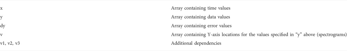
TABLE 1. Tplot data model.

PyTplot provides importers for a variety of file formats, including CDF files, netCDF files, STS files, as well as IDL sav files. These importers use other open-source libraries (e.g., cdflib⁸, netCDF4⁹, scipy¹⁰, astropy¹¹, etc.) to load the data and time values into numpy arrays, then convert the time values to a common epoch (Unix time), and then store the tplot variables containing the time values, data, and metadata, using the name of the variable as a reference.

A suite of PyTplot routines provides an environment for working with tplot variables, e.g., creating variables (pytplot.store_data), plotting those variables (pytplot.tplot), returning the data in numpy arrays or xarray objects (pytplot.get_data), setting figure options (pytplot.tplot_options), setting panel options (pytplot.options), as well as doing basic calculations such as data cropping (pytplot.crop) and data averaging (pytplot.avg_res_data). A list of the tplot variables in the current session can be found using the pytplot.tplot_names function, and the metadata for a variable can be accessed by setting the metadata option when calling (pytplot.get_data). A full list of the routines and their functionality can be found in the PyTplot documentation.

The plotting features provided by PyTplot are extensive, supporting multiple possible backends (including Bokeh, Qt, and matplotlib), each supporting stacked time series plots containing any combination of line and spectrogram panels. In addition to the standard features supported by the Bokeh and Qt backends, the current backend used by PySPEDAS (matplotlib) supports error bars, annotations, highlighting time intervals, automatic spectrogram interpolation, overplotting lines on top of spectrograms, creating figures in Jupyter notebooks, as well as saving publication quality figures.

2.2 Load routines

The instrument load routines in PySPEDAS follow the form:

pyspedas.mission.instrument ()

And implement a common set of keywords for access to the data (as shown in Table 2). Some missions [e.g., Magnetospheric Multiscale (MMS; Burch et al., 2016)] implement additional keywords to provide additional options when loading the data. Each mission implements at least one core load routine, with instrument-specific wrappers implemented as separate functions. The core load routines typically download the data files, load the data files into PyTplot variables, perform common post-processing (e.g., time clipping of the data), then return a list of the variables that were loaded. The instrument-specific functions can then call these core routines to load the data. This model, adapted from IDL SPEDAS, allows for instrument-level pre- and post-processing in the wrapper routines, while most instrument-independent loading is done in a common core routine shared by the instruments. Multiple core routines can be developed for access to different data servers (e.g., one for a mission’s official data server and one for the NASA archive).

TABLE 2

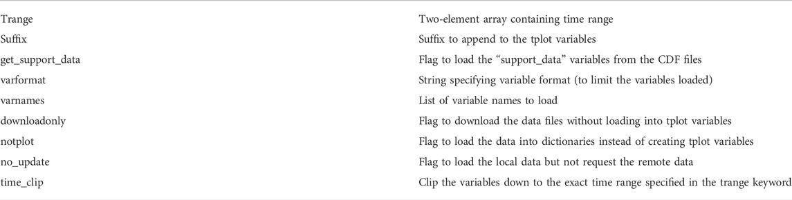
TABLE 2. Standard load routine keywords.

PySPEDAS contains several support routines for downloading data files from remote repositories, including:

pyspedas.dailynames: generates a list of file names from a time range using the strftime format

pyspedas.download: general download routine that uses the open-source requests¹² library internally, supports authentication, allows parsing and searching HTML directory index pages generated by Apache, and provides local caching and file version numbers.

pyspedas.hapi.hapi.hapi: supports loading data from Heliophysics Data Application Programmer’s Interface (HAPI)¹³ servers; uses hapiclient¹⁴ package to load the parameters into numpy arrays, then creates tplot variables.

By default, the data files are stored in a subdirectory of the current working directory; this directory can be changed using the SPEDAS_DATA_DIR environment variable, as well as mission-specific environment variables (e.g., MMS_DATA_DIR for MMS, THM_DATA_DIR for THEMIS). The mission-specific environment variables override the global SPEDAS data directory set in SPEDAS_DATA_DIR. The local data directories can also be changed in the Python interpreter by setting the ‘local_data_dir’ key in the mission’s CONFIG dictionary; e.g., pyspedas.themis.config.CONFIG [‘local_data_dir’] = ‘/path/to/data/’ for THEMIS.

Once the data files are saved locally, the core load routines typically use importers inside PyTplot, described in (Section 2.1), to save the parameters as tplot variables. The wrapper routines then take these loaded variables and do any instrument-specific post-processing (e.g., creating additional data products, applying calibrations and corrections, setting plot metadata, etc.).

Table 3 shows a list of the current projects supported by PySPEDAS as of July 2022.

TABLE 3

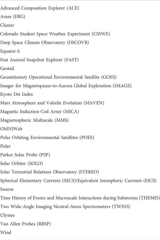
TABLE 3. Projects supported as of July 2022.

2.3 Analysis tools

2.3.1 Coordinate transformations

Coordinate transformations are implemented in the pyspedas.cotrans module. The cotrans function, located in the pyspedas.cotrans module, accepts any tplot variable containing vector data in Cartesian coordinates and supports transformations to and from several coordinate systems (Hapgood 1992): Geocentric Equatorial Inertial (GEI), Geocentric Solar Ecliptic (GSE), Geocentric Solar Magnetospheric (GSM), Solar Magnetic (SM), Geographic (GEO), Geomagnetic (MAG) and Geocentric Equatorial Inertial for epoch J2000.0 (J2000).

Internally, these transformations are direct translations of the IDL SPEDAS coordinate transformation routines, which were originally based on the ROCOTLIB¹⁵ library. In addition to the calculations to perform the various transformations, the pyspedas.cotrans module utilizes the tplot metadata where possible; i.e., if the input coordinate system is stored in the variable’s metadata, the user does not need to specify it manually. The output variable’s metadata are updated to the new coordinate system (including in any plot annotations), minimizing the amount of user effort to produce transformed data with proper annotations.

The pyspedas.cotrans module also provides tools for transforming vector data into various field-aligned coordinate systems (for which the Z axis corresponds to the direction of a given field vector, X and Y axes defining the plane perpendicular to it); pyspedas.cotrans.fac_matrix_make generates field-aligned coordinate transformation matrices, and pyspedas.cotrans.tvector_rotate rotates vector data using these matrices.

In addition to tplot variables, the pyspedas.cotrans module supports data and time inputs as simple numpy arrays. If numpy arrays are provided instead of tplot variables, the pyspedas.cotrans module will create a tplot variable internally prior to performing the transformation.

2.3.2 Magnetic field models

Routines for working with magnetic field models are implemented in the pyspedas.geopack module. Functions are available for generating the Tsyganenko 89, 96, and 2001 models, as well as the Tsyganenko-Sitnov 2004 model at arbitrary points in space (as a function of time) (Tsyganenko, 2013). Internally, these functions extract the input position data from tplot variables, then use the pure-Python implementation of the Geopack library¹⁶ to generate the various field models at each point, then store the results in tplot variables.

The Tsyganenko 96, 2001, and Tsyganenko-Sitnov 2005 models require additional solar wind input. The pyspedas.geopack module contains routines (get_tsy_params, get_w_params) for generating the required input parameters to this model using the OMNI solar wind data loaded using the pyspedas.omni.data function.

2.3.3 Curlometer technique

The curlometer technique is implemented in the pyspedas.analysis.lingradest routine. This function takes position and magnetic field data obtained at four spacecraft (e.g., MMS or Cluster) and applies the linear gradient/curl estimator technique (Dunlop et al., 2021) to calculate the magnetic field gradients, divergence, curl, and field line curvature. This routine is a direct translation of the IDL SPEDAS version originally developed for Cluster (Runov et al., 2003) and most recently used by MMS.

The core lingradest function is called by an MMS-specific wrapper mms_lingradest in the pyspedas.mms.fgm module; this wrapper interpolates the spacecraft position and magnetic field data to the first spacecraft timestamps, then calls the lingradest function to perform the calculations and saves the output in tplot variables.

2.3.4 Dynamic power spectrum

The dynamic power spectrum of a tplot variable can be calculated using the pyspedas.tdpwrspc function. This function extracts the data from the input tplot variables, and then a Hanning window is applied to the input data (its power is divided out of the returned spectrum). A straight line is subtracted from the data to reduce spurious power due to the sawtooth behavior of a background. The output, the mean squared amplitude of the signal at each specific frequency, is then stored in separate tplot variables for each component. Keyword options are available for controlling the number of points to use for the Hanning window, the number of points to shift for each spectrum, and the output frequency bin size. Options are also available for disabling the Hanning window and straight line subtraction.

2.3.5 Wave polarization tools

The pyspedas.twavpol function allows for performing wave polarization analysis of three orthogonal component time series data in tplot variables. This function extracts the data from the input tplot variable, which usually has been moved into a magnetic field-aligned coordinate system such that wave angle and ellipticity refer to the magnetic field direction. It then passes the input data to a core wavpol routine (Samson and Olson, 1980), which calculates the degree of polarization, wave normal angle, ellipticity, and helicity, then saves the output in tplot variables. The wave polarization tools in PySPEDAS are direct translations of the IDL SPEDAS routines for performing the same calculations.

2.3.6 Particle tools

General (mission independent) particle tools are implemented in the pyspedas.particles module, with mission-specific particle tools implemented in the particles submodule of a mission’s module (e.g., MMS particle tools are implemented in pyspedas.mms.particles). Tools exist for taking particle data structures and calculating the energy, theta, phi, pitch angle, and gyrophase spectrograms, as well as plasma moments of velocity distribution functions. In addition, tools exist for calculating and plotting 2D slices of the velocity distribution functions.

The PySPEDAS particle data structure, which is based on the IDL data structure, is shown in Table 4. The units_name attribute of the particle data structure must be counts, rate, eflux, flux, df, df_cm, df_km, e2flux, or e3flux. For the theta and phi values, the PySPEDAS particle tools use presumed particle trajectories (not look direction of the instrument).

TABLE 4

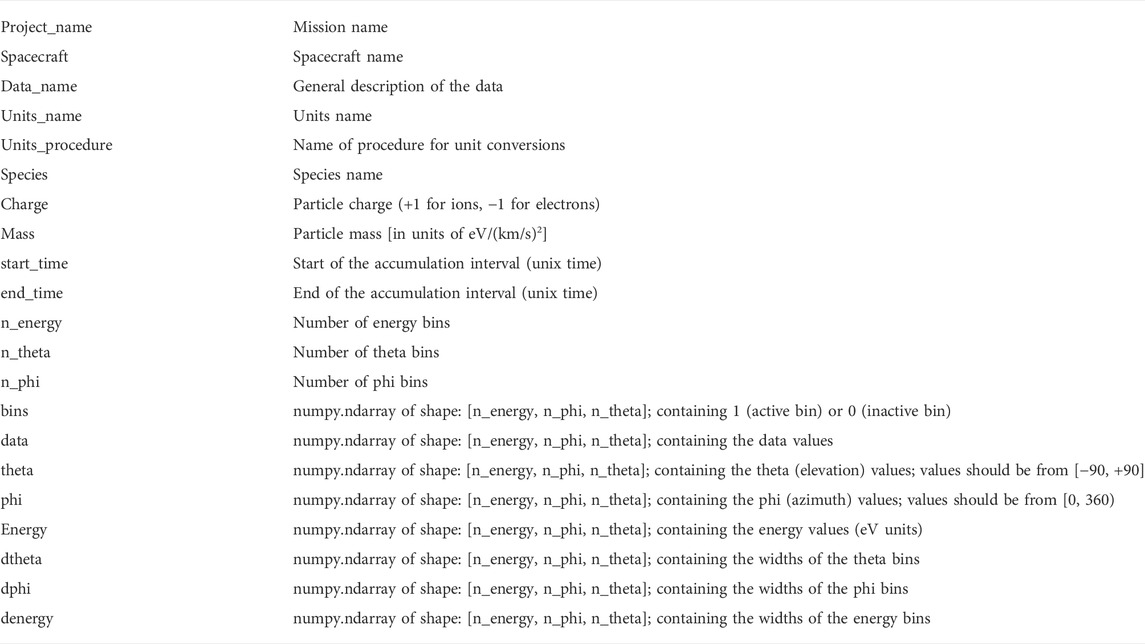
TABLE 4. The particle data structure.

The user-facing functions for doing particle calculations can be found in the particles submodule of the mission’s module, e.g., spectrograms and moments for MMS can be calculated using the mms_part_getspec function found in the pyspedas.mms.particles module. This function loads particle distribution function data (as well as any required support data), re-forms the data into the standard PySPEDAS particle data structure described above, then uses various generic functions to perform the calculations, and stores the output as tplot variables. Options exist for changing the species, limiting the energy and angular ranges, changing the output units, disabling internal and external electron photoelectron corrections [for the Fast Plasma Instrument (FPI; Pollock et al., 2016)], and more.

Slices of MMS distribution function data can be plotted using the mms_part_slice2d function, also found in the pyspedas.mms.particles module. Just as above, this function loads the data and any required support data, creates the PySPEDAS particle data structures, then uses generic tools to calculate and plot the slice. Options exist for rotating the slice into a variety of coordinate systems, limiting the energy range, changing the interpolation type, smoothing, and more.

2.3.7 Spherical elementary currents/equivalent ionospheric currents plots

The pyspedas.secs module allows for downloading and plotting vector and contour maps of Spherical Elementary Currents and Equivalent Ionospheric Currents data (Weygand et al., 2011). The data are downloaded from the Virtual Magnetospheric Observatory¹⁷ using pyspedas.secs.data, and the data are plotted using the make_plots function in the pyspedas.secs.makeplots module. Internally, this function uses matplotlib to create the figures.

3 Results

3.1 Basic example

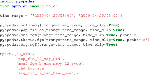
Figure 1 shows magnetic field data measured by five spacecraft, including Solar Orbiter, Parker Solar Probe, MMS, THEMIS, and Arase, for 2 h on 20 April 2020. Using PySPEDAS, the data for this figure can be loaded with a total of two imports, five function calls, one for each instrument, and the figure can be plotted with a sixth function call, e.g., Figure 1 can be re-created using the following:

FIGURE 1

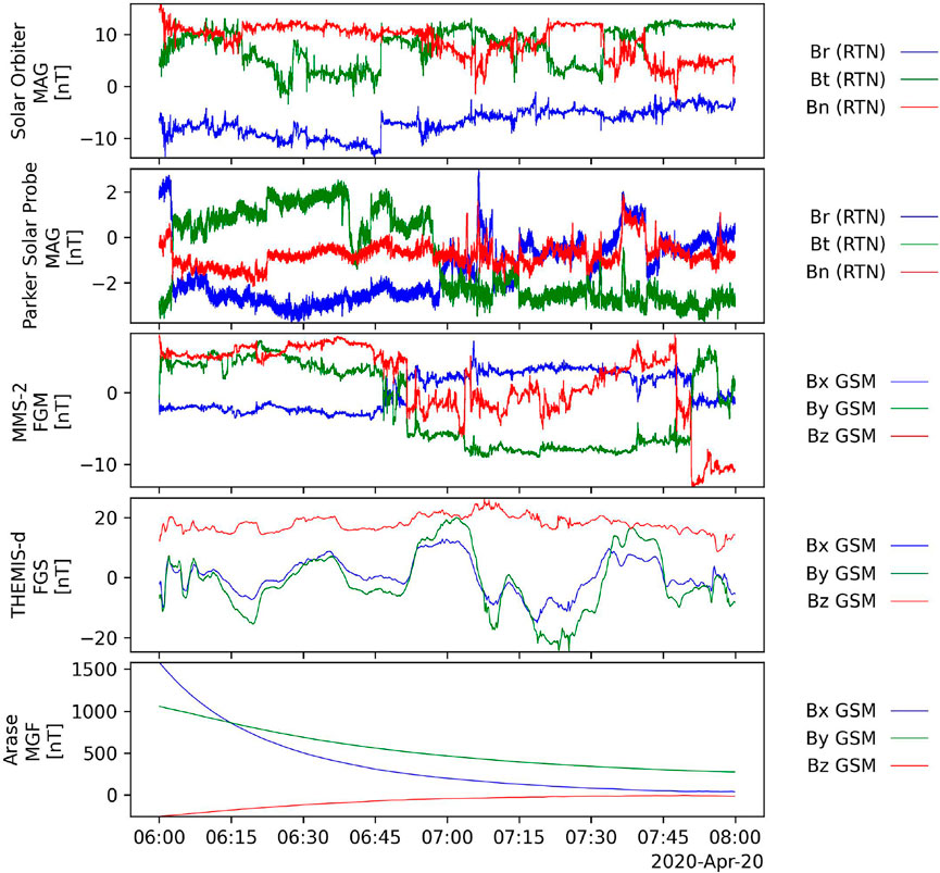
FIGURE 1. Magnetic field data from Solar Orbiter, Parker Solar Probe, Magnetic Multiscale Mission, THEMIS, and Arase missions for 2 h on 20 April 2020.

Algorithm 1. Graph construction.

Each load routine call returns a list of the variable names that were loaded, and users are encouraged to review the mission team’s documentation for details on the loaded data products.

The tools (load and analysis routines) shown in these examples have additional options that can be found in the docstrings (available in the interpreter by calling the help function with the PySPEDAS function as an argument), as well as in our online documentation.

In this example, as well as several of those that follow, we made minor adjustments to some of the figure annotations prior to saving (using pytplot.options) for consistency; the full code for generating all figures can be found in the Supplementary Material.

3.2 Post-processing example

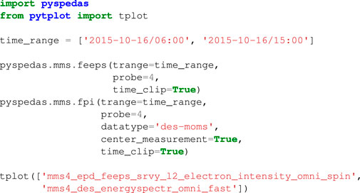
Figure 2 shows fast survey electron data from the Fast Plasma Investigation (FPI) and Fly’s Eye Energetic Particle Sensor (FEEPS; Blake et al., 2016) instruments onboard MMS-4 on 16 October 2015.

FIGURE 2

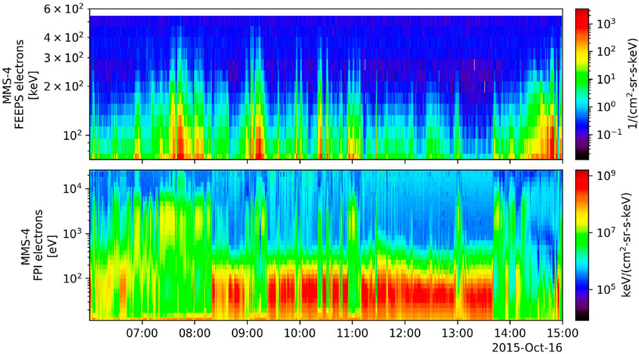
FIGURE 2. Electron energy spectra observed by the (A) Fly’s Eye Energetic Particle Sensor (FEEPS) and (B) Fast Plasma Investigation (FPI) instruments on 16 October 2015.

Each measurement is taken over a certain time interval, called the accumulation interval, when data were acquired for that measurement. The FPI measurements are stored at the beginning of the accumulation interval, while other instruments (e.g., FEEPS) are stored at the middle of the accumulation interval; in order to correct this, the user must center the FPI measurements using the center_measurement option in the FPI load routine.

The FEEPS spin-averaged omni-directional data shown in Figure 2 are calculated after the individual telescope data are loaded from the CDF files. These data have numerous corrections applied in post-processing prior to calculating the omni-directional data products, including flat field corrections (for ions), energy table corrections, bad and inactive telescope removal, and sunlight contamination removal.

Algorithm 2. Figure 2 can be re-created using the following:

3.3 Coordinate transformation example

Figure 3 shows 2 h of MMS FGM and Arase MGF (Matsuoka et al., 2018) data on 20 April 2020. The first panel shows the MMS-2 FGM data in GSE coordinates, loaded from the CDF file, and the second panel shows the MMS-2 data transformed from GSM coordinates. The third and fourth panels of Figure 3 show the Arase MGF data in GSE coordinates, loaded from the CDF file, and the Arase MGF data, in GSE coordinates, transformed from GSM. In both cases, the transformed data matches the GSE data loaded from the CDF files.

FIGURE 3

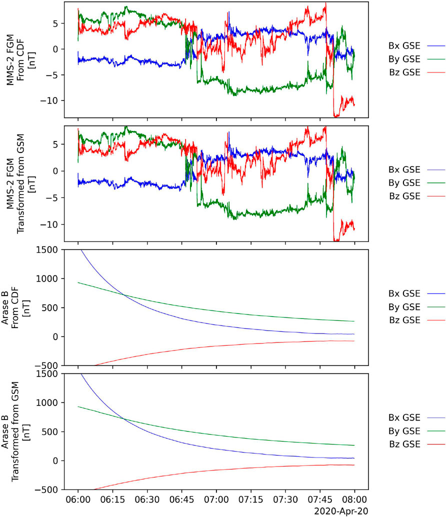
FIGURE 3. From top to bottom, (A) FGM data observed by MMS-2 in GSE coordinates (from the CDF files), (B) MMS-2 FGM data in GSE coordinates transformed from GSM coordinates, (C) Arase MGF data in GSE coordinates (from the CDF files), and (D) Arase MGF data in GSE coordinates transformed from GSM coordinates.

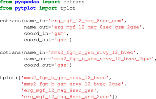
Algorithm 3. Figure 3 can be re-created using the following:

3.4 Magnetic field model example

Figure 4 shows a comparison of the measured magnetic field at the Arase and THEMIS spacecraft and the magnetic field model produced by the Tsyganenko 89 model at each spacecraft location on 20 April 2020. The spacecraft position and magnetic field data can be loaded in two function calls per spacecraft, and the Arase position data can be converted to kilometers from Earth radii using pyspedas.tkm2re in a single function call. The T89 model can be calculated at each position data with another function call per spacecraft, and the results can then be plotted with one final function call.

FIGURE 4

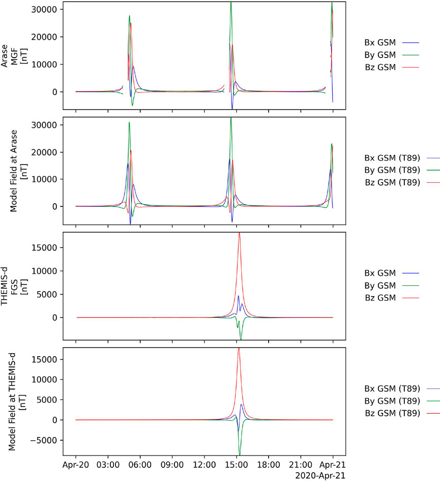
FIGURE 4. From top to bottom, (A) Arase MGF data (GSM coordinates), (B) T89 model field at the Arase position (GSM coordinates), (C) THEMIS-d FGS data (GSM coordinates), and (D) T89 model field at the THEMIS-d position (GSM coordinates).

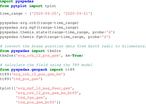
Algorithm 4. Figure 4 can be re-created using the following:

3.5 Curlometer example

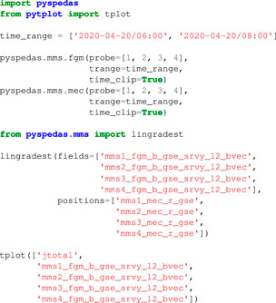
Figure 5 shows the magnetic field in GSE coordinates measured by all four MMS spacecraft on 20 April 2020 (bottom four panels) and the total current calculated using the linear gradient descent curlometer technique using the field and spacecraft position (MMS Ephemeris/Coordinates; MEC) data for each probe (top panel). The data can be loaded in two function calls, the curlometer calculations require only another function call, and the results can be plotted using a final function call.

FIGURE 5

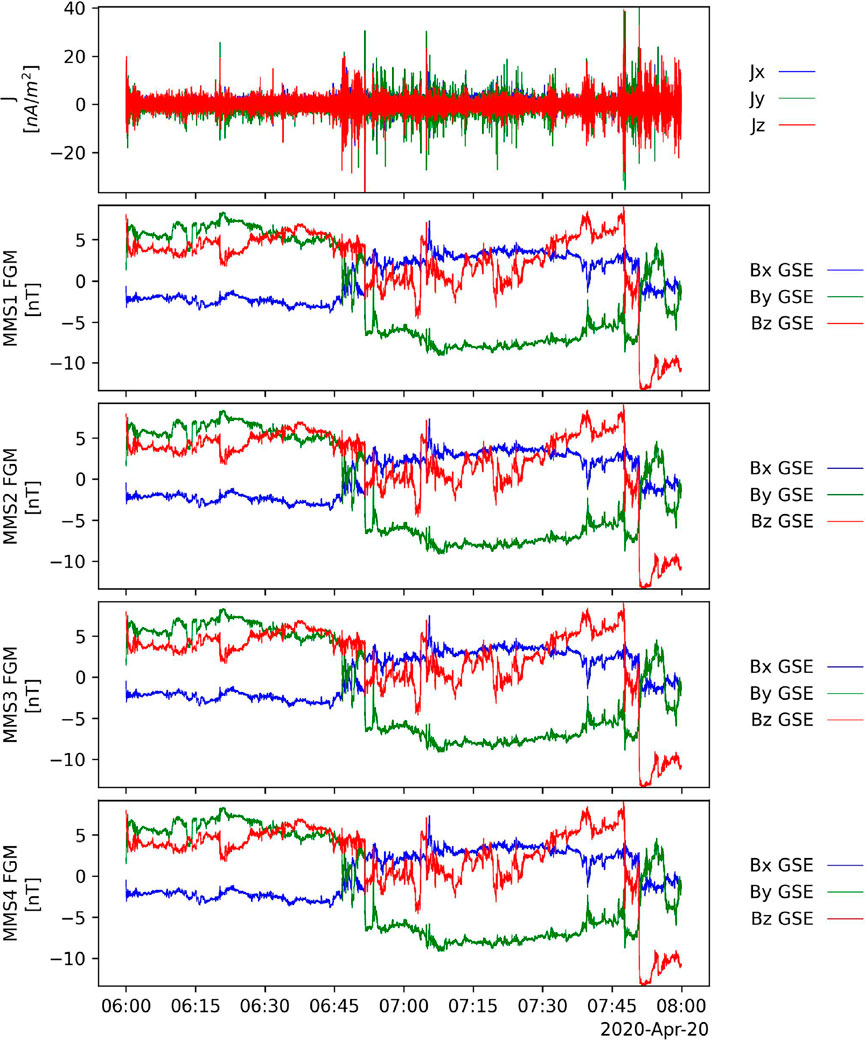
FIGURE 5. From top to bottom, (A) the current density from the curlometer technique, (B) MMS-1 FGM data (C) MMS-2 FGM data (D) MMS-3 FGM data (E) MMS-4 FGM data (all GSE coordinates).

Algorithm 5. Figure 5 can be re-created using the following:

3.6 Dynamic power spectrum example

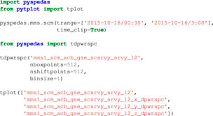
The top panel of Figure 6 shows the fast survey AC magnetic field [(0.5, 16 Hz) frequency range] measured by the Search Coil Magnetometer (SCM) instrument onboard MMS for 3 h on 16 October 2015. The bottom three panels show the X, Y, and Z components of the dynamic power spectra of the SCM data in the top panel. The dynamic power spectra were calculated using a Hanning window of 512 points and 512 points to shift for each spectrum. The data can be loaded with a single function call, the dynamic power spectra can be calculated using another function call, and the results can be plotted with a final function call.

FIGURE 6

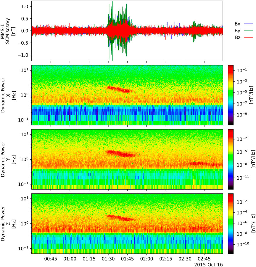
FIGURE 6. From top to bottom, (A) MMS-1 survey mode SCM data (GSE coordinates), dynamic power spectra of the (B) X component, (C) Y component, (D) Z component.

Algorithm 6. Figure 6 can be re-created using the following:

3.7 Wave polarization example

The top panel of Figure 7 shows the SCM data from Figure 6 transformed into magnetic field-aligned coordinates. The next panels show the wave power, degree of polarization, wave normal angle, ellipticity, and helicity calculated using the SCM data shown in Figure 6. If one component is an order of magnitude greater than the other two, then the polarization results saturate and erroneously indicate high degrees of polarization at all times and frequencies. The script to recreate this example would take multiple pages, so it is provided as a separate file in the Supplementary Material.

FIGURE 7

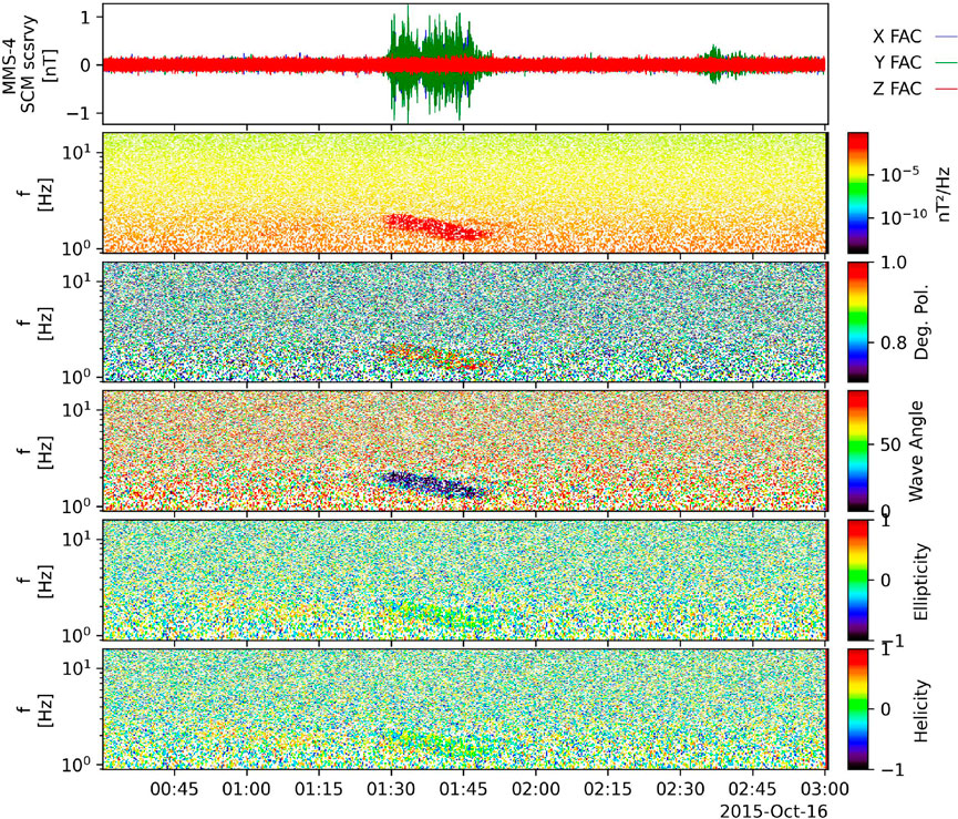
FIGURE 7. From top to bottom, (A) MMS-1 survey mode SCM data (field-aligned coordinates, (B) wave power, (C) degree of polarization, (D) wave angle, (E) ellipticity, (F) helicity.

3.8 Velocity distribution function example

Figure 8 shows a comparison of the ion density and energy spectra calculated using mms_part_getspec with those released by the FPI team in CDFs for 2 h on 16 October 2015.

FIGURE 8

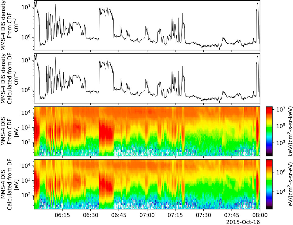
FIGURE 8. From top to bottom, (A) MMS-4 DIS number density (from CDF files), (B) MMS-4 DIS number density [calculated from the distribution function (DF) data], (C) MMS-4 DIS energy spectra (from CDF files), (D) MMS-4 DIS energy spectra (calculated from the DF data).

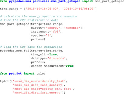
Algorithm 7. Figure 8 can be re-created using the following:

3.9 2D Slice of distribution function example

Figure 9A shows a 2D slice of FPI ion distribution data produced with the mms_part_slice2d. The figure shows a field-aligned, bi-directional beam of 0–300 eV ions observed by FPI onboard MMS-1 at 09:32:19 UT on 10 September 2017. The energy range was limited to 0–300 eV, and the data were rotated such that the x-axis is parallel to the magnetic field and the bulk velocity defines the x-y plane. The slice was calculated using “geometric” interpolation, i.e., each point on the plot is given the value of the bin it intersects.

FIGURE 9

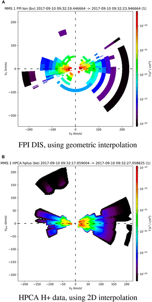
FIGURE 9. 2D slices showing a bi-directional beam of 0–300 eV ions observed by MMS-1 (A) FPI DIS, rotated such that x-axis is parallel to the magnetic field and the bulk velocity defines the x-y plane. (B) HPCA H+, rotated such that the B x V (bulk) vector defines the x-y plane.

Figure 9B shows a 2D slice of HPCA H+ distribution data produced with the mms_part_slice2d for the same event as above. The energy range was limited to 0–300 eV, but in this case, the data were rotated such that the B x V (bulk) vector defines the x-y plane, and the slice was calculated using 2D interpolation instead of geometric. Using the 2D interpolation method, data points within the specified theta or z-axis range are projected onto the slice plane and linearly interpolated onto a regular 2D grid.

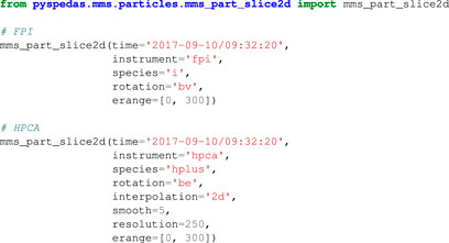
Algorithm 8. This figure can be re-created using the following:

3.10 Spherical elementary currents/equivalent ionospheric currents example

Figure 10A shows the Spherical Elementary Currents, and Figure 10B shows the Equivalent Ionospheric Currents (left) at 08:38 UT on 29 February 2008, which can be utilized to investigate the ionospheric currents, and the magnetosphere-ionosphere coupling process, such as the ionospheric response to the magnetospheric substorms.

FIGURE 10

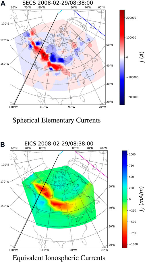
FIGURE 10. Maps showing (A) Spherical Elementary Currents and (B) Equivalent Ionospheric Currents at 08:38 UT on 29 February 2008. The contour map of ionospheric currents reveals a westward electrojet event, which is likely related to magnetospheric activities such as a substorm.

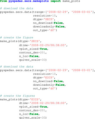
Algorithm 9. This figure can be re-created using the following:

4 Discussion

The examples in the previous section show how powerful PySPEDAS is for Heliophysics research; for each example, the data can be downloaded and plotted in less than a page of code.

We plan to add support for additional projects, datasets, and analysis tools, as well as additional post-processing to several of the projects we currently support. As of July 2022, the tools for working with particle distribution function data are limited to the MMS FPI and HPCA instruments. We are planning on extending support to the particle instruments onboard THEMIS and Arase in the near future. We are also currently implementing tools for minimum variance analysis calculations. In addition to these analysis tools, we plan to add a Graphical User Interface (GUI) and a “calc” mini-language for working with tplot variables, much like those that exist in IDL SPEDAS [see Angelopoulos et al., 2019 for more].

Data availability statement

The datasets presented in this study can be found in online repositories. The names of the repository/repositories and accession number(s) can be found in the article/Supplementary Material.

Author contributions

BH contributed to the development of cdflib, PyTplot, as well as the MAVEN plug-in. NH and AD contributed to the development of various PySPEDAS routines. JL and VA provided program leadership. XCa and XCh contributed the SECS/EICS plug-in. TH, SM C-WJ, SN, MK, TS, and YM contributed the Arase plug-in. OL is the Lead Co-I of the MMS SCM instrument, and contributed significantly to the original dynamic power spectra and wave polarization IDL code and examples.

Funding

The core SPEDAS team acknowledges support from NASA contract NNG17PZ01C (for SPEDAS community support) to UCLA, contract NNG04EB99C (as subcontract from SwRI for MMS SPEDAS plug-in development) to UCLA, and contract NAS5-02099 (THEMIS support of TDAS maintenance and SPEDAS infrastructure) to UCB, UCLA, and BU.

Acknowledgments

We would like to acknowledge the developers of the PyTplot, numpy, cdflib, netCDF4, hapiclient, astropy, and requests packages, as well as Sheng Tian for the geopack package.

Conflict of interest

The authors declare that the research was conducted in the absence of any commercial or financial relationships that could be construed as a potential conflict of interest.

Publisher’s note

All claims expressed in this article are solely those of the authors and do not necessarily represent those of their affiliated organizations, or those of the publisher, the editors and the reviewers. Any product that may be evaluated in this article, or claim that may be made by its manufacturer, is not guaranteed or endorsed by the publisher.

Supplementary material

The Supplementary Material for this article can be found online at: https://www.frontiersin.org/articles/10.3389/fspas.2022.1020815/full#supplementary-material

Footnotes

¹http://www.lmsal.com/solarsoft

²http://www.spedas.org/

³https://heliopython.org/docs/

⁴https://www.sphinx-doc.org

⁵https://github.com/spedas

⁶https://www.youtube.com/channel/UCZVyhCNPI3II7Mu086KsoLA

⁷https://github.com/MAVENSDC/PyTplot

⁸https://github.com/MAVENSDC/cdflib

⁹https://github.com/Unidata/netcdf4-python

¹⁰https://scipy.org/

¹¹https://www.astropy.org/

¹²https://requests.readthedocs.io/

¹³https://hapi-server.github.io/

¹⁴https://github.com/hapi-server/client-python

¹⁵http://cdpp.irap.omp.eu/index.php/services/scientific-librairies/rocotlib

¹⁶https://github.com/tsssss/geopack

¹⁷http://vmo.igpp.ucla.edu/

References

Angelopoulos, V., Cruce, P., Drozdov, A., Grimes, E. W., Hatzigeorgiu, N., King, D. A., et al. (2019). The space physics environment data analysis system (spedas). Space Sci. Rev. 215, 9. doi:10.1007/s11214-018-0576-4

PubMed Abstract | CrossRef Full Text | Google Scholar

Blake, J. B., Mauk, B. H., Baker, D. N., Carranza, P., Clemmons, J. H., Craft, J., et al. (2016). The fly’s eye energetic particle spectrometer (feeps) sensors for the magnetospheric multiscale (mms) mission. Space Sci. Rev. 199, 309–329. doi:10.1007/s11214-015-0163-x

CrossRef Full Text | Google Scholar

Burch, J. L., Moore, T. E., Torbert, R. B., and Giles, B. L. (2016). Magnetospheric multiscale overview and science objectives. Space Sci. Rev. 199, 5–21. doi:10.1007/s11214-015-0164-9

CrossRef Full Text | Google Scholar

Burrell, A. G., Halford, A., Klenzing, J., Stoneback, R. A., Morley, S. K., Annex, A. M., et al. (2018). Snakes on a spaceship—An overview of python in heliophysics. J. Geophys. Res. Space Phys. 123. doi:10.1029/2018JA025877

CrossRef Full Text | Google Scholar

Dunlop, M. W., Dong, X.-C., Wang, T.-Y., Eastwood, J. P. S. H., Yang, Y.-Y., Haaland, S., et al. (2021). Curlometer technique and applications. JGR. Space Phys. 126. doi:10.1029/2021JA029538

CrossRef Full Text | Google Scholar

Hapgood, M. (1992). Space physics coordinate transformations: A user guide. Planet. Space Sci. 40, 711–717. doi:10.1016/0032-0633(92)90012-D

CrossRef Full Text | Google Scholar

Matsuoka, A., Teramoto, M., Imajo, S., Kurita, S., Miyoshi, Y., and Shinohara, I. (2018). The mgf instrument level-2 high-resolution magnetic field data of exploration of energization and radiation in geospace (erg) arase satellite. doi:10.34515/DATA.ERG-06000

CrossRef Full Text | Google Scholar

Pollock, C., Moore, T., Jacques, A., Burch, J., Gliese, U., Saito, Y., et al. (2016). Fast plasma investigation for magnetospheric multiscale. Space Sci. Rev. 199, 331–406. doi:10.1007/s11214-016-0245-4

CrossRef Full Text | Google Scholar

Runov, A., Nakamura, R., Baumjohann, W., Treumann, R. A., Zhang, T. L., Volwerk, M., et al. (2003). Current sheet structure near magnetic x-line observed by cluster. Geophys. Res. Lett. 30, 1579. doi:10.1029/2002GL016730

CrossRef Full Text | Google Scholar

Samson, J. C., and Olson, J. V. (1980). Some comments on the descriptions of the polarization states of waves. Geophys. J. Int. 61, 115–129. doi:10.1111/j.1365-246X.1980.tb04308.x

CrossRef Full Text | Google Scholar

Tsyganenko, N. A. (2013). Data-based modelling of the earth’s dynamic magnetosphere: A review. Ann. Geophys. 31, 1745–1772. doi:10.5194/angeo-31-1745-2013

CrossRef Full Text | Google Scholar

Weygand, J., Amm, O., Viljanen, A., Angelopoulos, V., Murr, D., Engebretson, M. J., et al. (2011). Application and validation of the spherical elementary currents systems technique for deriving ionospheric equivalent currents with the north American and Greenland ground magnetometer arrays. J. Geophys. Res. 116. doi:10.1029/2010JA016177

CrossRef Full Text | Google Scholar