pyDARN: A Python software for visualizing SuperDARN radar data

1 Introduction

The Super Dual Auroral Radar Network (SuperDARN) is an international network of more than 30 high frequency (HF, 3–30 MHz) coherent scatter radars that provide continuous, coordinated observations of the electrodynamics of the Earth’s upper atmosphere from middle to polar latitudes (Greenwald et al., 1995). The radars detect coherent backscatter from decameter-scale electron density irregularities which act as tracers for the large-scale plasma circulation in the F-region ionosphere. The radars also detect backscatter from meteor plasma trails at around 90 km altitude, and backscatter from the ground or sea surface, which occurs when the transmitted radio waves undergo total internal reflection by the ionosphere and then scatter on the ground/sea. These three types of backscatter (ionospheric, ground/sea, meteor) can be used for studying the ionospheric signatures of a wide range of phenomena including plasma convection, high latitude plasma structures, gravity waves, magnetohydrodynamic waves, and substorm processes (Chisham et al., 2007; Nishitani et al., 2019, and references therein).

As with many geophysical datasets, effective and accessible data visualization tools are essential for enabling scientists to use the data. The SuperDARN community has a long history of developing and sharing data visualization tools among SuperDARN institutions and with the wider space physics community, which is described further in Section 3. However, the software needs of data users change over time and the dataset appears to present a number of challenges to new users. One of the major challenges is that SuperDARN produces several types of multidimensional data products, and these are stored using a highly-customized file format that cannot easily be read using common scientific analysis software. Furthermore, many of the common methods for visualizing SuperDARN data require additional data preparation or assumptions that are standard within the SuperDARN community but are not necessarily obvious to other users, such as the reflection height assumptions required for assigning geographic coordinates to a scattering target (Chisham et al., 2008). While these challenges are distinct from data visualization, they present significant barriers to non-expert users who want to use SuperDARN as a supporting dataset in their scientific work.

To make SuperDARN data more accessible to the wider space physics community, the SuperDARN community has developed a new open-source Python3 library for SuperDARN data visualization called pyDARN (SuperDARN Data Visualization Working Group et al., 2022). This new library provides a user-friendly way to visualise SuperDARN data in all the ways that have become standard in the SuperDARN scientific community, including time series plots, range-time plots, field of view plots, scan plots, and global convection maps. pyDARN is maintained on GitHub (https://github.com/SuperDARN/pydarn) by the SuperDARN Data Visualization Working Group (DVWG), which includes volunteer members from many institutions. The package is licensed under the GNU Lesser General Public License version 3 (https://www.gnu.org/licenses/lgpl-3.0.en.html). In this paper, we review the different types of SuperDARN data products, pyDARN’s development history and goals, the current structure and functionality of the software, and future development plans. We provide examples demonstrating how the current implementation of pyDARN makes it easy for students, researchers, and other interested individuals to access, visualize, and analyze different SuperDARN data products. We believe that pyDARN as a Python software tool will help advance space science by making the SuperDARN dataset accessible to a broader scientific community.

2 SuperDARN data products

SuperDARN radars operate in the 8–20 MHz frequency range. Each radar consists of a linear array of antennas that are phased electronically to produce a steerable beam that is narrow in azimuth $(\sim 5°)$ and wide in vertical extent $(\sim 40°)$. This beam is divided into 70–110 range gates which are 45 km wide in the standard operational mode. Depending on the number of beams and range gates used, the total field of view covers a 52–78° azimuthal sector that extends to 3,500–5,000 km in range. This allows the radars to detect coherent backscatter from scattering targets over a very wide geographical area, including two-dimensional observations from pairs of radars with overlapping fields of view. In addition to the main antenna array, most SuperDARN radars have a smaller ‘interferometer’ array of antennas that is displaced by about 100 m from the main array, and this is used to determine the angle-of-arrival (elevation angle) of the backscatter returns. The radars transmit sequences of unevenly-spaced pulses, and the returns from 20 to 30 sequences obtained during the standard ∼3 s dwell time are averaged together before further analysis. In the standard operational mode, a complete scan of all 16–24 beams is completed every minute. When the data from multiple radars are combined to produce convection maps, the standard time resolution of the data product is 2 min.

The primary data products of SuperDARN are power (signal-to-noise ratio), Doppler velocity, and spectral width. For radars with an interferometer array, the elevation angle of the received backscatter can also be calculated after careful calibration (Chisham et al., 2021). These data products are determined in a two-stage process commencing with the level-zero-type data product consisting of the in-phase and quadrature (I&Q) samples measured by the receiver for each multipulse sequence. These samples are then processed into a complex-valued autocorrelation function (ACF) for each range gate along the sampling beam. These ACFs are the ‘raw’ data product that are distributed to the scientific community, as described in the Data Availability Statement. The power, velocity, spectral width and elevation angle in each range gate are then determined using a program called FitACF, which is one of the core routines in the standard SuperDARN data analysis software, the Radar Software Toolkit (RST) (SuperDARN Data Analysis Working Group et al., 2022). This software also includes routines for combining the line-of-sight (LoS) velocity measurements from individual radars onto a hemispheric grid of equal-area cells, and for applying a global fitting technique called Map Potential to determine the global convection pattern (Ruohoniemi and Baker, 1998).

SuperDARN data are stored using a self-describing file format called ‘DataMap’ (DMap). This file format was developed to suit the operational environment of the radar sites, including encoding the real-time data stream provided by some radars. A description of the data fields included in each format is included in the RST documentation (https://radar-software-toolkit-rst.readthedocs.io/en/latest/). The DMap files have a different structure depending on the type of data stored, and they are named as follows:

• *.iqdat: I&Q voltage samples, named IQDat file

• *.rawacf: Raw autocorrelation functions, named RawACF file

• *.fitacf: Fitted parameters including power, Doppler velocity, spectral width, elevation angle, and their errors, named FitACF file.

• *.grid/*.grd: Fitted parameters from all radars in one hemisphere placed on a grid of equal-area cells spanning 1° of geomagnetic latitude, named Grid file.

• *.map: Contains the same data as *.grid files, as well as the fitted coefficients describing the convection pattern, named Map file.

Note that prior to 2006, SuperDARN data were stored in a binary data format, and these files cannot currently be read using the Python tools described in this paper. However, the RST includes routines for converting these binary files to the DMap format so that they can be used in pyDARN.

In addition to the data formats above, the SuperDARN community maintains set of text files containing basic technical information about each radar that is required for data analysis and visualization. These ‘hardware files’ include information such as the radar location, scanning boresight direction, the number of beams and the beam separation. These files are stored in a GitHub repository (https://github.com/SuperDARN/hdw) and pyDARN can automatically access them as required.

3 pyDARN development

3.1 History

Data visualisation tools have been shared within the international SuperDARN community since the early years of the collaboration. Early versions of the RST (then known as radops) were primarily used for processing of the radar data on-site, with basic plotting functionality included for range-time-intensity (RTI) and field-of-view (FOV) plots. This code, however, could not handle non-standard radar operating modes or coordinate systems beyond rectilinear. In an effort to expand SuperDARN plotting functionalities and to make it more flexible for the growing SuperDARN user base, S. Milan at the University of Leicester led the development of a dedicated SuperDARN data visualisation software package called Go in the early 2000s. Go was written in the Interactive Data Language (IDL), which was the most commonly used programming language in the community at the time. As a result, Go became popular throughout the SuperDARN community and received contributions from numerous scientists from many institutions.

In 2009, a postdoctoral fellow at Virginia Tech, L. Clausen, developed Go into a new IDL package, the Data Visualisation Toolkit (DaViT). Over time, research students at Virginia Tech added new analysis and visualisation tools to the package including HF raytracing (de Larquier et al., 2013a), total electron content (TEC) maps overlayed with SuperDARN data (Thomas et al., 2013), and data diagnostics. DaViT also included the THEMIS Data Analysis Software (TDAS, http://themis.igpp.ucla.edu/software.shtml, see also Angelopoulos et al. (2019)) for downloading space- and ground-based data from the THEMIS mission. This allowed users to plot THEMIS all-sky imager data overlaid with radar data (e.g., Gallardo-Lacourt et al., 2014). The DaViT source code was distributed online, and it was also used to run a suite of online data visualisation tools on the Virginia Tech SuperDARN website (http://vt.superdarn.org). These widely-used online visualisation tools are connected to a SuperDARN data server at Virginia Tech, allowing anyone in the world to generate plots of SuperDARN data from any time period since late 1993.

In 2012, the growing popularity of the Python language in the space physics community prompted research students at Virginia Tech to port DaViT from IDL to Python2, creating a new package called DaViTPy (de Larquier et al., 2013b). This effort was led by S. de Larquier, A. J. Ribeiro, and N. A. Frissell. DaVitPy’s place among other space physics Python packages is described in Burrell et al. (2018). The package was developed collaboratively on Github, which facilitated code contributions from the wider scientific community and allowed development to continue after the original developers graduated. DaViTPy provided FTP access to the Virginia Tech data server, so the data necessary for producing a particular plot could be downloaded automatically. Python tools for performing coordinated studies with incoherent scatter radars and satellite missions, as well as Python wrappers for various Fortran-based models and analysis routines (IGRF, AACGM, NRLMSISE, HWM, IRI, and HF raytracing) were also added to DaVitPy. The SuperDARN data visualisation tools, the provision of processed SuperDARN data (FitACF, Grid, and Map files) via the Virginia Tech data server, and the integration with other space physics software and models in DaVitPy led to a substantial increase in the use of SuperDARN data in the wider space physics community.

By 2018 it was apparent that DaVitPy had become challenging to maintain due to its broad scope, and the package had a long list of dependencies that made it difficult for users to install. The planned deprecation of Python2.7 at the beginning of 2020 also provided the impetus to review the package structure and scope while transitioning to Python3. At the same time, the SuperDARN Principal Investigators decided that processed SuperDARN data (FitACF, Grid, and Map) would no longer be distributed, instead favouring a citable archive of the raw data that users must process themselves with the RST. While this was a necessary step to support scientific reproducibility, this decision has created an extra barrier for users who must now install the RST and work through multiple steps of data analysis before they can visualise the data. All of these factors led to a community decision to deprecate DaVitPy and develop a new package in Python3 that would focus solely on SuperDARN data visualisation. DaVitPy was officially deprecated and archived in 2020 (Ribeiro et al., 2020).

The pyDARN project was then initiated at the University of Saskatchewan, with M. Schmidt and M. Detwiller as the lead developers of the data visualisation code and the I/O code respectively. Development began in 2018 and the first official release was published in March 2020 (Detwiller et al., 2020).

3.2 Development goals

pyDARN is developed with four primary goals in mind: usability, accessibility, maintainability and flexibility. These goals, or objectives that would fall within these goals, are often used when describing programming ‘best practices’. For example, in the list of good Python design principles of PEP 20 The Zen of Python (Tim Peters, 2004), tenets such as ‘Readability counts’ (accessibility), ‘If the implementation is hard to explain, it is a bad idea’ (usability, maintainability) and ‘Sparse is better than dense’ (flexibility) are included. pyDARN’s goals are upheld during development through extensive code review and unit testing.

For usability, it is vital that pyDARN is easy to download, install and use. The pyDARN software package is listed on PyPi, making it easy to install from any Linux or Mac terminal using pip: pip install pydarn. pyDARN functions can then be accessed in the same way as other popular software packages. For example, the ‘Maps’ and ‘RTP’ modules can be imported using: from pydarn import Maps, RTP. Complete examples are provided in the accompanying Jupyter notebook. PyDARN now includes all of the standard SuperDARN data visualisation types, and these are described further in Section 5. The pyDARN developers seek user feedback on new features as part of the code review process, and welcome new code contributions and other input from the scientific community. However, since pyDARN relies on scientists and engineers volunteering their time to contribute to the package, requests for new functionalities can only be accommodated if someone is willing to volunteer their time to develop them.

SuperDARN data visualisation often requires additional analysis tools to prepare the data for plotting. These include determining the distance (slant range) to the backscatter, projecting the field of view onto geographic coordinates, and performing coordinate transforms. Therefore, pyDARN includes a wide range of functions that are not directly related to plotting. These functions are not typically called by users, but will be called by the plotting code in an ‘under-the-hood’ fashion. For example, pyDARN includes several virtual height models (e.g., Chisham et al., 2008) that are an essential part of assigning geographic coordinates to the backscatter. In all cases, the standard virtual height model that is most widely accepted by the SuperDARN community is called by default if no model is specified by the user. This greatly improves pyDARN’s ease of use and accessibility for non-expert users and for those who wish to quickly view the data before fine-tuning the results later.

pyDARN is developed in a way that allows for simple maintainability and expansion. Code is modularized as much as possible to avoid duplicating functionality across multiple different modules and methods. For example, fan, grid and convection map plots all share access to methods that generate map projections, radar FOV locations, and Python colour maps, meaning that any bug fixes can be applied without needing to consider the intricacies of all the functions that call them.

Expansion of capability is also very important for pyDARN. SuperDARN users may wish to build upon existing functionality, or add new features entirely, so pyDARN must be designed in such a way that code changes or expansions are easy to achieve. For example, new plotting map projections can be developed directly into the separate module dedicated to projections. pyDARN methods that already use projections can then use the new projections immediately without any further code modification, as they already contain a call to the ‘projections’ enumeration members. Similarly, new virtual height models for geolocating data can be appended into the corresponding module, making it available for range and coordinate estimations. More information about the layout and structure of pyDARN’s code can be found in Section 4.

Finally, pyDARN is flexible such that users can easily integrate and overlay data from non-SuperDARN sources, such as from satellites or ground-based instruments. Plots are returned as regular Matplotlib axis objects with their inherent ability to be customised. In addition, data and their corresponding coordinates can also be returned to be utilised in any Python plotting code.

3.3 Workflow and testing

To achieve the goals described in Section 3.2, the pyDARN development team has a published workflow and testing regime, which is described fully in the documentation. The team uses Pull Requests and Code Reviews, requiring that at least two developers approve the code to maintain standards. Anyone is welcome to develop in pyDARN, and the team fosters a welcoming and inclusive environment though a code of conduct.

At present the library has users on Windows, MacOS, openSUSE, CentOS, Ubuntu, and many other Linux operating systems. In general, all new components are tested on Windows, MacOS and at least one Linux based system. The majority of our new users are based in Windows, and many of the developers use MacOS, but users based in operations rather than research use numerous Linux systems and as such pyDARN is required to be system-independent.

4 Structure and components

pyDARN is structured as an application containing several internal packages. The structure of the current version, pyDARN 3.0 (SuperDARN Data Visualization Working Groupet al., 2022), is illustrated in Figure 1. There are three top-level directories: pydarn, docs and test. The pydarn directory contains the main codebase that is shipped and installed for users. The remaining top-level directories are containers for the documentation and the testing suite.

FIGURE 1

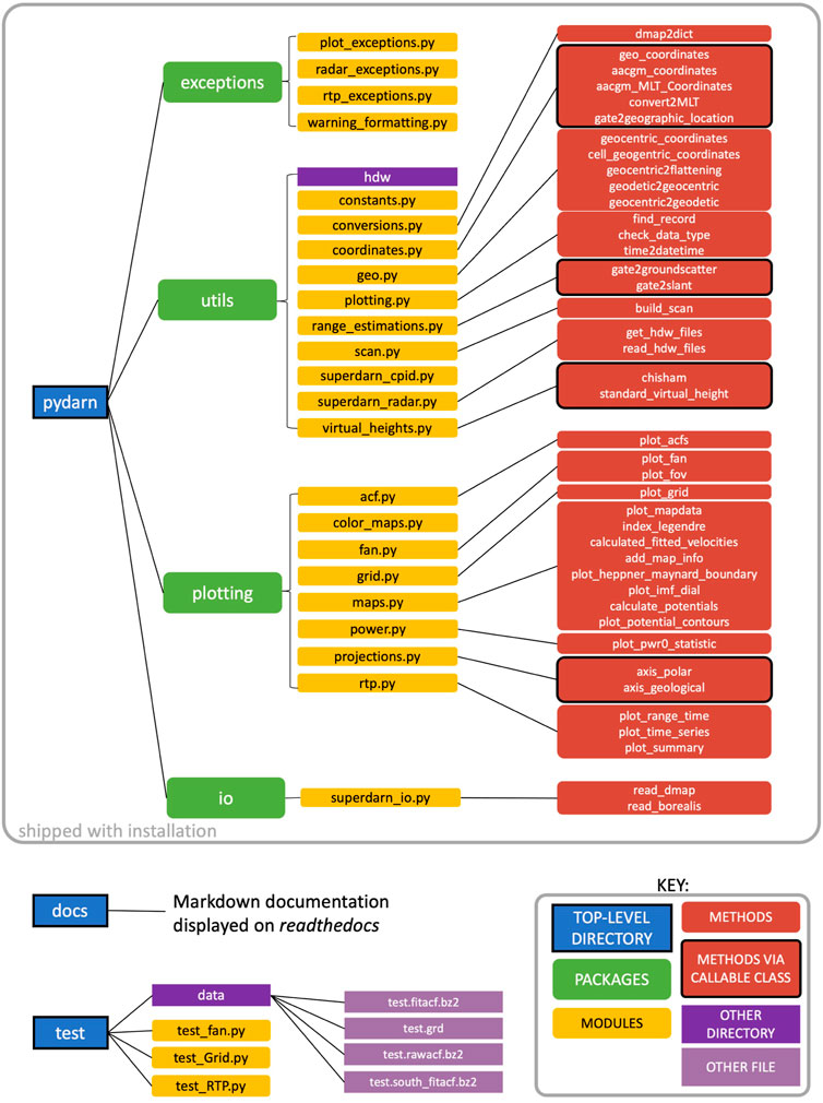
FIGURE 1. Layout and structure of the pyDARN v3.0.0 library, including the packages, modules and some of the more commonly used methods that are shipped with the installation. Also shown are other peripheral directories that are useful in development and discussion.

4.1 Main codebase

The pydarn directory contains four packages. There are three main packages used for data visualisation, and an additional package, exceptions, which provides useful warnings and troubleshooting information that might be required to visualise a particular dataset. The exceptions are grouped into modules relating to generic plotting, specific types of plots, reading data files, and accessing radar hardware information. In addition, the team uses warnings to advise the user that optional dependencies are not installed, or that the data file is not suitable for plotting in the requested format. For example, a warning message is also displayed on import to remind the user to cite pyDARN in published work.

The central package in the pyDARN library is the plotting package. This package allows the user to visualise SuperDARN data in all the formats that have become standard in the SuperDARN scientific community (see Section 2), such as range-time plots and convection maps. Each type of visualisation has its own module, and examples are provided in Section 5. The plotting directory also contains two utilities modules, color_maps.py and projections. py, which provide special color maps developed especially for SuperDARN data visualisation, and polar or Cartesian matplotlib axis objects, respectively. Note that for any plotting function with a color bar, the color map can also be customized by changing the cmap parameter.

The utils package provides a range of utilities that support the plotting package. Some modules are merely used for storing physical constants (constants.py) or dictionaries for storing radar control program information (superdarn_cpid.py). Other modules contain methods that are essential to plotting, such as determining the geocentric coordinates of each cell in the radar field of view (geo.py), and organising the data into ‘scans’ (scan.py) so that a sequence of observations covering the entire azimuthal field of view can be visualised as a ‘fan’ plot (see Section 5). These modules replicate similar routines available in the RST. A number of modules (coordinates.py, range_estimations.py and virtual_heights.py) are used as callable classes, where the user selects an option in the plotting method call, which then automatically selects the chosen method from the module. For example, the virtual_heights.py module includes two virtual height models that can be used for mapping the location of backscatter targets in the ionosphere (Chisham et al., 2008). A class within the virtual_heights.py module will be called and this option will be entered into the module, and the corresponding virtual height model, Standard or Chisham, will be used. This design allows the user to easily select virtual height models, slant range estimates for ionospheric or ground scatter, and geographic or geomagnetic coordinate systems for use in any compatible plotting method. It also allows for greater flexibility and extensibility in development, since additional options, models or coordinate systems can be added and integrated with ease.

The utils package also includes the superdarn_radar.py module, which is designed to retrieve, update and format information about each SuperDARN radar that is required for data visualisation such as the radar location, the direction of the centre beam (boresight), and the dates of operation. This information is provided by each radar’s Principal Investigator though the SuperDARN hardware files repository on GitHub (https://github.com/SuperDARN/hdw). Upon installation of pyDARN, the hardware repository is copied from GitHub and placed within the library under the utils package. The user can update the hardware files to the latest version at any time using get_hdw_files, which re-installs the hardware files from source. The hardware file contents can be read using read_hdw_files, which formats the data into a class object. The superdarn_radar.py module also contains general information about each radar, including the full name, 3-letter station code, and the name and institution of the principal investigator. The superdarn_radar.py module is designed to work outside of the data visualisation and will provide hardware information to the user through the SuperDARNRadars class. Further information and examples are given in Section 5 and the Jupyter notebook.

4.2 Documentation

To enhance the usability of the pyDARN library, extensive documentation and tutorials are written for each module. These are updated for each version release and can be found at https://pydarn.readthedocs.io/en/main/. The documentation is written in Markdown and built using MkDocs. To increase the accessibility, usability and flexibility of the code, the team uses standard PEP8 styling for the codebase. This styling is checked frequently using the flake8 library (Cordasco, 2022). The NumPy docstring convention is used to document modules, methods, and classes within the codebase. This helps the developers maintain the codebase and makes it easier for new developers to join the team.

4.3 Testing suite

The testing suite, found in the GitHub repository, is not included in the library at installation and is only used for development purposes. It allows the developers to determine whether a change to the codebase has altered or broken any of the library’s functionality. The testing suite uses pytest (Krekel et al., 2022) and checks for multiple different inputs to each of the plotting methods. These tests can be performed by cloning the repository and running pytest in the top-level directory, which will run all of the tests within the directory at once.

4.4 Dependencies

pyDARN has several dependencies that are required to use the library. When installing with pip, the pyDARN setup will check that all dependencies are installed and update them if necessary. pyDARN currently requires Python version 3.6 or higher and the following packages to be installed: pyDARNio version 1.1.0 or higher (SuperDARN Data Standards Working Group et al.,2022), AACGMv2 (Burrell et al., 2021), Matplotlib version 3.3.4 or higher (Hunter, 2007), PyYAML (Simonov, 2021), and NumPy (Harris et al., 2020). pyDARNio requires that the h5py (Collette, 2008), deepdish (Larsson, 2021) and pathlib2 (Troffaes, 2022) libraries are installed. Finally, Cartopy (Met Office, 2010–2015) is an optional dependency of pyDARN that is used for displaying coastlines on some types of plots.

4.4.1 The IO package and pyDARNio

pyDARNio is an open source Python library for reading, writing and reformatting SuperDARN data. pyDARNio provides read support for the standard SuperDARN DMap data format and the HDF5-format files produced by the Borealis digital radar system (SuperDARN Canada, 2022). It also contains methods to write HDF5-format files and convert them to the DMap format.

pyDARNio was originally developed as an internal package of pyDARN. However, it was found that the IO sections of code were very useful for other Python-based SuperDARN software, including the Borealis radar control system which was developed alongside. Therefore, pyDARNio was separated from pyDARN to create a light-weight IO package that could be integrated into other packages that did not require the data visualisation tools in pyDARN. As a result, pyDARNio is now a dependency for pyDARN, and it is automatically installed during the pyDARN installation. Methods within pyDARNio are called by pyDARN’s internal io package without the user having to import pyDARNio separately. The io package copies the pyDARNio method SDarnRead and converts it to SuperDARNRead in pyDARN, allowing all DMap files including IQDat, RawACF, FitACF, Grid, and Map files to be read by pyDARN.

Besides enabling data to be read for plotting purposes, pyDARNio has some additional functionalities for reading the HDF5-format Borealis data and compressing time-sequenced data into large arrays. This reduces the file size and allows the data to be read quickly. The pyDARNio package therefore serves the greater purpose of providing read and write support for a larger set of SuperDARN filetypes like those used in Borealis. The modularization of the Python file manipulation functions for SuperDARN into the pyDARNio package constrains all file-related tasks to a single package.

4.4.2 Altitude-Adjusted Corrected Geomagnetic and other coordinate systems

pyDARN produces a range of azimuthal projection plots that use either geographic or geomagnetic coordinate systems. Fan plots are produced from FitACF files using a projection of the radar FOV onto a geographic or geomagnetic coordinate system. The method for determining the geographic coordinates of each range–beam cell in the FOV is included in geo.py. This is a translation from the original cnvtcoord.c procedure in the RST that was written in C by K. Baker, R.J. Barnes and D. Andre. These geographic coordinates are then converted into geomagnetic coordinates depending on the input parameters used to produce the fan plot. The data in Grid and Map files are given in geomagnetic coordinates, and pyDARN does not perform any coordinate transformations when generating grid plots or convection maps. Therefore, these plots cannot currently be produced in geographic coordinates.

The geomagnetic coordinate system used is version two of the Altitude-Adjusted Corrected Geomagnetic (AACGM) coordinate system (Shepherd, 2014). The forward and inverse transformations between geographic and AACGM coordinates are performed using the AACGMv2 Python library (Burrell et al., 2021), which is a Python wrapper for the AACGM-v2 C library (Shepherd, 2019). This library also calculates magnetic local time (MLT), which is commonly used in SuperDARN azimuthal plots instead of magnetic longitude. Example conversions between geographic and AACGM coordinates are available in the Burrell et al. (2021) documentation.

4.4.3 Cartopy (optional)

Cartopy is a Python package for processing geospatial data (Met Office, 2010–2015). In pyDARN it is used to plot the outlines of the continents in fan plots, grid plots and map plots (see Section 5). At present, the implementation in pyDARN is available only when plotting in geographic coordinates, where a return of the ax object allows the ax.coastlines() option to be used. The next minor release of pyDARN will allow coastlines from Cartopy to be plotted in geomagnetic coordinates as well. In the future, the coastlines option will be integrated into the projections.py module for use with all geospatial plotting as a keyword rather than an addition to the axis.

The installation process for Cartopy is more complicated than the other pyDARN dependencies due to different requirements for each operating system and some users may prefer a more streamlined version. Therefore, pyDARN does not install Cartopy by default and instead directs users to the Cartopy installation instructions at https://scitools.org.uk/cartopy/docs/latest/. If a user attempts to use a Cartopy-dependent method without installing Cartopy, pyDARN will raise an exception and display a message in the terminal window.

5 Functionalities

This section provides examples of pyDARN’s primary and auxiliary functionalities and descriptions of scientific analysis that can be done using these plotting functions. Detailed documentation on pyDARN installation and all functionalities mentioned below can be found at https://pydarn.readthedocs.io/en/latest/.

5.1 Primary functionalities

In this subsection we provide examples of various functions for reading SuperDARN data files, and for generating different types of data visualizations including the time series plots, range-time parameter plots, FOV and fan plots, grid plots, and convection plots. The code required to reproduce each plot is provided in the accompanying Jupyter notebook, and information about accessing the underlying data is given in the Data Availability Statement.

5.1.1 Reading SuperDARN files

pyDARN reads SuperDARN data files through the IO package pyDARNio as described in Subsection 4.4.1. pyDARN reads SuperDARN data from the DMap files as follows:

Import pydarn

File = “path/to/file”

SDarn_Data = pydarn. SuperDARNRead (file).

This puts the contents of the file into a Python object called SDarn_data. Then the user will need to specify the type of SuperDARN data that was provided, e.g.

Fitacf_data = SDarn_Data.read_fitacf ()

Rawacf_data = SDarn_Data.read_rawacf ()

Map_data = SDarn_Data.read_map ()

Grid_data = SDarn_Data.read_grid ()

Iqdat_data = SDarn_Data.read_iqdat ()

It is also possible to read DMap files without knowing the file type using read_dmap, as shown in the example below. The resulting variable is a Python dictionary. This function also demonstrates the ability to stack the object creation and data reading into one line of code:

Dmap_data = pydarn. SuperDARNRead (). read_dmap (file).

SuperDARN RawACF and FitACF files usually contain 2 h of data and the files are compressed for distribution using Bzip2 (Seward, 2010). Therefore, multiple input files are required to produce some types of plots. Examples of generic SuperDARN file reading, opening multiple FitACF data files and combining them into one variable for plotting are provided in the Jupyter notebook in the plotting function demonstrations.

In addition to SuperDARN data files, pyDARN can also be used to access radar and hardware information and obtain coordinates for radar FOV. The function pydarn. read_hdw_file can extract radar hardware data based on the 3 letter abbreviation of the radar (e.g., ‘sas’ for the Saskatoon radar). The pydarn. Coords.GEOGRAPHIC and pydarn. Coords.AACGM functions provide easy ways to obtain the coordinates of a specific radar’s FOV in geographic and AACGM coordinates. Examples on accessing radar and hardware information are also provided in the Jupyter notebook.

5.1.2 Time-series plots

Time-series plots are simple line plots of a single fitted parameter from a specific beam and range gate. The parameters that can be plotted are shown in Table 1. Figure 2 shows an example of the time series plot for the LoS velocity parameter from beam 12 and gate 13 of the Prince George (PGR) radar on 25 January 2016 at 00:00–02:00 UT. Clear signatures of ultra-low frequency (ULF) waves are present during this time interval as reported by Shi et al. (2018).

TABLE 1

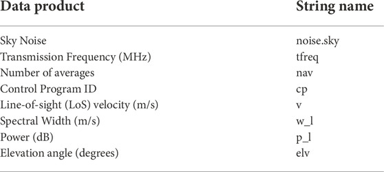
TABLE 1. Commonly used data product and the corresponding string name in SuperDARN DMap files.

FIGURE 2

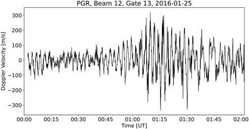
FIGURE 2. Doppler velocity time series from beam 12 and gate 13 of the Prince George radar at 00:00–02:00 UT on 25 January 2016.

5.1.3 Range-time parameter plots

Range-Time Parameter (RTP) plots, also known as range-time-intensity (RTI) plots, are two-dimensional representations of one fitted parameter plotted as a function of range and time for a specific beam. This is the most common way of viewing data from a single radar. The plotting function plot_range_time includes the keyword ‘parameter’ that allows the user to specify which parameter from Table 1 will be plotted. This is specified using the doc string names shown in the second column, and the possible choices are LoS velocity (v), spectral width (w_l), elevation angle (elv), and power (p_l). By default, the velocity parameter is plotted.

Figure 3 shows a RTP plot from beam two of the Clyde River radar when the beam is looking from dawn to dusk at 08:00–10:30 UT on 18 December 2017. Positive (negative) velocities indicate motion towards (away from) the radar. As shown by the arrows (added manually after the figure is generated using pyDARN), there are several sequential flow structures that are moving towards the radar location. These structures correspond to dawnward return flows of the auroral forms resulting from the flux transfer events reported by Hwang et al. (2020).

FIGURE 3

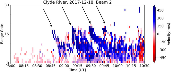
FIGURE 3. Range-time-parameter (RTP) plot of the line-of-sight velocity from beam two of the Clyde River radar at 08:00–10:30 UT on 18 December 2017. Arrows show ionospheric signatures of flux transfer events.

pyDARN provides several ways to modify the vertical axis by specifying the keyword range_estimation. SuperDARN radar beams usually have 75 range gates of length 45 km. In order to have range gates on y axis, range_estimation = pydarn.RangeEstimation.RANGE_GATE can be used. We can also convert the range gates numbers into a slant range in kilometres using range_estimation = pydarn.RangeEstimation.SLANT_RANGE. Ground Scatter Mapped Range is another option that utilizes ground scatter to improve the slant range estimations (Bristow et al., 1994). This can be done by using range_estimation = pydarn.RangeEstimation.GSMR.

5.1.4 Summary plots

Summary plots allow the user to generate a set of RTP plots in which the backscatter is colour-coded by the power (p_l), velocity (v), spectral width (w_l) and, if available, the elevation (elv). This type of plot is useful when more than one parameter is needed to interpret the data, for example to distinguish between ionospheric scatter and ground scatter based on the Doppler velocity and spectral width. The plots also include the sky noise (noise.sky), transmission frequency (tfreq), the number of multipulse sequences transmitted during the dwell time (‘Nave’, see Section 2), and the control program identification number (CPID), which provide an overview of the operational parameters during the time interval.

An example summary plot is shown in Figure 4. This plot shows data from beam 15, channel one of the Hankasalmi SuperDARN radar on 13 February 2014. The top three panels show the summary information described above. The remaining four panels are RTP plots where the backscatter is colour-coded in turn by signal-to-noise ratio (SNR), Doppler velocity, spectral width and elevation. In the velocity panel, a positive velocity indicates motion towards the radar (blue shift) and a negative velocity indicates motion away from the radar (red shift). Backscatter classified as ground scatter using criteria defined in the RST are shaded grey in this panel.

FIGURE 4

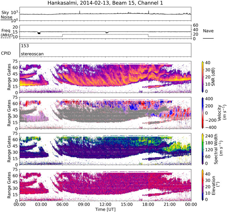
FIGURE 4. Summary plot for beam 15 of the Hankasalmi SuperDARN radar showing power, velocity, spectral width and elevation angle parameters on 13 February 2014.

Several features can be identified in this plot based on the power, velocity and spectral width of the backscatter. A wide band of 1-hop ground scatter spanning more than 30 range gates is present from about 05:00 UT to 20:00 UT. This population of backscatter has been marked as ground scatter using grey shading in the velocity panel. This backscatter population exhibits striations in the SNR associated with F-region electron density perturbations caused by atmospheric gravity wave activity (cf. Samson et al., 1990). At ranges beyond the 1-hop ground scatter is a population of 1.5-hop ionospheric scatter that can be distinguished from the ground scatter based on the higher velocity and spectral width values. A smaller population of 1.5-hop ionospheric scatter is also present in range gates 55–65 at 00:00–03:00 UT. Backscatter from the 0.5-hop propagation mode is detected in gates 15–30 at 00:00–04:00 UT, and also from 20:00 UT onwards. In this latter population, the Doppler velocity oscillations are evidence of ULF wave activity (cf. Ponomarenko et al., 2003). Although elevation angle measurements can be useful for identifying different propagation modes in SuperDARN data, the elevation angle data for this time period appear to be unreliable. If desired, this panel can be removed from the plot by setting plot_elv = False.

5.1.5 Field of view and fan plots

FOV plots show the scanning region of specific radar(s) given the radar station ID. This method provides options for plotting colored FOVs, boundary lines, the radar locations, and labelling the radar names, as well as plotting in different coordinate systems (geographic, AACGM, and MLT). To actually visualize the data from a full radar scan, Fan plot should be used. Fan plot supports the four parameters: velocity (v), spectral width (w_l), power (p_l) and elevation (elv).

Figure 5A shows the FOV of the Saskatoon radar in geographic coordinates where Cartopy has been used to display the coastlines. Figure 5B shows the spectral width data from the Saskatoon (SAS) and Prince George (PGR) radars at 20:08 UT on 1 November 2012 in MLT coordinates. The region of high spectral width values (yellow tiles in Figure 5B) are associated with particle precipitation in the cusp region (cf. Baker et al., 1995). Therefore, the boundary where the spectral width transitions from low to high values indicates the equatorward edge of the particle precipitation region, or equivalently the open close field line boundary (Chisham and Freeman, 2003).

FIGURE 5

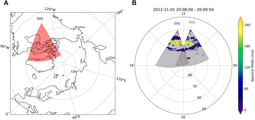
FIGURE 5. FOV plot (left) for the Saskatoon radar and fan plot (right) for the Saskatoon and Prince George radars at 20:08 UT on 1 November 2012.

5.1.6 Grid plots

Grid data is a highly processed data product derived from FitACF data, which has been used with various models to calculate ionospheric electric fields and Joule heating rates (e.g., Matsuo et al., 2021; Wu and Lu, 2022). The LoS vectors are mapped within the cells of an equal-area grid, which is defined in the geomagnetic coordinates system with each cell measuring 1° in latitude, to eliminate biases that would derive from the much denser sampling over nearer radar range gates. The vectors contributed by a radar to a particular cell are averaged over a fixed period of time to obtain the Grid LoS data product. More details of Grid data processing can be found in Ruohoniemi and Baker (1998). The Grid plotting function is suitable for visualizing the combined data from multiple radars. This function can be used to plot the following gridded parameters: gridded LoS velocity, power, and spectral width in AACGM coordinate system. Figure 6 shows an example of a gridded velocity map with good data coverage in the northern hemisphere at 09:20–09:22 UT on 17 March 2015.

FIGURE 6

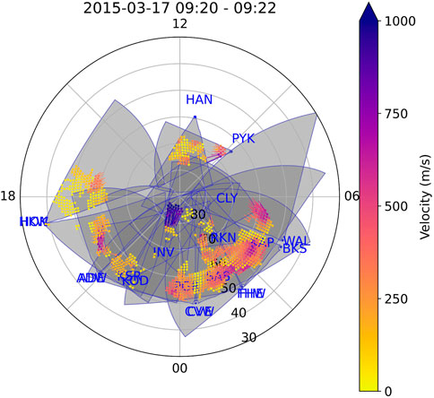
FIGURE 6. Gridded velocity map derived from multiple northern hemisphere radars at 09:20–09:22 UT on 17 March 2015.

5.1.7 Convection map plots

SuperDARN Map files are produced from the combined Grid data and contain the fitted coefficients from a statistical convection model describing the ionospheric convection pattern. Historically, different techniques have been developed to fit the gridded LOS velocities with various background statistical models (Ruohoniemi and Baker, 1998; Cousins et al., 2013; Thomas and Shepherd, 2018). Common parameters in a MAP file that can be plotted by pyDARN is summarized in Table 2.

TABLE 2

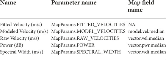
TABLE 2. Common parameters in a MAP file that can be plotted by pyDARN.

The default plotting parameter of a Map file is the fitted velocity, which represent the fitted convection pattern. Another velocity that can be plotted is the modeled velocity, which is the velocity median of the model vectors from a statistical background model (e.g., Thomas and Shepherd, 2018). Other plotting parameters include the raw velocity, power, and spectral width, which are the weighted average velocity, power, and spectral width within every equal-area MLAT/MLON grid cell, respectively. Figure 7 shows an example of the fitted velocity in the northern hemisphere 05:06–05:08 UT on 10 March 2015. The Jupyter notebook contains further examples of plotting options such as color-coded potential contours and convection pattern from the southern hemisphere.

FIGURE 7

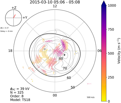
FIGURE 7. Ionospheric convection map with color-coded fitted velocities at 05:06–05:08 UT on 10 March 2015.

5.1.8 Other plots

pyDARN also provides functions to plot auto-correlation functions and statistics of parameters from RawACF files. Specifically, the function pydarn.ACF.plot_acfs plots the real and imaginary parts of the auto-correlation function from a RawACF file for the specified beam and range gate. The function pydarn.Power.plot_pwr0_statistic applies a statistical function (e.g., the mean using numpy. mean) to the lag-0 power for each range/record and plots the results from all records as a function of time. This is a useful function to analyze background radio interference. Examples on how to use these functions can be found in the provided Jupyter notebook and pyDARN documentation.

5.2 Auxiliary functions

In addition to primary functionalities, pyDARN also offers some auxiliary functions to support SuperDARN data analysis. Note that the two functions described below are still under development and are not part of pyDARN as of now. Thus, Figure 8 and Figure 9 cannot currently be produced using pyDARN.

FIGURE 8

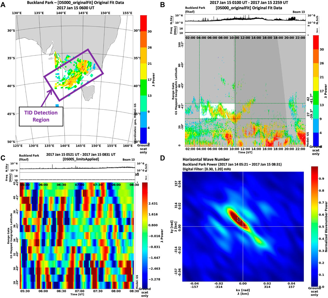
FIGURE 8. Selected outputs from an analysis conducted with the Tholley and Frissell (2022) MUSIC package using ground scatter power observations from the Buckland Park (BPK) SuperDARN radar made on 15 January 2017. (A) Fan plot of one scan of raw data using Ground Scatter Mapped Range estimation. The band of ground scatter where the TID can be detected is indicated by a purple box. (B) RTP plot with times and ranges selected for TID processing highlighted in white. (C) RTP plot showing data interpolated in space and time and filtered with a T = 14 − 56 min bandpass filter. (D) Final wavenumber array indicating the presence of TIDs observed in the radar data. Distance from the origin indicates wavelength, with shorter wavelengths farther away from the origin. Clockwise angle relative to the +y axis indicates propagation direction relative to geographic North. The hotspot marked 1 has a horizontal wavelength λ_h ≈ 890 km, horizontal phase speed v_h ≈ 430 m s⁻¹ propagation azimuth ϕ_azm ≈ − 45°, and period T ≈ 35 min.

FIGURE 9

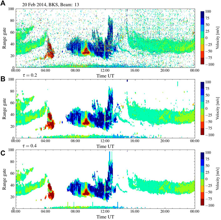
FIGURE 9. RTP plots showing SuperDARN Blackstone radar LoS velocity observations from beam 13 (A) without filtering and filtered using different weights (B) τ = 0.2, and (C) τ = 0.4 on 20 February 2014.

5.2.1 MUSIC for traveling ionospheric disturbances parameter estimation

Traveling Ionospheric Disturbances (TIDs) are quasi-periodic variations in ionospheric electron density that propagate horizontally with time. Medium Scale TIDs (MSTIDs) have periods of ∼15–60 min, horizontal wavelengths of several hundred kilometers, and horizontal phase speeds of ≲ 300 m s⁻¹ (e.g., Ogawa et al., 1987; Samson et al., 1990). MSTIDs may be associated with atmospheric gravity waves (AGWs) (e.g., Hines, 1960; Bristow et al., 1994) or electrodynamic processes (e.g., Kelley, 2011; Atilaw et al., 2021) and therefore are important for understanding atmosphere-ionosphere-geospace coupling. MSTIDs propagating through a SuperDARN radar FOV cause concave and convex structures in the bottomside ionosphere that focus and de-focus HF radio waves returning to the ground, causing the bands of ground scatter detected by the radar to move with time (Samson et al., 1989; Samson et al., 1990; Frissell et al., 2014; Frissell et al., 2016). The ground scatter band movement caused by TIDs also has implications for the operation of terrestrial HF communications systems (Frissell et al., 2022).

In order to measure the wave parameters (i.e., period, horizontal wavelength, phase speed, and propagation direction) of TIDs moving through a SuperDARN FOV, Samson et al. (1990) first implemented the MUltiple SIgnal Classification (MUSIC) algorithm for use with SuperDARN data. MUSIC is a general-purpose algorithm developed by Schmidt (1986) to produce unbiased parameter estimations of wave-like structures detected by an array of sensors. In the case of SuperDARN, each range-beam cell is considered an individual sensor. MUSIC was re-implemented in Python 2 for use with SuperDARN by Frissell et al. (2014) and incorporated as part of the DaViTPy library (Ribeiro et al., 2020). MUSIC for SuperDARN has now been ported to Python 3 by Tholley and Frissell (2022) and is available as an add-on package for use with pyDARN.

The new Python 3 SuperDARN MUSIC package (hereafter referred to as the MUSIC package) uses an object-oriented approach to loading, processing, and visualizing the data in order to facilitate signal processing and ensure that the results, metadata, and provenance of each processing step are always available to the researcher. To begin analysis, FitACF data is loaded into a MUSIC object using pyDARN/pyDARNio routines. The data is stored in a 3D (2D horizontal space + time) NumPy array as a “dataset” attached to the MUSIC object, along with relevant metadata. Methods are provided for processing and visualizing the data stored in the dataset. Every time a signal processing algorithm is applied, a new dataset is created with the result and attached to the MUSIC object. The MUSIC object automatically keeps track of the processing history and allows any prior stage of processing to be easily retrieved. Example Jupyter Notebooks are included with the MUSIC package as documentation and to demonstrate package functionality.

In addition to its data analysis capabilities, the MUSIC package also contains a forward-modeling simulation routine that can be used to test and validate results produced by the MUSIC algorithm. An example of this functionality is provided in a Jupyter Notebook within the MUSIC package. In this routine, the user can generate synthetic radar data with TID-like characteristics using a known sinusoidal function. The user can specify the sinusoid amplitude, period, wavelength, phase, and geographic source location for an arbitrary number of TIDs. Gaussian white noise can also be added to allow for sensitivity testing.

Figure 8 presents selected outputs from an analysis conducted with the MUSIC package using ground scatter power observations from the Buckland Park (BPK) SuperDARN radar made on 15 January 2017. Once the data is loaded into a MUSIC object, the MUSIC fan plotting method can be used to generate a spatial view of the raw data as shown in Figure 8A. The band of ground scatter where the TID can be detected is indicated by a purple box. Next, a MUSIC object method allows the user to select a time and range of data for further TID analysis, as shown in the RTP plot in Figure 8B. The data within the white region will then be interpolated in space and time to remove data gaps and provide regularly gridded observations for efficient signal processing. After interpolation, the data is filtered with a T = 14–56 min bandpass filter to select the MSTIDs in the data. This interpolated, filtered data is plotted in Figure 8C. The next step in the MUSIC analysis involves calculating the Fast Fourier Transform (FFT) and the cross-spectral matrix. The FFT and cross-spectral matrix are then be used to calculate the horizontal wave number array, shown in Figure 8D.

Hotspots in Figure 8D horizontal wavenumber array indicate the presence of TIDs observed in the radar data. Distance from the origin indicates wavelength, with shorter wavelengths farther away from the origin. Clockwise angle relative to the +y axis indicates propagation direction relative to geographic North. That is, +y is northwards, −y is southwards, +x is eastwards, and −x is westwards. The MUSIC package will automatically detect hotspots and report the wave parameters for that particular hotspot. In Figure 8D, the hotspot marked 1 has a horizontal wavelength λ_h ≈ 890 km, horizontal phase speed v_h ≈ 430 m s⁻¹ propagation azimuth ϕ_azm ≈ − 45°, and period T ≈ 35 min.

5.2.2 Boxcar (median) filter

Large-scale imaging of the global convection maps is generated using velocity observations. Velocity data from a single radar scan can be mapped to geographic or geomagnetic coordinates using standard SuperDARN mapping algorithms and the magnetic coordinate system described by Baker and Wing (1989). Previous studies using SuperDARN data have shown that performing a “boxcar” (or median) filtering involving spatiotemporal sampling is sometimes necessary to reduce salt and pepper noise in the data (Ruohoniemi and Baker, 1998; Ribeiro et al., 2011; Ponomarenko et al., 2022). Specifically, for a scan collected at time $t_{\mathcal{I}}$, the filtering sample includes the scans performed at $t_{\mathcal{I}-1}$ and $t_{\mathcal{I}+1}$, where the subscripts indicate the scan order. The spatial sampling is performed over a 3 × 3 beam/gate template centered on the cell of interest. Thus the filtering sample for a cell indexed $\mathcal{B}$ for beam number and $\mathcal{G}$ for gate number, i.e., ${(\mathcal{B},\mathcal{G})}_{\mathcal{I}}$, encompasses the velocity data contained in the 3 × 3 beam/gate template centered on this cell through the three successive scans centered on $\mathcal{I}$. This suggests that the sampling is modified if a limiting scan, beam, or gate is encountered. We also assigned weights to favor the samples collected at the exact position of the target cell $(\mathcal{B},\mathcal{G})$ or at the target time, $\mathcal{I}$. The sample is median-filtered to produce a “best” estimate of the LoS velocity for the target cell. The particular merit of weighted boxcar-filtering over simple averaging in this application is its rejection of anomalous data. The assignment of a velocity value to the target cell depends on the weighted number (τ) of velocity values obtained for the sampling; if too low, no value is determined, and the cell is turned off; if sufficiently high, a value is determined, and the cell is turned on.

Example LoS velocity output from the boxcar filter with τ = 0.2, 0.4 for Blackstone radar is presented in Figure 9. The top panel presents the original FitACF data from beam 7, while the bottom two panels present outputs from the boxcar filter with the two τ values. Note that with an increase in τ value we are observing a smother pattern in the velocity distribution, suggesting a reduction in noise, small-scale structures, and the number of data points.

6 Discussion

The necessity for developing pyDARN was primarily motivated by two key factors. First, to increase the accessibility of different SuperDARN data products by developing an open source software tool that removes the challenges associated with the DMap file format. Unlike other more commonly used file formats like NetCDF or HDF5, the software to work with the DMap format is not widely available, especially in Python. Secondly, to make SuperDARN, a widely used space science dataset with a rich history of providing scientific breakthroughs (Chisham et al., 2007; Nishitani et al., 2019), interoperable with other Python based space science toolkits such as SpacePy (Morley et al., 2011) and pySPEDAS. pyDARN addresses both these points successfully, and in doing so makes SuperDARN compliant with several aspects of FAIR (Findability, Accessibility, Interoperability, and Reusability) principles (Wilkinson et al., 2016). In particular, pyDARN significantly increases the “accessibility” of SuperDARN data to the wider space science community by providing the capability to generate publication-quality plots with only a few lines of code. Furthermore, pyDARN increases the “interoperability” between different space science datasets by making it easy to compare and plot SuperDARN data with others such as solar wind magnetic field and plasma data from the OMNI dataset (obtained from SpacePy). Lastly, pyDARN can leverage Python’s rich ecosystem of tools and libraries for developing web frameworks to generate high quality plots. This feature makes it significantly easier for researchers and students to quickly access and browse through different SuperDARN data products without writing any code. The SuperDARN research groups at the University of Saskatchewan and Virginia Tech are leading two such efforts, with an online pyDARN platform available at https://superdarn.ca/pydarn.

The development of pyDARN was led by researchers from the SuperDARN group at the University of Saskatchewan, with major contributions from several other early-career scientists and students from other SuperDARN institutions across the world. Several developers have been employed using funding from research grants that support SuperDARN operations and research, and many other developers have simply volunteered their working time or personal time to contribute. As a result, the development and maintenance of pyDARN is limited by the availability of grants and volunteers. In fact, this has been a serious limitation for several other open source software projects as well. To overcome this problem, organizations like the Apache Software Foundation have been actively funding the development of large-scale open source projects. More recently, funding agencies like the National Aeronautics and Space Administration (NASA) have recognized the importance of open source software in advancing Earth and space sciences, and have been directly funding such efforts. The “Support for Open Source Tools, Frameworks, and Libraries” is one such opportunity released by NASA in 2020. Overall, it is important to ensure that open source tools such as pyDARN are continuously funded to serve the evolving needs of the broader space science community.

In the near future pyDARN will continue to serve the needs of the SuperDARN as well as the broader space science community. The pyDARN developers plan to create a suite of tools such as histograms and superposed epoch analysis that enable statistical analysis of SuperDARN data. Other development work will focus on increasing interoperability with other space science datasets to increase research productivity. For example, plotting SuperDARN convection patterns along with other data such as Active Magnetosphere and Planetary Electrodynamics Response Experiment (AMPERE) and Global Navigation Satellite System (GNSS) Total Electron Content (TEC) may provide crucial insights into magnetosphere-ionosphere coupling processes. Such capability would make it easy to compare observations with the predictions of physics-based models and increase the utility of pyDARN to the modeling community. While working towards improving interoperability with other datasets, the narrow scope of pyDARN as a SuperDARN data visualization package will be upheld in line with the development goals described in Section 3.2.

7 Summary

pyDARN is a Python-based tool for SuperDARN data visualization that is actively developed by the SuperDARN Data Visualization Working Group. In this paper, we have presented the pyDARN development history, goals, and workflow. We have described the software structure and components and provided examples of the main functionalities. In addition, we discussed applications, challenges, and future plans for pyDARN development. pyDARN as an open source library initiated by the SuperDARN community for data visualization, and it attracts users from other communities to join the code testing and development. The pyDARN development team encourages community-driven development to make this SuperDARN data visualization software better in the future.

Data availability statement

The SuperDARN radar datasets and Jupyter notebook used to generate figures in this paper can be found https://doi.org/10.5281/zenodo.7005203 in Zenodo. Raw SuperDARN data (RawACF and IQDat format) from 1993 to 2019 are published in the Federated Research Data Repository (https://www.frdr-dfdr.ca/repo/collection/superdarn) with a separate DOI for each year. There are also three SuperDARN data mirrors maintained by the University of Saskatchewan (USask), the British Antarctic Survey (BAS) and the National Space Science Center, Chinese Academy of Sciences (NSSC). For access to the USask data mirror via Globus, contact superdarn@usask.ca. Information about accessing the BAS data mirror is available at https://www.bas.ac.uk/project/superdarn/#data. The NSSC mirror can be accessed at https://superdarn.nssdc.ac.cn.

Author contributions

All authors wrote sections of the manuscript, contributed to manuscript revision, read, and approved the submitted version. All authors have contributed equally to this work and share last authorship.

Funding

MS, CM, and MD are supported by funding from the Canada Foundation for Innovation, the Canadian Space Agency’s Geospace Observatory (GO) Canada program, and Innovation Saskatchewan. DB is funded via the European Space Agency Living Planet Fellowship under project “HLPF-SSA”. XS is supported by National Science Foundation (NSF) grants AGS-1935110 and AGS-2025570 and National Aeronautics and Space Administration (NASA) grant 80NSSC21K1677. BK is supported by NSF under grants AGS-1822056 and AGS-1839509. FT is supported by NASA grant 80NSSC21K0002, and NF is supported by NASA grant 80NSSC21K0002 and NSF grant AGS-2045755. SC is supported by NSF grants OPP-1744828 and AGS-2027168.

Acknowledgments

We acknowledge J Michael Ruohoniemi, Steve Milan, and Kevin Stern who provide useful feedback on the history of SuperDARN data visualization tools for the manuscript. The authors acknowledge the use of SuperDARN data. SuperDARN is a collection of radars funded by national scientific funding agencies of Australia, Canada, China, France, Italy, Japan, Norway, South Africa, United Kingdom and the United States of America.

Conflict of interest

The authors declare that the research was conducted in the absence of any commercial or financial relationships that could be construed as a potential conflict of interest.

Publisher’s note

All claims expressed in this article are solely those of the authors and do not necessarily represent those of their affiliated organizations, or those of the publisher, the editors and the reviewers. Any product that may be evaluated in this article, or claim that may be made by its manufacturer, is not guaranteed or endorsed by the publisher.

References

Angelopoulos, V., Cruce, P., Drozdov, A., Grimes, E., Hatzigeorgiu, N., King, D., et al. (2019). The Space Physics Environment Data Analysis System (SPEDAS). Space Sci. Rev. 215, 9–46. doi:10.1007/s11214-018-0576-4

PubMed Abstract | CrossRef Full Text | Google Scholar

Atilaw, T. Y., Stephenson, J. A., and Katamzi-Joseph, Z. T. (2021). Multitaper analysis of an mstid event above Antarctica on 17 march 2013. Polar Sci. 28, 100643. SuperDARN/Studies of Geospace Dynamics - Today and Future. doi:10.1016/j.polar.2021.100643

CrossRef Full Text | Google Scholar

Baker, K. B., Dudeney, J. R., Greenwald, R. A., Pinnock, M., Newell, P. T., Rodger, A. S., et al. (1995). HF radar signatures of the cusp and low-latitude boundary layer. J. Geophys. Res. 100, 7671–7695. doi:10.1029/94JA01481

CrossRef Full Text | Google Scholar

Baker, K. B., and Wing, S. (1989). A new magnetic coordinate system for conjugate studies at high latitudes. J. Geophys. Res. 94, 9139–9143. doi:10.1029/JA094iA07p09139

CrossRef Full Text | Google Scholar

Bristow, W., Greenwald, R., and Samson, J. (1994). Identification of high-latitude acoustic gravity wave sources using the Goose Bay HF radar. J. Geophys. Res. 99, 319–331. doi:10.1029/93ja01470

CrossRef Full Text | Google Scholar

Burrell, A. G., Halford, A., Klenzing, J., Stoneback, R. A., Morley, S. K., Annex, A. M., et al. (2018). Snakes on a spaceship—An overview of python in heliophysics. J. Geophys. Res. Space Phys. 123, 10384–10402. doi:10.1029/2018JA025877

CrossRef Full Text | Google Scholar

Burrell, A. G., van der Meeren, C., Laundal, K. M., and van Kemenade, H. (2021). aburrell/aacgmv2: Version 2.6.2. [software]. doi:10.5281/zenodo.4437229

CrossRef Full Text | Google Scholar

Chisham, G., Burrell, A. G., Marchaudon, A., Shepherd, S. G., Thomas, E. G., and Ponomarenko, P. (2021). Comparison of interferometer calibration techniques for improved SuperDARN elevation angles. Polar Sci. 28, 100638. SuperDARN/Studies of Geospace Dynamics - Today and Future. doi:10.1016/j.polar.2021.100638

CrossRef Full Text | Google Scholar

Chisham, G., and Freeman, M. P. (2003). A technique for accurately determining the cusp-region polar cap boundary using SuperDARN HF radar measurements. Ann. Geophys. 21, 983–996. doi:10.5194/angeo-21-983-2003

CrossRef Full Text | Google Scholar

Chisham, G., Lester, M., Milan, S. E., Freeman, M. P., Bristow, W. A., Grocott, A., et al. (2007). A decade of the Super Dual Auroral Radar Network (SuperDARN): Scientific achievements, new techniques and future directions. Surv. Geophys. 28, 33–109. doi:10.1007/s10712-007-9017-8

CrossRef Full Text | Google Scholar

Chisham, G., Yeoman, T. K., and Sofko, G. J. (2008). Mapping ionospheric backscatter measured by the SuperDARN HF radars—Part 1: A new empirical virtual height model. Ann. Geophys. 26, 823–841. doi:10.5194/angeo-26-823-2008

CrossRef Full Text | Google Scholar

Collette, A. (2008). h5py. [software].

Google Scholar

Cordasco, I. S. (2022). Flake8 v5.0.4. [software].

Google Scholar

Cousins, E. D. P., Matsuo, T., and Richmond, A. D. (2013). SuperDARN assimilative mapping. J. Geophys. Res. Space Phys. 118, 7954–7962. doi:10.1002/2013JA019321

CrossRef Full Text | Google Scholar

de Larquier, S., Ponomarenko, P., Ribeiro, A. J., Ruohoniemi, J. M., Baker, J. B. H., Sterne, K. T., et al. (2013a). On the spatial distribution of decameter-scale subauroral ionospheric irregularities observed by SuperDARN radars. J. Geophys. Res. Space Phys. 118, 5244–5254. doi:10.1002/jgra.50475

CrossRef Full Text | Google Scholar

de Larquier, S., Ribeiro, A., Frissell, N., Spaleta, J., Kunduri, B., Thomas, E., et al. (2013b). “A new open-source Python-based space weather data access, visualization, and analysis toolkit,” in AGU Fall Meeting Abstracts 2013, San Francisco, CA, December 9–13, 2013. IN51B–1545.

Google Scholar

Detwiller, M., Schmidt, M., Billett, D., Reimer, A., Peters, D., Burrell, A., et al. (2020). SuperDARN/pyDARN: Pydarn v1.0.0 release. [software]. doi:10.5281/zenodo.3727270

CrossRef Full Text | Google Scholar

Frissell, N. A., Baker, J. B. H., Ruohoniemi, J. M., Greenwald, R. A., Gerrard, A. J., Miller, E. S., et al. (2016). Sources and characteristics of medium-scale traveling ionospheric disturbances observed by high-frequency radars in the north American sector. J. Geophys. Res. Space Phys. 121, 3722–3739. doi:10.1002/2015JA022168

CrossRef Full Text | Google Scholar

Frissell, N. A., Baker, J., Ruohoniemi, J. M., Gerrard, A. J., Miller, E. S., Marini, J. P., et al. (2014). Climatology of medium-scale traveling ionospheric disturbances observed by the midlatitude Blackstone SuperDARN radar. J. Geophys. Res. Space Phys. 119, 7679–7697. doi:10.1002/2014JA019870

CrossRef Full Text | Google Scholar

Frissell, N. A., Kaeppler, S. R., Sanchez, D. F., Perry, G. W., Engelke, W. D., Erickson, P. J., et al. (2022). First observations of large scale traveling ionospheric disturbances using automated amateur radio receiving networks. Geophys. Res. Lett. 49, e2022GL097879. doi:10.1029/2022gl097879

CrossRef Full Text | Google Scholar

Gallardo-Lacourt, B., Nishimura, Y., Lyons, L. R., Zou, S., Angelopoulos, V., Donovan, E., et al. (2014). Coordinated SuperDARN THEMIS ASI observations of mesoscale flow bursts associated with auroral streamers. JGR. Space Phys. 119, 142–150. doi:10.1002/2013JA019245

CrossRef Full Text | Google Scholar

Greenwald, R. A., Baker, K. B., Dudeney, J. R., Pinnock, M., Jones, T. B., Thomas, E. C., et al. (1995). DARN/SuperDARN: A global view of the dynamics of high-latitude convection. Space Sci. Rev. 71, 761–796. doi:10.1007/BF00751350

CrossRef Full Text | Google Scholar

Harris, C. R., Millman, K. J., van der Walt, S. J., Gommers, R., Virtanen, P., Cournapeau, D., et al. (2020). Array programming with NumPy. Nature 585, 357–362. doi:10.1038/s41586-020-2649-2

PubMed Abstract | CrossRef Full Text | Google Scholar

Hines, C. O. (1960). Internal atmospheric gravity waves at ionospheric heights. Can. J. Phys. 38, 1441–1481. doi:10.1139/p60-150

CrossRef Full Text | Google Scholar

Hunter, J. D. (2007). Matplotlib: A 2d graphics environment. Comput. Sci. Eng. 9, 90–95. doi:10.1109/MCSE.2007.55

CrossRef Full Text | Google Scholar

Hwang, K.-J., Nishimura, Y., Coster, A., Gillies, R., Fear, R. C., Fuselier, S. A., et al. (2020). Sequential observations of flux transfer events, poleward-moving auroral forms, and polar cap patches. JGR. Space Phys. 125, e2019JA027674. doi:10.1029/2019ja027674

CrossRef Full Text | Google Scholar

Kelley, M. C. (2011). On the origin of mesoscale TIDs at midlatitudes. Ann. Geophys. 29, 361–366. doi:10.5194/angeo-29-361-2011

CrossRef Full Text | Google Scholar

Krekel, H., Oliveira, B., Pfannschmidt, R., Bruynooghe, F., Laugher, B., Bruhin, F., et al. (2022). Pytest 7.1.2. [software].

Google Scholar

Larsson, G. (2021). Deepdish 0.3.7. [software].

Google Scholar

Matsuo, T., Fan, M., Shi, X., Miller, C., Ruohoniemi, J. M., Paul, D., et al. (2021). Multiresolution modeling of high-latitude ionospheric electric field variability and impact on joule heating using SuperDARN data. J. Geophys. Res. Space Phys. 126, e2021JA029196. doi:10.1029/2021ja029196

PubMed Abstract | CrossRef Full Text | Google Scholar

Met Office (2010–2015). Cartopy: A cartographic python library with a matplotlib interface. Exeter, Devon: Met Office. [software]. doi:10.5281/zenodo.1182735

PubMed Abstract | CrossRef Full Text | Google Scholar

Morley, S. K., Koller, J., Welling, D. T., Larsen, B. A., Henderson, M. G., and Niehof, J. T. (2011). “Spacepy - a Python-based library of tools for the space sciences,” in Proceedings of the 9th Python in science conference (SciPy 2010), Austin, TX, June 28 - July 3, 2010.

Google Scholar

Nishitani, N., Ruohoniemi, J. M., Lester, M., Baker, J. B. H., Koustov, A. V., Shepherd, S. G., et al. (2019). Review of the accomplishments of mid-latitude Super Dual Auroral Radar Network (SuperDARN) HF radars. Prog. Earth Planet. Sci. 6, 27–57. doi:10.1186/s40645-019-0270-5

CrossRef Full Text | Google Scholar

Ogawa, T., Igarashi, K., Aikyo, K., and Maeno, H. (1987). NNSS satellite observations of medium-scale traveling ionospheric disturbances at southern high-latitudes. J. Geomagn. Geoelec. 39, 709–721. doi:10.5636/jgg.39.709

CrossRef Full Text | Google Scholar

Ponomarenko, P. V., Bland, E. C., McWilliams, K. A., and Nishitani, N. (2022). On the noise estimation in Super Dual Auroral Radar Network data. Radio Sci. 57, e2022RS007449. doi:10.1029/2022RS007449

CrossRef Full Text | Google Scholar

Ponomarenko, P. V., Menk, F. W., and Waters, C. L. (2003). Visualization of ULF waves in SuperDARN data. Geophys. Res. Lett. 30, 1926. doi:10.1029/2003GL017757

CrossRef Full Text | Google Scholar

Ribeiro, A. J., Ruohoniemi, J. M., Baker, J. B. H., Clausen, L. B. N., de Larquier, S., and Greenwald, R. A. (2011). A new approach for identifying ionospheric backscatter in midlatitude SuperDARN HF radar observations. Radio Sci. 46, RS4011. doi:10.1029/2011RS004676

CrossRef Full Text | Google Scholar

Ribeiro, A., Sterne, K., de Larquier, S., Reimer, A., Wessel, M., Maimaiti), M. R. M., et al. (2020). vtsuperdarn/davitpy: Final release of davitpy. [software]. doi:10.5281/zenodo.3824466

CrossRef Full Text | Google Scholar

Ruohoniemi, J. M., and Baker, K. B. (1998). Large-scale imaging of high-latitude convection with Super Dual Auroral Radar Network HF radar observations. J. Geophys. Res. 103, 20797–20811. doi:10.1029/98JA01288

CrossRef Full Text | Google Scholar

Samson, J. C., Greenwald, R. A., Ruohoniemi, J. M., and Baker, K. B. (1989). High-frequency radar observations of atmospheric gravity waves in the high-latitude ionosphere. Geophys. Res. Lett. 16, 875–878. doi:10.1029/GL016i008p00875

CrossRef Full Text | Google Scholar

Samson, J. C., Greenwald, R. A., Ruohoniemi, J. M., Frey, A., and Baker, K. B. (1990). Goose Bay radar observations of earth-reflected, atmospheric gravity waves in the high-latitude ionosphere. J. Geophys. Res. 95, 7693–7709. doi:10.1029/JA095iA06p07693

CrossRef Full Text | Google Scholar

SuperDARN Data Analysis Working Group, Burrell, A., Thomas, E., Schmidt, M., Bland, E., Coco, I., Sterne, K.T., et al. (2022). Superdarn/rst: Rst 4.7. [software]. doi:10.5281/zenodo.6473603

CrossRef Full Text | Google Scholar

SuperDARN Data Standards Working Group, Rohel, R., Chartier, A., Krieger, K., Billett, D., Burrell, A., Martin, C.J, et al. (2022). Superdarn/pydarnio: Pydarnio v1.1.1. [software]. doi:10.5281/zenodo.5914211

CrossRef Full Text | Google Scholar

SuperDARN Data Visualization Working Group, Schmidt, M., Martin, C., Shi, X., Tholley, F., Billett, D., Peters, D., et al. (2022). Superdarn/pydarn: Pydarn v3.0. [software]. doi:10.5281/zenodo.6473574

CrossRef Full Text | Google Scholar

Schmidt, R. (1986). Multiple emitter location and signal parameter estimation. IEEE Trans. Antennas Propag. 34, 276–280. doi:10.1109/TAP.1986.1143830

CrossRef Full Text | Google Scholar

Seward, J. (2010). Bzip2/libbz2. [software].

Google Scholar

Shepherd, S. G. (2019). AACGM-v2. [software].

Google Scholar

Shepherd, S. G. (2014). Altitude-adjusted corrected geomagnetic coordinates: Definition and functional approximations. J. Geophys. Res. Space Phys. 119, 7501–7521. doi:10.1002/2014JA020264

CrossRef Full Text | Google Scholar

Shi, X., Baker, J. B. H., Ruohoniemi, J. M., Hartinger, M. D., Murphy, K. R., Rodriguez, J. V., et al. (2018). Long-lasting poloidal ULF waves observed by multiple satellites and high-latitude SuperDARN radars. JGR. Space Phys. 123, 8422–8438. doi:10.1029/2018JA026003

PubMed Abstract | CrossRef Full Text | Google Scholar

Simonov, K. (2021). PyYAML. [software].

Google Scholar

SuperDARN Canada (2022). Borealis—a control system for USRP based digital radars. Available at: https://borealis.readthedocs.io/en/latest/.

Google Scholar

Tholley, F. H., and Frissell, N. A. (2022). MUltiple SIgnal classification (MUSIC) for SuperDARN in Python 3. [software] Github Repo: Available at: https://github.com/HamSCI/pyDARNmusic.

Google Scholar

Thomas, E. G., Baker, J. B. H., Ruohoniemi, J. M., Clausen, L. B. N., Coster, A. J., Foster, J. C., et al. (2013). Direct observations of the role of convection electric field in the formation of a polar tongue of ionization from storm enhanced density. J. Geophys. Res. Space Phys. 118, 1180–1189. doi:10.1002/jgra.50116

CrossRef Full Text | Google Scholar

Thomas, E. G., and Shepherd, S. G. (2018). Statistical patterns of ionospheric convection derived from mid-latitude, high-latitude, and polar SuperDARN HF radar observations. J. Geophys. Res. Space Phys. 123, 3196–3216. doi:10.1002/2018JA025280

CrossRef Full Text | Google Scholar

Tim Peters (2004). Pep 20 - the zen of Python. Available at: https://peps.python.org/pep-0020/.

Google Scholar

Troffaes, M. C. M. (2022). pathlib2. [software].

Google Scholar

Wilkinson, M. D., Dumontier, M., Aalbersberg, I. J., Appleton, G., Axton, M., Baak, A., et al. (2016). The fair guiding principles for scientific data management and stewardship. Sci. Data 3, 160018–160019. doi:10.1038/sdata.2016.18

PubMed Abstract | CrossRef Full Text | Google Scholar

Wu, H., and Lu, X. (2022). Data assimilation of high-latitude electric fields: Extension of a multi-resolution Gaussian process model (lattice kriging) to vector fields. Space Weather 20, e2021SW002880. doi:10.1029/2021SW002880

CrossRef Full Text | Google Scholar