Models for magnetospheric mass density and average ion mass including radial dependence

1 Introduction

Magnetospheric mass density, ρ_m, regulates the time-dependence of ion scale phenomena, such as ultra low frequency (ULF) waves (Menk, 2011), electromagnetic ion cyclotron (EMIC) waves (Denton et al., 2014a), magnetosonic waves (Min et al., 2018), and the propagation of sudden impulses through the magnetosphere (Kress et al., 2007).

Attempts have been made to model magnetospheric mass density using particle data measured by spacecraft (Sandhu et al., 2016). In some cases, an appreciable flow velocity may make it possible to measure all the ions (Lee and Angelopoulos, 2014), and a rough estimate of ion densities can be obtained by measurement of the “wake” behind a charged spacecraft in a supersonic ion flow (Andre, 1985). But mass density is probably best measured by using frequencies of global (along field lines) magnetospheric Alfvén waves (Takahashi and Denton, 2021), because of the problems associated with measurement of the total ion density using particle instruments (Olsen et al., 1985; Chappell, 1988).

That being said, measurement of the mass density using Alfvén frequencies does have the limitation that it can only be used when Alfvén waves are observed. We will need to assume that the distribution of mass density when Alfvén waves are observed is the same as when they are not. Since the wave magnetic field is generally much smaller than the equilibrium field, this assumption seems reasonable.

Denton et al. (2016) used observations of Alfvén wave frequencies by the Geostationary Operational Environmental Satellites (GOES) between 1980 and 1981 to develop empirical models for mass density at geostationary orbit. In this paper, we will use an expanded database of Alfvén frequencies measured by GOES, the Active Magnetospheric Particle Tracer Explorers/Charge Composition Explorer (AMPTE/CCE), the Combined Release and Radiation Effects Satellite (CRRES), Geotail, the Time History of Events and Macroscale Interactions during Substorms (THEMIS) spacecraft, and the Van Allen Probes (or Radiation Belts Storm Probes, RBSP) in order to develop an empirical model of mass density including radial dependence.

Similar to Denton et al. (2016), we will present a family of models of varying complexity. But even the most complicated formulas will be analytical combinations of terms depending on readily available geomagnetic indices.

For missions which measure both mass density and electron density, n_e, we will calculate the average ion mass, M = ρ_m/n_e. Units of M are the atomic mass unit (AMU). For a singly charged ion plasma composed of H+, He+, and O+, the physically realistic range of M is between 1 (for all H+) and 16 (for all O+). While the average ion mass does not tell us exactly what the composition is, it is a strong indicator of the presence of O+. The reason is that the He + concentration is usually a small percentage of the H+ concentration (Craven et al., 1997; Krall et al., 2008), so that values of M significantly above unity usually indicate the presence of O+.

Based on previous studies, we expect mass density, like the electron density, to decrease with respect to L because the source of most magnetospheric plasma is the ionosphere. We expect the mass density to increase with the solar extreme ultraviolet (EUV) index F10.7 because more solar radiation heats the ionospheric plasma, increasing the O+ scale height, and thereby facilitates the upflow of O+ into the magnetosphere (Takahashi et al., 2010; Denton et al., 2011). And we expect the mass density, like the electron density, to be largest in the afternoon or dusk sector, and smallest at post midnight or dawn because of refilling across the dayside and convection stagnation in the afternoon near dusk (Denton et al., 2014b). The increase in mass density near dusk does not necessarily mean that there is more O+ at that location. The concentration of O+, η_O+ = n_O+/n_e where n_O+ is the O+ density and n_e is the electron density, may be greatest at dawn, to which O+ has convected from the plasmasheet but where there is not much H+ (Denton et al., 2014b; Nose et al., 2015).

At some point, it would be useful to divide the data into plasmasphere and plasmatrough regions. But as a first step, we developed models for all conditions. Note that even when there is a plasmapause as determined from the electron density, there may not be a sharp drop in the mass density, particularly at solar maximum (Takahashi et al., 2008). This is because the concentration of O+ is greatest in the plasmatrough outside the plasmapause, so that in the plasmatrough, ρ_m is often larger (in units of the atomic mass unit, AMU) than n_e. But at solar minimum, when the plasma is predominantly H+, a steep drop in electron density will most often correspond to a steep drop in the mass density, as was also seen in Figure 1 during a weak solar maximum.

FIGURE 1

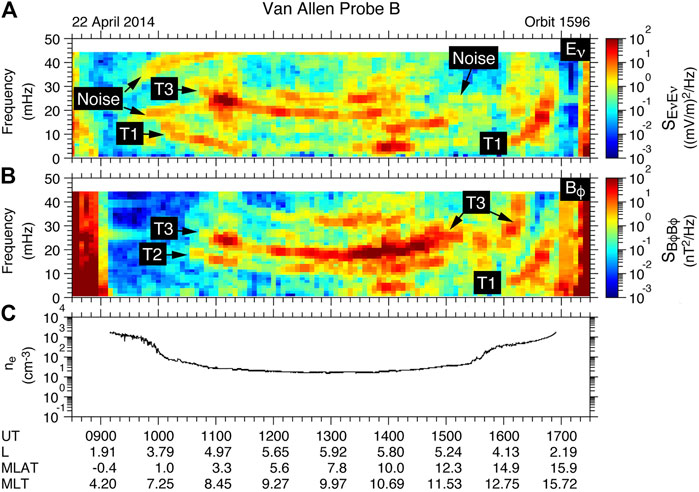
FIGURE 1. Time-frequency dynamic spectrograms of electric and magnetic field power measured by Van Allen Probe B on 22 April 2014. (A) Spectral power $S_{E_{\nu }{E}_{\nu }}$ of the radial component of the electric field, E_ν; (B) spectral power $S_{B_{\varphi }{B}_{\varphi }}$ of the azimuthal component of the magnetic field, B_ϕ; and (C) the electron density inferred from plasma wave data. The fundamental mode, second harmonic, and third harmonic are labeled “T1,” “T2,” and “T3,” respectively [Adapted from Figure 5 of Takahashi and Denton (2021).].

In Section 2 we discuss the data used in this study, in Section 3 we discuss our methods, and in Section 4 we discuss our results. Discussion and conclusion follow in Section 5.

2 Data

2.1 Alfvén frequencies

When wave field power is plotted in a “dynamic spectrogram,” with time on the horizontal axis, and frequency on the vertical axis, the wave power often is concentrated in harmonic bands. These bands correspond to global eigenmodes of magnetospheric field lines (e.g., Figure 1 of Takahashi and Denton, 2021). Fast mode waves propagating through the magnetosphere with a particular frequency will preferentially be converted to Alfvén waves with the same eigenmode frequency (Chen and Hasegawa, 1974).

Although eigenmodes can occur with magnetic field and velocity perturbations in either the azimuthal or radial direction, for the purposes of measuring the mass density, frequencies of azimuthally oscillating magnetic field and velocity are preferable because magnetic oscillations in the radial direction tend to be compressional, with frequencies depending on the plasma pressure gradient (Denton, 1998). Thus for this study, we confine ourselves to oscillations predominantly in the azimuthal direction, the so-called “toroidal” mode (oscillating around the torus of magnetospheric plasma).

Figure 1 shows example dynamic spectrograms for the field data measured by Van Allen Probe B. The fields were expressed in terms of field aligned coordinates with azimuthal (ϕ) and radial (ν) components perpendicular to the background magnetic field. The toroidal mode has radial electric field and azimuthal wave magnetic field, so both Figures 1A,B show toroidal mode power. Toroidal harmonics occur with antinodes at different locations for the electric and magnetic field, so the different wave power versus magnetic latitude, MLAT, and the phase between these fields can be used to identify the harmonics unambiguously (Takahashi and Denton, 2021). The fundamental mode, second harmonic, and third harmonic in Figure 1 are labeled “T1”, “T2”, and “T3”, respectively.

Ordinarily, the frequency of a particular harmonic will decrease as the spacecraft moves outward. The frequency of the T3 mode in Figure 1B has a minimum at maximum L shell near 1300 UT. But as the spacecraft moves inward (lower L) after 1300 UT, the frequency of the T3 mode drops near 1535 UT because the plasmapause was crossed at that time, as shown in Figure 1C. Roughly, the frequency of the Alfvén wave is proportional to $V_A/L\propto {\rho }_m^{-0.5}$, where $V_A\equiv B/\sqrt{{\mu }_0{\rho }_m}$ is the Alfvén speed, B is the magnitude of the background magnetic field, and μ₀ is the vacuum permeability. So when the spacecraft crosses into the high density plasmasphere at 1535 UT, the frequency of the Alfvén wave decreases. Aside from the increase in density at that time, the Alfvén frequency would increase since the magnetic field increases as the spacecraft moves inward toward the earth.

2.2 Database

We created two databases, a larger one with the mass density observations, and a smaller one with simultaneous mass and electron density observations. Our modeling proceeded through many iterations in which we examined the dependence of ρ_m and M on many different parameters: position; phase of the year; geomagnetic indices like Kp, Dst, and AE; solar wind parameters like components of the interplanetary magnetic field (IMF), B_Y and B_Z, the solar wind density, solar wind velocity, V, and solar wind dynamic pressure, Pdyn; the F10.7 index measuring solar radiation at 10.7 cm wavelength; the solar wind convection electric field defined by VB_s, where B_s = −B_Z if B_Z < 0 and B_s = 0 otherwise; and the coupling function of Newell et al. (2007), dΦ_MP/dt. For those parameters that had a significant influence on ρ_m or M, we considered various averages or extrema, for instance the average or extremum within the last 3, 6, 12, 24, … 192 h. For instance, one of the terms in some of our models for M is AE_12h, where the subscript “12h” indicates a boxcar average of AE over the previous 12 h. F10.7 varies slowly, and appeared unaveraged in some models. But some models showed a preference for F10.7_3day, which is an average of F10.7 with an exponentially falling weight with a 3 days timescale; i.e.,

${\mathrm{F}\mathrm{10.7}}_{3\text{\hspace{0.17em}day}}=\frac{{\int }_{t_1}^t\mathrm{F}\mathrm{10.7}\text{exp}\left(-\left(t-t^{\prime }\right)/\left(3\text{days}\right)\right)d{t}^{\prime }}{{\int }_{t_1}^t\text{exp}\left(-\left(t-t^{\prime }\right)/\left(3\text{days}\right)\right)d{t}^{\prime }}(1)$

evaluated at time t with the lower limit of integration t₁ ≪ t. There is a similar term with a 3 days average of Kp. Unaveraged Kp appeared in just one model.

We limited our data to 1.3 ≤ L ≤ 10. We screened the observations of M to require that for AE_12hr the “quality factor” (as defined by Qin et al. (2007)) was at least 1, meaning that the 12 h average of AE was mostly calculated from times where or near to where AE was measured. Averages of Pdyn appeared in some models of both ρ_m and M. We did not screen the quality factors for these averages because the Kondrashov et al. (2014) database of solar wind parameters that we used in early years, when measurements of Pdyn were not always available, did a good job of modeling Pdyn. (See Section 3 for more information.).

We also screened observations of M to require 0.5 ≤ M ≤ 23. A physically reasonable range is 1 (for all H+) to 16 (for all O+). Many of our observations show a peak centered at M = 1 with a width partially related to the uncertainty in the measurements. We allow values less than 1 as input to the models so as not to bias the models. Considering that we allowed a factor of two lower M values than M = 1, one might consider using M = 32 as an upper limit for observations. But there are very few observations with M approaching 16. The use of 23 as an upper limit was a logarithmic compromise between 16 and 32. Only 2.5% of our M values were rejected because they fell outside of the range between 0.5 and 23.

For application of the models, however, we limit the range of M to between 1 and 16. That is, M values less than 1 are changed to 1, and values of M greater than 16 are changed to 16. This adjustment was made for both observations and model results when calculating the statistical error of the models.

2.3 Missions

Observations of Alfvén frequencies by the GOES were determined from magnetic field oscillations, as described by Takahashi et al. (2010). Because all of these measurements were at geostationary orbit, and because we had so many Alfvén frequencies from GOES compared to those from other spacecraft, we cut the data down by a factor of three from nearly 500,000 frequencies to 165,272. The measurements were made between 1980 and 1992, a complete solar cycle. The number of frequencies measured by each mission, N_unweighted, used for developing models for both ρ_m and M is listed in Table 1. For GOES, n_e was not measured, so no values are listed for M. The weighted number of observations, N_weighted, is also listed in Table 1. Weighting of the data will be described in Section 2.4.

TABLE 1

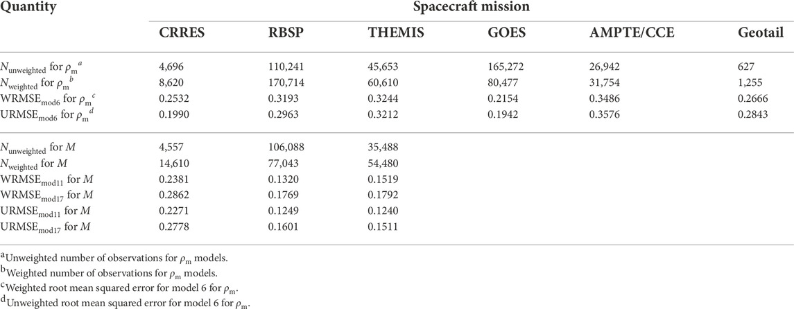
TABLE 1. Spacecraft Mission number of observations and model errors.

AMPTE/CCE had an Apogee of 8.8 R_E. Alfvén frequencies detected by the AMPTE/CCE magnetometer between 1984 and 1989 were described by Min et al. (2013). This time period was centered on a solar minimum, but contained data in declining and rising stages of the solar cycle. In this case, only the third harmonic frequencies were used. There were 26,942 measurements.

The CRRES spacecraft had an elliptical orbit with apogee near geostationary orbit. Alfvén frequencies observed by CRRES were determined from oscillations of the electric field, as described by Takahashi et al. (2006). Based on the linearized magnetohydrodynamic (MHD) equation, dE = −dV × B₀, azimuthal velocity perturbations correspond to radial (or “poloidal”) electric field perturbations. There were 4,696 frequencies observed by CRRES occurring during 1990 and 1991, at solar maximum. The first half of that time period was relatively geomagnetically quiet as determined by the Kp index, but the second half was extremely active.

For CRRES, electron density measurements are also available that made use of the Plasma Wave Experiment (PWE) on CRRES (LeDocq et al., 1994). The electron density was found either from the upper hybrid frequency band or from the lower edge of continuum radiation for electromagnetic waves propagating within the plasmatrough. Electron density measurements were available for 4,557 of the 4696 CRRES mass density measurements.

Fundamental Alfvén wave frequencies (T1) were identified for the Geotail spacecraft using the bulk velocity from Geotail’s low energy particle experiment (Takahashi et al., 2014, and references therein). These were obtained between 1995 and 2006, a complete solar cycle, but there were only 627 measurements after screening the data for L and agreement between the model and observed magnetic field (see Section 3.3). These were all between L = 9 and 10, since the spacecraft perigee was about 9 R_E.

THEMIS frequencies were determined from magnetometer data using the same technique that Min et al. (2013) used to analyze data from the AMPTE/CCE and GOES spacecraft. We made use of data from the THEMIS A, D, and E spacecraft, with apogees of about 10 R_E, 12 R_E, and 12 R_E respectively. There were 45,653 frequencies observed at solar minimum between 2007 and 2011. Frequencies for one harmonic were manually identified for each orbit. Other harmonics were identified based on their frequency ratio relative to the identified harmonic. These occurred in most cases in well-defined peaks that could be differentiated. When frequencies were not in well differentiated peaks, they were discarded. The electron density at the THEMIS spacecraft location was inferred from the spacecraft potential using the technique of Nishimura et al. (2013); 35,488 of the 45,653 mass density measurements also had electron density data.

The two Van Allen Probes, or RBSP (Radiation Belts Storm Probes), spacecraft had an apogee of about 6 R_E. Alfvén frequencies were determined from electric and magnetic field data using the techniques described by Takahashi and Denton (2021). There were 110,241 frequencies observed between 2012 and 2014. This time period was during the early part of a very weak solar maximum. There were electron density measurements from plasma wave data (Kurth et al., 2015) for 106,088 of the 110,241 mass density measurements.

2.4 Weighting

Because of the uneven distribution of frequencies for various conditions, we used variable weights with values between 1 and 30. Preliminary weights for our ρ_m measurements were set equal to the product of w_L, w_F10.7, and w_MLT. These were defined in the following way. The number of events was counted in 17 bins of L between L = 1.5 and 10, 12 bins of F10.7 between 50 and 350 solar flux units, (sfu, or 10^–22 W s/m²), and 24 bins of MLT covering the entire range between 0 and 24 h. These three quantities were found to be the most important in the models. For each quantity, a weight was defined for each bin equal to the maximum number of observations in any bin divided by the number of observations in the particular bin. For instance, if the maximum number of observations in any bin of L were 10,000, and another bin of L had 1,000 observations, the weight for that other bin would be 10,000/1,000 = 10. For a particular observation at L, the log of the binned weights was interpolated to that L value, and then w_L was the anti-log of the interpolated value. This procedure would lead to weights greater than or equal to unity, but if the product w_Lw_F10.7w_MLT was greater than 30, it was set to 30. Finally, after all the weights were defined, they were divided by the average weight, so that the average of the final weights was unity.

If the weights were defined with only one factor, like w_L, there might be many observations with weights differing by a factor of 30. But because of the product of three different weights, most data points had a weight greater than unity before normalization of the distribution. We find $10^{{\sigma }_w}=2.5$ where σ_w is the standard deviation of the base 10 logarithm of the weights, suggesting that about two-thirds of the data had weights falling within 1/2.5 = 0.4 and 2.5.

The weights for the observations of M were defined similarly, except that w_Kp3day was substituted for w_MLT, where w_Kp3day was defined in a similar fashion using 8 bins of Kp_3day between 0 and 8.

The resulting distribution of observations is shown versus year of observation, L, solar EUV F10.7 index, Kp_3day, MLT, and n_e in Figure 2. Note that Figure 2, like most of our other figures, makes use of two part panel labels; here uppercase letters indicate the panel row, and lowercase letters indicate the panel column. The unweighted distributions are shown as blue curves, while the weighted distributions are shown as red curves. The majority of data points (blue curves in Figure 2) occur near geostationary orbit at L = 6.6, at F10.7 less than 150 sfu, at Kp_3day less than 2, and on the dayside between MLT = 5 and 15. Weighting the distributions of data points for ρ_m results in a flatter and broader distribution of data points with respect to L, F10.7, and MLT (comparing the red curves to the blue curves in Figures 2Ba,Ca,Ea). For M, the weighted distribution is more evenly distributed for Kp_3day rather than for MLT (comparing the red curves to the blue curves in Figures 2Db, Eb). This makes sense considering that the weighting of ρ_m data points used the distribution of MLT, whereas the weighting of M used the distribution of Kp_3day, as described above. It should be kept in mind that the ranges of data with the most observations mentioned above will most strongly influence the models. Nevertheless there are significant numbers of data points for a much broader range of conditions. For instance, L values between 3 and 10 are well represented.

FIGURE 2

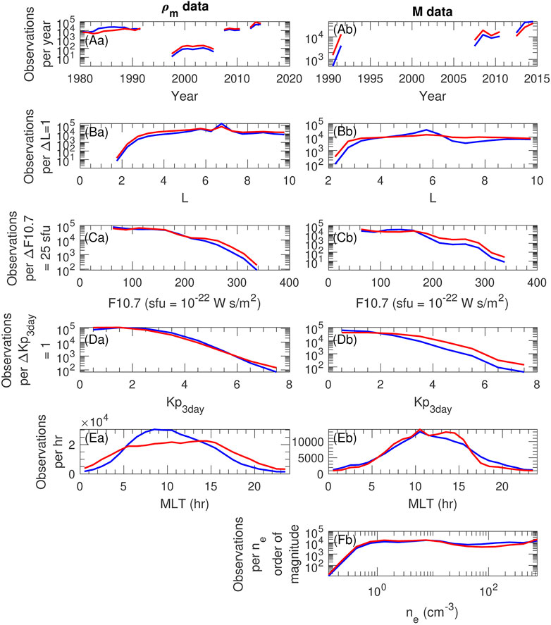
FIGURE 2. Unweighted (blue curves) and weighted (red curves) distribution of observations for (a) ρ_m and (b) M. Distributions versus (A) year, (B) L, (C) solar EUV F10.7 index, (D) Kp_3day, (E) MLT, and (F) n_e. Except for the MLT distributions in (E), the vertical axes are logarithmic.

The distribution of M values in our database is shown in Figure 3. Figures 3A–C show histograms for the individual missions, with a linear scale on the vertical axis in the left column, and a logarithmic scale in the right column. The weighted distribution for all the data is shown in Figures 3D. There is a significant number of events with 0.5 < M < 1, but as discussed previously, this is to be expected because of the large number of observations with M close to unity (pure H+ plasma) and the uncertainties of the data. In all cases, even for THEMIS (Figure 3Ca), the number of observations steeply decreases for M values below 1. And the agreement between mass density and electron density in Figure 3 is considerably better than the agreement between the electron density determined from plasma wave measurements on the Dynamics Explore 1 (DE-1) mission and the total ion density measured by the DE-1 Retarding Ion Mass Spectrometer (RIMS) particle instrument that has been used in studies of ion composition (Craven et al., 1997; Goldstein et al., 2019) (not shown).

FIGURE 3

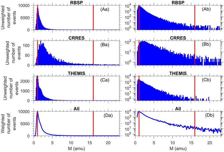
FIGURE 3. Distributions of M values in bins of width 0.1. Histograms of the unweighted number of events of M values for the (A) Van Allen Probes (RBSP), (B) CRRES, (C) THEMIS, and (D) the weighted distribution of the combined data set, plotted with a (a) linear or (b) logarithmic vertical axis. The red vertical lines are at M = 1 and M = 16, the limits of realistic M values for a plasma consisting of H+, He+, and O+.

2.5 Test data

One tenth of the data was separated off for testing the models. This data was not used as input to the models. The procedure for separating the data was as follows. The data files were first sorted by time. Then they were divided into segments based on time. Within each segment, the inner 10th of data was selected as test data. Three hundred segments were used for the ρ_m data file, and fifty segments were used for the smaller M data file (smaller because only CRRES, RBSP, and THEMIS had n_e data). By having a large number of data segments and segments of test data within the segments of input data, we ensure that the long-term sampling of conditions is similar, while the precise conditions and locations were different. The average time interval of the test data for the ρ_m data was 3.3 days, and that for the M data was 3.5 days. Our intent was to make this time interval large enough so the data in the test segments would have locations and geomagnetic indices uncorrelated with that of the data used for the model. A better method would be to have a buffer between the two types of data. But our method of separation is clearly better than a random selection, for which data points in the set used for developing the model are temporarily adjacent to data points used for test data. That type of separation essentially leads to the same data in the two sets.

3 Methods

3.1 Solution for ρ_m

To solve for the mass density, we used the Singer et al. (1981) wave equation with an azimuthal perturbation at the magnetic equator. A perfect conducting ionospheric boundary was assumed at an altitude of 100 km. The Singer et al. equation requires a magnetic field model; we used the TS05 model (Tsyganenko and Sitnov, 2005) with inputs from the Kondrashov et al. (2014) solar wind parameter database supplemented by the Qin et al. (2007) database for time periods not included in the Kondrashov et al. (2014) database.

Our set of observations includes different Alfvén wave harmonics, which except for THEMIS (as described in Section 2.3), were identified using techniques described by Takahashi and Denton (2021).

3.2 Field line dependence

All mass densities shown in this paper are equatorial values. In order to solve for the mass density, we need to assume a distribution of mass along magnetic field lines. We use the commonly used power law form,

${\rho }_{\text{m,MLAT}}={\rho }_{\text{m,eq}}{\left(\frac{L}{R}\right)}^{\alpha },(2)$

where ρ_m,MLAT is the magnetic latitude (MLAT) dependent mass density, and ρ_m,eq is the equatorial mass density, defined to be the value at largest geocentric radius R_max = LR_E, where R_E is the radius of the Earth. While we used the symbol ρ_m,eq here for clarity, to distinguish it from ρ_m,MLAT, elsewhere ρ_m will also refer to the equatorial mass density.

Motivated by results discussed by Denton (2006), we use for α at L ≤ 4.5,

${\alpha }_1\equiv 11.25-3.05L+0.225L^2.(3)$

This form allows for greater mass loading at very low L values, i.e., larger α leading to larger ρ_m at small R.

Based on results by Denton et al. (2015), who modeled the field line dependence at geostationary orbit, we use for α at L ≥ 6.6,

$\begin{array}{ll}\hfill {\alpha }_2& =2.2+1.3\text{cos}\left(2\pi \mathrm{M}\mathrm{L}\mathrm{T}/24\right)+0.0026\mathrm{A}\mathrm{E}\cdot \text{cos}\left(2\pi \left(\mathrm{M}\mathrm{L}\mathrm{T}-0.8\right)/24\right)\hfill \\ \hfill & +2.1\times 10^{-5}\mathrm{A}\mathrm{E}\cdot \mathrm{F}\mathrm{10.7}-0.010\mathrm{F}\mathrm{10.7}.\hfill \end{array}(4)$

Between L = 4.5 and 6.6, we define f₂ ≡ (L − 4.5)/1.1 and f₁ ≡ 1 − f₂, and use α = f₁α₁ + f₂α₂.

However, any calculated values of α greater than 4 are set equal to 4, and any calculated values of α less than -4 are set equal to -4.

Despite the effort put into modeling the field line dependence, the effect of different α values on the equatorial mass density is small. Testing the CRRES data set using the above combination of α₁ and α₂ versus just using a nominal value of α = 1, yielded a standard deviation in the base 10 logarithm of only 0.03, corresponding to an 8% difference in results.

For calculating M, we used Eq. 2 to solve for ρ_m,MLAT at the spacecraft location, and then divided that value by the electron density at the spacecraft location to get M. We made a mistake, however, when creating the database used as input to the models. Although we used the mass density at the spacecraft location for the Van Allen Probes data, we used the mass density at the equator for CRRES and THEMIS data. We regenerated models using a corrected database, but the difference in the models was not great enough to redo all the results in the paper. This is not totally surprising considering that CRRES and especially THEMIS had low inclination orbits, so there should not be a big difference between the mass density at the equator and that at the spacecraft location using Eq. 2. All plots in the paper use the corrected data, and the model errors in Table 2 were calculated using the corrected data. Only the exact form of the models described in Table 2 was influenced by the non-corrected data.

TABLE 2

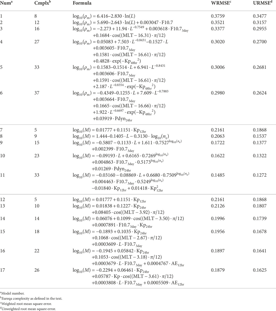
TABLE 2. Models.

3.3 Uncertainties

For data points at large L, particularly for L > 8, there may be significant error in the calculation of ρ_m due to the inaccuracy of the magnetic field model. In order to mitigate this last problem, we calculated the error parameter dB = |B_obs − B_TS05|/|B_obs| for the three missions with the largest orbit apogees, AMPTE/CCE, CRRES, and THEMIS, and rejected all observations with dB > 0.2.

The largest uncertainty for many ρ_m data points is likely to be the uncertainty in the observed frequencies. We have determined frequency uncertainties for some of the missions. Median values of df/f for Alfvén frequencies measured by CRRES, Geotail, and the Van Allen Probes are 12%, 10%, and 11%, where f is the frequency and df is its uncertainty converted from full width at half maximum to a standard deviation for a Gaussian shape. Taking 11% as a typical value, and considering that the mass density is inversely proportional to the square of the frequency (Section 2.1), there would be a typical uncertainty in the mass density of 22%.

The uncertainty for electron density based on measurements of the plasma frequency from the Van Allen Probes is at least 10% based on the frequency resolution, and usually no more than 20% (Hartley et al., 2016). The uncertainty for electron density based on the plasma frequency measured by CRRES was estimated to be accurate to 12% by Carpenter et al. (2000). The uncertainty of the THEMIS electron density determined from the spacecraft potential is difficult to evaluate, but the typical error for events examined by Nishimura et al. (2013) is about 20%–30%.

Figure 3Da also suggests that the uncertainty of most of our data points is small. Taking the left side of the peak at M = 1, the half width at half maximum is at M = 0.69, suggesting that the standard deviation of M might be as low as 0.26 (26% of 1), and that estimate is for the combined errors of mass density and electron density.

3.4 Generation of models using Eureqa

Finally, once databases were created for ρ_m and M, the Eureqa nonlinear genetic regression program (Schmidt and Lipson, 2009), a proprietary product owned by the DataRobot company, was used to generate formulas for ρ_m and M. Eureqa searches the space of formulas, adding terms and operations to seek the best formula for each level of complexity. In our case, the complexity of a newly introduced variable or constant was 1, that of a simple mathematical operation like a sum, difference or product was 1, that for raising to a power was 1, and that for functions like a logarithm or exponential was 3. MLT values were introduced using a cosine function with a phase so as to ensure continuity around the Earth. For each level of complexity, the model with the least error is chosen. We used for the error the weighted root mean standard deviation between the observed and model values.

4 Results

4.1 One dimensional dependence

Figure 4 shows one dimensional distributions of ρ_m or M in evenly spaced bins of parameters that occurred in some of the models. Figure 4A shows that ρ_m decreases with increasing L, decreases slightly and then increases with respect to increasing Kp, and increases with increasing F10.7. There is a peak in ρ_m in the dusk local time sector between 15 < MLT $<21$.

FIGURE 4

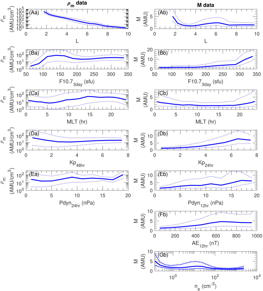
FIGURE 4. One dimensional distributions of (a) ρ_m and (b) M versus parameters used in some of the models. The solid curve is the log averaged value of ρ_m or M in evenly spaced bins of (A) L, (B) F10.7_3day, (C) MLT, (D) Kp_48hr for ρ_m or Kp_24hr for M, (E) Pdyn_24hr for ρ_m or Pdyn_12hr for M, and (F) AE_12hr and (G) n_e for M only. The dotted curves show the log average plus or minus the logarithmically calculated standard deviation.

Figure 4B shows that M increases with increasing F10.7, Kp, Pdyn, and AE, and decreases with increasing n_e. M is larger at very low L and there is a small local peak in M near L = 6. There is also a peak in M close to midnight (MLT = 0 or 24).

Because some of the parameters are interrelated, particularly the geomagnetic activity indices, all of the specific dependencies observed in Figure 4 may not appear in the models. Even some of the spatial dependencies might be prejudiced if there was a greater likelihood of certain activity levels at certain locations. As we will show in Section 4.6, such an effect does occur and accounts for the local peak in M in Figure 4Ab.

4.2 Models

Using Eureqa, we selected seven models for the base 10 logarithm of ρ_m, seven models for the base 10 logarithm of M using the spacecraft n_e values as input, and seven models for the base 10 logarithm of M not using n_e as input. Formulas making use of n_e would be valuable for spacecraft that provide routine measurement of n_e. The formulas could also be combined with a model for n_e to get ρ_m throughout the magnetosphere.

We model the logarithm of ρ_m because of the huge range of its variation. Logarithmic values of M were used because M is calculated as a ratio of two numbers. Another advantage of using logarithms is that the model values of ρ_m and M are necessarily positive.

In Table 2, the model number is in the first column, the Eureqa complexity level is in the second column, the mathematical formula is in the third column, the weighted root mean squared error of the model (WRMSE) is in the fourth column, and the unweighted root mean squared error (URMSE) is in the fifth column. The values for WRMSE and URMSE in Table 2 are the larger of the error calculated using the input data and the error calculated using the test data. The standard deviation is calculated in the usual way, but its use does not imply that the distributions of errors are exactly Gaussian. For instance, the distribution of log₁₀ (M_mod17) − log  10₁₀(M_obs), where M_mod17 is the value from model 17 and M_obs is an observed value, has a slightly negative skew (broader tail for negative values).

Although increasing complexity in the models always resulted in lower WRMSE for the data used as input to the model, in some cases increased complexity did not result in lower standard error for the test data. We rejected models if by allowing additional complexity any error (weighted or unweighted using input or test data) did not decrease with respect to additional complexity. We ended up with six models for ρ_m (models 1–6), five models for M using the spacecraft n_e values as input (models 7–11), and six models for M not using n_e as input (models 12–17).

4.3 Model errors

It might seem strange that the unweighted errors in Table 2 (URMSE) are smaller than the weighted errors (WRMSE), because the models were chosen in order to minimize WRMSE, not URMSE. The reason why the URMSE values are smaller is probably that the weighting emphasizes extreme conditions for which it is difficult to accurately model the dependencies. (The differences in values using input or test data were smaller than the differences from using weighted or unweighted errors.)

Taking the URMSE values as more representative of most data points, and recognizing that we are modeling the logarithmic values, we can find a multiplicative error for the non-logarithmic quantity by taking 10^URMSE. For instance, if URMSE for log₁₀ (ρ_m) were unity, most of the model values for ρ_m would be within a factor of 10 lower and a factor of 10 higher than the observed values. The most complex model listed for log₁₀ (ρ_m), model 6, has URMSE = 0.2581, indicating that ρ_m can be determined from the model within a factor of 10^0.2581 = 1.81. The most complex model listed for log₁₀(M) using n_e values as input, model 11, has URMSE = 0.1272, indicating that M can be determined within a factor of 1.34. The most complex model listed for log₁₀(M) not using n_e values as input, model 17, has URMSE = 0.1625, indicating that M can be determined within a factor of 1.45 if n_e is not known.

Figure 5 shows observed and modeled values of ρ_m (Figure 5a) and M (Figure 5b) for RBSP-A during 24 days of 2013. Sometimes the model values are higher than the observed values, and sometimes they are lower, but the models capture many of the trends in the observations. The red dots in Figure 5b are from model 11 using n_e as input to the model, whereas the pink curves in Figure 5b are from model 17 that does not use n_e as an input to the model. At most times, the results from these two models are similar, but model 11 appears to represent the observed values slightly better at some times (e.g., day of 2013 at 148.6, near 152.8, at 153.4, 154.9, 155.8, 156.1, 156.9, and 158.3, near 159 and 161, and at 167.3, 169.9, and 171.8).

FIGURE 5

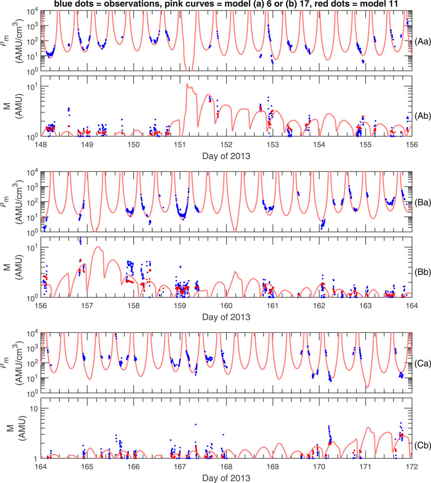
FIGURE 5. Observed and modeled values of (a) ρ_m and (b) M for RBSP-A during 24 days of 2013 divided into three groups, (A), (B), and (C). The blue dots are the observed values. The pink curves are model values, (a) model 6 for ρ_m, and (b) model 17 for M; both of these depend only on the spacecraft position and activity indices. The red dots in (b) are model values using model 11, which uses values of n_e.

Table 2 shows that use of more complicated models yields diminishing returns as the complexity of the model is increased. For instance, going from model 1 to model 2, URMSE decreases by 0.032. But going from model 5 to model 6, URMSE decreases by only 0.01.

For the most common complicated models, models 6, 11, and 17, errors for data from individual missions are listed in Table 1. As expected, the errors listed in Table 2 for those models are within the range of values for individual missions. The smallest errors for ρ_m using model 6 occur for the spacecraft that sample only the smallest L values, CRRES and GOES. Somewhat surprisingly, then, the largest errors for M occur for CRRES. Since M is calculated from ρ_m and n_e, presumably then the greater error in M for CRRES is because of greater uncertainty in n_e; this could well be because CRRES sampled the most active conditions for which the plasmapause position and electron density are more uncertain.

4.4 Model dependencies

As the models in Table 2 increase in complexity, one can see which parameters are most important for determining the modeled quantities. For instance, when modeling ρ_m, the strongest dependence is on L, as suggested by model 1. The second strongest dependence is on F10.7, as suggested by model 2. The third strongest dependence is on MLT, as suggested by model 3. Model 4 introduces a dependence on Kp, in addition to refining the dependence on L. Model 5 introduces a term depending on both L and Kp, and model 6 introduces a dependence on Pdyn.

Ranking the importance of the parameters for modeling M is somewhat more complicated. Model 7 (or equivalently, model 12, which is the same since neither of these models includes n_e dependence) suggests that if only one parameter is included in the model, it should be an average of Kp. But model 8 shows that a more accurate model can be achieved by dropping the Kp dependence and including dependence on L and n_e together. The fact that all the subsequent models 9–11 include dependence on both L and n_e, and that Kp dependence is only reintroduced in the most complicated model, model 11, suggests that the most important dependence is on L and n_e together. Model 9 adds F10.7 dependence, model 10 adds Pdyn dependence, and model 11 drops the Pdyn dependence but adds a more complicated dependence on F10.7 and Kp.

Model 13, modeling M without n_e dependence, adds MLT dependence to the Kp dependence of model 12. Model 14 drops the linear Kp dependence but adds a product of Kp and F10.7. Model 15 keeps linear Kp dependence and adds a product of L and F10.7. Model 16 adds AE dependence and model 17 has an MLT-dependent term multiplied by Kp.

4.5 Residual model dependencies

Figure 6 is like Figure 4 except that the observed values ρ_m,obs at each data point have been divided by ρ_m,mod using model 6, and model values M_mod have been subtracted from the observed values M_obs using model 11 (with the observed n_e as an input parameter) or model 17 (without n_e as an input parameter). If the model were perfectly removing the average dependencies shown in Figure 6, the solid blue curves would be exactly along the horizontal dotted gray lines at ρ_m,obs/ρ_m,mod = 1 and M_obs −M_mod = 0. Smaller separation of the dotted blue curves from ρ_m,obs/ρ_m,mod = 1 and M_obs −M_mod = 0 indicates smaller standard deviation between the observed and model results.

FIGURE 6

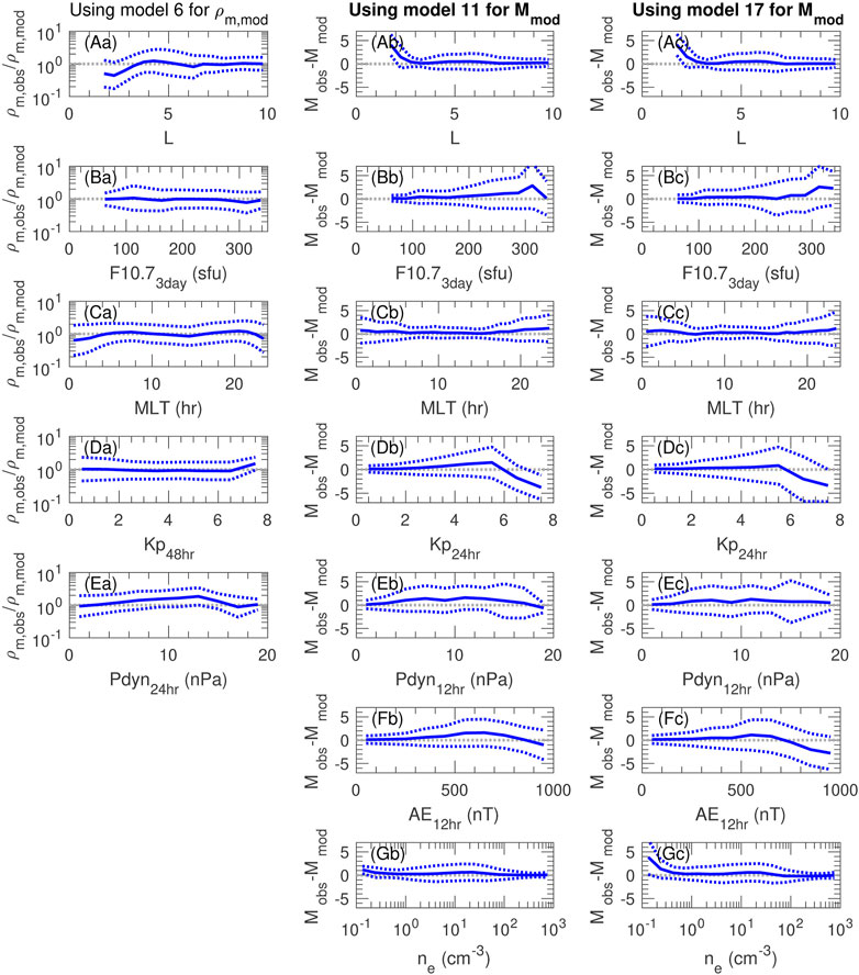
FIGURE 6. One dimensional residual distributions of (a) ρ_m and (b,c) M versus parameters used in some of the models. This plot shows the same quantities in rows (A–G) as were shown in Figure 4 except that the observed values ρ_m,obs at each data point have been divided by ρ_m,mod using model 6, and model values M_mod have been subtracted from the observed values M_obs using (b) model 11 (with the observed n_e as an input parameter), and (c) model 17 (without n_e as an input parameter).

Figure 6a shows that model 6 removes most of the average dependence of ρ_m,obs on the variables plotted. There is some residual error for L < 3.5, MLT near midnight, and values of Pdyn_24hr > 7 nPa.

Figures 6b,c show that models 11 and 17, respectively, remove most of the average dependence of M_obs on the variables plotted. There is some residual error for L < 3, F10.7_3day > 300 sfu, Kp_24hr > 6, and AE_12hr > 500 nT, and for n_e < 0.3 cm⁻³ when using model 17 (Figure 6c).

The conditions for which the average residual is large are those for which there are fewer data points. For instance, Figure 2 shows that there are relatively fewer observations for small L, large F10.7, large Kp_3day, and small n_e.

4.6 Distributions in the equatorial plane

Figure 7 shows distributions of ρ_m (Figures 7A,B) and M (Figures 7C,D) in the equatorial plane. Plots using all available data are shown for ρ_m in Figures 7A and for M in Figures 7C. Since ρ_m increases with respect to F10.7 (Figure 4Ba and model 2 in Table 2) and M increases with respect to Kp (Figure 4Db and model 7 or 12 in table 2), we show stronger driving for ρ_m by limiting the data to F10.7_3day > 220 sfu in Figures 7B and for M by limiting the data to Kp_3day > 2.5 in Figures 7D.

FIGURE 7

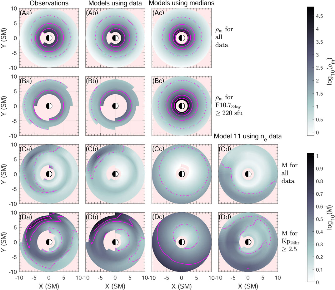
FIGURE 7. Two dimensional distributions of the average (A,B) ρ_m and (C,D) M in SM (Solar Magnetic, or dipole) coordinates in the equatorial plane. Rows A and C use all available data, while row B (for ρ_m) requires F10.7_3day > 220 sfu, and row D (for M) requires Kp_3day > 2.5. In column (a) we show the binned distributions of the observations; in column (b) we show binned distributions of model values using model 6 for ρ_m and model 17 (not depending on n_e) for M and using input geomagnetic activity parameters at the times of the observations; in column (c) we show distributions using the same models, but using median geomagnetic activity parameters for the data sets shown; and in column (d) we show distributions for M using model 11 with binned observed values of n_e, but using median geomagnetic activity parameters for the data sets shown. Pink areas are either outside 2 ≤ L ≤ 10 or have fewer than 5 observations in a bin. In (A–B), the dotted magenta contours are at ρ_m = 10 amu/cm³ and the broken or solid contours at values of 100, 1,000, and 10⁴ amu/cm³. In (C–D), the dotted magenta contours are at M = 2, and the broken or dotted contours are at M = 4 and 6 (The dotted curve at the upper left of panel Db is spurious.) Please note that the distributions in columns (a), (b), and (d) are not characteristic of all conditions.

Figures 7A, using all the data, show that ρ_m decreases steeply with respect to L, with little MLT dependence other than a slight bulge toward dusk local time (at the top of the plots). Comparing the distributions for ρ_m using all the data (Figures 7A) to those with higher F10.7_3day (Figures 7B), we see that larger F10.7_3day leads to larger ρ_m as expected. Average binned values of ρ_m using model 6 evaluated with input of geomagnetic activity parameters at the times of the observations (Figures 7Ab,Bb) or with input of median geomagnetic activity parameters for the data sets shown (Figures 7Ac,Bc) yield similar results to binned averages of the observed ρ_m values (Figures 7Aa,Ba). There are small differences, like a broader distribution of M ≤ 2 in Figures 7Ba,Bb compared to Figure 7Bc, but the differences in Figures 7C,D are much greater, and we will now focus our attention on explaining those.

Values of M in Figures 7D, for which the data has been limited to Kp_3day > 2.5, are significantly larger than those in Figures 7C, for which all available data has been used, matching our expectations. But there are significant differences between the spatial distributions of M depending on how they are calculated. The dependence that we expect based on model 17 in Table 2 is that shown in Figures 7Cc,Dc, where M increases with larger L and at MLT = 3.61 (dawn local time at the lower left of the plots).

If the distribution of geomagnetic activity values were well sampled at a particular spatial location, then the average model values of M at that location using the geomagnetic activity values at the times of observations should be similar to those calculated with median geomagnetic activity values. The fact that the distributions in Figures 7Cb,Db, showing binned averages of model 17 evaluated with input of geomagnetic activity parameters at the times of the observations, are significantly different from those in Figures 7Cc,Dc, showing the spatial distribution from model 17 using median geomagnetic activity parameters, suggests that the geomagnetic conditions in different spatial regions are not the same.

The binned averages of model 17 evaluated with input of geomagnetic activity parameters at the times of the observations (Figures 7Cb,Db) are fairly similar to the binned averages of the observed M values in Figures 7Ca,7Da, suggesting that the particular geomagnetic activity levels in different spatial regions explains the observed values. Using n_e in model 11 with median geomagnetic activity parameters (Figures 7Cd,Dd) does not lead to significantly better agreement with the observed values (Figures 7Ca,7Da), again suggesting that it is different sampling of geomagnetic activity in different spatial regions that is causing the difference between observed results and the model results using median geomagnetic activity values.

In order to understand how the spatial distributions in Figures 7Da,Db depend on the different sampling of geomagnetic activity in different spatial regions, we plot in Figure 8 spatially binned values of quantities needed to evaluate M using model 17 for two cuts through the equatorial plane. The data in Figure 8 are limited to Kp_3day > 2.5 as was used for Figures 7D. There are two major differences between the distribution of M in Figures 7Da,Db and that in Figure 7Dc. The first is the different MLT dependence. At large L, Figure 7Dc shows M peaking at dawn local time (lower left portion of the plot), whereas Figure 7Da shows M peaking at pre-midnight local time (upper left portion of the plot).

FIGURE 8

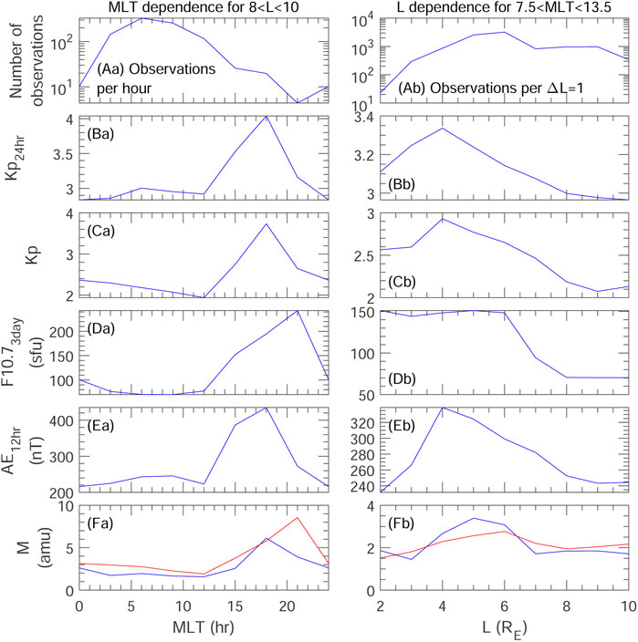
FIGURE 8. For Kp_3day > 2.5, spatially binned values of quantities needed to evaluate model 17 for M, versus (a) MLT limiting the data to 8 < L < 10, and (b) L limiting the data to 7.5$<$MLT$<$13.5. The blue curves show (A) the number of (unweighted) observations per (a) hr or (b) ΔL = 1, and average binned values of (B) Kp_24hr, (C) Kp, (D) F10.7_3day, (E) AE_12hr, and (F) M. In row (F), the red curves show the value of M from model 17 (not depending on n_e) using the average binned geomagnetic activity parameters in rows (B–E). Please note that the distributions of M here are not characteristic of all conditions.

Figure 8a shows for 8 < L < 10 the MLT dependence of the number of observations, the average geomagnetic activity values, and M (blue curves). Along with the average M values in Figure 8Fa (blue curve), the red curve shows the values of model 17 for M using the averaged binned geomagnetic activity levels for input. The values of model 17 based on the geomagnetic activity levels (red curve in Figure 8Fa) are quite similar to the values based on the observations (blue curve), apparently because of the peaks in Kp, F10.7, and AE in the pre-midnight local time sector (18 h $<$ MLT $<$ 24 h), which are quite prominent in Figures 8Ba–8Ea. Note that the number of observations is relatively small at this location (Figure 8Aa), which could more easily lead to unusual values of geomagnetic activity there.

The second major difference between the distribution of M in Figures 7Da,7Db and that in Figure 7Dc is the L dependence. Figure 7Da appears to show that there is a local peak in M at about L = 5. This feature is most clear in the late morning local time sector. Figure 8b shows the same data as in Figure 8a, except that here it shows the L dependence limiting the data to 7.5$<$MLT$<$13.5. Again, the red curve in Figure 8Fb, showing model 17, is quite similar to the blue curve, both having a peak at L = 5; this agreement shows that the different geomagnetic activity conditions sampled at different L account for the distribution of the observed M values. Model 17 in Table 2 has terms proportional to Kp, AE, and one proportional to the product of L and F10.7_3day. Values of Kp and AE in Figures 8Bb, 8Cb, 8Eb increase up to L = 4 and then decrease for larger L. The model M value (red curve in Figure 8Fb) continues to increase to L = 6 because of the term proportional to L F10.7_3day, but then decreases for larger L due to the precipitous drop in F10.7_3day at L = 6 (Figure 8Db). This is because in the database for M, only THEMIS sampled large L, and the THEMIS measurements were at solar minimum with low F10.7.

5 Discussion

Using the mass density calculated from toroidal (azimuthally oscillating) frequencies of magnetospheric Alfvén waves measured by six different spacecraft missions, and using the mass density along with electron density calculated from plasma wave or spacecraft potential data for three of those missions, we generated models for the mass density ρ_m and average ion mass M. By using the nonlinear genetic regression algorithm Eureqa (Schmidt and Lipson, 2009), we were able to find analytical formulas that can be easily interpreted. For both ρ_m and M, we found families of models of varying complexity, which are listed in Table 2.

5.1 Dependencies in model 6 for ρ_m

By looking at which parameters occur in the whole range of models, we can determine which parameters are most important. The terms in model 6 are arranged in roughly the order of most importance. The most important parameter for modeling ρ_m seems to be L, followed by the EUV solar radiation index F10.7, followed by MLT, followed by the geomagnetic activity index Kp, followed by the solar wind dynamic pressure Pdyn. Other than the positions, these quantities most often appear in the models as averages over time, as described in Section 2.2.

Most of the dependencies in model 6 can be easily understood. Because magnetospheric H+ primarily comes from the ionosphere, plasmaspheric density decreases with respect to L. Larger F10.7 increases the scale height of oxygen in the ionosphere, which in conjunction with other processes gets more O+ into the magnetosphere (Takahashi et al., 2010; Denton et al., 2011). Because of the convection pattern around the Earth, the plasmasphere bulges out on the duskside and the flow may stagnate there (Denton et al., 2014b). Even outside of the plasmasphere, the density is higher on the dusk side (Denton et al., 2006). The Kp index correlates strongly with magnetospheric convection. Larger Kp means that density is swept out of the magnetosphere in the plasmatrough which is outside the plasmasphere. The term $1.922\cdot L^{-0.6697}\cdot \text{exp}(-{{\mathrm{K}\mathrm{p}}_{48\text{hr}}}^2)$ in model 6 decreases with increasing Kp. Although the strength of this term decreases with increasing L, the rate of decrease is less than that due to the pure L dependence. Therefore relative to the density apart from this term, the dependence is stronger at larger L. One dependence we did not understand is that on Pdyn.

5.2 Dependencies in model 11 for M

Similarly, the terms in model 11, which models M using n_e as an input parameter, are arranged in an approximate order of importance. The most important parameters are L and n_e together, followed by F10.7, followed by Kp (although Kp is the first parameter to show up in the simplest model, as discussed in Section 4.4).

At first glance, the L-dependent term would seem to imply that M uniformly decreases with respect to L. However, the $0.6680\cdot 0.7509^{{\text{log}}_{10}(n_{\text{e}})}$ term in model 11 decreases with respect to log₁₀ (n_e) (as does the simpler −0.3130 log₁₀ (n_e) term in model 8), and log₁₀ (n_e) decreases with respect to L. Therefore these two terms have opposite L dependencies. Model 17 without n_e dependence suggests that the combination of the two terms results in an increase in M with respect to L.

As suggested by the discussion in Section 5.2, greater F10.7 is expected to lead to more O+, which would increase M. The $0.004463{\mathrm{F}\mathrm{10.7}}_{3\text{day}}\cdot 0.5249^{{\text{log}}_{10}(n_{\text{e}})}$ term in model 11 shows that this effect is greater for smaller log₁₀ (n_e), that is, in the plasmatrough.

Next consider the Kp dependence in model 11. For Kp_12hr < 0.6, M increases with decreasing Kp, but for Kp_12hr > 0.6, M increases with respect to increasing Kp. The stronger factor is the increase at large Kp suggested also by Figure 4Db. Larger Kp sweeps away the plasma, but may also lead to increased outflow of O+.

Although there is no explicit MLT dependence in model 11, n_e will be largest in the afternoon local time sector, where the plasmasphere tends to bulge outwards; so the $0.6680\cdot 0.7509^{{\text{log}}_{10}(n_{\text{e}})}$ term will lead to decreased M there where there is a greater percentage of H+ relative to O+ (more “plasmasphere-like” plasma).

5.3 Dependencies in model 17 for M

Model 17 is a formula for M without using log₁₀ (n_e) as an input parameter. In model 17, the Kp dependence seems to be strongest, followed by MLT, then F10.7, and finally AE.

Model 17 has M increasing with respect to Kp as already discussed in Section 5.2. The MLT dependence shows a peak in M at dawn (MLT = 3.61) where the H+ density is low and the plasma is more “plasmatrough-like.” The MLT-dependent term is multiplied by Kp, showing that this dawn peak in M is most pronounced with larger activity. (This is the only term in any of the models that used a non-averaged value of Kp.) More solar radiation as specified by F10.7 leads to larger M at larger values of L, similar to the dependence on F10.7 described in Section 5.2. Finally larger AE leads to larger M, probably because the greater activity leads to more O+ outflow.

5.4 Conclusion

Using the Eureqa nonlinear genetic regression algorithm (Schmidt and Lipson, 2009) we developed analytical models, listed in Table 2, by using a database of mass density and electron density values from six spacecraft missions. In Table 2, models one to six are for the magnetospheric equatorial mass density, ρ_m; models 7–11 are for the average ion mass, M, if n_e is available for input; and models 12–17 are for M if n_e is not available for input. Models are listed with varying complexity; one can choose a simpler or more complex model depending on the need. More complex models are more accurate, but the incremental increase in accuracy with respect to complexity becomes less for greater complexity. Chaotic properties might make it difficult or impossible to model the density much more accurately by including more information as input to the models. The most complex models appearing in this paper are capable of modeling ρ_m within a factor of 1.81, and M within a factor of 1.34 if n_e is used as an input parameter, or within a factor of 1.45 if n_e is not used as an input parameter.

It may be possible to get some increase in accuracy by modeling ρ_m and M using other machine learning techniques, such as neural networks, support vector regression, or time history methods. But our analytical models are useful for understanding the processes that lead to greater ρ_m and M. We have provided explanations for most of the dependencies in these formulas.

By using a multivariate analysis, we were able to tease out the spatial dependence of ρ_m and M separated from the influence of geomagnetic activity (shown in Figure 7c). If, however, we had used only the traditional technique of spatial binning in Figure 7a, we would have concluded that the spatial dependence of these quantities is quite different. This demonstrates the danger of finding spatial distributions when the conditions sampled are different in different regions. In our case, different spacecraft data were collected at different times in different regions of space; and the activity conditions were not the same during the different times of the missions. But this problem could also occur for a single mission. For example, CRRES sampled the morning local time sector when the geomagnetic activity as indicated by Kp was typically very low, but it sampled the afternoon local time sector when the geomagnetic activity was often much larger.

Our results differ somewhat from those of Lee and Angelopoulos (2014). The concentrations of heavy ions in their Figures 7C, 8C would imply that M is larger than our values at large L with a peak in M in the pre-midnight local time sector. Our models also did not infer the radially localized “oxygen torus” discussed by Nose et al. (2018) (and references therein). Our models have increasing M with respect to L. But Nose et al. (2018) event was observed during storm time, while we were examining all conditions. We did find that M is peaked longitudinally at MLT = 3.6 near the dawn location inferred by Nose et al. (2018).

Our data should be separated into the plasmasphere and plasmatrough data to learn more.

Data availability statement

The observed Alfvén frequencies and inferred mass density values used in this manuscript are in a Zenodo repository at https://doi.org/10.5281/zenodo.7098025. Also included is a file with input parameters for the TS05 magnetic field model (Tsyganenko and Sitnov, 2005). The geomagnetic activity indices used to create that input file are available at the NASA Goddard “OMNIWeb Plus’’ website, https://omniweb.gsfc.nasa.gov. GOES data are available at https://www.ngdc.noaa.gov/stp/satellite/goes/dataaccess.html. AMPTE/CCE data are available at http://sd-www.jhuapl.edu/AMPTE/MAG/SA_Data/. CRRES data, including electron density based on plasma wave measurements, are available at http://vmo.igpp.ucla.edu/data1/CRRES/. Van Allen Probes data, including electron density based on plasma wave measurements, are available at the NASA Goddard “CDAWeb” website, https://cdaweb.gsfc.nasa.gov. Geotail and THEMIS magnetometer data are also available at CDAWeb. THEMIS electron density based on spacecraft potential is available through the Space Physics Environment Data Analysis Software (SPEDAS, at https://spedas.org/blog) using the Interactive Data Language (IDL) program “thm\_scpot\_density.pro''. Eureqa can be run online at a website provided by the DataRobot company (https://www.datarobot.com/); after a free trial period, computer time on their system can be purchased from DataRobot for a nominal fee. The data in the Zenodo repository (see the Data Availability Statement) are described in the Supplementary Material README document that is in the repository.

Author contributions

RD did all of the modeling and wrote the paper. All other authors read the manuscript and provided feedback to RD. KT calculated Alfvén wave frequencies for most of the spacecraft missions. KM calculated the Alfvén frequencies for AMPTE/CCE and THEMIS. DH represents the University of Iowa group that provided electron densities for the CRRES and RBSP missions. YN provided help for obtaining the electron density from the spacecraft potential measured by the THEMIS spacecraft.

Funding

RD and KT were supported by NASA grants 80NSSC20K1446 and 80NSSC21K0453. KM was supported by the National Research Foundation of South Korea (NRF) grant funded by the South Korea government (MSIT), 2020R1C1C1009996. YN was supported by NASA grant 80NSSC21K1321 and NSF grant AGS-1907698.

Acknowledgments

We thank Dennis Gallagher for useful conversations about ion measurements by the Retarding Ion Mass Spectrometer (RIMS) that was on the Dynamics Explorer 1 (DE-1) spacecraft.

Conflict of interest

The authors declare that the research was conducted in the absence of any commercial or financial relationships that could be construed as a potential conflict of interest.

Publisher’s note

All claims expressed in this article are solely those of the authors and do not necessarily represent those of their affiliated organizations, or those of the publisher, the editors and the reviewers. Any product that may be evaluated in this article, or claim that may be made by its manufacturer, is not guaranteed or endorsed by the publisher.

References

Andre, M. (1985). Dispersion Surfaces. J. Plasma Phys. 33, 1–19. doi:10.1017/s0022377800002270

CrossRef Full Text | Google Scholar

Carpenter, D. L., Anderson, R. R., Calvert, W., and Moldwin, M. B. (2000). CRRES observations of density cavities inside the plasmasphere. J. Geophys. Res. 105, 23323–23338. doi:10.1029/2000ja000013

CrossRef Full Text | Google Scholar

Chappell, C. R. (1988). The Terrestrial Plasma Source - A New Perspective In Solar-Terrestrial Processes From Dynamics Explorer. Rev. Geophys. 26, 229–248. doi:10.1029/RG026i002p00229

CrossRef Full Text | Google Scholar

Chen, L., and Hasegawa, A. (1974). plasma-heating by parametric-instabilities excited near lower hybrid frequencies. Bulletin of the American Physical Society 19, 882–882.

Google Scholar

Craven, P. D., Gallagher, D. L., and Comfort, R. H. (1997). Relative concentration of He+ in the inner magnetosphere as observed by the DE 1 retarding ion mass spectrometer. J. Geophys. Res. 102, 2279–2289. doi:10.1029/96ja02176

CrossRef Full Text | Google Scholar

Denton, R. E. (1998). Compressibility of the poloidal mode. J. Geophys. Res. 103, 4755–4759. doi:10.1029/97ja02652

CrossRef Full Text | Google Scholar

Denton, R. E. (2006). “Magneto-seismology using spacecraft observations,” in Magnetospheric ULF waves: Synthesis and new directions. Editors K. Takahashi, P. J. Chi, R. E. Denton, and R. L. Lysak (Washington, DC: American Geophysical Union).

CrossRef Full Text | Google Scholar

Denton, M. H., Borovsky, J. E., Skoug, R. M., Thomsen, M. F., Lavraud, B., Henderson, M. G., et al. (2006). Geomagnetic storms driven by ICME- and CIR-dominated solar wind. J. Geophys. Res. 111, A07S07. doi:10.1029/2005JA011436

CrossRef Full Text | Google Scholar

Denton, R. E., Thomsen, M. F., Takahashi, K., Anderson, R. R., and Singer, H. J. (2011). Solar cycle dependence of bulk ion composition at geosynchronous orbit. J. Geophys. Res. 116. doi:10.1029/2010ja016027

CrossRef Full Text | Google Scholar

Denton, R. E., Jordanova, V. K., and Fraser, B. J. (2014a). Effect of spatial density variation and O+ concentration on the growth and evolution of electromagnetic ion cyclotron waves. JGR. Space Physics 119, 8372–8395. doi:10.1002/2014ja020384

CrossRef Full Text | Google Scholar

Denton, R. E., Takahashi, K., Thomsen, M. F., Borovsky, J. E., Singer, H. J., Wang, Y., et al. (2014b). Evolution of mass density and O+ concentration at geostationary orbit during storm and quiet events. JGR. Space Physics 119, 6417–6431. doi:10.1002/2014ja019888

CrossRef Full Text | Google Scholar

Denton, R. E., Takahashi, K., Lee, J., Zeitler, C. K., Wimer, N. T., Litscher, L. E., et al. (2015). Field line distribution of mass density at geostationary orbit. JGR. Space Physics 120, 4409–4422. doi:10.1002/2014ja020810

CrossRef Full Text | Google Scholar

Denton, R. E., Takahashi, K., Amoh, J., and Singer, H. J. (2016). Mass density at geostationary orbit and apparent mass refilling. JGR. Space Physics 121, 2962–2975. doi:10.1002/2015JA022167

CrossRef Full Text | Google Scholar

Goldstein, J., Gallagher, D., Craven, P. D., Comfort, R. H., Genestreti, K. J., Mouikis, C., et al. (2019). Temperature dependence of plasmaspheric ion composition. J. Geophys. Res. Space Physics 124, 6585–6595. doi:10.1029/2019JA026822

CrossRef Full Text | Google Scholar

Hartley, D. P., Kletzing, C. A., Kurth, W. S., Bounds, S. R., Averkamp, T. F., Hospodarsky, G. B., et al. (2016). Using the cold plasma dispersion relation and whistler mode waves to quantify the antenna sheath impedance of the Van Allen Probes EFW instrument. J. Geophys. Res. Space Physics 121, 4590–4606. doi:10.1002/2016JA022501

CrossRef Full Text | Google Scholar

Kondrashov, D., Denton, R., Shprits, Y. Y., and Singer, H. J. (2014). Reconstruction of gaps in the past history of solar wind parameters. Geophys. Res. Lett. 41, 2702–2707. doi:10.1002/2014gl059741

CrossRef Full Text | Google Scholar

Krall, J., Huba, J. D., and Fedder, J. A. (2008). Simulation of field-aligned H+ and He+ dynamics during late-stage plasmasphere refilling. Ann. Geophys. 26, 1507–1516. doi:10.5194/angeo-26-1507-2008

CrossRef Full Text | Google Scholar

Kress, B. T., Hudson, M. K., Looper, M. D., Albert, J., Lyon, J. G., and Goodrich, C. C. (2007). Global MHD test particle simulations of >10 MeV radiation belt electrons during storm sudden commencement. J. Geophys. Res, 1. doi:10.1029/2006ja012218

CrossRef Full Text | Google Scholar

Kurth, W. S., De Pascuale, S., Faden, J. B., Kletzing, C. A., Hospodarsky, G. B., Thaller, S., et al. (2015). Electron densities inferred from plasma wave spectra obtained by the Waves instrument on Van Allen Probes. JGR. Space Physics 120, 904–914. doi:10.1002/2014JA020857

PubMed Abstract | CrossRef Full Text | Google Scholar

LeDocq, M. J., Gurnett, D. A., and Anderson, R. R. (1994). Electron number density-fluctuations near the plasmapause observed by the CRRES spacecraft. J. Geophys. Res. 99, 23661–23671. doi:10.1029/94ja02294

CrossRef Full Text | Google Scholar

Lee, J. H., and Angelopoulos, V. (2014). On the presence and properties of cold ions near Earth’s equatorial magnetosphere. J. Geophys. Res. Space Physics 119, 1749–1770. doi:10.1002/2013ja019305

CrossRef Full Text | Google Scholar

Menk, F. W. (2011). “Magnetospheric ULF waves: A review,” in Dynamic magnetosphere. Editors W. Lui, and M. Fujimoto. doi:10.1007/978-94-007-0501-2_13

CrossRef Full Text | Google Scholar

Min, K., Bortnik, J., Denton, R. E., Takahashi, K., Lee, J., and Singer, H. J. (2013). Quiet time equatorial mass density distribution derived from AMPTE/CCE and GOES using the magnetoseismology technique. J. Geophys. Res. Space Physics 118, 6090–6105. doi:10.1002/jgra.50563

CrossRef Full Text | Google Scholar

Min, K., Liu, K. J., Wang, X. Y., Chen, L. J., and Denton, R. E. (2018). Fast Magnetosonic Waves Observed by Van Allen Probes: Testing Local Wave Excitation Mechanism. JGR. Space Physics 123, 497–512. doi:10.1002/2017ja024867

CrossRef Full Text | Google Scholar

Newell, P. T., Sotirelis, T., Liou, K., Meng, C. I., and Rich, F. J. (2007). A nearly universal solar wind-magnetosphere coupling function inferred from 10 magnetospheric state variables. J. Geophys. Res. 112. doi:10.1029/2006ja012015

CrossRef Full Text | Google Scholar

Nishimura, Y., Bortnik, J., Li, W., Thorne, R. M., Ni, B., Lyons, L. R., et al. (2013). Structures of dayside whistler-mode waves deduced from conjugate diffuse aurora. JGR. Space Physics 118, 664–673. doi:10.1029/2012JA018242

CrossRef Full Text | Google Scholar

Nose, M., Matsuoka, A., Kumamoto, A., Kasahara, Y., Goldstein, J., Teramoto, M., et al. (2018). Longitudinal structure of oxygen torus in the inner magnetosphere: Simultaneous observations by arase and van allen probe A. Geophysical Research Letters 45, 10177–10184. doi:10.1029/2018GL080122

CrossRef Full Text | Google Scholar

Nose, M., Oimatsu, S., Keika, K., Kletzing, C. A., Kurth, W. S., De Pascuale, S., et al. (2015). Formation of the oxygen torus in the inner magnetosphere: Van Allen Probes observations. JGR. Space Physics 120, 1182–1196. doi:10.1002/2014ja020593

CrossRef Full Text | Google Scholar

Olsen, R. C., Chappell, C. R., Gallagher, D. L., Green, J. L., and Gurnett, D. A. (1985). the hidden ion population - revisited. J. Geophys. Res. 90, 12121–2132. doi:10.1029/ja090ia12p12121

CrossRef Full Text | Google Scholar

Qin, Z., Denton, R. E., Tsyganenko, N. A., and Wolf, S. (2007). Solar wind parameters for magnetospheric magnetic field modeling. Space Weather 5. doi:10.1029/2006SW000296

CrossRef Full Text | Google Scholar

Sandhu, J. K., Yeoman, T. K., Fear, R. C., and Dandouras, I. (2016). A statistical study of magnetospheric ion composition along the geomagnetic field using the Cluster spacecraft for L values between 5.9 and 9.5. J. Geophys. Res. Space Physics 121, 2194–2208. doi:10.1002/2015JA022261

CrossRef Full Text | Google Scholar

Schmidt, M., and Lipson, H. (2009). Distilling Free-Form Natural Laws from Experimental Data. Science 324, 81–85. doi:10.1126/science.1165893

PubMed Abstract | CrossRef Full Text | Google Scholar

Singer, H. J., Southwood, D. J., Walker, R. J., and Kivelson, M. G. (1981). Alfven-Wave Resonances in a Realistic Magnetospheric Magnetic-Field Geometry. J. Geophys. Res. 86, 4589–4596. doi:10.1029/ja086ia06p04589

CrossRef Full Text | Google Scholar

Takahashi, K., and Denton, R. E. (2021). Magnetospheric mass density as determined by ULF wave analysis. Front. Astron. Space Sci. 8. Tex.orcid-numbers: Takahashi, Kazue/0000-0003-1434-4456 tex.researcherid-numbers: Takahashi, Kazue/H-3060-2016 Denton, Richard/AGE-4634-2022 tex.unique-id: WOS:000697400600001. doi:10.3389/fspas.2021.708940

CrossRef Full Text | Google Scholar

Takahashi, K., Denton, R. E., Anderson, R. R., and Hughes, W. J. (2006). Mass density inferred from toroidal wave frequencies and its comparison to electron density. J. Geophys. Res. 111, A01201. doi:10.1029/2005JA011286

CrossRef Full Text | Google Scholar

Takahashi, K., Denton, R. E., Hirahara, M., Min, K., Ohtani, S.-i., and Sanchez, E. (2014). Solar cycle variation of plasma mass density in the outer magnetosphere: Magnetoseismic analysis of toroidal standing Alfven waves detected by Geotail. J. Geophys. Res. Space Physics 119, 8338–8356. doi:10.1002/2014ja020274

CrossRef Full Text | Google Scholar

Takahashi, K., Denton, R. E., and Singer, H. J. (2010). Solar cycle variation of geosynchronous plasma mass density derived from the frequency of standing Alfven waves. J. Geophys. Res. 115. doi:10.1029/2009ja015243

CrossRef Full Text | Google Scholar

Takahashi, K., Ohtani, S., Denton, R. E., Hughes, W. J., and Anderson, R. R. (2008). Ion composition in the plasma trough and plasma plume derived from a Combined Release and Radiation Effects Satellite magnetoseismic study. J. Geophys. Res. 113. doi:10.1029/2008JA013248

CrossRef Full Text | Google Scholar

Tsyganenko, N. A., and Sitnov, M. I. (2005). Modeling the dynamics of the inner magnetosphere during strong geomagnetic storms. J. Geophys. Res. 110, A03208. doi:10.1029/2004ja010798

CrossRef Full Text | Google Scholar