The need for accurate measurements of thermal velocity distribution functions in the solar wind

1 Introduction

The solar wind is a weakly collisional ionized gas experiencing collective effects due to long-range electromagnetic forces. Unlike a collisionally mediated fluid like Earth’s atmosphere, the solar wind is not in thermodynamic or thermal equilibrium. That is, the particles are not in equipartition of energy (i.e., different species have different temperatures) and there is nearly always a finite heat flux present in the solar wind plasma near 1 AU [e.g., (Wilson et al., 2018; Wilson et al., 2019a; Wilson et al., 2019b; Wilson et al., 2020)].

Weakly collisional in this context refers to the large separation between Coulomb collisional mean free paths and relevant spatial scales like thermal gyroradii, ρ_cs, and/or inertial lengths, λ_s. The collisional mean free path of thermal particles near Earth are on the order of one astronomical unit or 1 AU ∼ 1.5 × 10⁸ km (Wilson et al., 2018; Wilson et al., 2019b). The typical thermal proton gyroradius and inertial length near Earth satisfy 30 km ≲ ρ_cp ≲ 190 km and 50 km ≲ λ_p ≲ 130 km [e.g., (Wilson et al., 2021)], i.e., nearly six orders of magnitude smaller than the collisional mean free path. It is therefore surprising that particle-particle collisional signatures are actually observed in the particle velocity distribution functions (VDFs) [e.g., (Salem et al., 2003; Maruca et al., 2013)]. Yet there are just as many studies showing evidence of VDF modification due to turbulence and/or instabilities¹ [e.g., (Maruca et al., 2012; Kasper et al., 2013; Wilson et al., 2020)].

The fundamental issue is that research is often limited to fluid velocity moments of a VDF and rarely do we have full 3D VDFs available. If we do, the VDFs are often of limited resolution or counting statistics. The solar wind ion VDFs are of particular interest but are the least well resolved of all VDFs that instruments have measured to date. The ions can dominate in momentum and energy transport² and often control the dynamics of fundamental plasma phenomena, but we are still greatly limited in our ability to resolve the core solar wind because it is such a fast and cold beam. We are also greatly limited in our observations of electron VDFs in the solar wind. Note that higher order velocity moments like the heat flux tensor require high resolution (i.e., energy and angle) measurements to properly calculate. The electron heat flux is very difficult to properly calculate but the ion species-dependent heat fluxes are even more problematic with low resolution or crude methods [e.g., see discussion by (Scudder, 2015)].

While the detailed shape/profile of any given VDF may seem to be a nuanced issue, it is well known that instabilities can be very sensitive to deviations in the VDF away from a Maxwellian, for instance [e.g., (Goldman et al., 2007; Lazar et al., 2012; Lazar et al., 2013; Lazar et al., 2014; Lazar et al., 2017; Lazar et al., 2018; Shaaban et al., 2018; Lazar et al., 2019; Lee et al., 2019; Shaaban et al., 2019)]. Even if we ignore non-Maxwellian features, the presence of multiple Maxwellians will alter instability thresholds and our interpretation of the corresponding velocity moments [e.g., (Chen et al., 2016; Husidic et al., 2020; Verniero et al., 2020; Klein et al., 2021)]. If we cannot resolve a VDF with sufficient accuracy to elucidate these features, we will both find an apparent lack of correspondence between observations and theory. Further, under resolved VDFs preclude our ability to properly document even the macroscopic energy inputs into critical systems like collisionless shock waves (Schwartz et al., 2022). Therefore, it is of fundamental importance for all aspects of plasma physics that we properly resolve the VDFs in any given region of space being examined.

The following is an expanded discussion of the White Paper by (Wilson et al., 2022) submitted to the Decadal Survey for Solar and Space Physics (Heliophysics) 2024–2033. The paper is outlined as follows: Section 3 describes our current understanding; Section 4 describes some current and future measurements for reference; Section 5 illustrates why high resolution measurements are necessary by comparing to MMS observations; Section 6 discusses what needs to be done to properly resolve solar wind distributions; Section 7 illustrates how low resolution and/or incomplete measurements can result in very inaccurate velocity moments; and Section 8 summarizes our discussion and conclusions.

2 What is known

In the solar wind near Earth, the electrons are comprised of four primary populations: a cold dense core with energies typically below ∼15 eV; a hot, tenuous halo with energies from several 10s of eV to ∼1–2 keV; an anti-sunward, field-aligned beam called the strahl with energies from a few 10s of eV up to ∼1–2 keV; and a higher energy superhalo with energies ≳1 keV [e.g., (Wilson et al., 2019a; Wilson et al., 2019b; Wilson et al., 2020), and references therein]. In contrast, the ion VDF is comprised of dozens of mass per charge species but the primary constituents are a cold dense proton core, a differentially drifting proton beam, and a differentially drifting alpha-particle beam [e.g., (Alterman et al., 2018), and references therein].

Traditionally, the core electrons have been modeled as a bi-Maxwellian, the halo and/or strahl as bi-kappas, and the superhalo as a power-law VDF [e.g., (Wang et al., 2012; Wilson et al., 2019a), and references therein]. However, recent analysis of electron VDFs near collisionless shocks have revealed that the core electron population is better modeled by what is called a self-similar distribution (Wilson et al., 2019a; Wilson et al., 2019b; Wilson et al., 2020). These functions can be used to model the so called “flattop” or “flat-top” electron VDF. Recent Parker Solar Probe measurements have shown that even the core proton population can exhibit a flattop profile (Martinović et al., 2020). These observations suggest the proton core shares the same multitude of populations as the electrons below ∼1 keV in the solar wind.

What’s perhaps more confusing is how to reconcile the implications for the self-similar distribution, given that the deviation from a bi-Maxwellian is evidence of inelastic collisions (Wilkinson and Edwards, 1982; Martin and Piasecki, 1999; Alvarez Laguna et al., 2022). This realization was made when comparing to studies of flow through disordered porous media and shocks in coarse grain media (Villani, 2006; Siena et al., 2014; Matyka et al., 2016).

3 What is unknown

The solutions to the Vlasov equation (i.e., collisionless Boltzmann equation) are, by construction, time-reversible functions. Similarly, the solutions to the original Boltzmann equation are time-irreversible functions. The standard Boltzmann collision operator assumes two-particle elastic collisions and molecular chaos³, among other things. It is through this latter assumption that the entire operator can generate a time-irreversible result (Bhatnagar et al., 1954; Gressman and Strain, 2010). These two equations are commonly used to model the evolution of plasmas in simulations.

The surprising aspect of the recent electron observations was the realization that the deviation from Maxwellian to a self-similar VDF is a quantified measure of inelastic collisions [e.g., see discussions in (Wilson et al., 2019a; Wilson et al., 2019b; Wilson et al., 2020)]. Inelastic collisions are intrinsically a time-irreversible process. Self-similar distributions were predicted in quasi-linear and nonlinear theory of wave-particle interactions decades ago [e.g., (Vedenov, 1963; Sagdeev, 1966; Dum et al., 1974; Dum, 1975)]. An analogous operator to that generating inelastic collisions can arise indirectly through approximations like coarse grain averaging, but what is lost through such averaging? While the connection to a fundamentally irreversible phenomena remains unknown, it does seem possible for irreversible processes to arise in plasmas [e.g., (Villani, 2014)].

Thus, the realization that the particle VDFs in the solar wind can exhibit signatures of inelastic collisions is of fundamental importance to kinetic theory, space plasma physics, and astrophysics. The question is, how do inelastic collisions occur? Further, if such inelastic processes are important near collisionless shocks, are they important everywhere in the solar wind? Are these irreversible processes unknowingly hidden in our estimates of collisionality? What is more important for the evolution of VDFs, collisional effects or waves/turbulence?

Further, our inability to properly resolve the thermal ion populations precludes our ability to address outstanding questions like the partition of energy amongst the constituent particle populations in any fundamental plasma phenomena. This is especially problematic for collisionless shock waves. If we cannot properly account for the ion populations incident on the shock, we have no proper baseline for the most important input to the system, i.e., the upstream ion kinetic energy density. Further, if our measurements effectively “smear out” the ion VDF, we cannot discriminate whether the ion VDF changes shape across the shock or how it evolves. This leaves us with crude parameters like the total ion temperature, which can be extremely misleading in such kinetic processes [e.g., (Wilson et al., 2014a; Wilson et al., 2014b; Goldman et al., 2020; Wilson et al., 2020; Goldman et al., 2021; Argall et al., 2022)].

4 Current and planned measurements

The primary current thermal plasma instruments making measurements in the solar wind near Earth are from Wind 3DP and SWE (Wilson et al., 2021), THEMIS electrostatic analyzers or ESAs (McFadden et al., 2008a; McFadden et al., 2008b), and MMS FPI (Pollock et al., 2016). The THEMIS and MMS instruments were designed to measure the hot, slow magnetospheric and magnetosheath plasmas. Thus, they tend to over estimate the temperature and underestimate the number density of particles in the solar wind [e.g., (Wilson et al., 2014a; Artemyev et al., 2018; Roberts et al., 2021)]. The PESA Low instrument from Wind/3DP measures ions with an angular resolution of $\sim 5.6°$ and an energy resolution of ∼20%. The EESA Low instrument from Wind/3DP measures electrons with an angular resolution of $\sim 11.25°$ and an energy resolution of ∼20%. The SWE Faraday cups measure ions with an energy resolution of ∼6.5–13% and angular resolution of $\sim 8°$. The best time cadence of both of the 3DP ESAs ∼3 s whereas the SWE Faraday cups are at ∼92 s [e.g., see (Wilson et al., 2021), and references therein].

Newer thermal particle instruments on Parker Solar Probe (PSP) (Kasper et al., 2016) and Solar Orbiter (SolO) (Nicolaou et al., 2019) have made improvements with angular resolutions of $\sim 5°$–6° for SolO and $\sim 5°$–11.25° for PSP. Instrumentation on both spacecraft have energy resolutions of ∼7%. The nominal time resolutions⁴ are ∼3.5 and ∼4 s, respectively. Since both PSP and SolO are significantly closer to the Sun than Wind, the typical time scales of interest (e.g., cyclotron period) are much shorter. Thus, the increased time resolution on SolO compared to, say, Wind, is not as advantageous as it would be were the spacecraft located near Earth. The future IMAP mission (McComas et al., 2018) will have both thermal electron and ion particle measurements. The electron instrument will have an angular resolution of ≳ 12° and an energy resolution of ∼12% at a cadence of ∼15 s. The ion instrument will have an energy resolution of ∼8.5% at a cadence of ∼15 s and is meant for measuring bulk solar wind properties. Therefore, the IMAP instruments make some improvements in energy resolution over Wind, but the time resolution is five times lower.

In short, there are no current or future planned instrumentation that will properly resolve the thermal solar wind plasma populations.

5 Comparison with MMS

The purpose of this section is to help illustrate that what can appear to be a minor nuance (i.e., changes or deviations in a VDF or low counting statistics or under resolved peaks) actually becomes a major problem in some regions of space. Although the MMS FPI instrument is unparalleled in the magnetosheath and magnetosphere, it was not designed for the cold, fast solar wind. There are a great deal of extra efforts “behind the scenes” by the FPI team to improve and validate the data products in these regions, which can sometimes hide the issue at hand or give false confidence to an unknowing researcher. Below we outline why a great deal of caution is necessary when using FPI data in the solar wind and why MMS cannot address the issue of solar wind measurements.

Both the DES and DIS detectors (Pollock et al., 2016), part of the fast plasma investigation (FPI) on MMS, systematically over estimate the temperature, T_s,tot, and under estimate the number density, n_s, in the solar wind [e.g., (Roberts et al., 2021)]. The reason being that the energy and angular resolution of the detectors were designed for a slow-moving, hot plasma. The solar wind, by comparison to the magnetosphere, is a fast-moving, very cold plasma. Further, under most bow shock crossings, the MMS FPI instrument is not in its solar wind mode thus the minimum energy bin, E_min, is above the spacecraft potential, ϕ_SC. This means the instrument is missing part or most of the solar wind core electrons, depending on conditions. Further, due to the often large number of secondary and photoelectrons (Gershman et al., 2017), the signal-to-noise ratio (SNR) of any given DES energy-angle bin in the solar wind can be quite small.

Figure 1 shows an illustrative comparison between a Wind 3DP EESA Low (Wilson et al., 2021) and MMS DES (Pollock et al., 2016) electron VDF. In both cases, the data are corrected for ϕ_SC and transformed into the bulk flow rest frame following the procedures discussed in the appendices of Wilson III et al. (Wilson et al., 2019a). The MMS DES VDF had the secondary and photoelectrons removed (Gershman et al., 2017), following the procedures outlined in the SPEDAS software (Angelopoulos et al., 2019). The Wind 3DP VDF was chosen roughly 1 hour earlier than the DES VDF to correspond to the propagation time of the solar wind. The SNR shown here is illustrated by the ratio between the 1D cuts (i.e., red or blue lines in the bottom panels) to that of the Poisson statistics (i.e., magenta lines). One can see that DES only has a few energy-angle bins with sufficient count rates⁵ to be statistically significant. In contrast, all energy-angle bins have sufficient count rates for the Wind 3DP VDF.

FIGURE 1

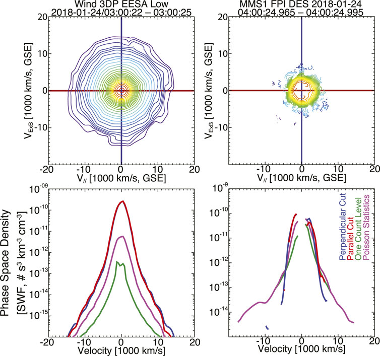
FIGURE 1. Illustrative example electron VDFs from Wind 3DP (Wilson et al., 2021) and MMS DES (Pollock et al., 2016). The top row shows contours of constant phase space density [cm⁻³ km⁻³ s⁺³] of a two-dimensional cut through a three-dimensional VDF. The plane and coordinate basis are defined by the quasi-static magnetic field, B_o, and the ion bulk flow velocity, V_i. The vertical axis is defined by the unit vector $\left({\mathbf{B}}_o\times {\mathbf{V}}_i\right)\times {\mathbf{B}}_o$ and the horizontal by B_o. The bottom row shows one-dimensional cuts of the VDF along the horizontal (solid red line) and along the vertical (solid blue line). The location of these cuts are defined by the color-coded cross hairs in the top row panels. Also shown are the one-count (solid green line) and Poisson statistics (solid magenta line) levels for reference. The VDF is shown in the ion bulk flow rest frame.

This should not be surprising as 3DP was designed for the solar wind and accumulates for a full spacecraft spin period (∼3 s) whereas DES was not designed for the solar wind and only accumulates for ∼0.03 s (i.e., ∼100 times shorter duration). Note that the FPI team does some extra work to help “fill in” the gap at low energies and help correct the electron velocity moments to account for these issues (e.g., several personal communications with FPI team, circa 2017–2018). This is why the level-2 electron velocity moments can still be reliable in the solar wind and are often more reliable than the level-2 ion velocity moments.

Figure 2 shows an illustrative comparison between a Wind 3DP PESA Low (Wilson et al., 2021) and MMS DIS (Pollock et al., 2016) ion VDF⁶. The VDFs are taken from different dates due to limited burst mode observations from PESA Low, but both are representative and will serve the comparison purpose for this discussion. As previously noted, the FPI instrument was not designed to measure the cold, fast incident solar wind. This is why the ion VDF shown in the third panel of Figure 2 has a much broader peak (see 1D cuts in bottom row) than that shown in the PESA Low panels. In fact, the solar wind is often so cold that the DIS detector will both under estimate n_i and over estimate T_i,tot. Similar issues were observed with THEMIS illustrating the short time cadence of the instruments is not the primary cause of the discrepancy [e.g., (Wilson et al., 2014a; Artemyev et al., 2018)].

FIGURE 2

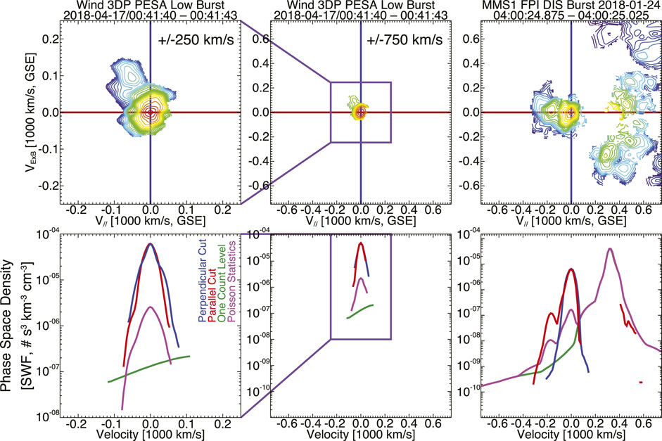
FIGURE 2. Illustrative example ion VDFs from Wind 3DP (Wilson et al., 2021) and MMS DIS (Pollock et al., 2016). The format is similar to that of Figure 1 except there is an extra panel for PESA Low showing the zoomed-in view of the VDF (i.e., first column). All columns show VDFs that have been transformed to the incident core, bulk flow rest frame (i.e., defined by centering the peak phase space density on the origin of this field-aligned coordinate basis).

There is more to examine than just the superficial difference in thermal spread here as well. If one looks closely at the lowest energy (in the core ion rest frame) part of the VDF, specifically the perpendicular cut (blue line) in the left-hand panel, it becomes clear there are effectively two cold populations. When one “zooms out” to a larger velocity range (i.e., middle and right-hand panels), neither 3DP or DIS resolve this colder population⁷. While it may seem like a nuanced issue stuck in the minutiae, this coldest part of the VDF carries the majority of the number density, and thus, the majority of the kinetic energy density. Further, it was known at the time of launch that 3DP would not fully resolve the solar wind core, due to data/telemetry/technological constraints. Thus, even the “zoomed-in” view in the left-hand panels of Figure 2 contain more detail than is currently shown. The instrument does capture what is effectively a proton strahl in the anti-parallel direction (i.e., red line for negative velocities). However, such features are lost in the DIS measurement or the “zoomed-out” view from 3DP. Previous work has shown that treating the VDF as a single population results in a grossly incorrect picture when viewed from velocity moments [e.g., (Wilson et al., 2014a)]. Further, the inability to properly resolve the ion populations precludes us from examining whether any energy is used to “reshape” the VDF, similar to what is seen in electron VDFs [e.g., (Wilson et al., 2020)], versus to heat the VDF. We are also unable to accurately measure any associated skewness or heat flux in the ions for most intervals [e.g., (Scudder, 2015; Schwartz et al., 2022)]. The efficiencies and pathways through which these would occur are different and it is critical we understand them because they are fundamental processes not limited to shock physics.

A recent study (Schwartz et al., 2022) attempted to budget all the energy inputs and outputs across the terrestrial bow shock using MMS to illustrate both its capabilities and limitations. They showed that the limitations of the FPI instruments in the solar wind required their reliance on time-shifted Wind observations (something not unique to this study). They also noted that the inability to properly measure and separate heavy ions like alpha-particles greatly inhibits our ability to properly determine fundamental but basic properties of a plasma, like the equation of state.

In summary, the purpose of this discussion is to illustrate that caution is necessary when using DES and DIS data in the solar wind when the instrument is in burst mode and not in its solar wind energy table mode. This section is also meant to convey that while the MMS FPI detectors are unparalleled in the magnetosheath and magnetosphere, they were not designed for the solar wind and are thus not accurate in that region.

However, a critical lesson we should recognize from MMS observations is that higher resolution measurements can and do result in paradigm shifting discoveries. It is not difficult to see that higher energy, angular, and time resolution measurements in the solar wind near 1 AU would provide substantial advances in our understanding of weakly collisional plasmas. There are fundamental processes at play in the solar wind, in its evolution of the particle VDFs, that are critical to our understanding of kinetic physics and statistical mechanics. Some of these issues, were they to be properly addressed, would reach the level of major physics prizes/awards and could upend the foundations of our conceptual thinking of kinetic physics and its broader implications.

6 Measurements necessary for progress

Recent studies have been performed to examine new technologies and/or new algorithms to improve solar wind observations for future missions [e.g., (De Marco et al., 2016; Cara et al., 2017; De Keyser et al., 2018)]. The mission concept called Turbulent Heating ObserveR or THOR (Vaivads et al., 2016) would have had a thermal particle instrument with an angular resolution of $\sim 3°$ and an energy resolution of ∼5–8%. This would have been the first instrument to properly resolve the ions in the near-Earth solar wind. Unfortunately, THOR was not selected by ESA and is no longer funded. Another mission concept was recently proposed to help address this inability to properly resolve the solar wind ions as well (Borovsky and Raines, 2022).

Table 1 shows direct instrument capabilities comparisons between some current missions and two concepts, THOR and MAKOS. The table is separated into ions and electrons, as the measurements and technological limitations are different for measuring the different species. The table lists the nominal or typical values for the various instruments, taken from the instrument papers or direct observations as for the Wind 3DP detectors. The table lists the cadence (i.e., time between full VDF measurements), energy resolution (ΔE/E), azimuthal angular resolution (Δϕ), poloidal/latitudinal angular resolution (Δθ), and energy range. While Wind was designed to measure the solar wind VDFs, it was greatly limited by technological and telemetry constraints when it was designed and built (compared to modern missions). Even so, as we have shown, it can do much better than some modern missions precisely because it was designed to measure the solar wind. Note we did not show the IMAP instrument comparisons in the table as the instrument papers are not yet published and IMAP is not being designed for in situ science.

TABLE 1

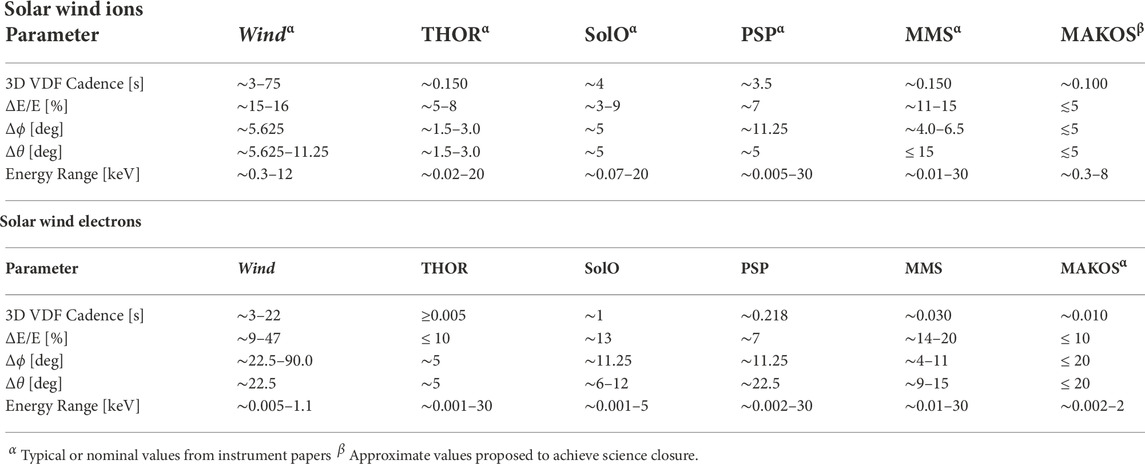
TABLE 1. Instrument comparisons.

The ideal state of the art advancements in solar wind VDF measurements over the next decade would increase time resolutions for full 3D 4π ion distributions in the solar wind down to $<$ 100 ms, with energy resolutions $<$ 5% and angular resolutions $<$ 5°. These values should reduce to $<$ 10 ms with energy resolutions $<$ 2.5% and angular resolutions $<$ 2.5° over the next 3 decades. The justification for such constraints arise from the analysis performed by Cara et al. (2017); De Keyser et al. (2018); De Marco et al. (2016). One can see by examining their simulated reconstruction of the VDFs that even with THOR’s advanced capabilities, we would still not fully resolve some features.

The resolutions referenced above derive from the need to resolve things like fast/magnetosonic-whistler precursors [e.g., (Wilson et al., 2017)] with ion measurements, shock ramps, and short-duration reconnection processes [e.g., (Wang et al., 2020)] with ion and electron measurements. Since many electron-scale fluctuations have spacecraft frame in the 100s–1000s of Hz, there is little hope to provide full 3D VDFs on those time scales. However, many of these phenomena (e.g., lion roars/whistler mode waves, magnetosonic-whistlers, etc.) grow a much slower rates, on the order of the lower hybrid resonance frequency (∼10 Hz in the solar wind near 1 AU). For these phenomena, we do have a finite probability of observing some of their evolution in time from, for instance, an instability [e.g., (Akimoto et al., 1993; Forslund et al., 1970; Forslund et al., 1971; Gary, 1993; Matsukiyo and Scholer, 2006)]. Some previous work has even shown that MMS has sufficient time resolution (but not quite the energy-angular resolution) to observe part of the evolution of shock-reflected ion beams near the bow shock [e.g., (Goodrich et al., 2019)]. There is also the issue of trying to properly resolve the particle VDFs during/within a turbulent region of space. The electric and magnetic fields are often capable of examining down to electron-scales, but the particle data are either too slow or do not properly resolve the VDFs [e.g., see discussion in (Wilson et al., 2021), and references therein].

Electron VDF measurements can have slightly more relaxed energy and angular resolution due to their larger thermal-to-bulk speed ratios. However, the time resolution is a much stricter constraint because electron time scales are so much shorter than any ion time scale. Finally, it is imperative that the lowest energy bin for electron measurements be no more than ∼1–2 eV to ensure the instrument observes photoelectrons for correction/removal (Lavraud and Larson, 2016).

7 Constructing energy distributions

To further illustrate the necessity of improved solar wind measurements, we provide a case example for both ions and electrons. In the following, we will generate a generic, model energy distribution function (EDF) for each population and then interpolate particle instruments to these model EDFs to illustrate the sparsity of measurements. We will also provide an example of a future instrument concept that would address the current measurement deficit (e.g., see the MAKOS science and mission concept white papers submitted to the Heliophysics Decadal Survey led by Prof. Katherine Goodrich).

Note that the purpose of examining these model distributions in this way is to illustrate that without high resolution measurements, even the velocity moments of the entire distribution (i.e., not separating out species or subcomponents) are highly inaccurate. Further, although the MAKOS mission concept intends to use a time-of-flight (ToF) component to its solar wind ion instrument, we do not separate out protons and alpha-particles in Section 7.1.2 so as to directly compare with Wind and MMS.

To start, we define the Maxwell-Boltzmann EDF for a system with three degrees of freedom in the presence of a potential, ϕ_s, is given by:

$f_s\left(E\right)=2n_s\sqrt{\frac{E-{\varphi }_s}{\pi }}{\left(k_B{T}_s\right)}^{-3/2}{e}^{-\left(\frac{E-{\varphi }_s}{k_B{T}_s}\right)}(1)$

where k_B is Boltzmann’s constant, T_s is the temperature, and n_s is the number density of particle species s. Note that unlike a velocity distribution function (VDF), the units of the EDF are given as number per unit volume per unit energy, e.g., # cm⁻³ eV⁻¹. Normally Eq. 1 is shown in the limit where ϕ_s → 0 and then moments of $f_s\left(E\right)$ are integrated over all energies from zero to infinity. However, in this case in the presence of a potential, the moments are given as:

${ϵ}^N\equiv {\int }_{{\varphi }_s}^{\infty }dE{\left(E-{\varphi }_s\right)}^N{f}_s\left(E\right)(2)$

where ϵ^N is the Nth energy moment of $f_s\left(E\right)$. We also note that, in general, the solar wind particle VDFs are not Maxwellian, i.e., even the low energy part of the VDF is better characterized by the more general self-similar VDF [e.g., see (Wilson et al., 2019a; Wilson et al., 2019b; Wilson et al., 2020)]. However, we forego this additional complication for the sake of simplicity since low resolution instruments can only rarely distinguish between Maxwellian and self-similar VDFs.

We can also define the kappa EDF for a system with three kinetic degrees of freedom in the absence of a potential energy [e.g., (Livadiotis, 2015a; Livadiotis, 2015b)] is given by:

$\begin{array}{ll}\hfill f_s\left(E\right)& =\frac{2n_s{E}^{1/2}\mathrm{\Gamma }\left({\kappa }_s+1\right)}{\sqrt{\pi }\mathrm{\Gamma }\left({\kappa }_s-\frac{1}{2}\right)}{\left[\left({\kappa }_s-\frac{3}{2}\right)\left(k_B{T}_s\right)\right]}^{-3/2}\hfill \\ \hfill & \times {\left[1+{\left({\kappa }_s-\frac{3}{2}\right)}^{-1}\left(\frac{E}{k_B{T}_s}\right)\right]}^{-\left({\kappa }_s+1\right)}\hfill \end{array}(3)$

where k_B is Boltzmann’s constant, κ_s is the kappa exponent, T_s is the temperature, and n_s is the number density of particle species s. Eq. 3 assumes that any kinetic energies are given by the Galilean representation, i.e., $E=\frac{m_s}{2}{\left(\mathbf{v}-{\mathbf{v}}_{os}\right)}^2$ where m_s is the mass and v_os is the drift velocity relative to relevant reference frame of v.

7.1 Interpolation to instrument energies

7.1.1 Electrons

Suppose someone wanted to construct model EDFs for electrons and they were given n_s, T_s, κ_s, ϕ_SC (spacecraft potential), and v_os. For the sake of simplicity, let’s assume that v_os are all along the quasi-static magnetic field vector, B_o, and T_‖ = T_⊥. Then to construct a model $f_s\left(E\right)$, one follows these steps:

•Construct an array of energy bin values, E_o (uniform in logarithmic space)

•Shift E_o by Z_sϕ_SC to generate array of shifted energies, E_sh = E_o + Z_sϕ_SC, where Z_s is the charge state (including sign) of particle species, s

•Compute the equivalent energies, E_os, for each v_os offset to create second shifted energy array, E_ss = E_sh−E_os. This is for a Galilean frame transformation, thus why the shift is done in terms of velocity, not energy.

•For Eq. 1, $\left(E-{\varphi }_s\right)\to E_{ss}$ and for Eq. 3, the first energy (i.e., E^−1/2 factor outside of brackets) goes to E_sh and the second energy (i.e., the E inside the brackets) goes to E_ss, per Livadiotis (Livadiotis, 2015b). That is, only one of the energy terms is affected by the energy shift (which is acting as our potential here) due to the finite v_os.

•Compute $f_s\left(E\right)$ for each electron component (e.g., core, halo, and/or strahl) and sum them together, to generate the total electron EDF, $f_e\left(E\right)$ = $f_{ce}\left(E\right)+f_{he}\left(E\right)+f_{be}\left(E\right)$, where E → E_ss as described above.

•Compute a model EDF for the photoelectrons, $f_{ph}\left(E\right)$, using Eq. 1 by performing empirical fits using constraints from previous work [e.g., (Grard, 1973)].

•Sum the total electron and photoelectron EDFs together to get the total model EDF, $f_{\mathrm{m}\mathrm{o}\mathrm{d}}\left(E\right)=f_e\left(E\right)+f_{ph}\left(E\right)$

Now that we have a model EDF⁸ $f_{\mathrm{m}\mathrm{o}\mathrm{d}}\left(E_o\right)$, we can interpolate to the energy bin values of an actual detector/instrument, E_m, and then integrate the result to get moments of the EDF. Note that in doing so, you will want to follow these steps:

•Compute the base-10 logarithm of $f_{\mathrm{m}\mathrm{o}\mathrm{d}}\left(E\right)$ then linearly interpolate to E_m, giving $L_m\left(E_m\right)$

•Convert back to linear space to get the measured EDF, $f_m\left(E_m\right)=10^{L_m\left(E_m\right)}$

Note that $f_m\left(E_m\right)$ is at the unadjusted, spacecraft frame energies, E_m. That is, these energies have not yet accounted for ϕ_SC so keep that in mind. These are the energy bin values of a detector. Thus, when finding the moments of $f_m\left(E_m\right)$, only use the elements of $f_m\left(E_m\right)$ and E_m that satisfy E_m > ϕ_SC (assuming ϕ_SC > 0).

To compute the moments, follow these steps:

•Define the good elements that satisfy E_m > ϕ_SC

•Define the shifted energies, E_msh = E_m − ϕ_SC

•Calculate the number density, n_em, by numerically integrating over $f_m\left(E_m\right)$ with E_msh as the abscissa

•Calculate the temperature, T_em, by numerically integrating over $E_{\mathit{msh}}{f}_m\left(E_m\right)$ with E_msh as the abscissa, then multiplying by $\frac{2}{3n_{em}}$ (i.e., mean kinetic energy is defined as $\frac{3}{2}{n}_{em}{T}_{em}$, where T_em is in units of energy)

One can compare the results by numerically integrating $f_{\mathrm{m}\mathrm{o}\mathrm{d}}\left(E\right)$ in a similar manner with E_ss as the abscissa and multiplying factor. Typically, one can use E_sh instead of E_ss because the electron fit parameters are often defined in the solar wind bulk flow rest frame where j = − e ∑_sn_s v_os ≃ 0 (i.e., the effective offset should be zero after accounting for the spacecraft potential because the sub-offsets used to construct the three electron components should balance).

We construct a regular energy grid in logarithmic space to increase the density of points at lower energies where things change much more quickly to generate the initial $f_{\mathrm{m}\mathrm{o}\mathrm{d}}\left(E\right)$. We then follow the above steps to calculate $f_m\left(E_m\right)$ at energy bin values of Wind’s EESA Low $(f_{EL}\left(E_{EL}\right))$, MMS’s DES $(f_{\mathit{DES}}\left(E_{\mathit{DES}}\right))$, and a concept instrument for the potential future MAKOS mission $(f_{\mathit{MAK}}\left(E_{\mathit{MAK}}\right))$. We numerically compute the energy moments using Simpson’s 1/3 rule [e.g., see discussion in (Wilson et al., 2019b)] of $f_{\mathrm{m}\mathrm{o}\mathrm{d}}\left(E\right)$ and compare those results to the numerical moments of $f_{EL}\left(E_{EL}\right)$, $f_{\mathit{DES}}\left(E_{\mathit{DES}}\right)$, and $f_{\mathit{MAK}}\left(E_{\mathit{MAK}}\right)$.

As an example, we used a model distribution with the following parameters [taken from (Wilson et al., 2019a; Wilson et al., 2019b; Wilson et al., 2020)] for the perpendicular direction, assuming an isotropic distribution (i.e., for simplicity to avoid any issues with v_os):

•Prescribed Model Parameters

•n_ec(h)[b] ∼ 8.29(0.27)[0.16] cm⁻³

•T_ec(h)[b] ∼ 12.91(47.66)[37.41] eV

•κ_eh[b] ∼ 4.10[3.84] N/A

•ϕ_SC ∼ 7.42 eV

•Prescribed Photoelectron Model Parameters

•n_ph ∼ 104.9 cm⁻³

•T_ph ∼ 0.6695 eV

•ϕ_ph ∼ 2.24 eV⁹

Figure 3 shows the example model electron EDF (solid red lines) and the interpolated data points at each instrument energy (color-coded symbols). These are for the nominal mid-point energy bins of each instrument. The vertical (orange) dashed line shows the location of ϕ_SC and the cyan line shows the photoelectron EDF.

FIGURE 3

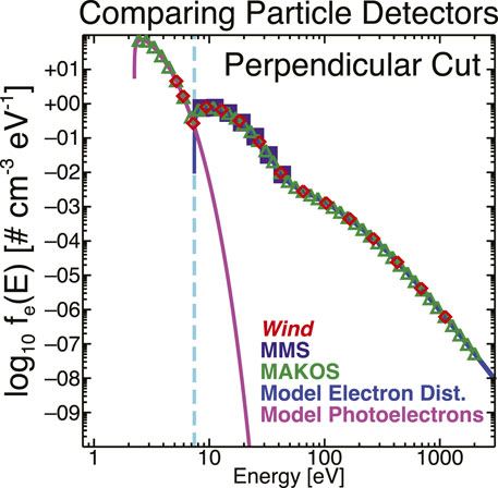
FIGURE 3. Example of the model EDF for the case where T_ec ∼ 5.025 eV. The solid magenta (photoelectron model) and blue (ambient electron model) illustrate the model to which the instrument energy bins are interpolated. Three instruments are shown from Wind (red diamonds), MMS (purple squares), and the mission concept MAKOS (green triangles). The instrument energy bins are discussed in more detail in Section 7.1.1.

One should immediately note that there are very few MMS DES energy bins shown in Figure 3. As can be seen in Figure 1, there are substantial regions of velocity space where the MMS DES detector has extremely low signal-to-noise (SNR) ratios, i.e., the data are not statistically significant. To get a proxy for the statistically significant energy bins, we examined the MMS DES VDFs in a burst interval on 2018-01-24 where the MMS1 spacecraft was in the solar wind¹⁰ (i.e., we exclude the first part of the interval “contaminated” by shock-reflected particles). We use the SPEDAS (Angelopoulos et al., 2019) software to retrieve the MMS DES data and we use their built-in routines to remove the secondary electron errors. We then adjust for the spacecraft potential and an example of the end result is seen in Figure 1. We then calculate the ratio between this corrected data and the Poisson statistics, $\frac{\delta f}{f}$, of the corrected data for all VDFs in the interval and all energy-angle bins. Note that in burst mode, the DES instrument measures 32 energies, 16 poloidal angles, and 32 azimuthal angles, i.e., 16,384 energy-angle bins per VDF. In contrast, Wind EL has 15 energies and 88 angle bins for a total of 1,320 energy-angle bins.

The MMS DES data are returned as a 4D array of data, i.e., [V,E,T,P]-elements where V is the number of VDFs, E is the number of energy bins, T is the number of poloidal bins, and P is the number of azimuthal bins. We average $\frac{\delta f}{f}$ over the V VDFs and then determine how many of these energy-angle bins satisfy ≥0.5. If the number is at least 200, then we consider it a good energy bin, otherwise not. The “good” DES energy bins are:

E [eV]: 8.54, 11.2, 14.6, 19.2, 25.1, 32.8, and 43.0.

That is, there are only 7 energy bins that consistently have enough SNR to be statistically significant for DES when it is in burst mode in the solar wind (for this interval). Performing the same calculations for Wind EL shows that all 15 energy bins are consistently valid for 3 days worth of data¹¹. The Wind EL energies are:

E [eV]: 5.18, 5.92, 7.26, 9.41, 12.8, 18.3, 27.3, 41.8, 65.2, 103, 165, 265, 427, 689, and 1,113.

The instrument concept for MAKOS (as of Aug. 2022) includes a dedicated, low energy (∼1–2000 eV) electron and ion (∼400–6,000 eV) instrument designed to measure the solar wind. The electron(ion) instrument is planned to have ΔE/E ∼ 15%(7%) and Δα < 15°(6°). To determine the number of energy bins, N, based upon the energy range, $\left[E_{\min },E_{\max }\right]$, and ΔE/E, one can show that:

$\left(N-1\right)=\frac{{\log }_{10}{E}_{\max }-{\log }_{10}{E}_{\min }}{{\log }_{10}|2+\frac{\mathrm{\Delta }E}{E}|-{\log }_{10}|2-\frac{\mathrm{\Delta }E}{E}|}(4)$

Therefore, the electron(ion) instrument will need at least 52(40) energy bins. These will most likely be on a uniform grid in logarithmic space. Because we cannot know ahead of time which energy bins will have sufficient counting statistics for this analysis, we use the full array.

Note that the accuracy of the results depends upon the actual location of the discrete energy values and the range of energy values¹². For instance, one can get a more accurate numerical integration result with a lower energy grid resolution if the lowest energy is closer to E_sh ∼ 0 than another grid with higher resolution but also a higher minimum energy bin value. Therefore, to test the stability of our integration we perturb the instrument energies. We construct an array of perturbing values between ±2 eV and integrate the resulting interpolated instrument EDF, $f_m\left(E_m\right)$. This provides us with an array of possible moment values on which to perform simple one-variable statistics. We define the percent difference as $Q_{\%}=\left(1-\frac{Q_m}{Q_{\mathrm{m}\mathrm{o}\mathrm{d}}}\right)\times 100\%$, where Q_m is the moment of the EDFs interpolated to the instrument energies and Q_mod is the moment of model EDF. We report the results as X_5%(X_95%)($\tilde{X}$), where X_j% is the j^th percentile and $\tilde{X}$ is the median. We further illustrate the issue of moment accuracy by adding two additional examples but change only T_ec for the model to 5 eV and 25 eV (i.e., representative cold and hot electrons in the solar wind). The results are summarized in Table 2.

TABLE 2

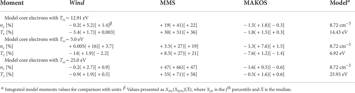
TABLE 2. Electron velocity moment accuracy.

Thus, it becomes quite clear that both Wind and MAKOS do significantly better than MMS. This should be expected, as both Wind and MAKOS are/will be designed for the solar wind. There are also rather significant improvements in the accuracy of the results using an irregularly spaced energy grid than the uniform in linear space results shown in Section 7.1. The reason being that even when the solar wind is considered “hot” as in our third example here, the distribution is still much cooler than typical magnetosheath and/or magnetosphere plasmas. Further, the instrument often has rather low SNR in the solar wind, which means only a small subset of all possible energy bins are actually valid in the solar wind.

Note that if the instrument cannot accurately represent the velocity moments of an entire VDF, it is extremely unlikely that one can separate out the subpopulations and/or species. For instance, the median uncertainty in n_e and T_e for each of the MMS calculations in Table 2 are ≳19% and ≳21%, respectively. The purpose of these example calculations are to illustrate that even in the most superficial analysis, we are missing a great deal if we use low resolution instrumentation. One can see that MMS only has a few energy bins at most in the halo and strahl energy ranges, which means there is no hope of modeling those populations. Again, this is not surprising as the FPI instrument on MMS was not designed for the solar wind. This is not a denigration of FPI but rather a note of caution to illustrate the limitations and need for higher resolution instrumentation.

7.1.2 Ions

We follow a similar series of steps as in Section 7.1.1 to construct a model ion EDF. Here we use the model distribution described by Eq. 1 with typical parameters [taken from 76] for the protons and alpha-particles. Because most instruments measure energy per charge, we construct the EDFs in terms of speed of protons (i.e., convert from energy to speed assuming proton mass) and then convert back into energy space after drift speeds (relative to spacecraft frame), v_os, are taken into account. Again, we use the actual midpoint energy bin values of Wind’s PESA Low Burst $(f_{PL}\left(E_{PL}\right))$, MMS’s DIS $(f_{\mathit{DIS}}\left(E_{\mathit{DIS}}\right))$, and a concept instrument for the potential future MAKOS mission $(f_{\mathit{MAK}}\left(E_{\mathit{MAK}}\right))$. Note that the mission concept for MAKOS will include a ToF component to the solar wind ion instrument, which would allow it to separate protons and alpha-particles. However, for direct comparison, we only examine the effect of the higher energy resolution.

Note that the typical mid-point energies for PL are:

E [eV]: ∼670, 786, 922, 1,079, 1,265, 1,485, 1740, 2037, 2,384, 2,797, 3,278, 3,837, 4,495, 5,264.

Similar to how we limited the DES “good” energy bins, we considered the statistical averages over an array of DIS VDFs in the solar wind. However, the threshold for $\frac{\delta f}{f}$ here was 0.1 and only 10 angle bins needed to satisfy this requirement (i.e., because the ion VDF is much more narrow in energy-angle space than the electrons). The “good” DIS energy bins are:

E [eV]: ∼556, 736, 975, 1,291, 1709, 2,263, 2,997, 3,968, 5,253, 6,955.

The instrument concept for MAKOS (as of Aug. 2022) includes a dedicated, low energy ion (∼300–8,000 eV) instrument designed to measure the solar wind. The ion instrument is planned to have ΔE/E ∼ 7% and Δα < 6°. Using Eq. 4 we can show we need at least 40 logarithmically spaced energy bins to achieve these parameters. Similar to the electron MAKOS instrument, because we cannot know ahead of time which energy bins will have sufficient counting statistics for this analysis, we use the full array.

Figure 4 is similar to Figure 3 but here there are no photoelectrons and the spacecraft potential is negligible compared to the incident (on the instrument in the spacecraft frame) ion kinetic energies. The solid blue line shows the model ion EDF where we have summed the proton and alpha-particle contributions as they would be observed by an instrument without a time-of-flight capability (i.e., one cannot directly separate protons from alpha-particles so the EDF contains all ions).

FIGURE 4

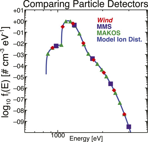
FIGURE 4. Example of the model EDF for the ions. The format is the same as in Figure 3 but here we do not have photoelectrons or a vertical line to mark the spacecraft potential.

We numerically integrated this model ion EDF and perturbed the instrument energy bins as was discussed in Section 7.1.1. Again, we report the one-variable statistics of the results as X_5%(X_95%)($\tilde{X}$), where X_j% is the j^th percentile and $\tilde{X}$ is the median. Similar to Section 7.1.1 we provide example comparison for three different models. The first model is described below and the subsequent two only change T_p to 10 eV and 20 eV, respectively.

•Prescribed Model Parameters

•n_p[α] ∼ 11.7[0.53] cm⁻³

•T_p[α] ∼ 5.43[34.7] eV

•${\mathbf{v}}_{op}\sim \left(-450,-7.22,-21.1\right)$ km/s, GSE

•${\mathbf{v}}_{o\alpha }\sim \left(-400,-0.83,-5.28\right)$ km/s, GSE

Table 3 follows the same format as Table 2 but for the ions, where the integration assumes a single ion population (i.e., since as stated earlier, most instruments only measure energy per charge). Again, we can see that the MMS instrument suffers large uncertainties but as we stated before, this is to be expected. The FPI instrument was not designed to measure the cold, fast solar wind distributions.

TABLE 3

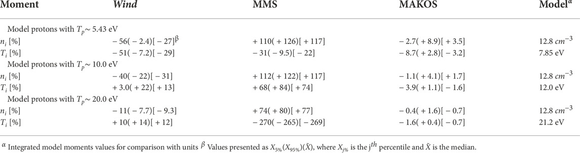
TABLE 3. Ion velocity moment accuracy.

The future MAKOS instrument performs very well, as one would expect. Both the density and temperature estimates are significantly better than both the Wind and MMS results. Note that the MAKOS density is only off from the true number density of 12.75 cm⁻³ by roughly a few percent.

There are several major things to consider here. The first is that much of the literature will report uncertainties in terms of an idealized, statistical uncertainty (i.e., they do not account for errors/uncertainties in instrument calibration etc.). These are nearly always much smaller than the total uncertainty of any given measurement. The second is that the above results for both the ions and electrons are kind of a worst case scenario to illustrate the difference that detector design can have on measured distributions. In practical implementation of any electrostatic analyzer (ESA), the distribution is not integrated over just energy as has been done here. There are geometric factor corrections, deadtime corrections, efficiency corrections, angular corrections, etc. All of these corrections actually improve the results from those presented here, which is why, for example, Wind’s velocity moments are not off by upwards of 30–50% just because the solar wind is cold.

Again, much like with the electrons, the large uncertainties resulting from low resolution measurements precludes our ability to properly separate ion species and even subpopulations [e.g., secondary proton beam (Alterman et al., 2018)]. Further, the solar wind core protons are often cold, i.e., T_p < 10 eV [e.g., (Wilson et al., 2018)], which presents the biggest issue for accurately capturing the total number density from numerical velocity moments calculated from low resolution measurements, but less so for a temperature estimate, unexpectedly. The sparsity of energy bins in low resolution measurements presents a sort of numerical instability whereby the uncertainties fluctuate wildly by varying only one parameter, like T_p as done here. This should cause pause in anyone using velocity moments in the solar wind from instruments designed for the magnetosphere or instruments with insufficient resolution. This is not to say that all solar wind data from such instruments are useless, as illustrated by Artemyev et al. (Artemyev et al., 2018) and Roberts et al. (Roberts et al., 2021). Rather, the purpose is to illustrate that caution should be taken and better instrumentation is necessary to properly address this issue. Inaccurate velocity moments can affect our interpretation of results from instability analysis to model input parameters for simulations, thus better instrumentation is clearly necessary.

8 Summary and conclusion

The purpose of this article is to illustrate that high resolution particle VDF measurements are an essential requirement for any in situ mission. We also show that although MMS is unparalleled in the magnetosphere and magnetosheath for measuring particle VDFs, it does not perform well in the solar wind (as it was not designed for this region of space). PSP and SolO have high resolution particle VDFs, but neither are near 1 AU and both have their own limitations and issues (e.g., heat shield obscures the ion VDFs for much of PSPs orbit). The focus of the future IMAP mission is not in situ science, so its particle instruments will be largely focused on providing velocity moments for space weather purposes. There is hope with plans to design and build the potential future mission currently called HelioSwarm (Klein et al., 2019) but the instrument specifics are still not published. We also hope that this article will motivate further studies to critically examine the limitations of relying upon velocity moments from under resolved VDF measurements and/or other instrumental/measurement limitations.

A critical examination of the core proton population could show as much diversity as the electron distributions below ∼1 keV, which would completely change our understanding of the solar wind and how it evolves. PSP is conveniently measuring very slow solar wind during its perihelion passes, which improves the velocity resolution measurements in the core of the solar protons. As such, they are seeing a great deal of structure in the ion VDFs that we just cannot resolve¹³ at 1 AU [e.g., (Verniero et al., 2020)]. Multiple populations, multiple species, and numerous non-Maxwellian features all result in vastly different instabilities [e.g., (Chen et al., 2016; Husidic et al., 2020; Verniero et al., 2020; Klein et al., 2021)] and particle dynamics at boundaries like shocks or current sheets [e.g., (Gedalin and Ganushkina, 2022; Ha et al., 2022)]. All of these phenomena can greatly alter the evolution of the solar wind, since all are tied to its acceleration and propagation away from the Sun. Therefore, it is critical we properly resolve all the populations if we are to understand the acceleration and evolution of the solar wind, among numerous other kinetic physics topics of interest.

Since all the interesting, fundamental processes of interest to plasma physicists occur at collisionless shocks (e.g., reconnection, turbulence, particle acceleration, wave-particle interactions), it is particularly relevant to have proper solar wind measurements for such investigations. It is also critical that we design a mission focused on examining collisionless shocks to advance our understanding of these fundamental topics (e.g., see the MAKOS mission concept led by Prof. Katherine Goodrich).

Without such measurement advancements, we will not reach closure on multiple major topics such as wave-particle interactions, turbulence dissipation, energy dissipation in collisionless shocks, and particle acceleration by waves and/or shocks. All of these topics have implications for nonequilibrium statistical mechanics, plasma physics, and astrophysics.

Data availability statement

The original contributions presented in the study are included in the article/supplementary material, further inquiries can be directed to the corresponding author.

Author contributions

All authors listed have made a substantial, direct, and intellectual contribution to the work and approved it for publication.

Funding

LW was partially supported by Wind MO&DA funds and a NASA ROSES HMCS grant (civil servants are not assigned grant numbers). KG, DT, PW, and SS were partially supported by NASA ROSES HMCS grant 80NSSC22K0111.

Acknowledgments

The authors would like to thank the Southwest Research Institute engineering team for useful feedback on some aspects of future instrumentation. We would also like to thank K.G. Klein, J.M. TenBarge, D. Verscharen, and J.S. Halekas for discussions of solar wind measurements and instabilities.

Conflict of interest

The authors declare that the research was conducted in the absence of any commercial or financial relationships that could be construed as a potential conflict of interest.

Publisher’s note

All claims expressed in this article are solely those of the authors and do not necessarily represent those of their affiliated organizations, or those of the publisher, the editors and the reviewers. Any product that may be evaluated in this article, or claim that may be made by its manufacturer, is not guaranteed or endorsed by the publisher.

Footnotes

¹A plasma instability is “…the mechanism through which a plasma converts some particle free energy source into electromagnetic fluctuations … ” (Wilson et al., 2021).

²Note that the ions can carry a non-negligible heat flux in the solar wind (Hellinger et al., 2011; Hellinger et al., 2013; Scudder, 2015).

³The idea that particle velocities are uncorrelated.

⁴Note that higher time resolutions are possible for PSP [personal communication with instrument team, circa 2020].

⁵statistically for this outbound bow shock pass, only 7 of the 32 energy bins had sufficient counts.

⁶Note that the observations in both Figures 1, 2 are constructed using a 3D Delaunay tetrahedralization to re-grid the data (after corrections for spacecraft potential and frame transformations), i.e., these are not direct measurements.

⁷Note that if we “zoom-in” the velocity range for MMS, we still would not resolve the two cold populations seen by Wind. In the “zoomed-out” view, one can see that MMS does not even properly resolve the hotter of the two populations.

⁸Note that when interpolating to the E_m values, the abscissa of $f_{\mathrm{m}\mathrm{o}\mathrm{d}}\left(E\right)$ need to be the original energy grid values, E_o. This is because the instrument E_m values have not been corrected for ϕ_SC or any distribution offsets, i.e., they are the unadjusted spacecraft frame energies.

⁹Note that ϕ_ph is just a fit parameter value from the model function, not necessarily a physically representative estimate of ϕ_SC. The issue arises from there only being two or three energy bins below ϕ_SC, so the fit is under-constrained.

¹⁰The interval used spans 2018-01-24/04:00:40.0000 UTC to 2018-01-24/04:01:50.0000 UTC which corresponds to 2333 DES VDFs.

¹¹It is worth noting, again, that the MMS instruments were not designed for the cold, fast solar wind. The Wind 3DP instrument was and it integrates over ∼3 s, ∼100 times longer than MMS DES. Thus, it is not surprising that MMS has low SNR in the solar wind. However, it is incredibly important to consider this and know about the implications.

¹²It is actually more complicated than this, see https://math.stackexchange.com/a/1599401/177342 for example.

¹³It is also possible these features do not exist in the near-Earth solar wind but we cannot know due to insufficient measurement resolution.

References

Akimoto, K., Winske, D., Gary, S. P., and Thomsen, M. F. (1993). Nonlinear evolution of electromagnetic ion beam instabilities. J. Geophys. Res. 98, 1419–1433. doi:10.1029/92JA02345

CrossRef Full Text | Google Scholar

Alterman, B. L., Kasper, J. C., Stevens, M. L., and Koval, A. (2018). A comparison of alpha particle and proton beam differential flows in collisionally young solar wind. Astrophys. J. 864, 112. doi:10.3847/1538-4357/aad23f

CrossRef Full Text | Google Scholar

Alvarez Laguna, A., Esteves, B., Bourdon, A., and Chabert, P. (2022). A regularized high-order moment model to capture non-Maxwellian electron energy distribution function effects in partially ionized plasmas. Phys. Plasmas 29, 083507. doi:10.1063/5.0095019

CrossRef Full Text | Google Scholar

Angelopoulos, V., Cruce, P., Drozdov, A., Grimes, E. W., Hatzigeorgiu, N., King, D. A., et al. (2019). The space physics environment data analysis system (SPEDAS). Space Sci. Rev. 215, 9. doi:10.1007/s11214-018-0576-4

PubMed Abstract | CrossRef Full Text | Google Scholar

Argall, M. R., Barbhuiya, M. H., Cassak, P. A., Wang, S., Shuster, J., Liang, H., et al. (2022). Theory, observations, and simulations of kinetic entropy in a magnetotail electron diffusion region. Phys. Plasmas 29, 022902. doi:10.1063/5.0073248

CrossRef Full Text | Google Scholar

Artemyev, A. V., Angelopoulos, V., and McTiernan, J. M. (2018). Near-earth solar wind: Plasma characteristics from ARTEMIS measurements. JGR. Space Phys. 123, 9955–9962. doi:10.1029/2018JA025904

CrossRef Full Text | Google Scholar

Bhatnagar, P. L., Gross, E. P., and Krook, M. (1954). A model for collision processes in gases. I. Small amplitude processes in charged and neutral one-component systems. Phys. Rev. 94, 511–525. doi:10.1103/PhysRev.94.511

CrossRef Full Text | Google Scholar

Borovsky, J. E., and Raines, J. M. (2022). Heliospheric structure analyzer (hsa): A simple 1-AU mission concept focusing on large-geometric-factor measurements. Front. Astron. Space Sci. 9, 919755. doi:10.3389/fspas.2022.919755

CrossRef Full Text | Google Scholar

Cara, A., Lavraud, B., Fedorov, A., De Keyser, J., DeMarco, R., Marcucci, M. F., et al. (2017). Electrostatic analyzer design for solar wind proton measurements with high temporal, energy, and angular resolutions. J. Geophys. Res. Space Phys. 122, 1439–1450. doi:10.1002/2016JA023269

CrossRef Full Text | Google Scholar

Chen, C. H. K., Matteini, L., Schekochihin, A. A., Stevens, M. L., Salem, C. S., Maruca, B. A., et al. (2016). Multi-species measurements of the firehose and mirror instability thresholds in the solar wind. Astrophys. J. 825, L26. doi:10.3847/2041-8205/825/2/L26

CrossRef Full Text | Google Scholar

De Keyser, J., Lavraud, B., Přech, L., Neefs, E., Berkenbosch, S., Beeckman, B., et al. (2018). Beam tracking strategies for fast acquisition of solar wind velocity distribution functions with high energy and angular resolutions. Ann. Geophys. 36, 1285–1302. doi:10.5194/angeo-36-1285-2018

CrossRef Full Text | Google Scholar

De Marco, R., Marcucci, M. F., Bruno, R., D'Amicis, R., Servidio, S., Valentini, F., et al. (2016). Importance of energy and angular resolutions in top-hat electrostatic analysers for solar wind proton measurements. J. Instrum. 11, C08010. doi:10.1088/1748-0221/11/08/C08010

CrossRef Full Text | Google Scholar

Dum, C. T., Chodura, R., and Biskamp, D. (1974). Turbulent heating and quenching of the ion sound instability. Phys. Rev. Lett. 32, 1231–1234. doi:10.1103/PhysRevLett.32.1231

CrossRef Full Text | Google Scholar

Dum, C. T. (1975). Strong-turbulence theory and the transition from landau to collisional damping. Phys. Rev. Lett. 35, 947–950. doi:10.1103/PhysRevLett.35.947

CrossRef Full Text | Google Scholar

Forslund, D. W., Morse, R. L., and Nielson, C. W. (1970). Electron cyclotron drift instability. Phys. Rev. Lett. 25, 1266–1270. doi:10.1103/PhysRevLett.25.1266

CrossRef Full Text | Google Scholar

Forslund, D. W., Morse, R. L., and Nielson, C. W. (1971). Nonlinear electron-cyclotron drift instability and turbulence. Phys. Rev. Lett. 27, 1424–1428. doi:10.1103/PhysRevLett.27.1424

CrossRef Full Text | Google Scholar

Gary, S. P. (1993). Theory of space plasma microinstabilities, cambridge atmospheric and space science series. Cambridge, UK: Cambridge University Press.

Google Scholar

Gedalin, M., and Ganushkina, N. (2022). Different heating of Maxwellian and kappa distributions at shocks. J. Plasma Phys. 88, 905880501. doi:10.1017/S0022377822000824

CrossRef Full Text | Google Scholar

Gershman, D. J., Avanov, L. A., Boardsen, S. A., Dorelli, J. C., Gliese, U., Barrie, A. C., et al. (2017). Spacecraft and instrument photoelectrons measured by the dual electron spectrometers on MMS. JGR. Space Phys. 122, 11548. doi:10.1002/2017JA024518

CrossRef Full Text | Google Scholar

Goldman, M. V., Newman, D. L., and Mangeney, A. (2007). Theory of weak bipolar fields and electron holes with applications to space plasmas. Phys. Rev. Lett. 99, 145002. doi:10.1103/PhysRevLett.99.145002

PubMed Abstract | CrossRef Full Text | Google Scholar

Goldman, M. V., Newman, D. L., Eastwood, J. P., and Lapenta, G. (2020). Multibeam energy moments of multibeam particle velocity distributions. JGR. Space Phys. 125, e2020JA028340. doi:10.1029/2020JA028340

CrossRef Full Text | Google Scholar

Goldman, M. V., Newman, D. L., Eastwood, J. P., Lapenta, G., Burch, J. L., and Giles, B. (2021). Multi-beam energy moments of measured compound ion velocity distributions. Phys. Plasmas 28, 102305. doi:10.1063/5.0063431

CrossRef Full Text | Google Scholar

Goodrich, K. A., Ergun, R. E., Schwartz, S. J., Wilson, L. B., Johlander, A., Newman, D., et al. (2019). Impulsively reflected ions: A plausible mechanism for ion acoustic wave growth in collisionless shocks. J. Geophys. Res. Space Phys. 124, 1855–1865. doi:10.1029/2018JA026436

CrossRef Full Text | Google Scholar

Grard, R. J. L. (1973). Properties of the satellite photoelectron sheath derived from photoemission laboratory measurements. J. Geophys. Res. 78, 2885–2906. doi:10.1029/JA078i016p02885

CrossRef Full Text | Google Scholar

Gressman, P. T., and Strain, R. M. (2010). Global classical solutions of the Boltzmann equation with long-range interactions. Proc. Natl. Acad. Sci. U. S. A. 107, 5744–5749. doi:10.1073/pnas.1001185107

PubMed Abstract | CrossRef Full Text | Google Scholar

Ha, J.-H., Ryu, D., Kang, H., and Kim, S. (2022). Electron preacceleration at weak quasi-perpendicular intracluster shocks: Effects of preexisting nonthermal electrons. Astrophys. J. 925, 88. doi:10.3847/1538-4357/ac3bc0

CrossRef Full Text | Google Scholar

Hellinger, P., Matteini, L., Štverák, v., Trávníček, P. M., and Marsch, E. (2011). Heating and cooling of protons in the fast solar wind between 0.3 and 1 AU: Helios revisited. J. Geophys. Res. 116, 9105. doi:10.1029/2011JA016674

CrossRef Full Text | Google Scholar

Hellinger, P., TráVníček, P. M., Štverák, Š., Matteini, L., and Velli, M. (2013). Proton thermal energetics in the solar wind: Helios reloaded. J. Geophys. Res. Space Phys. 118, 1351–1365. doi:10.1002/jgra.50107

CrossRef Full Text | Google Scholar

Husidic, E., Lazar, M., Fichtner, H., Scherer, K., and Astfalk, P. (2020). Linear dispersion theory of parallel electromagnetic modes for regularized Kappa-distributions. Phys. Plasmas 27, 042110. doi:10.1063/1.5145181

CrossRef Full Text | Google Scholar

Kasper, J. C., Maruca, B. A., Stevens, M. L., and Zaslavsky, A. (2013). Sensitive test for ion-cyclotron resonant heating in the solar wind. Phys. Rev. Lett. 110, 091102. doi:10.1103/PhysRevLett.110.091102

PubMed Abstract | CrossRef Full Text | Google Scholar

Kasper, J. C., Abiad, R., Austin, G., Balat-Pichelin, M., Bale, S. D., Belcher, J. W., et al. (2016). Solar wind electrons alphas and protons (SWEAP) investigation: Design of the solar wind and coronal plasma instrument suite for solar Probe plus. Space Sci. Rev. 204, 131–186. doi:10.1007/s11214-015-0206-3

CrossRef Full Text | Google Scholar

Klein, K. G., Alexandrova, O., and Bookbinder, J. (2019). Direct measurement of the solar-wind taylor microscale using MMS turbulence campaign data. arXiv e-prints, arXiv:1903.05740

Google Scholar

Klein, K. G., Verniero, J. L., Alterman, B., Bale, S., Case, A., Kasper, J. C., et al. (2021). Inferred linear stability of parker solar Probe observations using one- and two-component proton distributions. Astrophys. J. 909, 7. doi:10.3847/1538-4357/abd7a0

CrossRef Full Text | Google Scholar

Lavraud, B., and Larson, D. E. (2016). Correcting moments of in situ particle distribution functions for spacecraft electrostatic charging. J. Geophys. Res. Space Phys. 121, 8462–8474. doi:10.1002/2016JA022591

CrossRef Full Text | Google Scholar

Lazar, M., Yoon, P. H., and Schlickeiser, R. (2012). Spontaneous electromagnetic fluctuations in unmagnetized plasmas. III. Generalized Kappa distributions. Phys. Plasmas 19, 122108. doi:10.1063/1.4769308

CrossRef Full Text | Google Scholar

Lazar, M., Poedts, S., and Michno, M. J. (2013). Electromagnetic electron whistler-cyclotron instability in bi-Kappa distributed plasmas. Astron. Astrophys. 554, A64. doi:10.1051/0004-6361/201220550

CrossRef Full Text | Google Scholar

Lazar, M., Poedts, S., and Schlickeiser, R. (2014). The interplay of Kappa and core populations in the solar wind: Electromagnetic electron cyclotron instability. J. Geophys. Res. Space Phys. 119, 9395–9406. doi:10.1002/2014JA020668

CrossRef Full Text | Google Scholar

Lazar, M., Pierrard, V., Shaaban, S. M., Fichtner, H., and Poedts, S. (2017). Dual maxwellian-kappa modeling of the solar wind electrons: New clues on the temperature of kappa populations. Astron. Astrophys. 602, 602A44. doi:10.1051/0004-6361/201630194

CrossRef Full Text | Google Scholar

Lazar, M., Kim, S., López, R. A., Yoon, P. H., Schlickeiser, R., and Poedts, S. (2018). Suprathermal spontaneous emissions inκ-distributed plasmas. Astrophys. J. 868, L25. doi:10.3847/2041-8213/aaefec

CrossRef Full Text | Google Scholar

Lazar, M., López, R. A., Shaaban, S. M., Poedts, S., and Fichtner, H. (2019). Whistler instability stimulated by the suprathermal electrons present in space plasmas. Astrophys. Space Sci. 364, 171. doi:10.1007/s10509-019-3661-6

CrossRef Full Text | Google Scholar

Lee, S.-Y., Lee, E., and Yoon, P. H. (2019). Nonlinear development of electron heat flux instability: Particle in cell simulation. Astrophys. J. 876, 117. doi:10.3847/1538-4357/ab12db

CrossRef Full Text | Google Scholar

Livadiotis, G. (2015a). Introduction to special section on origins and properties of kappa distributions: Statistical background and properties of kappa distributions in space plasmas. J. Geophys. Res. Space Phys. 120, 1607–1619. doi:10.1002/2014JA020825

CrossRef Full Text | Google Scholar

Livadiotis, G. (2015b). Kappa distribution in the presence of a potential energy. J. Geophys. Res. 120, 880. doi:10.1002/2014JA020671

CrossRef Full Text | Google Scholar

Martin, P. A., and Piasecki, J. (1999). Lorentz's model with dissipative collisions. Phys. A Stat. Mech. its Appl. 265, 19–27. doi:10.1016/S0378-4371(98)90541-6

CrossRef Full Text | Google Scholar

Martinović, M. M., Klein, K. G., Kasper, J. C., Case, A. W., Korreck, K. E., Larson, D., et al. (2020). The enhancement of proton stochastic heating in the near-sun solar wind. Astrophys. J. Suppl. Ser. 246, 30. doi:10.3847/1538-4365/ab527f

CrossRef Full Text | Google Scholar

Maruca, B. A., Kasper, J. C., and Gary, S. P. (2012). Astrophys. J. 748, 137. doi:10.1088/0004-637X/748/2/137

CrossRef Full Text

Maruca, B. A., Bale, S. D., Sorriso-Valvo, L., Kasper, J. C., and Stevens, M. L. (2013). Collisional thermalization of hydrogen and helium in solar-wind plasma. Phys. Rev. Lett. 111, 241101. doi:10.1103/PhysRevLett.111.241101

PubMed Abstract | CrossRef Full Text | Google Scholar

Matsukiyo, S., and Scholer, M. (2006). On microinstabilities in the foot of high Mach number perpendicular shocks. J. Geophys. Res. 111, A06104. doi:10.1029/2005JA011409

CrossRef Full Text | Google Scholar

Matyka, M., Gołembiewski, J., and Koza, Z. (2016). Power-exponential velocity distributions in disordered porous media. Phys. Rev. E 93, 013110. doi:10.1103/PhysRevE.93.013110

PubMed Abstract | CrossRef Full Text | Google Scholar

McComas, D. J., Christian, E. R., Schwadron, N. A., Fox, N., Westlake, J., Allegrini, F., et al. (2018). Interstellar mapping and acceleration Probe (IMAP): A new NASA mission. Space Sci. Rev. 214, 116. doi:10.1007/s11214-018-0550-1

CrossRef Full Text | Google Scholar

McFadden, J. P., Carlson, C. W., Larson, D., Bonnell, J., Mozer, F., Angelopoulos, V., et al. (2008a). THEMIS ESA first science results and performance issues. Space Sci. Rev. 141, 477–508. doi:10.1007/s11214-008-9433-1

CrossRef Full Text | Google Scholar

McFadden, J. P., Carlson, C. W., Larson, D., Ludlam, M., Abiad, R., Elliott, B., et al. (2008b). The THEMIS ESA plasma instrument and in-flight calibration. Space Sci. Rev. 141, 277–302. doi:10.1007/s11214-008-9440-2

CrossRef Full Text | Google Scholar

Nicolaou, G., Verscharen, D., Wicks, R. T., and Owen, C. (2019). The impact of turbulent solar wind fluctuations on solar orbiter plasma proton measurements. Astrophys. J. 886, 101. doi:10.3847/1538-4357/ab48e3

CrossRef Full Text | Google Scholar

Pollock, C., Moore, T., Jacques, A., Burch, J., Gliese, U., Saito, Y., et al. (2016). Fast plasma investigation for magnetospheric multiscale. Space Sci. Rev. 199, 331–406. doi:10.1007/s11214-016-0245-4

CrossRef Full Text | Google Scholar

Roberts, O. W., Nakamura, R., Coffey, V. N., Gershman, D. J., Volwerk, M., Varsani, A., et al. (2021). A study of the solar wind ion and electron measurements from the magnetospheric multiscale mission's fast plasma investigation. JGR. Space Phys. 126, e22021JA029784. doi:10.1029/2021JA029784

CrossRef Full Text | Google Scholar

Sagdeev, R. Z. (1966). Reviews of plasma physics. Rev. Plasma Phys. 4, 23.

Google Scholar

Salem, C., Hubert, D., Lacombe, C., Bale, S. D., Mangeney, A., Larson, D. E., et al. (2003). Electron properties and Coulomb collisions in the solar wind at 1 AU:WindObservations. Astrophys. J. 585, 1147–1157. doi:10.1086/346185

CrossRef Full Text | Google Scholar

Schwartz, S. J., Goodrich, K. A., Wilson, L. B., Turner, D. L., Trattner, K. J., Kucharek, H., et al. (2022). Energy partition at collisionless supercritical quasi-perpendicular shocks. JGR. Space Phys. 127, e2022JA030637. doi:10.1029/2022JA030637

CrossRef Full Text | Google Scholar

Scudder, J. D. (2015). Radial variation of the solar wind proton temperature: Heat flow or addition? Astrophys. J. 809, 126. doi:10.1088/0004-637X/809/2/126

CrossRef Full Text | Google Scholar

Shaaban, S. M., Lazar, M., and Poedts, S. (2018). Clarifying the solar wind heat flux instabilities. Mon. Not. R. Astron. Soc. 480, 310–319. doi:10.1093/mnras/sty1567

CrossRef Full Text | Google Scholar

Shaaban, S. M., Lazar, M., Yoon, P. H., and Poedts, S. (2019). The interplay of the solar wind core and suprathermal electrons: A quasilinear approach for firehose instability. Astrophys. J. 871, 237. doi:10.3847/1538-4357/aaf72d

CrossRef Full Text | Google Scholar

Siena, M., Riva, M., Hyman, J. D., Winter, C. L., and Guadagnini, A. (2014). Relationship between pore size and velocity probability distributions in stochastically generated porous media. Phys. Rev. E 89, 013018. doi:10.1103/PhysRevE.89.013018

PubMed Abstract | CrossRef Full Text | Google Scholar

Vaivads, A., Retinò, A., Soucek, J., Khotyaintsev, Y. V., Valentini, F., Escoubet, C. P., et al. (2016). Turbulence Heating ObserveR – satellite mission proposal. J. Plasma Phys. 82, 905820501. doi:10.1017/S0022377816000775

CrossRef Full Text | Google Scholar

Vedenov, A. A. (1963). Quasi-linear plasma theory (theory of a weakly turbulent plasma). J. Nucl. Energy. Part C Plasma Phys. 5, 169–186. doi:10.1088/0368-3281/5/3/305

CrossRef Full Text | Google Scholar

Verniero, J. L., Larson, D. E., Livi, R., Rahmati, A., McManus, M. D., Pyakurel, P. S., et al. (2020). Parker solar Probe observations of proton beams simultaneous with ion-scale waves. Astrophys. J. Suppl. Ser. 248, 5. doi:10.3847/1538-4365/ab86af

CrossRef Full Text | Google Scholar

Villani, C. (2006). Mathematics of granular materials. J. Stat. Phys. 124, 781–822. doi:10.1007/s10955-006-9038-6

CrossRef Full Text | Google Scholar

Villani, C. (2014). Particle systems and nonlinear Landau damping. Phys. Plasmas 21, 1. doi:10.1063/1.4867237

CrossRef Full Text | Google Scholar

Wang, L., Lin, R. P., Salem, C., Pulupa, M., Larson, D. E., Yoon, P. H., et al. (2012). Quiet-time interplanetary ∼2-20 kev superhalo electrons at solar minimum. Astrophys. J. 753, L23. doi:10.1088/2041-8205/753/1/L23

CrossRef Full Text | Google Scholar

Wang, S., Chen, L.-J., Bessho, N., Hesse, M., Wilson, L. B., Denton, R., et al. (2020). Ion-scale current structures in short large-amplitude magnetic structures. Astrophys. J. 898, 121. doi:10.3847/1538-4357/ab9b8b

CrossRef Full Text | Google Scholar

Wilkinson, D. R., and Edwards, S. F. (1982). Spontaneous interparticle percolation. Proc. Roy. Soc. Lond. Ser. A 381, 33. doi:10.1098/rspa.1982.0057

CrossRef Full Text | Google Scholar

Wilson, L. B., Sibeck, D. G., Breneman, A. W., Contel, O. L., Cully, C., Turner, D. L., et al. (2014a). Quantified energy dissipation rates in the terrestrial bow shock: 1. Analysis techniques and methodology. J. Geophys. Res. Space Phys. 119, 6455–6474. doi:10.1002/2014JA019929

CrossRef Full Text | Google Scholar

Wilson, L. B., Sibeck, D. G., Breneman, A. W., Contel, O. L., Cully, C., Turner, D. L., et al. (2014b). Quantified energy dissipation rates in the terrestrial bow shock. J. Geophys. Res. 119, 6475. doi:10.1002/2014JA019930

CrossRef Full Text | Google Scholar

Wilson, L. B., Koval, A., Szabo, A., Stevens, M. L., Kasper, J. C., Cattell, C. A., et al. (2017). Revisiting the structure of low-Mach number, low-beta, quasi-perpendicular shocks. J. Geophys. Res. Space Phys. 122, 9115–9133. doi:10.1002/2017JA024352

PubMed Abstract | CrossRef Full Text | Google Scholar

Wilson, L. B., Stevens, M. L., and Kasper, J. C. (2018). The Statistical Properties of Solar Wind Temperature Parameters Near 1 au. Astrophys. J. Suppl. 236, 41. doi:10.3847/1538-4365/aab71c

CrossRef Full Text | Google Scholar

Wilson, L. B., Chen, L.-J., Wang, S., Schwartz, S. J., Turner, D. L., Stevens, M. L., et al. (2019a). Electron energy partition across interplanetary shocks. I. Methodology and data product. Astrophys. J. Suppl. Ser. 243, 243. doi:10.3847/1538-4365/ab22bd

PubMed Abstract | CrossRef Full Text | Google Scholar

Wilson, L. B., Chen, L.-J., Wang, S., Schwartz, S. J., Turner, D. L., Stevens, M. L., et al. (2019b). Electron energy partition across interplanetary shocks. II. Statistics. Astrophys. J. Suppl., 245. doi:10.3847/1538-4365/ab5445

CrossRef Full Text | Google Scholar

Wilson, L. B., Chen, L.-J., Wang, S., Schwartz, S. J., Turner, D. L., Stevens, M. L., et al. (2020). Electron energy partition across interplanetary shocks. III. Analysis. Astrophys. J. 893. doi:10.3847/1538-4357/ab7d39

CrossRef Full Text | Google Scholar

Wilson, L. B., Brosius, A. L., Gopalswamy, N., Nieves-Chinchilla, T., Szabo, A., Hurley, K., et al. (2021). A quarter century of wind spacecraft discoveries. Rev. Geophys. 59, e2020RG000714. doi:10.1029/2020RG000714

CrossRef Full Text | Google Scholar

Wilson, L. B., Goodrich, K. A., and Turner, D. L. (2022). A quarter century of wind spacecraft discoveries (v1). Bull. Am. Astron. Soc.

Google Scholar

Wilson, L. B. (2021). Space plasma missions IDL software library, 1.0.2. Zenodo. doi:10.5281/zenodo.6141586

CrossRef Full Text | Google Scholar