SwarmFACE: A Python package for field-aligned currents exploration with Swarm

1 Introduction

The ESA’s Swarm three-satellite mission Friis-Christensen et al. (2006) has as its primary objective the characterization of geomagnetic field and its temporal variations, providing the basis for the development of improved geomagnetic reference models. At the same time, by monitoring the ionosphere region, the mission offers new scientific insights into the thermosphere–ionosphere - magnetosphere system, with application in related areas (ionospheric models, space weather etc). Half a year after the launch of the satellites in 2013, the Swarm operational phase began in April 2014, producing data of excellent quality ever since. Each Swarm satellite hosts (among other experiments) a Vector Field Magnetometer that provides high-accuracy magnetic field measurements. These data are made available though the so called Level-1b magnetic products, both at high-resolution (HR), i.e. 50 Hz, and low-resolution (LR), i.e. 1 Hz, cadence.

Two Swarm satellites, i.e. A and C, are traveling side by side at an altitude of about 460 km, with standard angular separation between their orbital planes of 1.4°. The third satellite, Swarm B, revolves at an altitude of around 50 km higher, on an orbit having a slightly different inclination, setting thus a relative drift between its orbital planes and the orbital planes of the lower satellites of about 22.5°/year. In October 2019 the orbit inclination of Swarm A has been slightly changed so that the angular separation between the lower satellites started to decrease. As a consequence, around October 2021, the orbital planes of all three satellites were very close one to another (close orbit configuration), with Swarm B rotating in the opposite sense (i.e. angular separation of 180°).

Magnetic field-aligned currents (FACs) in the auroral zone are ultimately generated by interactions of the Earth’s magnetosphere with the magnetized plasma of the solar wind that build up stresses causing FACs to flow from the magnetopause and remote magnetospheric regions towards the ionosphere at high latitudes (see e.g. Vogt et al., 1999). FACs thus act as coupling agents in the solar wind-magnetosphere-ionosphere system. At the altitudes of Low Earth Orbiting (LEO) satellites, FACs are often organized in planar current sheets, roughly oriented along the geomagnetic East-West direction. Their distribution and dynamics are usually inferred from the associated magnetic signature, detected by space-borne magnetometers (see, e.g., the early work of Zmuda and Armstrong (1974) and Iijima and Potemra (1976) or, more recent one by He et al. (2012)).

Currently, the Swarm mission provides the following FAC Level-2 products:

• Product FACxTMS_2F with x = A, B or C, respectively for Swarm A, Swarm B or Swarm C. This provides the single-satellite FAC data sets, estimated from the LR magnetic field measurements. The data cover the mid- and high-latitude parts of the orbit (i.e. magnetic latitude >30° in either hemisphere).

• Product FAC_TMS_2F, for the dual-satellite FAC data set, based on the (filtered) LR magnetic field observations from Swarm lower satellites pair. The data are provided as well for magnetic latitude >30° with the exception of a ±4° region close to the geographic poles (the so-called Exclusion Zone, EZ, see details in Section 2.2.1), where the cross-track separation between Swarm A and Swarm C becomes too small.

These data sets are produced with algorithms based on the methods introduced in Ritter et al. (2013) (see also Ritter and Lühr (2006)). The algorithms provide reliable estimates but, being developed before the launch of Swarm, could not take into account all the aspects of FAC density estimation and have not benefited from the expertise acquired while working with real measurements. In addition, the data sets have the shortcoming of being static data products, rather than generated with an interactive toolbox.

The SwarmFACE package provides Python programs to generate novel or refined FAC estimates based on Swarm observations, together with appropriate FAC quality indicators. The algorithms are based on novel methods (Vogt et al., 2009, 2013, 2020) or are adapted versions of well-established ones (for example the dual-satellite Boundary Integral method from Ritter et al. (2013), the single-satellite Finite Differencing from e.g. Luhr et al. (1996), or the Minimum Variance Analysis from Sonnerup and Cahill (1967)). We briefly mention here the advantages brought by the new algorithms, and give more details in Section 2:

• The single-satellite algorithm can estimate FAC density based on both LR or HR magnetic field data. Input data can be filtered for tuning the analysis at small/large scales, and the current sheet inclination with respect to the satellite orbit can be taken into account.

• The dual-satellite algorithms based on the Least Squares and on the adapted Boundary Integral methods yield more stable solutions, which imply smaller EZ extension (details are provided in Section 4).

• The dual-satellite method based on Singular Value Decomposition adapts it self to regions with degenerate configurations (i.e. when the satellite cross-track separation is much smaller than the along-track distance, resulting in a four-point configuration close to a line; see Section 2.2), being thus able to provide continuous, dual-satellite based, FAC solutions, i.e. no data gaps near to the orbital cross-points (Vogt et al., 2020).

• All dual-satellite algorithms can work on irregular configuration geometries (i.e. non-parallel orbits or skewed configurations). For example, they can be applied not just to the lower satellite pair but also by combining Swarm B and Swarm A/C data, when Swarm B is sufficiently close.

• The three-satellite method, meant to be applied when Swarm forms a close configuration, offers additional information on the FAC system at different (larger) scale (Blagau and Vogt, 2019). Unlike the single- and dual-satellite methods that require a certain degree of time stationarity in the observed structures, the three-satellite method can provide instantaneous gradient and curl estimates under suitable geometric conditions (Vogt et al., 2009).

• All the dual- and the three-satellite methods rely on a robust way to infer the level of errors in FAC estimations as a function of constellation geometry and magnetic field uncertainties.

The SwarmFACE routines implicitly run on pre-defined settings but, optionally, this can be changed by the users according to their needs. For example, in the dual-satellite methods, the same satellite configuration used to generate FAC Level-2 product is implicitly considered (i.e. one sensor is shifted in time to obtain alignment in orbital phase and an along track separation of 5 s is used; see Section 2.2) but that can be modified. Also, in case of the single-satellite algorithm, normal (with respect to satellite velocity) orientation of current sheets is implicitly assumed, but the user can provide a different current sheet normal, when such information is available (e.g. from Minimum Variance Analysis).

In addition, the package provides useful routines that (i) automatically identifies the auroral oval (AO) location, (ii) finds Swarm conjunctions above the AO, and (iii) computes the FAC quality indices to help the user assessing the quality of current density estimations.

The magnetic field measurements and the auxiliary parameters/data-sets needed to run SwarmFACE are available on the VirES (Virtual environments for Earth Scientists) for Swarm platform (https://vires.services) which holds a database with the latest versions of Swarm data products. There are several advantages of using VirES platform instead of working directly with the Swarm files available on the ESA database, like avoiding the handling of geomagnetic field models, the access to additional auxiliary data (e.g. quasi-dipole coordinates, magnetic local time), and a smoother portability of the code. The actual data retrieval is done by invoking viresclient (Smith et al., 2022b), a Python client that manages the communication with the database and makes the data available as Python data types. For more information about VirES and viresclient the reader is referred to Smith et al. (2022a), this issue. The SwarmFACE package relies as well on other more general Python packages like NumPy (Harris et al., 2020), pandas (pandas development team, 2020), and SciPy (Virtanen et al., 2020).

Some of the algorithms now part of the SwarmFACE package have been used right from the beginning of the mission, when the authors have been involved in the Swarm data calibration/validation task called by ESA. Those programs were refined and new ones were developed during the implementation of the ESA SIFACIT project, that aimed to tap the full potential offered by the Swarm measurements for FAC exploration. Originally written in IDL as part of a larger package designed to analyze both Cluster and Swarm multi-satellite/multi-instrument measurements, the routines have been extensively tested and their predictions compared with the values of the FAC Level-2 products (Blagau and Vogt, 2019; Vogt et al., 2020).

The SwarmFACE code is available on GitHub (https://github.com/ablagau/SwarmFACE) and Zenodo (https://doi.org/10.5281/zenodo.7361438) open repositories. Jupyter notebooks that illustrates the application of each high-level routine are available in the notebooks subdirectory of the distribution. The package documentation is available at https://swarmface.readthedocs.io/en/latest/. Before the development of SwarmFACE package, a Swarm FAC analysis toolbox, consisting of self-contained Jupyter notebooks that rely on the earlier versions of SwarmFACE low-level routines, has been made available on the Virtual Research Environment accessible through the VirES platform (see also the GitHub repository at https://github.com/Swarm-DISC/FAC_exploration).

The next Section provides details about the underlying methods used by the SwarmFACE routines to estimate the FAC density and the associated quality indices. Section 3 describes the calling sequence for each higher level routine and presents example of code usage. The last Section discusses various aspects like testing, limitations, result validation and ways for improvements.

2 Methods

In all the methods presented below, the high-latitude magnetic field perturbations b, computed by subtracting a magnetic field model from the actual measurements B, are considered to be produced by the FACs and therefore used to estimate FACs density (the influence of auroral electrojet on FAC computation is briefly discussed in Section 4). Currently, SwarmFACE applies the CHAOS magnetic field model [see e.g. Finlay et al. (2020)], but any model available on VirES platform can be used, with basically the same outcome on the FAC estimation (see Section 4).

The algorithms are designed to work with vectors represented in the Cartesian (rectangular) geographic reference frame (indicated as GEO below), more precisely the International Terrestrial Reference Frame (ITRF) also used in Level-1b files to specify the position of Swarm satellites. Since in the same files, the magnetic field measurements are provided in the local North East Center (NEC) frame, one of the first task is to convert them to GEO. For completeness, ITRF is the Earth-centered, Earth-fixed reference with the z axes oriented towards the North pole, i.e. along the Earth rotation axis, and the x axis passing through the Greenwich meridian. The NEC frame is centered at the satellite location, with the z axis pointing towards the Earth center and the y axis obtained as the cross-product of the z axis and the direction of Earth rotation axis.

For data filtering, SwarmFACE uses a 20 s low-pass Butterworth filter of order 4. This type of filter, implemented in the Python SciPy library (module scipy.signal.butter), provides the flattest frequency response within the pass band. The choice of a 20 s bandwidth (like in the FAC dual-satellite Level-2 product) follows from the same reasons presented in Ritter et al. (2013) i.e. to reduce the influence of local small-scale fluctuations and concentrate the analysis on the large-scale FACs (scale length larger than ∼ 150 km, corresponding to ∼ 20 s of Swarm orbit section). Similarly, in the dual-satellite algorithm the bandwidth ensures meaningful gradient estimations, considering that in the nominal orbital separation phase, the satellite cross-track distance decreases from ∼ 160 km at the equator to ∼ 60 km at auroral latitudes.

2.1 Single-satellite FAC estimation

The SwarmFACE single-s/c algorithm to estimate the FAC and ionospheric radial current (IRC) densities offers some advantages over the one used to generate the Swarm FAC Level-2 product (Ritter et al., 2013) since (i) both low (LR) and high resolution (HR) Level-1b magnetic field data can be used, (ii) input data can be filtered by the user, e. g for making analysis at small/large scale, and (iii) the inclination of FAC sheet can be taken into account provided that this information is known (e.g. as a result of applying the Minimum Variance Analysis—see Section 2.4).

The algorithm works by computing central finite differences of magnetic field perturbation along the orbital track. The current sheet probed by the satellite is assumed to be a planar magnetic field oriented structure, where all the variations in magnetic field perturbations occur only along its normal. This is illustrated on Figure 1A, where B and N_3d indicate the local magnetic field and, respectively, the current sheet normal direction. From the magnetic field perturbations sampled in the tangential plane, i.e. the plane perpendicular to the radial direction C (see Figure 1B) one can compute the IRC density by

$j_{\text{IRC}}=\frac{1}{{\mu }_0}\frac{b_y\left(t+dt\right)-b_y\left(t\right)}{x\left(t+dt\right)-x\left(t\right)}(1)$

where x is along N_2d, i.e. the projection of N_3d on the tangential plane, and y designates the direction tangent to the current sheet, such that C = x ×y. Assuming a level δb for the magnetic field errors, the corresponding current density error is

$\delta j_{\text{IRC}}=\frac{1}{{\mu }_o}\frac{\delta b}{L}(2)$

where L is the distance between the points of measurements along N_2d. In case of Swarm, the overall estimated noise level in the magnetic Level-1b data is ≲ 0.5 nT rms (see Tøffner-Clausen et al., 2016).

FIGURE 1

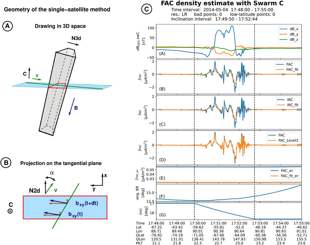
FIGURE 1. FAC density estimate by single-satellite method. (A): Schematic of a current sheet oriented along the local magnetic field B and normal direction along N3d sampled by a satellite moving with velocity v. (B): Schematic projection on the plane perpendicular to the local radial direction C. Here b designates the magnetic field perturbation. (C): Standard plot generated by the j1sat algorithm. From top to bottom the figure shows (A) the Swarm magnetic field perturbation in GEO frame, (B) the un-filtered and filtered FAC densities, (C) the un-filtered and filtered IRC densities, (D) a comparison between FAC estimated with j1sat and the Level-2 product, (E) the errors in un-filtered and filtered FAC densities, (F) the angle between the local magnetic field and the radial direction, and (G) the angle α in the tangential plane between the current sheet normal and the satellite velocity. The labels at the bottom presents time in UTC, the satellite geographic and quasi-dipole latitude and longitude, as well as the magnetic local time.

The FAC density j_FAC is simply obtained as

$j_{\text{FAC}}=\frac{j_{IRC}}{\cos \beta }(3)$

where β designates the inclination of magnetic field, i.e. the angle between C and B. Note that for Eq. 3 to be used in practice, one needs β values not too close to 90°, a condition always satisfied at auroral latitude but not near the equatorial region.

When no information on current sheet orientation is provided (the default running option), the algorithm assumes normal satellite incidence, i.e. N_2d along the satellite velocity vector v. Otherwise, this information can be supplied as the N_3d vector or, similarly, in the form of N_2d or α (the angle between N_2d and v). All the computations are performed in the GEO frame.

2.2 Dual-satellite FAC estimation

SwarmFACE provides three high-level function to estimate the FAC densities from dual-satellite measurements. All these algorithms follow a similar procedure that differs only in the last step, i.e. point (3) below:

1. Four-point configurations (quads) are formed along the orbit by combining two virtual positions from each satellite. To ensure, as much as possible, formation of regular quads, data from one satellite is time-shifted in the first place;

2. The magnetic field perturbations recorded by the two satellites are low-pass filtered, to minimize the influence of small-scale fluctuations at each satellite and to match the scale of the magnetic perturbations with the configuration scale;

3. The discretized form of the Ampère’s law is used to infer the current flowing through the quad and the FAC density is estimated by considering the orientation of local magnetic field.

Below we provide details and underline the characteristics of each algorithm available in SwarmFACE package. In this process we take as reference the algorithm used to generate the official Level-2 product (see Ritter et al., 2013).

2.2.1 Dual-satellite FAC estimation by Least Squares

The algorithm based on the Least Squares method, developed in Vogt et al. (2013), offers a series of advantages over the corresponding Level-2 FAC algorithm, listed below. For a detailed analysis on these aspects, the reader is referred to Blagau and Vogt (2019), illustrated with suggestive Swarm events.

Firstly, the method yields more stable solutions for “extreme” configurations, when the influence of local magnetic field perturbations is highly amplified (e.g. the very elongated quads near the orbital cross-points or the skewed quads encounter during the more recent Swarm phase, with closer orbital planes for the lower satellites). The explanation resides on the fact that one deals with an over-determined problem (i.e. observations from three, instead of four points in a plane are in principle enough to estimate the normal component of curl operator) and the LS approach accommodates the contributions of all points by minimizing the estimation errors. The more stable solution of the LS algorithm implies a reduction in the so-called Exclusion Zone (EZ), i.e. the regions near the cross-orbit points where the quad configurations becomes too elongated and the current density estimate is not provided due to its artificially high values.

Then, the configuration geometry considered in the algorithm is more general, see Figure 2A [reproduced from Vogt et al. (2013)]. As a result, deviations from parallel satellite orbits or skewed configurations are properly taken into account. This allows, in principle, to apply the algorithm not only to the pair of lower Swarm satellites but, occasionally, to combine data from Swarm B and Swarm A or Swarm C, provided that all three satellites form a close configuration.

FIGURE 2

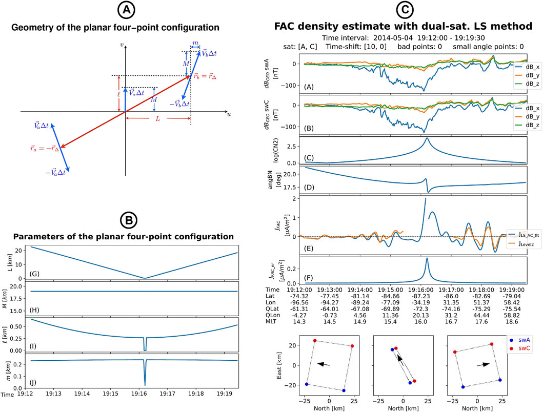
FIGURE 2. FAC density estimate by dual-satellite LS method. (A): Geometry of the planar four-point configuration in the dual-satellite methods. The different parameters that characterizes the configurations are L (half cross track separation), M (half along track separation), ℓ (half orbital lag) and m, with ϵ = m/M describing the deviation of satellite trajectories from parallel orbits. Taken from Vogt et al. (2013). (B): Parameters of the planar four-point configuration for the event shown on the right. The evolution along the orbit of L, M, ℓ, and m are presented in panels G–J. (C): Standard plot generated by the j2satLS algorithm. From top to bottom the figure shows (A and B) the Swarm magnetic field perturbation in the GEO frame, (C) the logarithm of the condition number, (D) the angle between B and the direction normal to the quad, (E) comparison between the dual-satellite LS FAC estimation (blue) and the Level-2 product (orange), and (F) the error level in FAC density estimation. At the bottom, the quad configuration at three instances (i.e. start time, stop time, and at the middle of the interval) is presented as projection on the North-East plane of the local NEC frame.

In addition, the method provides a robust way to infer the level of errors in FAC estimations as a function of quad geometry and magnetic field uncertainties. The error estimation scheme comes naturally from the formalism and has been endorsed by Monte-Carlo simulations.

Below, one reproduces a short description of the LS algorithm; for details the reader is referred to the original paper of Vogt et al. (2013). If f designates one component of the magnetic field perturbation in the plane of the quad (the (u, v) plane in Figure 2A), with $f_{\sigma }=f_{a,b}^{+,-}$ the values at the leading and trailing apex for satellite a and b, and with ${\mathit{r}}_{\sigma }={\mathit{r}}_{a,b}^{+,-}$ the corresponding position vectors, then the components of its planar gradient ∇_p f can be expressed as

${\nabla }_{p}f=\sum _{\sigma =1}^4{f}_{\sigma }{\mathit{q}}_{\sigma }=f_a^{+}{\mathit{q}}_a^{+}+f_a^{-}{\mathit{q}}_a^{-}+f_b^{+}{\mathit{q}}_b^{+}+f_b^{-}{\mathit{q}}_b^{-}(4)$

Here q_σ are the so called canonical base vectors; to find them, one has to solve the equations

${\mathbf{R}}_{\mathit{pos}}{\mathit{q}}_{\sigma }={\mathit{r}}_{\sigma },(5)$

where R_pos is the position tensor ${\mathbf{R}}_{\mathit{pos}}={\sum }_{\sigma =1}^4{\mathit{r}}_{\sigma }{\mathit{r}}_{\sigma }^t$, represented by a 2 × 2 matrix in the (u, v) coordinates. One critical aspect of the algorithm is related to this inversion problem. The stability of the solution to Eq. 5 is characterized by the so called condition number (a factor that enters in the error estimation scheme) CN = λ_max/λ_min, where λ_max and λ_min are the eigenvalues of R_pos arranged in descending order.

Assuming mutually uncorrelated and isotropic magnetic field errors at the points of measurements, i.e. $<\delta {\mathbf{b}}_{\sigma }\delta {\mathbf{b}}_{\tau }>={\delta }_{\sigma \tau }{(\delta b)}^2\mathbf{I}$, with σ, τ sensor indexes, δ_στ the Kronecker symbol, and I the unit matrix, then the mean square error of the radial current j_n through the spacecraft plane is provided by

$⟨|\delta j_n{|}^2⟩=\frac{{\left(\delta b\right)}^2}{{\mu }_0^2}\sum _{\sigma }|{\mathbf{q}}_{\sigma }{|}^2(6)$

Note that in Vogt et al. (2013) the symbol R is used for the position tensor. In this paper we adhere to the notations from Vogt et al. (2020), where R designates the position matrix and the position tensor is indicated by R_pos (see below).

2.2.2 Dual-satellite FAC estimation by Singular Value Decomposition

The dual-satellite SVD algorithm from SwarmFACE represents an adaptation of the more general RASADA (from Robust Adaptive Spacecraft Array Derivative Analysis) method and code developed in Vogt et al. (2020). RASADA allows to estimate the spatial derivative of physical quantities and their corresponding errors from an array of arbitrary numbers of satellites/observation points. Remarkably, the method automatically adapts to possible degenerate geometries of the array configuration, that could be a source of large estimation errors, by identifying and keeping only non-degenerate directions in the analysis.

The general RASADA algorithm is clearly described in Vogt et al. (2020), Section 2. Below we present the computation steps adapted to the context of Swarm dual-satellite FAC estimation:

1. The quad’s position vectors r_σ, computed with respect to the quad center (i.e. in the mesocentric frame, where ${\sum }_{\sigma =1}^4{\mathbf{r}}_{\sigma }=0$) are stored as rows in the (4 × 3) position matrix R. The position matrix R is related to the position tensor ${\mathbf{R}}_{\mathit{pos}}={\sum }_{\sigma =1}^4{\mathit{r}}_{\sigma }{\mathit{r}}_{\sigma }^t$ by R_pos = R^tR.

2. The SVD of the position matrix is performed, R = USV^t, where U is a (4 × 3) matrix satisfying UU^t = I (with I the unit matrix) and V is a (3 × 3) orthogonal matrix satisfying VV^t = V^tV = I. The (3 × 3) matrix S is diagonal; since in our case the configuration is degenerated to a planar geometry, S has only two non-zero elements, S = diag(R⁽¹⁾, R⁽²⁾, 0). Here R⁽¹⁾ ≥ R⁽²⁾ ≥ 0.

3. Form a stable pseudoinverse of S. For that purpose, compute τ = R⁽²⁾/R⁽¹⁾; if τ is below a set threshold τ₀, meaning that the quad’s configuration is too elongated along the direction associated with R⁽¹⁾ (i.e. close to linear degeneracy), consider only the first eigenvalue during the inversion:

${\mathbf{S}}^{-}=\left\{\begin{array}{ccc}\text{diag}\left(1/R^{\left(1\right)},1/R^{\left(2\right)},0\right)\hfill & \hfill \mathrm{i}\mathrm{f}\hfill & \tau \ge {\tau }_0\hfill \\ \text{diag}\left(1/R^{\left(1\right)},\mathrm{0,0}\right)\hfill & \hfill \mathrm{i}\mathrm{f}\hfill & \tau <{\tau }_0\hfill \end{array}\right.(7)$

4. Compute the (4 × 3) matrix Q = US⁻V^t. The rows of Q are the (generalized) reciprocal vectors q_σ, σ = 1, … 4

5. Considering the magnetic field perturbation at the quad’s vertices b_σ, σ = 1, … 4, the curl c = ∇ ×b is estimated through c ≃∑_σq_σ ×b_σ

6. Assuming isotropic and mutually uncorrelated instrumental errors δb for each component of b, the mean square error of the radial current j_n through the spacecraft plane is provided by $⟨|\delta j_n{|}^2⟩=\mathrm{t}\mathrm{r}\mathrm{a}\mathrm{c}\mathrm{e}({\mathbf{Q}}^t\mathbf{Q}){(\delta b)}^2/{\mu }_0^2$

According to third step above, when τ ≥ τ₀ the quad configuration is considered non-degenerated (to a linear geometry) and the LS and SVD provides exactly the same solution. Near the orbital cross-points, when τ < τ₀, only the eigenvector associated with the biggest eigenvalue (i.e. the along-track direction) is used in the analysis and the algorithm yields estimates that are close to the average (over the satellites) single-satellite estimates. This provides the notable advantage to have dual-satellite based FAC solutions with no data gaps in the region close to the orbital cross-points.

Nevertheless, the transitions between different gradient estimator at the point where the singular ratio threshold τ₀ is crossed leads to discontinuous current density solutions. In the SwarmFACE implementation of the SVD algorithm, when such discontinuous behavior is undesired, the transitions may be smoothed by using a pseudoinverse matrix of the form S⁻ = diag(1/R⁽¹⁾, f(τ)/R⁽²⁾, 0), with the function f = f(τ) defined in a stepwise manner:

$f\left(\tau \right)=\left\{\begin{array}{ccc}1\hfill & \hfill \mathrm{i}\mathrm{f}\hfill & \tau \ge \tau *,\hfill \\ g\left(\tau \right)\hfill & \hfill \mathrm{i}\mathrm{f}\hfill & \tau *>\tau \ge {\tau }_0,\hfill \\ 0\hfill & \hfill \mathrm{i}\mathrm{f}\hfill & {\tau }_0>\tau .\hfill \end{array}\right.(8)$

A second threshold parameter, i.e. τ* ≥ τ₀, is thus introduced. The function g = g(τ) allows for continuous connection between the first (τ ≥ τ*) and third (τ < τ₀) branches of f. Two options are implemented for g, i.e. the linear interpolation

$g_{\text{lin}}\left(\tau \right)=\frac{\tau -{\tau }_0}{\tau *-{\tau }_0}(9)$

and cubic (spline) interpolation, which allows for smooth (differentiable) continuation

$g_{\text{cub}}\left(\tau \right)=\left(3-2\frac{\tau -{\tau }_0}{\tau *-{\tau }_0}\right){\left(\frac{\tau -{\tau }_0}{\tau *-{\tau }_0}\right)}^2.(10)$

Note that the original behavior (no interpolation) is recovered with τ* = τ₀.

As in the case of the LS algorithm, the method provides a robust framework for error assessment, based on the local quantities (e.g. array configuration and magnetic field measurement uncertainties), as indicated in the sixth step above. This is valid also for the region with τ < τ₀, where the SVD algorithm predicts the same error level as in the case of the single-satellite method (Eq. (2)) with a sampling distance L given by the along-track separation.

Besides the error assessment, two additional parameters are useful to monitor the SVD solution. One is the condition number, used also in the LS algorithm to characterize the solution stability, i.e. CN = λ_max/λ_min, where λ_max and λ_min are the eigenvalues of the position tensor R_pos. In the SVD case one recovers the same parameter by using CN = 1/τ². A second parameter indicates the configuration/array degeneracy AD, which in the standard RASADA dual-satellite algorithm has two values, i.e. AD = 2 for τ ≥ τ₀ and AD = 1 otherwise. In SwarmFACE implementation of SVD algorithm one uses AD = 1 + f(τ), with f(τ) provided in Eq. (8).

2.2.3 Dual-satellite FAC estimation by Boundary Integral

The Level-2 FAC product is based on the BI approach to FAC estimation introduced by Ritter and Lühr (2006) and further elaborated in Ritter et al. (2013). Alternatively, Shen et al. (2012) introduced the Finite Differencing (FD) method to estimate the full magnetic field gradient with a Swarm-like mission. The equivalence of FD and BI curl estimation techniques using planar four-point configurations has been demonstrated in Vogt et al. (2013) where the estimators are also brought to a canonical form (see Section 3.3 in that paper), suitable to be used in an error estimation scheme.

SwarmFACE package provides one function based on BI approach that differs in two important aspects from the Level-2 algorithm: (i) equations based on rectangular (instead of spherical) geometry are used, which adds considerable stability to the solutions (i.e. a significant reduction of the EZ) and (ii) the error analysis is based on the canonical base vectors formalism, that has been endorsed by Monte-Carlo simulations (Blagau and Vogt, 2019).

We reproduce from Vogt et al. (2013) the important equations used in the algorithm. The contour integral over the sides of the quad shown in Figure 2A can be evaluated with the trapezoidal rule yielding (after some arrangements):

$\oint \mathbf{b}\cdot d\mathbf{s}\approx \frac{1}{2}\left[\left({\mathbf{b}}_b^{+}-{\mathbf{b}}_a^{-}\right)\cdot \left({\mathbf{r}}_a^{+}-{\mathbf{r}}_b^{-}\right)-\left({\mathbf{b}}_a^{+}-{\mathbf{b}}_b^{-}\right)\cdot \left({\mathbf{r}}_b^{+}-{\mathbf{r}}_a^{-}\right)\right](11)$

while the area of the quad is

$A=\frac{1}{2}\left({\mathbf{r}}_a^{-}-{\mathbf{r}}_a^{+}\right)\cdot \left({\mathbf{r}}_b^{+}-{\mathbf{r}}_a^{+}\right)+\frac{1}{2}\left({\mathbf{r}}_b^{+}-{\mathbf{r}}_b^{-}\right)\cdot \left({\mathbf{r}}_a^{-}-{\mathbf{r}}_b^{-}\right)(12)$

which leads to the current density estimation along the normal direction

$j_n=\frac{1}{{\mu }_{0}A}\oint \mathbf{b}\cdot d\mathbf{s}(13)$

The mean square error of the radial current j_n through the spacecraft plane is provided by

$⟨|\delta j_n{|}^2⟩=\frac{{\left(\delta b\right)}^2}{{\mu }_0^2}\frac{1}{4L^2{\mu }^2}\left(1+{\mu }^2+{\lambda }^2\right)(14)$

The significance of parameters L, μ, and λ is closely related to the configuration shown in Figure 2A: (i) the quantity 2L is the spatial separation between the satellite orbits, (ii) if one designates by 2ℓ the satellites’ separation in orbital phase, then λ = ℓ/L measures the configuration skewness (deviation from an equal-sided trapezoid), (iii) if 2M describes the along track separation, then μ = M/L measures the quad elongation, i.e. the along-track separation relative to the cross-track distance. The parameter m in Figure 2A [not entering in Eq. (14)] indicates the deviation from parallelism of the satellite tracks.

Eq. (6), providing the mean square error of the radial current in the LS method, can also be expressed as a function of configuration parameters using only a slightly more complicated form than Eq. (14) (Vogt et al., 2013). However, there we used an expression that involves the canonical base vectors q_σ, obtained directly from the inversion problem in Eq. (5). Contrary to that, in the case of the BI approach, one has to compute the configuration parameters in every point where the FAC density is estimated.

2.3 Three-satellite FAC estimation

Since the upper and the lower Swarm satellites have different orbital velocities, they are periodically aligned in latitude in the auroral zone. When, in addition, a close constellation is formed, the FAC density can be estimated by applying the three-s/c method developed in Vogt et al. (2009). The latter condition is important since the orbital plane of Swarm B has a relative drift (of ∼ 22.5°/year) with respect of the orbital planes of the lower satellites that could lead to a configuration too stretched in longitude when compared with the longitudinal characteristic scale of the FAC sheets. Suitable events are therefore expected at the beginning of the mission (orbital planes roughly aligned), during the more recent Swarm phase when Swarm B and Swarm A/C are orbiting the Earth in opposite directions (orbital planes of ∼ 180° at the beginning of October 2021) or, occasionally, at very high latitude. SwarmFACE provides a tool to find Swarm conjunctions above the auroral oval, see Sections 3.4.

When applicable, the three-satellite method provides the unique opportunity of estimating the FAC density at a different scale, larger than in the dual-satellite case. In addition, since the method does not assume time-stationary current structures (unless the user prefers to time-shift the data, e.g. to obtain a more favorable geometry), one can in principle use data with higher temporal resolution as input. For a more detailed discussion of the three-satellite method in the context of Swarm, the reader is referred to Blagau and Vogt (2019).

Below, the recipe for inferring the current density along the direction normal to the spacecraft plane is provided [from Vogt et al. (2009)]. If r_α, α = 1, 2, 3 are the satellite’s position vectors in the mesocentric frame (the frame where ${\sum }_{\alpha =1}^3{\mathit{r}}_{\alpha }=0$), and r_αβ = r_β−r_α are the relative position vectors, the planar reciprocal vectors q_α are formed as

${\mathit{q}}_{\alpha }=\frac{\mathit{n}\times {\mathit{r}}_{\beta \gamma }}{|\mathit{n}{|}^2},\alpha =\mathrm{1,2,3}(15)$

where (α, β, γ) are cyclic permutations of (1, 2, 3), and n is the vector normal to the spacecraft plane defined as n = r₁₂ ×r₁₃. The curl of magnetic field perturbations along the normal direction is then provided by

${\left(\nabla \times \mathit{b}\right)}_n\approx \left(\sum _{\alpha =1}^3{\mathit{q}}_{\alpha }\times {\mathit{b}}_{\alpha }\right)\cdot \mathit{n}(16)$

with b_α being the magnetic field perturbation recorded by satellite α. With similar assumptions as in the case of dual-satellite LS method, Eq. (6) can be used to estimate the mean square error of the current density along the normal direction. Alternatively, the quality of the planar gradient estimate can be assessed from the position tensor ${\mathbf{R}}_{\mathit{pos}}={\sum }_{\alpha =1}^3{\mathit{r}}_{\alpha }{\mathit{r}}_{\alpha }^t$ (represented by a singular matrix in this case) through the so-called condition number, i.e. the ratio of its (non-zero) eigenvalues.

2.4 Minimum Variance Analysis and correlation analysis on Swarm data

For judging the quality of current density estimations it is important to evaluate to what degree the sampled current structure satisfies the assumptions on which the FAC method(s) rely. For example, the standard single-satellite FAC algorithm assumes one-dimensional/planar magnetic field structure and normal satellite incidence. A certain degree of time stationarity is required in the dual-s/c algorithm as well as in the three-s/c method when virtual (i.e. not instantaneous) satellite positions are employed. SwarmFACE provides functions that automatically estimate the so-called quality indices, like current sheet planarity, inclination and correlation of magnetic perturbations recorded by the lower satellite.

One way to assess the degree of planarity and the inclination of a current structure is by applying the MVA analysis, introduced in (Sonnerup and Cahill, 1967). A short description of the algorithm used in the SwarmFACE package is provided below; for an extensive derivation the reader is referred to Sonnerup and Scheible (1998) and Sonnerup et al. (2006).

Given the magnetic field perturbation recorded during the current sheet crossing, b^(k), k = 1, 2 … K, the standard version of MVA searches for the direction n that minimizes the quantity (magnetic field variance)

${\sigma }^2=\frac{1}{K}\sum _{k=1}^K{\left|\left({\mathbf{b}}^{\left(k\right)}-⟨\mathbf{b}⟩\right)\cdot \mathbf{n}\right|}^2(17)$

subject to the condition that |n|² = 1, and associates it with the current sheet normal. Here by $⟨\cdots ⟩$ the mean over the set of K points of measurements is indicated. The minimization leads to an eigenvalue problem for the (symmetric) 3 × 3 magnetic variance matrix M^B, defined as

${\mathbf{M}}^B=⟨\left(\mathbf{b}-\langle \mathbf{b}\rangle \right){\left(\mathbf{b}-\langle \mathbf{b}\rangle \right)}^t⟩=⟨\mathbf{b}{\mathbf{b}}^t⟩-\langle \mathbf{b}\rangle \langle {\mathbf{b}\rangle }^t(18)$

with the eigenvector corresponding to the smallest eigenvalue of M^B providing the n direction. In case of a FAC structure the magnetic perturbations roughly occur only perpendicular to the ambient magnetic field B. That can be taken into account if one replaces the matrix M^B by the matrix product PM^BP, where p represents the so-called projection matrix, given by

$\mathbf{P}=\mathbf{I}-\mathbf{m}{\mathbf{m}}^t(19)$

with $\mathbf{m}=⟨\mathbf{B}⟩/\left|⟨\mathbf{B}⟩\right|$. This way of performing the analysis, implemented in SwarmFACE, is know as the constrained (to average ambient magnetic field direction) MVA.

The vector n identified by MVA corresponds to N_3d indicated in Figure 1A, from which the vector N_2d and the inclination angle α in the tangential plane can be obtained. A measure of the current sheet planarity is provided by the ratio λ_max/λ_min, with λ_max and λ_min the two eigenvalues of the (constrained) magnetic variance matrix.

For case studies, SwarmFACE allows the user to interactively select the analysis interval that enters MVA (see Section 3.5). To automatically estimate the planarity and inclination for a number of consecutive orbits (see Section 3.6), SwarmFACE performs MVA on the auroral oval (AO) intervals estimated with the lower-level function find_ao_margins. This function works on quarter-orbit sectors and therefore in the automatic procedure the initial data interval is first split in sections using as delimiters the moments when the satellite is either above the Equator or when the highest/lowest quasi-dipole magnetic latitude (QDLat) is reached. Note that for each such sector the evolution of QDLat is monotonic.

The following steps are pursued by find_ao_margins to find the AO location on a quarter-orbit sector:

1. The single-satellite FAC density estimate is considered and the cumulative sum (integral) of unsigned (absolute value) FAC density is computed. The integration is performed as a function of QDLat (not time), to correct for the non-linear changes in QDLat at the highest/lowest portion of the orbit. Since in the process of current integration, small FAC densities could badly affect the good identification of auroral oval, only current densities above a certain value are considered;

2. The points d₁, d₂, and d₃ when the integral reaches a fraction of 1/4, 1/2, and 3/4 from its total height are identified;

3. The timestamps corresponding to d₁−(d₃−d₁), d₂, and d₃+(d₃−d₁) are associated with the beginning, the center, and the end of the AO interval. If the beginning/end timestamp falls outside the quarter-orbit section, its beginning/end time is used.

A hint on the current-sheet time-stationarity or its compliance to the one dimensional model (the two aspects are difficult to dis-entangle) could be obtained with the correlation analysis. SwarmFACE provides a function that estimates the correlation of magnetic field perturbations recorded by the lower Swarm satellites. To that end.

1. The MVA analysis is performed on Swarm A and Swarm C data and the magnetic perturbations along the maximum variance directions are further used;

2. Data from the satellite with the shorter MVA interval, trimmed to this interval, form the reference signal;

3. A running Pearson’s correlation coefficient is computed by comparing the time-shifted versions of the reference signal (typically in the ± 30 s range) with data intervals of the same length from the other satellite;

4. The highest correlation coefficient is returned, together with the identified optimum time-lag.

3 Code usage and results

3.1 Single satellite FAC estimation

To estimate the FAC density with one satellite, SwarmFACE provides the j1sat high-level routine:

Listing 1. The full calling sequence for j1sat high-level routine

The mandatory parameters specify the analysis interval start and end time (parameters dtime_beg and dtime_end), and the Swarm satellite sat. With only these parameters provided, the program computes the low-resolution FAC density assuming normal current sheet orientation.

The actual current orientation should be inferred separately, e.g. by applying MVA on the auroral oval interval (see Section 2.4 and Section 3.5), and can be passed to j1sat by one of the N3d, N2d, or alpha parameters. Here N3d and N2d designate (in geographic frame) the full current sheet normal vector and, respectively, its projection on the tangential plane, while alpha refer to the angle α between the N_2d and the satellite velocity, see Figure 1B. Internally, when α is not provided by outside, the algorithm uses N_3d or N_2d to compute its values along the orbit and further work with these in the calculations. Note that, since the standard MVA provides the constant vector N_3d (assumed to characterize globally the auroral crossing), α is (moderately) varying in time and therefore the user can provide alpha either as an average value or as an array of successive values. The parameter tincl allows to specify the time interval when the information on current sheet inclination is valid, typically the interval used in MVA. When not specified, the whole analysis interval, i.e. [dtime_beg, dtime_end] is considered valid, which could lead to undesired results since, e.g. the angle between N_3d and satellite velocity v could then vary substantially. When tincl is provided, the algorithm will use the first/last value of α to calculate the inclination before/after its margins.

With the parameter use_filter, the users specify whether or not they want to pre-filter the input magnetic field perturbations that enters the FAC estimation, its default value being True (i.e. to use the filter). The parameters er_db and angTHR specify the level of uncertainties in magnetic field measurements (considered in the current density error calculation) and, respectively, the minimum accepted angle of the magnetic field vector from the tangential plane, needed to estimate FAC from IRC density with Eq. (3). The last two parameters, i. e savedata and saveplot, are for saving the results as an ASCII file and, respectively, in a plotted format.

The first two objects from the j1sat output are pandas DataFrame structures. j_df contain all relevant results, i.e. satellite position at the times of FAC estimations, the un-filtered and (if requested so) filtered FAC and IRC densities together with the corresponding errors, the angle between B and C and the α angle. Similarly, input_df essentially contains the input data, as retrieved from ESA database, like satellite position in GEO frame, the magnetic field measurements and the model data in NEC frame. param is a dictionary object with all the parameters used in the analysis. It also contains a field for missing or bad Swarm measurements.

Figure 1C presents the standard plot generated by j1sat when saveplot = True. After the MVA has been applied for this event, the FAC normal N3d = [0.227, 0.692, 0.684], valid for the time indicated by dashed vertical lines, has been supplied to j1sat. From top to bottom, the figure shows (A) the Swarm magnetic field perturbation in GEO frame, (B) the un-filtered and filtered FAC densities, (C) the un-filtered and filtered IRC densities, (D) a comparison between FAC estimated with j1sat and the Level-2 product, (E) the errors in un-filtered and filtered FAC densities, (F) the angle between B and C vectors, and (G) the α angle. The labels at the bottom indicate time in UTC, the satellite geographic and quasi-dipole latitude and longitude, as well as the magnetic local time.

3.2 Dual-satellite FAC estimation

The SwarmFACE dual-satellite routines implicitly run on the same configurations as the official Level-2 algorithm, i.e. the sensors are (as much as possible) aligned in orbital phase and a 5 s travel distance for the along track separation is chosen to construct the quads. However, the user can take advantage of the flexible geometry shown in Figure 2A and work e.g. with smaller along-track separation distance to investigate FAC structures at higher spatial resolution or the orbital time lag between the satellites such that the quad configuration is tuned to better characterize current sheets inclined with respect to spacecraft orbit (see Section 3.4 in Blagau and Vogt, 2019). To reduce the influence of local magnetic fluctuations, the magnetic perturbation is pre-filtered with a 20 s cut-off low-pass Butterworth filter (see also the discussion at the beginning of Section 2).

3.2.1 Dual-satellite FAC estimation by Least Squares

The dual-satellite LS algorithm is implemented with the j2satLS high-level routine:

Listing 2. The full calling sequence for j2satLS high-level routine

Here sats is a 2 element array of strings that designates the satellites entering in the analysis, usually the lower Swarm pair, i.e. sats = [′A′, ′C′]. The parameters dt_along and tshift specify the quad’s length in the along-track direction (in seconds of satellite travel distance) and, respectively, the time shift (in seconds) to be introduced in satellite data in order to achieve the desired quad configuration. When tshift (a 2 element array of integer numbers) is not specified, the program uses the lower level find_tshift2sat routine to find the optimal time-shift that ensures formation of rectangular quads. Since find_tshift2sat firstly estimates the orientation of orbital planes from the downloaded satellite positions, it is advisable to avoid using small intervals of analysis. For the nominal separation of 1.4^◦ between the orbital planes of Swarm lower satellites, an interval of analysis of at least 2 min provides good estimates; however, this could be insufficient during the close orbit configuration campaign centered around October 2021. Note that in the standard plots generated by j2satLS, the quad configurations are plotted at the bottom, so that the user can judge whether or not the parameter tshift has been correctly computed.

For a regular analysis the parameter use_filter should be left unchanged to its implicit value, i.e. True, meaning to pre-filter the magnetic field perturbation. For a discussion on working with un-filtered data in dual-satellite FAC method, the reader is referred to Blagau and Vogt (2019), Section 3.4.2. The parameter errTHR specifies the accepted error estimation level for the IRC density, the prime quantity evaluated by the algorithm, see Eq. (6); whenever j_n is below this threshold, IRC and FAC densities are set to NaN.

When knowing the parameters that describe the planar four-point configuration is desired, the users could set saveconf = True, which will add new columns in the j_df DataFrame. These parameters, shown in Figure 2A and introduced in Section 2.2.3, need not to be computed in the LS method [though, they are used to estimate the errors in the BI method, see Eq. (14)]. Nevertheless, the evolution of quad parameters along the orbit could be instructive, as shown in Figure 2B, which refers to the event presented in Figure 2C. The first two panels, (G) and (H), indicate how the (half) cross-track separation L acquires a minimum value at the orbital cross-point, while the (half) along-track separation M is constant. The other two parameters, i.e. ℓ and m, that describe the (un-compensated) orbital lag and the non-parallelism of the satellite tracks, are shown in panels (I) and, respectively, (J). Their values drop around the orbital cross-point because the algorithm takes care of assigning to each vertex the correct satellite positions in order to maintain a convex configuration (as needed in the BI method).

The output from j2satLS is structured in a way similar to the j1sat output: j_df and input_df are pandas DataFrames that hold the result and the input data, respectively, while param is a dictionary with all the parameters used in the analysis, including a field for missing or bad Swarm measurements.

Figure 2C presents the standard plot generated by j2satLS when saveplot = True. From top to bottom the figure shows (A, B) the Swarm magnetic field perturbation recorded by the two satellites in GEO frame, (C) the logarithm of the condition number, as defined in Section 2.2.1, (D) the angle between the local magnetic vector and the direction normal to the quad, (E) comparison between the dual-satellite LS FAC estimation (blue) and the Level-2 product (orange), and (F) the error level in FAC density estimation. At the bottom, the quad configuration at three instances (i.e. start time, stop time, and at the middle of the interval) is presented as projection on the North-East plane of the local NEC frame. Note in panel (E) the different EZ extensions for the Level-2 solution [±4° co-latitude, according to Ritter et al. (2013)] and in the LS solution, set by the value specified in errTHR (here we chose a level of 0.25 μA/m² for errTHR, to make evident the differences with respect to the BI algorithm, see Section 3.2.3).

3.2.2 Dual-satellite FAC estimation by Singular Value Decomposition

The dual-satellite SVD algorithm is implemented with the j2satSVD high-level routine:

Listing 3. The full calling sequence for j2satSVD high-level routine

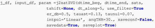
Here the characteristic parameters are tauast, taunul, and intpol; the first two specify the threshold values τ* and τ₀, whereas the last one indicates the interpolation method to be used for matching the different gradient estimators, i.e. the branches for τ ≥ τ_* and τ < τ₀, respectively (see Section 2.2.2). Values for intpol should be ‘Linear’ (for linear interpolation; the default value), ‘Cubic’ (for cubic spline interpolation), or None (when no interpolation is desired; in this case the tauast parameter is ignored and the standard RASADA algorithm is applied with the threshold value specified by taunul).

Figure 3A presents the standard plot generated by j2satSVD when saveplot = True. Comparing with the standard plot produced by the LS routine, an additional panel (the new panel E) has been introduced that presents the evolution of two parameters, i.e. τ (matrix S eigenvalues ratio) and the array degeneracy AD, as defined in Section 2.2.2. Far enough from the orbital cross-point AD = 2 and the SVD and LS solution are identical. When τ is below the threshold set by taunul, AD = 1 and the SVD algorithm provides a solution close to the average (over the satellites) single-satellite estimates. In that region also the magnetic field angle (panel D) is calculated with respect to the radial direction (not with respect to the quad normal).

FIGURE 3

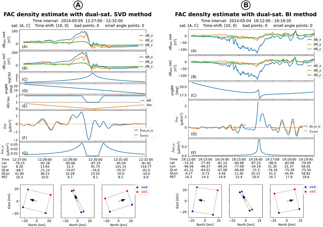
FIGURE 3. (A): Standard plot generated by the j2satSVD algorithm. The figure is similar to Figure 2C, with an additional panel (the new panel E) that presents the evolution of eigenvalue ratio τ (orange line) and the array degeneracy AD (blue line). (B): Standard plot generated by the j2satBI algorithm. The same quantities as in Figure 2C are plotted, with the exception of the condition number, which is not computed by the algorithm.

The error in FAC estimation (panel G) are increasing as τ decreases toward the τ* level. For even smaller values of τ, the error starts to decrease up to the level predicted by the single-satellite method for a sampling distance given by the along-track separation (region where τ < τ₀). As one can see, the implicit values used in the SVD algorithm (0.13 for tauast and 0.07 for taunul) provide a more conservative current density estimate than in the LS case, since the error level remains below 0.05 μA/m², i.e. the implicitly accepted threshold used to control the LS solution (see the parameter errTHR from Section 3.2.1).

3.2.3 Dual-satellite FAC estimation by Boundary Integral

The dual-satellite BI algorithm, implemented with the j2satBI high-level routine, requires the same parameters as in the LS case:

Listing 4. The full calling sequence for j2satBI high-level routine

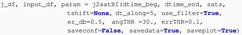
Figure 3B presents the standard plot generated by j2satBI for the same event analyzed with the LS algorithm (see Figure 2C). Only five panels are needed since no condition number is computed. We used the same threshold value for errTHR to put in evidence higher values/lower stability for the BI FAC estimate close to the orbital cross-point (compare panel E in Figure 2C with panel D in Figure 3B) as well as broader evolution of FAC errors in that region (last panels in the same plots). When compared with the Level-2 product (panel D in Figure 3B), the j2satBI solution shows greater stability, although it relies on the same, i.e. BI, method the only difference being that j2satBI uses equations based on rectangular (instead of spherical) geometry.

3.3 Three-satellite FAC estimation

The three-satellite algorithm, intended to be applied when the Swarm satellites form a close configuration, is implemented with the j3sat high-level routine:

Listing 5. The full calling sequence for j3sat high-level routine

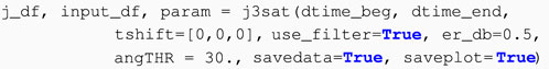
A parameter that specifies the satellite (like sats in the single- and dual-satellite routines) is not needed in this case. However, if the user decides to perform the analysis with shifted satellite position (e.g. to achieve a more favorable spacecraft constellation), the tshift parameter (now a three element array of integer numbers) should specify the time shifts in seconds keeping the internal order of satellites, i.e. Swarm A, Swarm B, and Swarm C.

Figure 4A presents the standard plot generated by j3sat when saveplot = True. From top to bottom, the figure shows (A–C) the Swarm magnetic field perturbation recorded by the Swarm satellites in GEO frame, (D) the logarithm of the condition number, as defined in Section 2.3, (E) the angle between the local magnetic field vector B and the direction normal to the spacecraft plane, (F) comparison between the un-filtered and (if use_filter = True) filtered three-satellite FAC estimations (blue and orange, respectively) and the Level-2 dual-satellite product (green), and (G) the error level in FAC density estimation(s). At the bottom, the spacecraft configuration at three instances (i.e. start time, stop time, and at the middle of the interval) is presented as projection on the North-East plane of the local NEC frame.

FIGURE 4

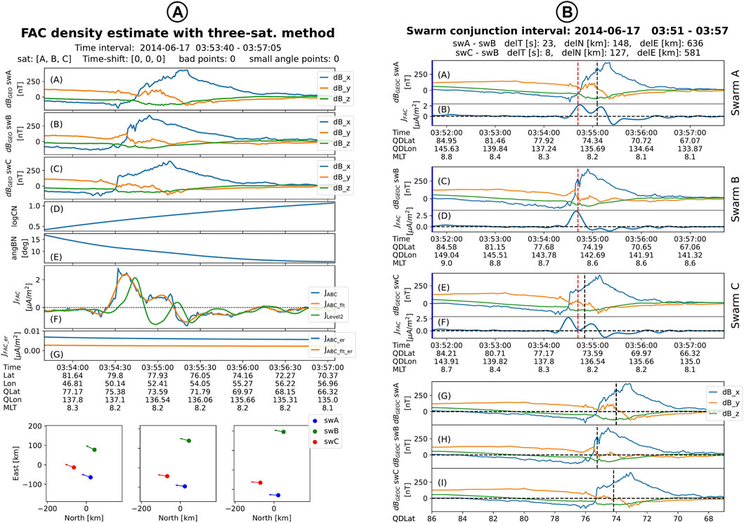
FIGURE 4. (A): Standard plot generated by the j3sat algorithm. From top to bottom the figure shows (A–C) the magnetic field perturbation recorded by the Swarm satellites in GEO frame, (D) the logarithm of the condition number, (E) the angle between B and the direction normal to the spacecraft plane, (F) comparison between the un-filtered and filtered three-satellite FAC estimations (blue and orange, respectively) and the Level-2 dual-satellite product (green), and (G) the error level in FAC density estimation(s). At the bottom, the spacecraft configuration at start time, stop time, and at the middle of the interval is presented as projection on the North-East plane of the local NEC frame. (B): Standard plot generated by the find_3sat_conj algorithm. The magnetic field perturbation in GEO panels (A, C, and E) and the low-pass filtered single-satellite Level-2 FAC density data (panels (B, D, and F) are plotted for each satellite. The panels (G, H, and I) present the magnetic field perturbation as a function of QDLat. The auroral central times/location are shown as vertical black dotted lines. In panels (A–F) the auroral central time for Swarm B is indicated as reference (the red doted lines).

To interpret the differences between dual- and three-satellite solutions (panel F), one should keep in mind that (i) these estimations refer to different points, i.e. the corresponding mesocenters have different latitude and longitude and (ii) the scales involved are different. A detailed discussion about the differences between dual- and three-satellite FAC estimations on the event presented in Figure 4A has been provided in Section 4.2 of Blagau and Vogt (2019). In the same paper, other critical aspects related to the application of three-sat method in the Swarm context (longitudinal separation, linear field variation, orientation of the spacecraft plane etc) are discussed.

3.4 Identification of Swarm conjunctions above the auroral oval

SwarmFACE package provides a tool to find Swarm conjunctions above the auroral oval. These events would then qualify to investigate the FAC structure with the three-satellite method or with the dual-satellite method when Swarm B data are combined with data from one lower Swarm satellite. The algorithm is implemented with the find_3sat_conj high-level routine:

Listing 6. The full calling sequence for find_3sat_conj high-level routine

The routine relies on the lower-level function find_ao_margins (see its description in Section 2.4) that automatically identifies the auroral oval location for each satellite. The following processing steps are performed:

1. For each satellite, the single-sat Level-2 FAC data corresponding to the full consecutive orbits that completely cover the time-interval provided by the user (i.e. a larger interval than [dtime_beg, dtime_end]) is downloaded with viresclient. In order to work with smaller arrays, only orbital sections where the quasi-dipole latitude is $>45°$ or $<-45°$ are retrieved. The FAC data are also filtered using a low-pass Butterworth filter

2. Data are split in quarter-orbits, as described in Section 2.4, and for each section find_ao_margins is called to estimate the central position of the auroral oval

3. Conjunctions are found by imposing temporal and spatial conditions, i.e. that Swarm B and Swarm A/C auroral oval central points to be encountered within a certain time-window (specified, in seconds, with the parameter delT), and within a certain spatial range along the North-South and East-West direction (specified, in km, with the parameter delN and, respectively, delE). The parameter jTHR (value in μA/m²) is used by find_ao_margins as a threshold to neglect small FAC densities that could badly affect the good identification of auroral oval (see Section 2.4)

The output from find_3sat_conj are the conj_df DataFrame object, with details on the identified conjunctions (e.g. conjunction time and location, time difference between the AO central times, spatial difference between the AO central locations), and param, a dictionary object of parameters used in the computation. The content of conj_df is always saved in an ASCII file. Since the automatic identification of AO intervals might not work accurately in all cases, it is advisable for the user to let the program generate standard plots, designed to help in (visually) assessing the quality of each conjunction (i.e. keep saveplot = True). Nevertheless, the generation of plots could be time consuming, mainly because the magnetic field data have to retrieved for each conjunction (5 min Before/after the central AO detected by Swarm B).

In Figure 4B one standard plot generated by find_3sat_conj is presented. The magnetic field perturbation in GEO (panels A, C, and E) and the low-pass filtered single-satellite Level-2 FAC density data (panels B, D, and F) are plotted for each satellite. The last three panels (i.e. G, H, and I) present the magnetic field perturbation as a function of QDLat. The auroral central times/locations are shown as vertical black dotted lines. In panels A–F the auroral central time for Swarm B is indicated as reference (the red doted lines). The plot subtitle provides details about the conjunction, e.g. the time and spatial difference between the central AO encountered by the satellites.

3.5 Interactive Minimum Variance Analysis on Swarm events

Besides the MVA on automatically identified AO intervals, SwarmFACE provides the user with the possibility to interactively select the interval for MVA on individual events. The necessary lines of code, to be run from a 2-cell jupyter notebook are presented below; the code could be adapted to other environments provided that an interactive backend for matplotlib is available. The first cell specifies the input parameters and prepares the necessary data for analysis.

Listing 7. First part of interactive Minimum Variance Analysis

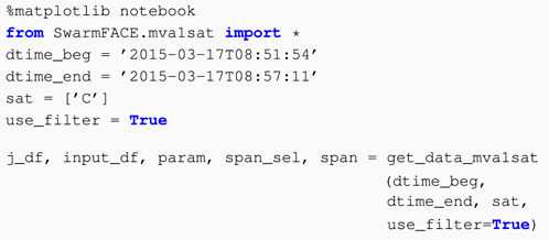
Note the %matplotlib notebook magic command at the beginning, that ensures the production of interactive plot(s) embedded within the notebook. The get_data_mva1sat routine retrieves (through viresclient) the 1 Hz resolution magnetic field data, computes the standard (i.e. assuming normal FAC inclination) single-satellite FAC density estimation and produces a plot of these variables on the output cell. The parameters dtime_beg and dtime_end can be only roughly specified; the algorithm actually downloads Swarm measurements on a larger interval, i.e. half-orbit time span, and offers the possibility to pan/zoom on the plotted data. If the users want to change the initial time-interval, i.e. [dtime_beg, dtime_end], they can do so by mouse clicking and adjusting, while vertical lines will indicate the new interval of analysis. This is achieved by calling (in the background) the matplotlib SpanSelector widget. The output variable span_sel holds the new interval of analysis, while span is a reference to SpanSelector that prevents it to be garbage collected, making it thus available outside get_data_mva1sat.

The second cell performs the MVA on the (up-dated, if necessary) analysis interval:

Listing 8. The second part of interactive Minimum Variance Analysis

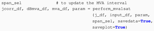
The perform_mva1sat routine takes as input the variables produced by get_data_mva1sat, i.e. j_df and input_df which are DataFrames that hold FAC density data and, respectively, the data retrieved from the ESA database. The output variables jcorr_df, dBmva_df, and mva_df are DataFrames with the corrected (for current sheet inclination) FAC density, magnetic field perturbation in MVA frame (the frame aligned along the MVA eigenvectors’ directions), and the result from the MVA analysis, respectively.

Figure 5A presents the plot generated by perform_mva1sat when saveplot = True. From top to bottom one has (A) the magnetic field perturbation in GEO, (B) the magnetic field perturbation in the MVA frame, (C) a comparison between the standard and corrected for inclination FAC density estimates, and (D) the angle in the tangential plane between the FAC sheet normal and the satellite velocity vector (angle α in Figure 1B). The hodograph of magnetic field perturbation in the plane perpendicular to the average magnetic field direction is presented in panel E.

FIGURE 5

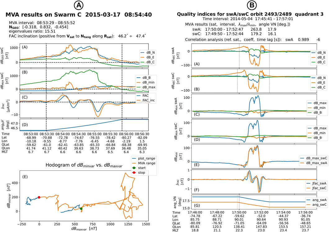
FIGURE 5. (A): Standard plot generated by perform_mva1sat. From top to bottom the figure shows (A and B) the magnetic field perturbation in GEO frame and MVA frame, respectively, (C) a comparison between the standard and corrected for inclination FAC density estimates, and (D) the angle in the tangential plane between the FAC sheet normal and the satellite velocity vector (angle α in Figure 1B). The hodograph of magnetic field perturbation in the plane perpendicular to the average magnetic field direction is presented in panel (E). (B): Standard plot generated by fac_qi algorithm (data only from the lower Swarm satellites). From top to bottom the figure shows the magnetic field perturbation in NEC panels (A,B) and in MVA frames panels (C,D). The vertical dashed lines in panels (A and B) indicate the AO intervals that enter in the MVA analysis. In panel (E) the magnetic perturbations along the maximum variance directions of both sensors are plotted with the proper lag applied to the reference satellite. Panel (F) shows the (filtered) FAC densities, while panel (G) presents the current sheet inclination in the tangential plane.

3.6 Quality indicators

To automatically estimate the quality indices of FAC structures, SwarmFACE provides the fac_qi high-level routine:

Listing 9. The full calling sequence for fac_qi high-level routine

The full set of quality indices, i.e. the FAC sheet planarity, inclination, and correlation of individual magnetic field perturbations is provided for the Swarm lower satellite pair. In addition, the MVA based quality indices (i.e. FAC sheet planarity and inclination) for Swarm B could be estimated as well if the user explicitly requests so by setting swB = True. Similar to the routine that finds Swarm conjunctions above the AO, the interval of analysis for each satellite is represented by the full consecutive orbits that completely cover the time-interval provided by the user (i.e. an interval larger than [dtime_beg, dtime_end]).

The following processing steps are performed for each satellite:

1. The Level-1b magnetic field data and auxiliary data are downloaded with viresclient; only relevant orbital sections, where the quasi-dipole latitude is $>45°$ or $<-45°$, are retrieved in this process

2. Data are split in quarter-orbits, as described in Section 2.4, and for each sector the single-satellite FAC density is estimated from the magnetic field perturbation

3. The AO margins are estimated by calling the find_ao_margins function and the MVA analysis is performed on the identified AO interval

4. For the magnetic field perturbations recorded by the lower satellite pair, the correlation coefficient and the optimum time lag are computed as described in the last paragraph of Section 2.4

The output from fac_qi consists of pandas DataFrames, lists of DataFrames (one DataFrame for each satellite and quarter-orbit sector) and the dictionary object param, with parameters used in the analysis. The output variable input_df is a list of DataFrames with the input data retrieved from ESA database. Similarly, RBdBAng_df is a list of DataFrames that contains intermediate variables computed by the routine, i.e. the satellite position, magnetic field, and magnetic field perturbation in GEO frame, the magnetic field perturbation in the MVA frame (the frame oriented along the MVA eigenvectors), and the angle between the current sheet normal direction and the satellite velocity in the tangential plane. The single-satellite FAC density time-series are provided in fac_df (list of DataFrames). The output variables qimva_df and qicc_df are DataFrames with the full MVA results and related quality indices (planarity and inclination) and, respectively, results from the correlation analysis between magnetic field perturbation on Swarm A and Swarm C (i.e. correlation coefficient and the optimum time-lag). The information from these two variables is automatically saved as ASCII files.

Figure 5B presents the standard plots (one per quarter orbit section) generated by fac_qi when saveplot = True. Only data and results that applies to the lower Swarm satellites are plotted. The first panels show, for both satellites, the magnetic field perturbation in NEC (panels A, B) and in MVA frames (panels C, D). The vertical dashed lines in panels A and B indicate the (automatically estimated) AO intervals that enter in the MVA analysis. To illustrate the correlation between the magnetic perturbations recorded by the two sensors, in panel E the magnetic perturbations along the maximum variance directions of both sensors are plotted with the proper lag applied to the reference satellite. Panel F shows the FAC densities obtained from filtered magnetic field data, while panel G presents, for each satellite, the current sheet inclination with respect to the satellite velocity in the tangential plane. The results of MVA and correlation analysis are indicated in a concise form in the plot subtitle.

4 Discussions and future work

The SwarmFACE package integrates algorithms based on single- and multi-satellite methods to characterize the FAC system with Swarm beyond the official FAC Level-2 products. The individual routines have been extensively tested on synthetic as well as on real data. In the same time, using a poll of test-events, we compared the single- and multi-satellite FAC density estimations with the output of the original IDL routines, recovering essentially the same results, down to rounding errors.

The dual-satellite estimations based on the LS and Cartesian Boundary Integral methods have been compared with the Level-2 estimates on ∼ 1500 randomly selected AO crossings that occurred during the nominal (i.e. 1.4°) orbit separation of Swarm A and Swarm C (Blagau and Vogt, 2019). Considering magnetic measurements affected by instrumental noise of 0.5 nT and using a threshold in FAC estimation error of 0.1 μA/m² (i.e. the default values for parameters er_db and errTHR in Sections 3.2.1 and Section 3.2.3) a conservative assessment of the results indicates that roughly 3 times less FAC data have to be discarded due to the smaller (than in the Level-2 case) EZ extension. During the more recent phase of the mission, when the cross-track separation between Swarm A and Swarm C initially decreased (zero value reached at the beginning of October 2021) and then start to increase again, the dual-satellite estimations are expected to become less stable close to the orbital cross-point and new values for the processing parameters have to be used.

Blagau and Vogt (2019) and Vogt et al. (2020) have analyzed the capabilities of the methods used in the SwarmFACE package and how the methods perform in various Swarm contexts (e.g. solution stability, use of different configuration geometries, influence of the local magnetic fluctuations etc) based on synthetic data. Two additional aspects were also investigated: firstly, it has been shown that the dual- and three-satellite FAC density estimations depend only marginally (tens of nA/m² at most) on the magnetic field model used to compute the magnetic field perturbation. The single-satellite method is somewhat more sensitive, since an outdated magnetic model causes an artificial trend in the density solution. The second aspect refers to the influence the ionospheric electrojet could have on the FAC density estimations. Using synthetic data it has been concluded that in the dual- and three-satellite methods, where one effectively integrates the magnetic perturbation on a closed path, this influence is small (few nA/m² in the dual-satellite methods and tens of nA/m² in the three-satellite case). The single-satellite method is again more influenced (up to a fraction of μA/m²) by the presence of the electrojet.

One could think of several possible directions to develop the SwarmFACE package and improve thus on the characterization of the FAC current system using Swarm data:

• Integrate more filtering routines and make access available to more magnetic field models for preparing the magnetic perturbation within SwarmFACE; allow the users to easily change these parameters. For example, using the same magnetic field model and data filtering as in the Level-2 algorithms would ensure a precise comparison with the Swarm FAC products (according to our interpretation, much of the differences between the Level-2 and the SwarmFACE dual-satellite estimations, sufficiently far from the EZ, come from the use of different filters). Similarly, during the more recent close orbit configuration different (smaller) quad scales can be used in the dual-satellite algorithm. In such cases working with a slightly higher cutoff frequency would still provide meaningful estimates, while offering at the same time a more detailed description of the FAC structures.

• Improve the way SwarmFACE package deals with missing or bad quality data points in the input files. Currently, warning messages are issued and results are not provided for timestamps when magnetic information is not available (i.e. records with null magnetic field intensity). A more flexible approach would be to use the quality flags available within the magnetic Level-1b files.

• Increase the flexibility with regard to how the results and plot outputs are produced by the routines, e.g. as objects returned from a function, with file paths provided by the user for saving them.

• Separate the tasks of download/pre-processing and data analysis, adding thus flexibility in the processing system, e.g. for batch processing or parallel processing. At present, the SwarmFACE higher-level routines that calculate FAC density are mainly designed for event analysis. While in principle a mass processing of the data could be performed by repeatedly calling the existing scripts, downloading small data intervals from VirES platform is inefficient. Similarly, a higher integration of the routines, that avoids inefficient re-download of the data, would be desirable for some analysis, e.g. when a comparison between different FAC density estimations is intended, or when the quality indicators are needed to interpret the FAC density estimation in a three-satellite event.

• Other routines could be added to SwarmFACE package to better characterize the FAC system by using, e.g. the multi scale MVA method introduced in Bunescu et al. (2015) or the technique from Forsyth et al. (2017) to analyze magnetic correlations between Swarm satellites. The magnetic influence of the auroral electrojet at Swarm altitude could be estimated (and corrected for) by the line currents method (e.g. Aakjær et al., 2016) or taking advantage of the Swarm Level 2 Auroral Electrojet products, based on the Spherical Elementary Current Systems method (Amm and Viljanen, 1999).

• Integrate SwarmFACE or parts of it in other Python packages where the characterization of FAC system is needed or beneficial. Three such packages are discussed in this Frontiers special issue: the SwarmPAL package (see Smith et al., 2022a) aimed to provide a range of analysis and visualization tools for Swarm data product, the DaedalusMASE package (see Sarris and Tourgaidis, 2022) developed for the study of the Lower Thermosphere-Ionosphere region, and the Lompe (Local Mapping of Polar Ionospheric Electrodynamics) package (see Hovland and Laundal, 2022) where FAC currents, derived from Swarm data as well as from platform magnetometers data like Cryosat, GOCE and GRACE, could be used as additional input. In principle, adjusting the SwarmFACE single-satellite routine for processing other data sets is not expected to be difficult.

5 Resource identification initiative

SwarmFACE relies on viresclient to access ESA’s Swarm database, has been developed in Python Programming Language (RRID:SCR_008394) and makes use of the following Python packages: NumPy (RRID:SCR_008633), Pandas (RRID:SCR_018214), MatPlotLib (RRID:SCR_008624), Jupyter Notebook (RRID:SCR_018315), SciPy (RRID:SCR_008058).

Data availability statement

Publicly available datasets were analyzed in this study. This data can be found here: https://earth.esa.int/eogateway/missions/swarm/data.

Author contributions

JV lead the development of dual-satellite, three-satellite, and RASADA methods and developed the IDL core codes (dual-satellite, three-satellite) and Python code (RASADA). AB developed the rest of the code, adapted the routines to the Swarm context, tested them on synthetic and real data, and provide the Python translation of the integrated package. AB wrote the first draft of the manuscript and both authors contributed to manuscript revision and approved the submitted version.

Funding

The work in Romania was supported by the ESA project MAGICS, PRODEX contract No. 4000127660.

Acknowledgments

The authors want to thank Ina Vornsand for testing the SwarmFACE package.

Conflict of interest

The authors declare that the research was conducted in the absence of any commercial or financial relationships that could be construed as a potential conflict of interest.

Publisher’s note

All claims expressed in this article are solely those of the authors and do not necessarily represent those of their affiliated organizations, or those of the publisher, the editors and the reviewers. Any product that may be evaluated in this article, or claim that may be made by its manufacturer, is not guaranteed or endorsed by the publisher.

References

Aakjær, C. D., Olsen, N., and Finlay, C. C. (2016). Determining polar ionospheric electrojet currents from Swarm satellite constellation magnetic data. Earth, Planets Space 68, 140. doi:10.1186/s40623-016-0509-y

CrossRef Full Text | Google Scholar

Amm, O., and Viljanen, A. (1999). Ionospheric disturbance magnetic field continuation from the ground to the ionosphere using spherical elementary current systems. Earth, Planets Space 51, 431–440. doi:10.1186/BF03352247

CrossRef Full Text | Google Scholar

Blagau, A., and Vogt, J. (2019). Multipoint field-aligned current estimates with Swarm. J. Geophys. Res. (Space Phys. 124, 6869–6895. doi:10.1029/2018JA026439

CrossRef Full Text | Google Scholar

Bunescu, C., Marghitu, O., Constantinescu, D., Narita, Y., Vogt, J., and Blǎgǎu, A. (2015). Multiscale field-aligned current analyzer. J. Geophys. Res. (Space Phys. 120, 9563–9577. doi:10.1002/2015JA021670

CrossRef Full Text | Google Scholar

Finlay, C. C., Kloss, C., Olsen, N., Hammer, M. D., Tøffner-Clausen, L., Grayver, A., et al. (2020). The CHAOS-7 geomagnetic field model and observed changes in the South Atlantic Anomaly. Earth, Planets Space 72, 156. doi:10.1186/s40623-020-01252-9

PubMed Abstract | CrossRef Full Text | Google Scholar

Forsyth, C., Rae, I. J., Mann, I. R., and Pakhotin, I. P. (2017). Identifying intervals of temporally invariant field-aligned currents from Swarm: Assessing the validity of single-spacecraft methods. J. Geophys. Res. (Space Phys. 122, 3411–3419. doi:10.1002/2016JA023708

CrossRef Full Text | Google Scholar

Friis-Christensen, E., Lühr, H., and Hulot, G. (2006). Swarm: A constellation to study the Earth’s magnetic field. Earth, Planets, Space 58, 351–358. doi:10.1186/bf03351933

CrossRef Full Text | Google Scholar

Harris, C. R., Millman, K. J., van der Walt, S. J., Gommers, R., Virtanen, P., Cournapeau, D., et al. (2020). Array programming with NumPy. Nature 585, 357–362. doi:10.1038/s41586-020-2649-2

PubMed Abstract | CrossRef Full Text | Google Scholar

He, M., Vogt, J., Lühr, H., Sorbalo, E., Blagau, A., Le, G., et al. (2012). A high-resolution model of field-aligned currents through empirical orthogonal functions analysis (MFACE). Geophys. Res. Lett. 39, L18105. doi:10.1029/2012GL053168

CrossRef Full Text | Google Scholar

Hovland, A. Ø., Laundal, K. L., Reistad, J. P., Hatch, S. M., Walker, S. J., and Madelaire, M. (2022). The Lompe code: A Python toolbox for ionospheric data analysis. Front. Astronomy Space Sci 9, 1025823. doi:10.3389/fspas.2022.1025823

CrossRef Full Text | Google Scholar

Iijima, T., and Potemra, T. A. (1976). The amplitude distribution of field-aligned currents at northern high latitudes observed by Triad. J. Geophys. Res. 81, 2165–2174. doi:10.1029/JA081i013p02165

CrossRef Full Text | Google Scholar

Luhr, H., Warnecke, J. F., and Rother, M. K. A. (1996). An algorithm for estimating field-aligned currents from single spacecraft magnetic field measurements: A diagnostic tool applied to Freja satellite data. IEEE Trans. Geoscience Remote Sens. 34, 1369–1376. doi:10.1109/36.544560

CrossRef Full Text | Google Scholar

The Pandas Development Team (2020). pandas-dev/pandas. Pandas. doi:10.5281/zenodo.7344967

CrossRef Full Text | Google Scholar

Ritter, P., and Lühr, H. (2006). Curl-B technique applied to Swarm constellation for determining field-aligned currents. Earth, Planets, Space 58, 463–476. doi:10.1186/bf03351942

CrossRef Full Text | Google Scholar

Ritter, P., Lühr, H., and Rauberg, J. (2013). Determining field-aligned currents with the Swarm constellation mission. Earth, Planets, Space 65, 1285–1294. doi:10.5047/eps.2013.09.006

CrossRef Full Text | Google Scholar

Sarris, T. E., Tourgaidis, S., Pirnaris, P., Baloukidis, D., Papadakis, K., Psychalas, C., et al. (2022). Daedalus MASE (Mission Assessment through Simulation Exercise): a toolset for analysis of in situ missions and for processing global circulation model outputs in the Lower Thermosphere-Ionosphere. Front. Astronomy Space Sci. 9, 1048318. doi:10.3389/fspas.2022.1048318

CrossRef Full Text | Google Scholar

Shen, C., Rong, Z. J., and Dunlop, M. (2012). Determining the full magnetic field gradient from two spacecraft measurements under special constraints. J. Geophys. Res. (Space Phys. 117, A10217. doi:10.1029/2012JA018063

CrossRef Full Text | Google Scholar

Smith, A. R. A., and Pačes, M., and Swarm DISC (2022). Python tools for ESA’s Swarm mission: VirES for Swarm and surrounding ecosystem. Front. Astronomy Space Sci. 9. doi:10.3389/fspas.2022.1002697

CrossRef Full Text | Google Scholar

Smith, A. R. A., Pačes, M., and Santillan, D. (2022b). ESA-VirES/VirES-Python-Client. doi:10.5281/zenodo.6557779

CrossRef Full Text | Google Scholar

Sonnerup, B. U. O., and Cahill, L. J., (1967). Magnetopause structure and attitude from Explorer 12 observations. J. Geophys. Res. 72, 171. doi:10.1029/jz072i001p00171

CrossRef Full Text | Google Scholar

Sonnerup, B. U. Ö., Haaland, S., Paschmann, G., Dunlop, M. W., Rème, H., and Balogh, A. (2006). Orientation and motion of a plasma discontinuity from single-spacecraft measurements: Generic residue analysis of Cluster data. J. Geophys. Res. 111, A05203. doi:10.1029/2005JA011538

CrossRef Full Text | Google Scholar

Sonnerup, B. U. Ö., and Scheible, M. (1998). “Minimum and maximum variance analysis,” in Analysis methods for multi-spacecraft data. Editors G. Paschmann, and P. W. Daly (ESA Publications Division), ISSI Scientific Reports Series), 185–220.

Google Scholar

Tøffner-Clausen, L., Lesur, V., Olsen, N., and Finlay, C. C. (2016). In-flight scalar calibration and characterisation of the Swarm magnetometry package. Earth, Planets, Space 68, 129. doi:10.1186/s40623-016-0501-6

CrossRef Full Text | Google Scholar

Virtanen, P., Gommers, R., Oliphant, T. E., Haberland, M., Reddy, T., Cournapeau, D., et al. (2020). SciPy 1.0: Fundamental algorithms for scientific computing in Python. Nat. Methods 17, 261–272. doi:10.1038/s41592-019-0686-2

PubMed Abstract | CrossRef Full Text | Google Scholar

Vogt, J., Albert, A., and Marghitu, O. (2009). Analysis of three-spacecraft data using planar reciprocal vectors: Methodological framework and spatial gradient estimation. Ann. Geophys. 27, 3249–3273. doi:10.5194/angeo-27-3249-2009

CrossRef Full Text | Google Scholar

Vogt, J., Blagau, A., and Pick, L. (2020). Robust adaptive spacecraft array derivative analysis. Earth Space Sci. 7, e00953. doi:10.1029/2019EA000953

CrossRef Full Text | Google Scholar

Vogt, J., Haerendel, G., and Glassmeier, K. H. (1999). A model for the reflection of Alfvén waves at the source region of the Birkeland current system: The tau generator. J. Geophys. Res. (Space Phys. 104, 269–278. doi:10.1029/1998JA900048

CrossRef Full Text | Google Scholar

Vogt, J., Sorbalo, E., He, M., and Blagau, A. (2013). Gradient estimation using configurations of two or three spacecraft. Ann. Geophys. 31, 1913–1927. doi:10.5194/angeo-31-1913-2013

CrossRef Full Text | Google Scholar

Zmuda, A. J., and Armstrong, J. C. (1974). The diurnal flow pattern of field-aligned currents. J. Geophys. Res. 79, 4611–4619. doi:10.1029/JA079i031p04611

CrossRef Full Text | Google Scholar