Statistical Analysis of Bifurcating Region 2 Field-Aligned Currents Using AMPERE

1 Introduction

When studying the Solar Wind-Magnetosphere-Ionosphere-Thermosphere (SWMIT) coupled system, it is important to note the role played by Field-Aligned Currents (FACs), also known as Birkeland currents, in stress balance. For instance, they transmit stress from the magnetosphere to excite ionospheric flows in response to the Dungey cycle of convection (Dungey 1961). Observed initially by Iijima and Potemra (1976a), Iijima and Potemra (1976b), Iijima and Potemra (1978), the Region 1 (R1) FACs are located at higher latitudes and the Region 2 (R2) FACs occur equatorwards of the R1 FAC system. They both have an associated upward and downward FAC. The dawnside R1 and duskside R2 currents are directed downward, and the duskside R1 and dawnside R2 currents are directed upward. Iijima and Potemra were able to build up the FAC distribution using data collected from multiple orbits by the Triad satellite. Not only are the FACs situated in the auroral region,the upward FACs form a significant component of the auroraewith the electrons precipitating down the field lines and interacting with the atmospheric neutrals.

Studying the FACs gives us a unique perspective on magnetospheric processes that are occurring in the SWMIT system. When the Interplanetary Magnetic Field (IMF) is directed southward (IMF B_Z < 0), dayside reconnection initiates the Dungey cycle, convecting field lines and plasma within the magnetosphere (Dungey 1961). Dayside reconnection also increases the amount of open flux within the system, and causes the polar cap (the region with open field lines inside the auroral oval) to expand. The location of the FACs provide an effective proxy for the polar cap. The FACs move to lower and higher latitudes in correspondence with geomagnetic activity levels–more disturbed geomagnetic activity sees the FACs travel further equatorward. This can also be seen in the changing latitudes of the aurorae. This behavior is due to the polar cap expanding and contracting under different rates of dayside and nightside reconnection (explained by the Expanding/Contracting Polar Cap (ECPC) model, described by Cowley and Lockwood (1992); Milan et al. (2007), Milan et al. (2017); Clausen et al. (2012) and references therein).

The modulation of the polar cap size can indicate the occurrence of substorm cycles within the magnetosphere. During levels of increased open flux within the system–when dayside reconnection dominates over nightside reconnection–the polar cap expands. At this point, energy from the solar wind can be stored in the magnetotail. This is known as the “substorm growth phase”. Field lines in the magnetotail subsequently reconnect, releasing the stored energy during the “substorm expansion phase”. When this happens, the polar cap begins to contract, and there is an increase in the auroral activity and the precipitation of energetic particles. This release of stored energy allows the magnetosphere to return to a quiet state, known as the “substorm recovery phase”, at which point the polar cap has fully returned to a contracted state (Akasofu and Chao 1979; McPherron 1979; Rostoker et al., 1980; McPherron 1991). The convection associated with substorms leads to injections of plasma from the magnetotail into the inner magnetosphere (Eastman et al., 1984; Daglis et al., 1999), giving rise to the formation of a partial ring current, which closes through the ionosphere carried by R2 FACs (Daglis et al., 1999).

Sangha et al. (2020) discussed a novel feature in the FAC data measured by the Active Magnetosphere and Planetary Electrodynamics Response Experiment (AMPERE); namely, the development of a second pair of R2 FACs. This second R2 FAC, which fits the description of R2 FAC Bifurcations (R2Bs), is shown in Figure 1. This figure contains a series of eight northern AMPERE polar plots, from 06:50 to 08:12 UT on 2 June 2011. Each plot is oriented with noon at the top and dawn on the right, with the upward FACs shown in red and downward FACs in blue. The dashed box in the 06:50 UT panel shows the dawn-dusk region (right-left), and the arrows at 08:06 UT show the location of the R2B signatures. From 06:50 to 07:44 UT, the polar cap can be seen to contract. At 07:44 UT, the dawn and dusk R2 FACs have developed a second peak in the current density, equatorward of the original one. By 08:06 UT the R2 FACs have bifurcated, and by 08:12 UT the duskside R2 FAC has completely disconnected from the original R2 FAC. This plot is described in more detail in Sangha et al. (2020), where it was first published. These substorm-related events were seen as predominantly a duskside phenomenon, favoring the summer hemisphere. Utilizing both the Defense Meteorological Satellite Program’s (DMSP) Special Sensor Ultraviolet SpectrographicImager (SSUSI) auroral data, and Super Dual Auroral Radar Network (SuperDARN) ionospheric convection data, they were able to deduce that the R2Bs were a subauroral feature and were associated with fast ionospheric flows. This led to the conclusion of a relationship between the R2Bs and Sub-Auroral Polarization Streams (SAPS)–fast westward directed flows occurring in the ionosphere equatorward of the main auroral oval. SAPS are believed to form due to a polarization electric field produced in the sub-auroral ionosphere causing ionospheric convection. They are also associated with the region of low ionospheric conductance. They suggest that these R2Bs are the closure currents associated with SAPS (Foster and Burke 2002; Huang et al., 2006; Clausen et al., 2012; Lejosne and Mozer 2017; Sangha et al., 2020).

FIGURE 1

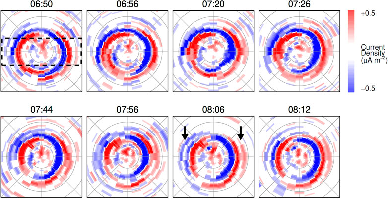
FIGURE 1. A series of eight northern hemisphere polar plots from Sangha et al. (2020), showing the development of AMPERE field-aligned current densities during a FAC bifurcation event, from 06:50 to 08:12 UT on 2 June 2011. The color scale shows upward (red) and downward (blue) FACs, saturating at ±0.5 μA m⁻². The gray concentric rings show the colatitude in steps of 10°, up to 35°. 12 MLT (local noon) is located at the top of the plots, with 06 MLT (dawn) on the right. The dashed box indicates the axis of interest - the dawn-dusk axis. The locations of interest are indicated with the black arrows in the 08:06 UT panel, where there are R2Bs present in both the dawn and dusk regions. The first panel shows the standard R1/R2 pattern, which evolves and by 07:44 UT the polar cap is seen to have contracted, with R2Bs clearly evident ∼25° to 30° (Sangha et al., 2020).

In this paper, we describe further analyses of the occurrence of R2Bs. In Section 2 we describe the instrumentation that has been used for these studies. We then include a more in-depth study of the seasonal variations of the R2Bs in Section 3, as well as the UT dependence that we have discovered in Section 4. We currently do not know the reason for this dependence. However, we mention some possible causes of this distribution in Section 5. We conclude in Section 6.

2 Instrumentation

The work that we present in this paper uses data from AMPERE, collected from the Iridium satellite constellation. Iridium consists of 66 satellites in six polar orbital planes circling the Earth at low altitudes of 780 km. The satellites cross both the North and South polar regions, allowing for the FAC density to be determined for both the northern and southern auroral regions, with a cadence of a few minutes (Anderson et al., 2000, Anderson et al., 2002). The FACs are inferred from measurements of magnetic field perturbations via engineering magnetometers on-board the satellites. These data are used to constrain a spherical harmonic fit, from which the FAC density can be computed (Anderson et al., 2000; Waters et al., 2001; Green et al., 2006; Coxon et al., 2014a, Coxon et al., 2014b, Coxon et al., 2018).

3 Seasonal and Interhemispheric Variability

Sangha et al. (2020) discussed the dawn-dusk and interhemispheric variabilities between the occurrences of the R2Bs. An initial analysis of the seasonal occurrence distribution was also discussed.

Following on from this initial study in Sangha et al. (2020), we now present the results of our complete seasonal analysis. To conduct this study, we identified the number of occurrences of R2Bs throughout 2010 to 2016 during the different seasons. This was done by using data from the months of June and July (northern hemisphere summer solstice), March and September (equinoxes), and December and January (southern hemisphere summer solstice). The R2B occurrences were identified by plotting keograms (time-latitude plots) of the AMPERE data (shown here in Figure 2 and in Figure 5 of Sangha et al. (2020)), and analyzing the plots by eye. The requirements for R2B identification were that the R2 FACs needed to diverge by at least 5° away from the original R2 current, extending above 20° colatitude at dusk and below −20° colatitude at dawn. The R2B had to persist for at least 30 min, and be seen in at least two adjacent MLT sectors.

FIGURE 2

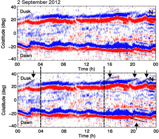
FIGURE 2. An example of an AMPERE FAC keogram used to identify R2Bs. The data were taken from 2 September 2012, in particular the dawn-dusk axis. Upward FACs are shown in red and downward FACs in blue, in the same scale as Figure 1. Both plots are showing the same data, with the second showing the annotated version allowing for the R2Bs to be clearly identified. The arrows indicate the dawn and dusk R2B occurrences at 20 UT and 02, 16, 20, and 22 UT, respectively. The dotted lines follow the evolution of the events throughout the day. The time between the dashed lines (04 and 15 UT) shows the period with no R2B activity occurring.

Figure 2 shows an example of the AMPERE keograms created for the identification of the R2Bs. This example shows FAC data from 2 September 2012, where a small number of R2B events occurred, as well as a period of no R2B activity. These data were taken from the dawn-dusk axis. The direction of the currents are shown in the range of red to blue, where red identifies the upward FACs and blue identifies the downward FACs in the same scale as Figure 1. The top and bottom panels are showing the same keogram, the second of which has been annotated to denote the key features. The arrows indicate the locations of the bifurcations at 02, 16, 20 and 22 UT in the dusk sector, and 20 UT in the dawn sector. The development of the R2B occurrences are shown with the dotted lines within the features. The period between 04 and 15 UT (within the dashed lines) shows no bifurcation activity occurring. The R2Bs can be seen as the R2 current extending to lower latitudes away from the R1/R2 boundary. During the period of no bifurcations, the R2 current remains continuous and alongside the R1 current.

In total, 275 R2B events were observed during June and July, 243 events during March and September, and 216 events during December and January. In each case, we noted if an event was observed simultaneously in both hemispheres, or just in one hemisphere. The proportion of events observed in each hemisphere is summarized in Table 1.

TABLE 1

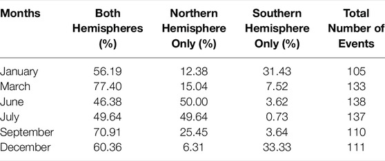
TABLE 1. Table showing the ratio of occurrences of R2Bs in the months of January, December (southern summer solstice), March, September (equinox), and June, July (northern summer solstice).

From the table, we can deduce that on average ∼50% of events are seen in both hemispheres conjugately (this percentage is higher during the months of equinox). Of the events that only appear in one hemisphere, for both the northern and southern summer months, the events favor the summer hemisphere. Specifically, during June/July, ∼50% of R2Bs identified were seen only in the summer hemisphere, with ∼2% of events being seen in the winter hemisphere alone. During December/January, these numbers change to ∼32% of R2B occurrences being seen only in the summer hemisphere, and ∼9% in the winter hemisphere. This suggests that the ionospheric conductance, which is primarily produced by solar illumination, plays a significant role in modulating the occurrence of R2Bs in each hemisphere.

For the equinox months, March and September, we would expect to see events appearing more often than not in both hemispheres simultaneously. This is due to the fact that this time of year is when the ionospheric conductance is most equal between the two hemispheres. This is indeed the case, with ∼75% being seen conjugately. However, those single-hemisphere events seem to have a preference for the northern hemisphere. ∼20% of R2Bs seen in one hemisphere were seen in the northern hemisphere, and ∼6% were identified in the southern hemisphere alone. This is more evident in the autumn equinox than the spring equinox. The autumn equinox saw ∼7% fewer events seen conjugately, and ∼10% more events identified solely in the northern hemisphere. These results suggest that ionospheric conductance plays a predominant role in controlling the occurrence of R2Bs, but that the R2Bs also show a preference for occurring in the northern hemisphere. This is discussed further in Section 5.

4 Bifurcation UT Dependence

In this section, we investigate the UT occurrence of R2Bs for both the northern and southern hemispheres. 24 hour-long bins were used to created this distribution. We used data from 2011 to 2014 for the same seasonal months (Jan/Mar/Jun/Jul/Sep/Dec). In this time period, there were 601 days where AMPERE data were available for both the northern and southern hemispheres, from which the keograms were created and analyzed. If an R2B signature was identified, it was included in this distribution by adding it to the UT bin in which the signature was present. If the same event spanned over multiple hours of UT, the event was incorporated into each UT where the signature was present. For example, if an event was identified at 06 UT, and persisted until 09 UT, then that event would be included in the 06, 07, and 08 UT bins for this distribution. The distributions are shown in Figure 3. The top plot shows the distribution for the R2B events observed in the North, and the bottom plot shows the same for the South. The dawn R2B events are shown in red, and the dusk R2Bs are shown in blue.

FIGURE 3

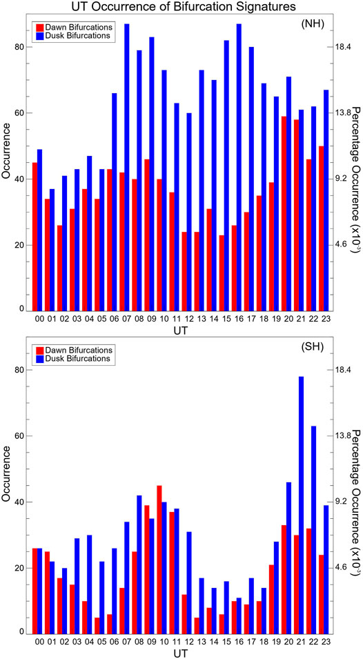
FIGURE 3. Universal time (UT) occurrence distribution of the bifurcation signatures from 2011 to 2014, in (top) the northern hemisphere and (bottom) the southern hemisphere. The right-hand axis shows the percentage occurrence of the R2Bs. In both plots, the red shows the dawn bifurcations and the blue shows the dusk bifurcations.

What is immediately clear when looking at the plots, is that the R2B occurrence rate is not uniformly distributed. The distributions in both hemispheres show two peaks in occurrences at both the dawn and dusk. This could indicate the superposition of two effects–one from the northern hemisphere and one from the southern hemisphere, which are being added together. This would suggest that the R2Bs may then be impacted by conditions in both the northern and southern ionospheres.

The UT distributions were further sub-divided by season; the northern seasonal distributions are shown in Figure 4. The top panel shows the distribution for the R2B events from northern hemisphere winter (December and January), the middle panel shows the R2B events for the northern equinox (March and September), and the last panel shows the R2B events for the northern summer (June and July). In all panels, the red shows the dawnside R2Bs, and the blue shows the duskside R2Bs. By looking at these histograms, we were able to identify the peaks within each of the distributions.

FIGURE 4

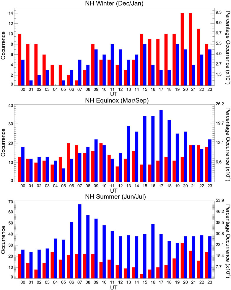
FIGURE 4. The UT occurrence distribution of R2Bs from 2011 to 2014, for the northern hemisphere split by season: (top) northern winter (December/January) (middle) northern equinox (March/September), and (bottom) northern summer (June/July). The right-hand axis shows the percentage occurrence. Red showing dawn and blue showing dusk R2Bs.

Looking at the overall distribution for the northern hemisphere (top plot from Figure 3), we can see the location of the distinct peaks in the distributions. The two peaks in the dawn R2Bs are roughly: 07 UT and 21 UT, with two peaks for the dusk R2Bs being roughly: 07 UT and 16 UT. Looking to the seasons now in Figure 4, one thing to note is the difference in the number of events. The peak number of events in the northern hemisphere winter distribution is 14, whereas in the equinoxes it is 37, and in the summer this peak reaches 67. This further confirms that the FACs favor the summer hemisphere.

As can be seen from Figure 4, almost all of the plots also have the appearance of two peaks in the R2B distributions, with little overlap. Northern hemisphere winter is the only one without a double peaked distribution. It has a single peak in the dawn R2Bs at ∼20 UT, and a clear minima at 04 UT in the dusk R2Bs followed by several peaks of nearly equal magnitude between 09 and 23 UT. However, the distributions for northern hemisphere equinox and summer do present two peaks. For equinox, the dawn peaks are: ∼10 UT and ∼22 UT, and the dusk peaks are: 09 UT and 17 UT. For northern hemisphere summer, the dawn peaks are: ∼08 UT and ∼19 UT, and the dusk peaks are: ∼07 UT and ∼16 UT.

By directly comparing the peaks in the seasonal plots to the total distribution for the northern hemisphere, we can see that they coincide. That is, for the peak in the dawn R2B occurrences from northern hemisphere winter at 20 UT, there is a clear peak in the overall distribution of dawnside events. For the peak in the equinoxes duskside occurrences at 17 UT, there is a peak in the overall distribution of the duskside events at 17 UT also.

We now consider the southern hemisphere distributions. These are shown in Figure 5, in the same layout as Figure 4. We have the southern hemisphere winter at the top, equinox in the middle, and southern hemisphere summer in the bottom panel. The red shows dawnside occurrences, and blue shows duskside occurrences.

FIGURE 5

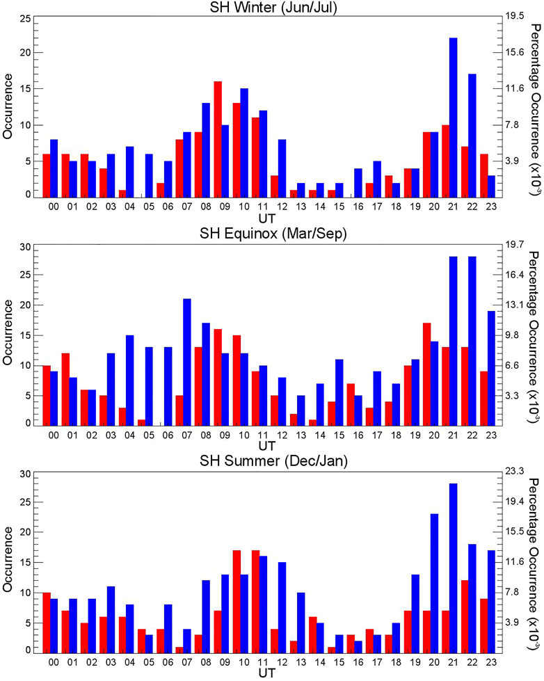
FIGURE 5. The UT occurrence distribution of R2Bs from 2011 to 2014, for the southern hemisphere split by season: (top) southern winter (June/July) (middle) southern equinox (March/September), and (bottom) southern summer (December/January). The right-hand axis shows the percentage occurrence. Red showing dawn and blue showing dusk R2Bs.

The total distribution (bottom panel in Figure 3) shows a clearer double peak than for the northern hemisphere. There are clear dawnside peaks at: 10 UT and 20 UT, and clear duskside peaks at: 08 UT and 21 UT. Initial analysis of the seasonal plots shows a smaller change between the number of peak R2B occurrences between the seasons. Figure 5 shows that southern hemisphere winter has a peak of 22 events, equinox has a peak of 28, and southern hemisphere summer has a peak of 28.

The southern hemisphere UT distributions are more consistent between seasons than in the northern hemisphere. For southern hemisphere winter, the dawnside peaks are: 09 UT and 21 UT, with the duskside peaks being located at: 10 UT and 21 UT. The equinox sees dawnside peaks at: 09 UT and 20 UT, and duskside peaks of: 07 UT and 21 UT. Finally, for southern hemisphere summer, we have dawn peaks at: 10 UT and 22 UT, and duskside peaks at: 11 UT and 21 UT.

These distributions suggest that the occurrence of R2Bs is modulated by hemisphere, season, and UT. It also appears as though both the northern and southern hemispheres contribute to this modulation. One possible explanation is the conductance of the ionospheres, as discussed in the next section.

5 Discussion

In this paper, we have presented the seasonal dependence and UT occurrence of Region 2 Field-Aligned Current Bifurcations (R2Bs). The occurrence of R2Bs maximizes at dawn and dusk, though with a preference for dusk events. R2Bs are observed most frequently in the summer hemisphere suggesting that ionospheric conductance plays a role in modulating the occurrence. Furthermore, the occurrence in UT tends to be double-peaked in both northern and southern hemispheres, possibly with a lower probability of observation when the conductance is a maximum in either hemisphere.

In approximately 50% of occurrences, R2Bs were observed simultaneously in both hemispheres. In the remainder of cases, the events favored the summer hemisphere suggesting that ionospheric conductance, which increases with greater solar illumination, is a significant influencer of R2Bs in each hemisphere.

Furthermore, during the equinoctial months (when the ionospheric conductance is thought to be most similar between the two hemispheres) we would expect the R2Bs to mostly appear in both hemispheres, which is true for ∼74% of the events. We expect the other occurrences to be split relatively evenly between the hemispheres, which is not the case. In fact, of the events seen in a single hemisphere, there were ∼8–22% more seen in the northern hemisphere compared to the southern hemisphere for equinox. This is consistent with the results of Coxon et al. (2016), Laundal et al. (2017), Workayehu et al. (2019) and others, who showed that on average the FACs are stronger in the northern hemisphere than the southern hemisphere. As mentioned in Section 3, the single-hemisphere detected R2Bs show a larger North-South asymmetry in the autumn equinox over the spring equinox. ∼10% more events were shown to have a preference for the northern hemisphere during the autumn equinox over the spring equinox. Work by Workayehu et al. (2020) showed the interhemispheric differences of the FACs varies with season. During local winter and autumn the asymmetry is larger than during local summer and spring, which could be the same effect we are seeing in the occurrences of the R2Bs. During the majority of the time in the southern summer months (December/January), the R2Bs are seen in both hemispheres simultaneously. For the single hemisphere observations, they are more often seen in the southern (summer) hemisphere. However, the difference between occurrences in the northern hemisphere versus the southern hemisphere is smaller for the southern summer than for the northern summer. This suggests that the FAC imbalance between the northern and southern hemisphere is also impacting the occurrence of R2B events.

The UT distributions in the two hemispheres showed two distinct peaks. This could suggest that there are preferred longitudes for the occurrence of R2Bs. However, as the peaks occur at about the same UTs for both dawn and dusk R2Bs, this seems unlikely. Rather, we suggest that the location of the solar terminator is a possible controlling factor, because it will affect dawn and dusk similarly through its influence on ionospheric conductance (i.e., height-integrated conductivity). These double-peaked distributions also suggest that the occurrence of R2Bs is modulated by season and by UT, and that both the northern and southern hemispheres contribute to this modulation. In what follows, we discuss the impact of conductivity on the occurrence of R2Bs, along with other factors which may contribute to a UT dependence, including dayside reconnection geometries and neutral winds.

We start by discussing ionospheric conductance. Enhanced ionospheric conductivity, which is associated with solar illumination, leads to larger FACs (Ohtani et al., 2005). As solar illumination (and ionospheric conductance) is greatest in the summer months, we would expect the R2Bs to be more visible in these months; this is indeed the case. As the Earth rotates, the geomagnetic pole moves towards and away from the Sun, shifting the polar regions towards the sunlight-produced ionospheric conductance. This conductance may be expected to have an influence on R2Bs. The magnetic pole faces towards the Sun at ∼17 UT for the northern hemisphere and 05 UT for the southern hemisphere (Coxon et al., 2016). This means that when the pole is facing the Sun, there is increased solar illumination for that time compared to the rest of the day. This increases the ionospheric conductance in that hemisphere, i.e., in the North the conductance will be a maximum at 17 UT, and in the South it will be maximum at 05 UT. We might, therefore, expect to see a single peak in the northern hemisphere and southern hemisphere at 17 and 05 UT, respectively. However, the peaks that our distributions are showing are: northern hemisphere dawn–07 UT and 21 UT, northern hemisphere dusk–07 UT and 16 UT, southern hemisphere dawn–10 UT and 20 UT, southern hemisphere dusk–08 UT and 21 UT. As there are two peaks seen, it suggests that the conductance in each hemisphere has an influence on the visibility of the R2Bs in both hemispheres. The peaks seen here are slightly offset from the times of the poles pointing towards the Sun suggesting there are other impacting factors involved, some of which are discussed further below.

The predominant focus of this analysis was in reference to the location of the peaks. However, the location of the troughs can be identified as being roughly at 05 and 17 UT, which is clearer to see in the distribution for the southern hemisphere. These are the times corresponding to the southern and northern hemisphere magnetic dipoles pointing toward the Sun, respectively (Coxon et al., 2016). As discussed in Section 1, we believe that R2Bs are connected to SAPS flows. This is because the DMSP SSUSI imager showed the R2Bs occurring in the sub-auroral ionosphere, predominantly in the dusk region, and SuperDARN indicated an association with fast ionospheric flows (Sangha et al., 2020). SAPS are associated with periods of low auroral conductance. During these times of low conductance, the ionospheric polarization electric fields can increase, which leads to SAPS flows forming. However, during the times specified, the conductance increases due to solar illumination, which can suppress this process and reduce the number of SAPS flows.

One reason as to why the conductance in one hemisphere could have an influence on the visibility of R2Bs in the other, is if the R2Bs were forming on closed field lines, impacting both hemispheres simultaneously. Another reason could be that high conductance in one hemisphere may also suppress the R2Bs in both hemispheres. The rise in overall conductance would lead to a smaller region of low conductance (where the R2Bs form). This would explain the small peaks seen midway between 05 and 17 UT, when the conductance is not a maximum in the either hemisphere. However, it is not clear as to why this mechanism would impact the dawn and dusk R2Bs differently. Another possible reason for the difference in behavior between the hemispheres, is that the magnetic pole is displaced further from the rotation pole in the South than in the North, so the UT variation in conductance will be larger (but not by a huge amount) (Bruinsma et al., 2006; Cnossen and Richmond 2012). An increase in conductance during certain hours of UT could cause a decrease in the number of R2B events occurring, as seen in our distributions.

We now discuss dayside reconnection geometries. Increased dayside reconnection ultimately leads to the occurrence of substorms, of which R2Bs seem to be a new facet. Variations in IMF geometry, as it approaches the magnetosphere, can have an impact on reconnection rates. For example, when IMF B_Z is negative, that is the IMF is directed southward, then dayside reconnection increases. Alternatively, changes in the orientation of IMF B_Y can also impact the resulting ionospheric flows and cusp regions (Holzworth and Meng 1984; Erlandson et al., 1988; Candidi et al., 1989; Newell et al., 1989; Cowley et al., 1991). Although we have not currently checked the B_Y dependence of dawn/dusk R2Bs, this would certainly be an interesting avenue for future research. Additionally, the speed of the solar wind has also been seen to impact the rate of dayside reconnection (Milan et al., 2012). Periods of higher dayside reconnection could lead to an increase in R2B events developing. This may be having an impact on the results presented in this paper.

There are seasonal variations that also effect the dayside reconnection rates. Geomagnetic activity peaks are seen roughly at the equinoctial months. The Russell-McPherron effect states that the more southward the IMF, the more magnetic activity occurs. At the equinoxes, geomagnetic activity is increased due to the dipole tilt being the largest (enabling the angle between the IMF and the dipole to be the largest). When the southward component of the IMF is most negative, it can couple more efficiently with the terrestrial magnetic field. This would increase the rate of reconnection, and hence geomagnetic activity. The time of day in which the effective average southward component of the IMF is most negative changes based on what month of the year we are currently in (see Figure 5 in Russell and McPherron (1973)) (Russell and McPherron 1973; Zhao and Zong 2012; Lockwood et al., 2020b). These seasonal variations may be effecting the occurrence of R2Bs.

There are also longitudinal variations in space weather that change as the Earth travels around the Sun. The Earth’s magnetic poles oscillate during the day, moving to point toward and away from the Sun (as already discussed) (Coxon et al., 2016). There are also offsets of the rotational and magnetic poles, which are different in the two hemispheres. These can cause longitudinal variations in space weather (Cnossen and Richmond 2012; Lockwood et al., 2020b,a,c, 2021). Although longitudinal variations may play some role in creating this UT distribution, it is unlikely to cause changes between the longitudes that is drastic enough to account for the UT distribution found.

Finally, we mention neutral winds. Electric fields, and hence ionospheric currents, depend on the relative motion of the ionosphere and neutral background. Neutral winds will influence this relative motion, so can increase or decrease the horizontal currents, in turn affecting the FACs (Lu et al., 1995). Seasonal variations in prevalent neutral winds could hence influence the occurrence of R2Bs. The authors do not currently have an in-depth understanding of these prevalent winds, so will be leaving these for a future study.

Further study is required to understand these UT and seasonal variations of the R2B occurrences.

6 Conclusion

We have confirmed the dawn-dusk and the interhemispheric asymmetry in the occurrence of R2Bs, the proposed FAC signature of SAPS reported in Sangha et al. (2020). The R2Bs favor the dusk region and the summer hemisphere. The occurrence of R2Bs shows an interhemispheric asymmetry: 50% of R2Bs occur simultaneously in both hemispheres, but in other cases they favor the summer hemisphere. There is also a preponderance of R2Bs occurring in the northern hemisphere, reflecting the stronger average FACs observed in the North (Coxon et al., 2016). Similar double-peaked UT occurrence distributions are seen in both hemispheres, with peaks near 09 and 21 UT for both dawn and dusk R2Bs. These suggest that the occurrence of R2Bs in one hemisphere is also influenced by conditions in the conjugate hemisphere. As these R2Bs may be related to the SAPS phenomena, these results may also show a potential relationship between SAPS and seasonal/UT variations. We suggest that ionospheric conductance, controlled by seasonal and UT changes in solar illumination, plays a role in modulating the occurrence of R2Bs. However, the relationship is not a simple one and further work must be done to understand it.

Data Availability Statement

Publicly available datasets were analyzed in this study. This data can be found here: http://ampere.jhuapl.edu.

Author Contributions

HKS identified the Region 2 Bifurcation occurrences, and created the analyses as described in this paper. SEM aided with the methods and analyses of the work, and with editing the paper. BJA and HK provided the data to be analyzed.

Funding

HKS was supported by a studentship from the Science and Technology Facilities Council (STFC), United Kingdom; SEM was supported by STFC grant no. ST/N000749/1.

Conflict of Interest

The authors declare that the research was conducted in the absence of any commercial or financial relationships that could be construed as a potential conflict of interest.

Publisher’s Note

All claims expressed in this article are solely those of the authors and do not necessarily represent those of their affiliated organizations, or those of the publisher, the editors and the reviewers. Any product that may be evaluated in this article, or claim that may be made by its manufacturer, is not guaranteed or endorsed by the publisher.

Acknowledgments

This research used the SPECTRE High Performance Computing Facility at the University of Leicester.

References

Akasofu, S.-I., and Chao, J. K. (1979). Prediction of the Occurrence and Intensity of Magnetospheric Substorms. Geophys. Res. Lett. 6, 897–899. doi:10.1029/GL006i011p00897

CrossRef Full Text | Google Scholar

Anderson, B. J., Takahashi, K., Kamei, T., Waters, C. L., and Toth, B. A. (2002). Birkeland Current System Key Parameters Derived from Iridium Observations: Method and Initial Validation Results. J. Geophys. Res. 107, 1–13. doi:10.1029/2001JA000080

CrossRef Full Text | Google Scholar

Anderson, B. J., Takahashi, K., and Toth, B. A. (2000). Sensing Global Birkeland Currents with Iridium Engineering Magnetometer Data. Geophys. Res. Lett. 27, 4045–4048. doi:10.1029/2000GL000094

CrossRef Full Text | Google Scholar

Bruinsma, S., Forbes, J. M., Nerem, R. S., and Zhang, X. (2006). Thermosphere Density Response to the 20-21 November 2003 Solar and Geomagnetic Storm from CHAMP and GRACE Accelerometer Data. J. Geophys. Res. 111. doi:10.1029/2005JA011284

CrossRef Full Text | Google Scholar

Candidi, M., Mastrantonio, G., Orsini, S., and Meng, C.-I. (1989). Evidence of the Influence of the Interplanetary Magnetic Field Azimuthal Component on Polar Cusp Configuration. J. Geophys. Res. 94, 13585–13591. doi:10.1029/JA094iA10p13585

CrossRef Full Text | Google Scholar

Clausen, L. B. N., Baker, J. B. H., Ruohoniemi, J. M., Greenwald, R. A., Thomas, E. G., Shepherd, S. G., et al. (2012). Large-scale Observations of a Subauroral Polarization Stream by Midlatitude SuperDARN Radars: Instantaneous Longitudinal Velocity Variations. J. Geophys. Res. 117, a–n. doi:10.1029/2011JA017232

CrossRef Full Text | Google Scholar

Cnossen, I., and Richmond, A. D. (2012). How Changes in the Tilt Angle of the Geomagnetic Dipole Affect the Coupled Magnetosphere-Ionosphere-Thermosphere System. J. Geophys. Res. 117, a–n. doi:10.1029/2012JA018056

CrossRef Full Text | Google Scholar

Cowley, S. W. H., and Lockwood, M. (1992). Excitation and Decay of Solar Wind-Driven Flows in the Magnetosphere-Ionosphere System. Ann. Geophysicae 10, 103–115.

Google Scholar

Cowley, S. W. H., Morelli, J. P., and Lockwood, M. (1991). Dependence of Convective Flows and Particle Precipitation in the High-Latitude Dayside Ionosphere on theXandYcomponents of the Interplanetary Magnetic Field. J. Geophys. Res. 96, 5557–5564. doi:10.1029/90JA02063

CrossRef Full Text | Google Scholar

Coxon, J. C., Milan, S. E., and Anderson, B. J. (2018). A Review of Birkeland Current Research Using AMPERE. American Geophysical Union, 257–278. doi:10.1002/9781119324522.ch16

CrossRef Full Text | Google Scholar

Coxon, J. C., Milan, S. E., Carter, J. A., Clausen, L. B. N., Anderson, B. J., and Korth, H. (2016). Seasonal and Diurnal Variations in AMPERE Observations of the Birkeland Currents Compared to Modeled Results. J. Geophys. Res. Space Phys. 121, 4027–4040. doi:10.1002/2015JA022050

CrossRef Full Text | Google Scholar

Coxon, J. C., Milan, S. E., Clausen, L. B. N., Anderson, B. J., and Korth, H. (2014b). A Superposed Epoch Analysis of the Regions 1 and 2 Birkeland Currents Observed by AMPERE during Substorms. J. Geophys. Res. Space Phys. 119, 9834–9846. doi:10.1002/2014JA020500

CrossRef Full Text | Google Scholar

Coxon, J. C., Milan, S. E., Clausen, L. B. N., Anderson, B. J., and Korth, H. (2014a). The Magnitudes of the Regions 1 and 2 Birkeland Currents Observed by AMPERE and Their Role in Solar Wind‐magnetosphere‐ionosphere Coupling. J. Geophys. Res. Space Phys. 119, 9804–9815. doi:10.1002/2014JA020138

CrossRef Full Text | Google Scholar

Daglis, I. A., Thorne, R. M., Baumjohann, W., and Orsini, S. (1999). The Terrestrial Ring Current: Origin, Formation, and Decay. Rev. Geophys. 37, 407–438. doi:10.1029/1999RG900009

CrossRef Full Text | Google Scholar

Dungey, J. W. (1961). Interplanetary Magnetic Field and the Auroral Zones. Phys. Rev. Lett. 6, 47–48. doi:10.1103/PhysRevLett.6.47

CrossRef Full Text | Google Scholar

Eastman, T. E., Frank, L. A., Peterson, W. K., and Lennartsson, W. (1984). The Plasma Sheet Boundary Layer. J. Geophys. Res. 89, 1553–1572. doi:10.1029/JA089iA03p01553

CrossRef Full Text | Google Scholar

Erlandson, R. E., Zanetti, L. J., Potemra, T. A., Bythrow, P. F., and Lundin, R. (1988). IMFBydependence of Region 1 Birkeland Currents Near Noon. J. Geophys. Res. 93, 9804–9814. doi:10.1029/JA093iA09p09804

CrossRef Full Text | Google Scholar

Foster, J. C., and Burke, W. J. (2002). SAPS: A New Categorization for Sub-auroral Electric fields. Eos Trans. AGU 83, 393–394. doi:10.1029/2002EO000289

CrossRef Full Text | Google Scholar

Green, D. L., Waters, C. L., Anderson, B. J., Korth, H., and Barnes, R. J. (2006). Comparison of Large-Scale Birkeland Currents Determined from Iridium and SuperDARN Data. Ann. Geophys. 24, 941–959. doi:10.5194/angeo-24-941-2006

CrossRef Full Text | Google Scholar

Holzworth, R. H., and Meng, C.-I. (1984). Auroral Boundary Variations and the Interplanetary Magnetic Field. Planet. Space Sci. 32, 25–29. doi:10.1016/0032-0633(84)90038-2

CrossRef Full Text | Google Scholar

Huang, C., Sazykin, I., Spiro, R., Goldstein, J., Crowley, G., and Ruohoniemi, J. M. (2006). Storm-time Penetration Electric fields and Their Effects. Eos Trans. AGU 87, 131. doi:10.1029/2006EO130005

CrossRef Full Text | Google Scholar

Iijima, T., and Potemra, T. A. (1976b). Field-aligned Currents in the Dayside Cusp Observed by Triad. J. Geophys. Res. 81, 5971–5979. doi:10.1029/JA081i034p05971

CrossRef Full Text | Google Scholar

Iijima, T., and Potemra, T. A. (1978). Large-scale Characteristics of Field-Aligned Currents Associated with Substorms. J. Geophys. Res. 83, 599–615. doi:10.1029/JA083iA02p00599

CrossRef Full Text | Google Scholar

Iijima, T., and Potemra, T. A. (1976a). The Amplitude Distribution of Field-Aligned Currents at Northern High Latitudes Observed by Triad. J. Geophys. Res. 81, 2165–2174. doi:10.1029/JA081i013p02165

CrossRef Full Text | Google Scholar

Laundal, K. M., Cnossen, I., Milan, S. E., Haaland, S. E., Coxon, J., Pedatella, N. M., et al. (2017). North-south Asymmetries in Earth's Magnetic Field. Space Sci. Rev. 206, 225–257. doi:10.1007/s11214-016-0273-0

CrossRef Full Text | Google Scholar

Lejosne, S., and Mozer, F. S. (2017). Subauroral Polarization Streams (SAPS) Duration as Determined from Van Allen Probe Successive Electric Drift Measurements. Geophys. Res. Lett. 44, 9134–9141. doi:10.1002/2017GL074985

CrossRef Full Text | Google Scholar

Lockwood, M., Haines, C., Barnard, L. A., Owens, M. J., Scott, C. J., Chambodut, A., et al. (2021). Semi-annual, Annual and Universal Time Variations in the Magnetosphere and in Geomagnetic Activity: 4. Polar Cap Motions and Origins of the Universal Time Effect. J. Space Weather Space Clim. 11, 15. doi:10.1051/swsc/2020077

CrossRef Full Text | Google Scholar

Lockwood, M., McWilliams, K. A., Owens, M. J., Barnard, L. A., Watt, C. E., Scott, C. J., et al. (2020a). Semi-annual, Annual and Universal Time Variations in the Magnetosphere and in Geomagnetic Activity: 2. Response to Solar Wind Power Input and Relationships with Solar Wind Dynamic Pressure and Magnetospheric Flux Transport. J. Space Weather Space Clim. 10, 30. doi:10.1051/swsc/2020033

CrossRef Full Text | Google Scholar

Lockwood, M., Owens, M. J., Barnard, L. A., Haines, C., Scott, C. J., McWilliams, K. A., et al. (2020b). Semi-annual, Annual and Universal Time Variations in the Magnetosphere and in Geomagnetic Activity: 1. Geomagnetic Data. J. Space Weather Space Clim. 10, 23. doi:10.1051/swsc/2020023

CrossRef Full Text | Google Scholar

Lockwood, M., Owens, M. J., Barnard, L. A., Watt, C. E., Scott, C. J., Coxon, J. C., et al. (2020c). Semi-annual, Annual and Universal Time Variations in the Magnetosphere and in Geomagnetic Activity: 3. Modelling. J. Space Weather Space Clim. 10, 61. doi:10.1051/swsc/2020062

CrossRef Full Text | Google Scholar

Lu, G., Richmond, A. D., Emery, B. A., and Roble, R. G. (1995). Magnetosphere-ionosphere-thermosphere Coupling: Effect of Neutral Winds on Energy Transfer and Field-Aligned Current. J. Geophys. Res. 100, 19643–19659. doi:10.1029/95JA00766

CrossRef Full Text | Google Scholar

McPherron, R. L. (1979). Magnetospheric Substorms. Rev. Geophys. 17, 657–681. doi:10.1029/RG017i004p00657

CrossRef Full Text | Google Scholar

McPherron, R. L. (1991). “Physical Processes Producing Magnetospheric Substorms and Magnetic Storms,” in Geomagnetism. Editor J. A. Jacobs (Cambridge, MA: Academic Press), 593–739. doi:10.1016/b978-0-12-378674-6.50013-3

CrossRef Full Text | Google Scholar

Milan, S. E., Clausen, L. B. N., Coxon, J. C., Carter, J. A., Walach, M.-T., Laundal, K., et al. (2017). Overview of Solar Wind-Magnetosphere-Ionosphere-Atmosphere Coupling and the Generation of Magnetospheric Currents. Space Sci. Rev. 206, 547–573. doi:10.1007/s11214-017-0333-0

CrossRef Full Text | Google Scholar

Milan, S. E., Gosling, J. S., and Hubert, B. (2012). Relationship between Interplanetary Parameters and the Magnetopause Reconnection Rate Quantified from Observations of the Expanding Polar Cap. J. Geophys. Res. 117, a–n. doi:10.1029/2011JA017082

CrossRef Full Text | Google Scholar

Milan, S. E., Provan, G., and Hubert, B. (2007). Magnetic Flux Transport in the Dungey Cycle: A Survey of Dayside and Nightside Reconnection Rates. J. Geophys. Res. 112, a–n. doi:10.1029/2006JA011642

CrossRef Full Text | Google Scholar

Newell, P. T., Meng, C.-I., Sibeck, D. G., and Lepping, R. (1989). Some Low-Altitude Cusp Dependencies on the Interplanetary Magnetic Field. J. Geophys. Res. 94, 8921–8927. doi:10.1029/JA094iA07p08921

CrossRef Full Text | Google Scholar

Ohtani, S., Ueno, G., and Higuchi, T. (2005). Comparison of Large-Scale Field-Aligned Currents under Sunlit and Dark Ionospheric Conditions. J. Geophys. Res. 110. doi:10.1029/2005JA011057

CrossRef Full Text | Google Scholar

Rostoker, G., Akasofu, S.-I., Foster, J., Greenwald, R. A., Kamide, Y., Kawasaki, K., et al. (1980). Magnetospheric Substorms-Definition and Signatures. J. Geophys. Res. 85, 1663–1668. doi:10.1029/JA085iA04p01663

CrossRef Full Text | Google Scholar

Russell, C. T., and McPherron, R. L. (1973). Semiannual Variation of Geomagnetic Activity. J. Geophys. Res. 78, 92–108. doi:10.1029/JA078i001p00092

CrossRef Full Text | Google Scholar

Sangha, H., Milan, S. E., Carter, J. A., Fogg, A. R., Anderson, B. J., Korth, H., et al. (2020). Bifurcated Region 2 Field-Aligned Currents Associated with Substorms. J. Geophys. Res. Space Phys. 125, e2019JA027041. doi:10.1029/2019JA027041

CrossRef Full Text | Google Scholar

Waters, C. L., Anderson, B. J., and Liou, K. (2001). Estimation of Global Field Aligned Currents Using the Iridium System Magnetometer Data. Geophys. Res. Lett. 28, 2165–2168. doi:10.1029/2000GL012725

CrossRef Full Text | Google Scholar

Workayehu, A. B., Vanhamäki, H., and Aikio, A. T. (2019). Field‐Aligned and Horizontal Currents in the Northern and Southern Hemispheres from the Swarm Satellite. J. Geophys. Res. Space Phys. 124, 7231–7246. doi:10.1029/2019JA026835

CrossRef Full Text | Google Scholar

Workayehu, A. B., Vanhamäki, H., and Aikio, A. T. (2020). Seasonal Effect on Hemispheric Asymmetry in Ionospheric Horizontal and Field-Aligned Currents. J. Geophys. Res. Space Phys. 125, e2020JA028051. doi:10.1029/2020JA028051

CrossRef Full Text | Google Scholar

Zhao, H., and Zong, Q.-G. (2012). Seasonal and Diurnal Variation of Geomagnetic Activity: Russell-Mcpherron Effect during Different IMF Polarity And/or Extreme Solar Wind Conditions. J. Geophys. Res. 117, a–n. doi:10.1029/2012JA017845

CrossRef Full Text | Google Scholar