Recent Applications of Bayesian Methods to the Solar Corona

1 Introduction

The aim of this paper is to give a rationale for the use of Bayesian methods in the study of the solar corona and to show recent applications in the area of solar coronal seismology. Coronal seismology aims to infer difficult to measure physical parameters in magnetic and plasma structures, such as coronal loops and prominence plasmas, by a combination of observations of wave activity and theoretical models, usually under the MHD approximation (Uchida, 1970; Roberts et al., 1984). Because of our lack of direct access to the physical systems of interest information is incomplete and uncertain. As a consequence, solar atmospheric seismology deals with inversion problems that are probabilistic in nature and our conclusions can only be probabilities at best. A prototypical example is the determination of the magnetic field strength in coronal loops from the observational measurement of the kink speed of transverse oscillations (Nakariakov and Ofman, 2001). Only after assumptions about the loop plasma density and the density contrast one can derive the magnetic field. Since the values of the density and density contrast have probabilistic distributions, the derived magnetic field has a probabilistic distribution.

Bayesian analysis is increasingly being used in astrophysics. Figure 1 shows the number of Bayesian astrophysics papers as a function of year. The first studies (already 50 years ago) dealt with both technical problems, such as the construction of image restoration algorithms (Richardson, 1972), as well as with procedures for formalising the evaluation of astrophysical hypotheses by comparison between theoretical predictions and observational data (Sturrock, 1973). It took two more decades for the Bayesian approach to be adopted in solar physics. Initial solar applications were focused on statistical analyses of solar neutrino data (Gates et al., 1995), followed by studies on solar flare prediction (Wheatland, 2004), the analysis of solar global oscillations (Marsh et al., 2008), and the inversion of magnetic and thermodynamic properties of the solar atmosphere from the analysis of spectro-polarimetric data (Asensio Ramos et al., 2007). The first study that made use of Bayesian analysis in coronal seismology was by Arregui and Asensio Ramos (2011), who inferred coronal loop physical parameters from observed periods and damping times of their transverse oscillations. In the last decade, about 25 studies in coronal seismology have made use of Bayesian techniques. They deal with parameter inference, model comparison, and model averaging applications to gain information on the magnetic field and the plasma conditions in structures in the solar corona and in solar prominences. Here, we discuss some recent developments in the area.

FIGURE 1

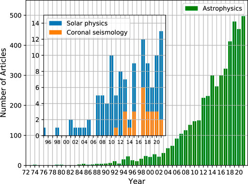
FIGURE 1. Bar plots representing the yearly number of referred articles employing Bayesian analysis techniques in the field of astrophysics, the branch of solar physics, and the research area of coronal seismology. At the time of writing (November 2021), the total number of articles amounts to 4678 in astrophysics, 114 in solar physics, and 25 in coronal seismology. Source: NASA Astrophysics Data System (ADS), digital library operated by the Smithsonian Astrophysical Observatory (SAO).

The layout of the article is the following. Section 2 describes the basic principles and the tools used to perform parameter inference and model comparison in the Bayesian framework. In Section 3, first, results on the inference of physical parameters in coronal loops and prominence plasmas are described. Then, examples are shown on the application of model comparison to the assessment of the damping mechanism(s) of coronal waves. A summary is presented in Section 4.

2 Basic Principles of Bayesian Inference and Model Comparison

Bayesian analysis considers any inversion problem, in terms of probabilistic inference, as the task of estimating the degree of belief on statements about parameter values or model evidence, conditional on observed data. It uses Bayes’ rule (Bayes and Price, 1763),

$p\left(\theta |d,M\right)=\frac{p\left(d|\theta ,M\right)p\left(\theta |M\right)}{\int p\left(d|\theta ,M\right)p\left(\theta |M\right)d\theta },(1)$

which says that our state of knowledge about a set of parameters θ of a given model M, conditional on the observed data d, is a combination of what we know independently of the data, the prior p(θ|M), and the likelihood of obtaining a given data realisation as a function of the parameter vector, the likelihood function p(d|θ, M). Their combination gives the posterior distribution, p(θ|d, M), that encloses all the information about the set of parameters conditional on the observed data and the assumed model. The prior and the likelihood function need to be directly assigned in order to compute the posterior. Bayes’ rule offers a tool to perform rational inference based on the combination of conditional probability distributions. The tool can be applied at three different levels.

In parameter inference the global posterior is computed for the full set of N parameters, θ = {θ₁, …, θ_i, …, θ_N}, and is then marginalised to obtain information about the one of interest. This is achieved by integration of the full posterior with respect to the remaining parameters,

$p\left({\theta }_i|d\right)=\int p\left(\theta |d\right)d{\theta }_1\dots ,d{\theta }_{i-1}d{\theta }_{i+1}\dots ,d{\theta }_N.(2)$

This is the so-called marginal posterior for model parameter θ_i, which contains all the information available in the priors and the data. The uncertainty of the rest of parameters to the one of interest is correctly propagated by this procedure. To summarise the result one can then provide the mean, the mode, the median, etc. It is common to provide the maximum a posteriori estimate of the inferred parameter, ${\theta }_i^{\text{MAP}}$, the value of θ_i that makes the posterior the largest together with credible regions containing a particular fraction of the mass of the distribution. A simple way of computing such credible region is to sort the probability values p(θ_i|d) in descending order. Then, starting with the largest one, add successively smaller values of p(θ_i|d) until the next value would exceed the desired value of e.g., 68%. At each step, one needs to keep track of the corresponding θ_i values. The credible region is then the range in parameter space that includes all the θ_i values corresponding to the p(θ_i|d) values that were added. The boundaries of the credible region give the lower and upper errors. They are the smallest and largest values of θ_i obtained by this procedure. The process of marginalisation can also be applied to the so-called nuisance parameters, those that must be incorporated in the modelling but are not of immediate interest.

The denominator in Eq. 1 is the so-called marginal likelihood or evidence,

$p\left(d|M\right)={\int }_{\theta }p\left(\theta ,d|M\right)d\theta ={\int }_{\theta }p\left(d|\theta ,M\right)p\left(\theta |M\right)d\theta ,(3)$

an integral of the joint distribution of parameters and data over the full parameter space that normalises the likelihood function to turn the result into a probability. It plays a crucial role in model comparison because it is a measure of relational evidence. The measure of evidence is relational because it examines a relation between the predictions by model M and the observed data d. The marginal likelihood quantifies the evidence for a model in relation to the data that it predicts. The general aim of model comparison is to assess the relative evidence between alternative models in explaining the same data. Given two models, M₁ and M₂, this is achieved with the calculation of the posterior ratio p(M₁|d)/p(M₂|d). If the two models are equally probable a priori, p(M₁) = p(M₂), and the posterior ratio is equal to the ratio of marginal likelihoods of the two models

$B_{12}=2\log \frac{p\left(M_1|d\right)}{p\left(M_2|d\right)}=2\log \frac{p\left(d|M_1\right)}{p\left(d|M_2\right)}=-B_{21},(4)$

where the logarithmic scale is used to translate Bayes factors into levels of evidence. The Bayes factors B₁₂ and B₂₁ defined in Eq. 4 measure relative evidence. They quantify the relative plausibility of each of the two models to explain the same data. To evaluate the levels of evidence an empirical table, such as the one by Kass and Raftery (1995), is employed. For values of B₁₂ from 0 to 2, the evidence in favour of model M₁ in front of model M₂ is inconclusive; for values from 2 to 6, positive; for values from 6 to 10, strong; and for values above 10, very strong. A similar tabulation applies to B₂₁.

After a model comparison procedure has been performed, it may be the case that the evidence in favour of any of the models under consideration is not large enough to deem positive evidence. A convenient solution is then to consider the third level of Bayesian inference, model averaging. This is a procedure that combines the posteriors inferred with each model to calculate a model-averaged posterior,

$p\left({\theta }_i|d\right)=\sum _{k}p\left({\theta }_i|d,M_k\right)p\left(M_k|d\right),(5)$

weighted with the evidence for each model. In this manner, parameter constraints that account for the uncertainty about the models are obtained. Such a calculation makes use of all the available information in the data and models in a fully consistent manner. The resulting marginal posteriors are the best inference one can obtain with the available information.

3 Recent Applications to the Solar Corona

After the first application of Bayesian methods to coronal seismology by Arregui and Asensio Ramos (2011), most of the initial studies made use of simple forward models for the prediction of oscillation properties of magnetic structures, such as periods and damping times, and integration over a grid of points in low-dimensional parameter and data spaces (see e.g., Arregui et al., 2013a,b; Asensio Ramos and Arregui, 2013; Arregui and Asensio Ramos, 2014; Arregui and Soler, 2015; Arregui et al., 2015; Arregui and Goossens, 2019). Other studies considered the analysis of the time series of displacement amplitude of oscillations to infer equilibrium properties of coronal loops (see e.g., Pascoe et al., 2017a,b; Pascoe et al., 2018; Goddard et al., 2018). A review summarising those initial applications can be found in Arregui (2018). Additional developments were possible by the creation and application of data analysis tools based on Markov Chain Monte Carlo sampling of posterior distributions (see e.g., Goddard et al., 2017; Pascoe et al., 2017c, 2019; Duckenfield et al., 2019; Pascoe et al., 2020b,a). Details about these methods and their use as diagnostic tools for coronal seismology can be found in Anfinogentov et al. (2021b,a). In the following, we discuss some recent results, focusing on the inference of physical parameters in coronal loops and prominence plasmas and on the damping of transverse oscillations in coronal loops and extended regions of the solar corona.

3.1 Inferring the Magnetic Field Strength and Plasma Density in Coronal Loops

The first modern application of coronal seismology was presented by Nakariakov and Ofman (2001). By interpreting the transverse coronal loop oscillations observed with the Transition Region and Coronal Explorer (TRACE) as the fundamental kink mode of a magnetic flux tube in the long wavelength limit, they showed how the combination of observed period (P) and loop length (L) can enable to constrain the magnetic field strength. The procedure starts with the assumption of a simple expression, model M₁, for the phase speed of the kink mode as a function of the Alfvén speed in the interior of the loop, $v_{\text{Ai}}=B_0/\sqrt{{\mu }_0{\rho }_{\text{i}}}$, and the density contrast, ζ = ρ_i/ρ_e,

$v_{\text{ph}}=v_{\text{Ai}}{\left(\frac{2\zeta }{1+\zeta }\right)}^{1/2},(6)$

with μ₀ the magnetic permeability and ρ_{i, e} the internal and external densities. This expression is valid assuming coronal loops can be modelled as one-dimensional density enhancements in cylindrical coordinates with the magnetic field pointing along the axis of the tube and under the long wavelength approximation. Adopting a given value for the density contrast, ζ, the observationally estimated phase speed (v_ph ∼ 2L/P) enables to obtain the Alfvén speed v_Ai. By further assuming values of loop density on a given range, a range of magnetic field strength values is obtained.

In their Bayesian analysis, Arregui et al. (2019) showed that the problem can be formulated in terms of the inference of a three-dimensional posterior from one observable with the use of Bayes’ rule as the product of likelihood and prior,

$p\left(\left\{{\rho }_{\text{i}},\zeta ,B_0\right\}|v_{\text{ph}},M_1\right\}\sim p\left(v_{\text{ph}}|\left\{{\rho }_{\text{i}},\zeta ,B_0\right\},M_1\right)p\left(\left\{{\rho }_{\text{i}},\zeta ,B_0\right\}|M_1\right).$

Considering a particular observed event, a Gaussian likelihood function and uniform prior distributions for the three unknown parameters, θ = {ρ_i, ζ, B₀}, over plausible ranges leads to the marginal posterior distribution for the magnetic field strength shown in Figure 2A. The result shows that not all values in the range found by Nakariakov and Ofman (2001) are equally probable. A well constrained marginal posterior is obtained which specifies the particular plausibility for each value of the magnetic field strength in the range. From this, estimates with asymmetric error bars can be obtained. Regarding the other two parameters, the density contrast and the loop density, their distribution does not permit to obtain constrained information on their most probable values. The marginal posterior for the magnetic field strength incorporates the uncertainty on these two parameters and can still be properly inferred, even if the values of plasma density inside and outside the coronal loops are highly uncertain.

FIGURE 2

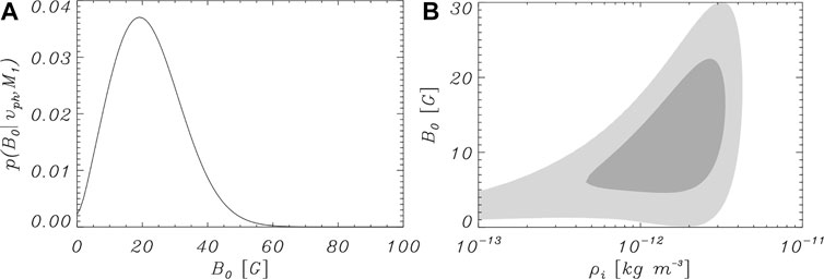
FIGURE 2. (A) Posterior probability distribution for the magnetic field strength for a loop oscillation event with observed phase speed v_ph = 1,030 ± 410 km s⁻¹ under model M₁, given by Eq. 6. The inferred median value for the magnetic field strength is $B_0=21_{-9}^{+12}$ G, with uncertainties given at the 68% credible interval. (B) Joint two-dimensional posterior distribution for the internal density of the waveguide and the magnetic field strength obtained for the inference with a Gaussian prior for the internal density centred at ${\mu }_{{\rho }_{\text{i}}}=1.9\times 10^{-12}$ kg m⁻³ and with ${\sigma }_{{\rho }_{\text{i}}}=0.5{\mu }_{{\rho }_{mathrmi}}$. The inference with the more informative prior on density leads to $B_0=13_{-6}^{+7}$ G and ${\rho }_{\text{i}}=(2.2_{-0.9}^{+0.9})\times 10^{-12}$ kg m⁻³. The outer boundaries of the light grey and dark grey shaded regions indicate the 95% and 68% credible regions, respectively. From Arregui et al. (2019).

One advantage of the Bayesian approach is that it offers a self-consistent way to update the posteriors when additional information is available. Spectroscopic measurements enable us to obtain information about physical properties of the coronal plasma, such as the density. Consider we have some estimate for the density inside the oscillating loop. This additional information can be added to the inference in the form of a Gaussian prior for the density, centred in the measured value. Figure 2B shows the joint posterior for plasma density and magnetic field strength for such an inference, with grey-shaded areas indicating the 68% and 95% credible regions, respectively. This example shows that the inclusion of additional information enables us to better constrain our estimates for the magnetic field strength and plasma density.

Observations show that transverse coronal loop oscillations are quickly damped, with characteristic damping times of a few oscillatory periods. Arregui et al. (2019) evaluated the influence of this observable on the inference of the magnetic field strength. The simplest available and more commonly accepted model is damping by resonant absorption due to the inhomogeneity of the plasma in the cross-field direction (Goossens et al., 2002; Ruderman and Roberts, 2002). Under the thin tube and thin boundary approximations, with a non-uniform layer of width l much shorter than the tube radius R (l ≪ R), the damping time is given by

${\tau }_{\text{d}}\left({\rho }_{\text{i}},\zeta ,B_0,l/R\right)=\frac{2}{\pi }\left(\frac{\zeta +1}{\zeta -1}\right)\left(\frac{1}{l/R}\right)\left(\frac{2L}{v_{\text{ph}}}\right).(7)$

The forward predictions of this new model M₂, given by Eqs 6, 7, are coupled, hence some degree of influence is expected in the inference of the magnetic field, due to the consideration of wave damping. Now the problem can be formulated in terms of the inference of a four-dimensional posterior from three observables with the use of Bayes’ rule as the product of likelihood and prior,

$p\left(\left\{{\rho }_{\text{i}},\zeta ,B_0,l/R\right\}|\left\{v_{\text{ph}},{\tau }_{\text{d}},L\right\},M_2\right)\sim p\left(\left\{v_{\text{ph}},{\tau }_{\text{d}},L\right\}|\left\{{\rho }_{\text{i}},\zeta ,B_0,l/R\right\},M_2\right)p\left(\left\{{\rho }_{\text{i}},\zeta ,B_0,l/R\right\}|M_2\right).$

Considering the same observed event as before, a Gaussian likelihood function and uniform prior distributions for the four unknown parameters, θ = {ρ_i, ζ, B₀.L}, over plausible ranges leads to the results displayed in Figure 3. The resulting marginal posteriors for the magnetic field strength for different damping times show little differences. The advantage of including the damping into the inference is that it enables to infer information on the transverse inhomogeneity length scale of the density at the boundary of the waveguide. This parameter is relevant in the context of wave dissipation processes (Arregui, 2015).

FIGURE 3

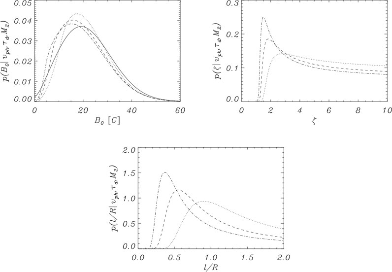
FIGURE 3. Marginal posterior distributions for magnetic field strength, density contrast, and transverse inhomogeneity length scale for the inversion of the problem with forward model given by Eqs 6, 7, a transverse oscillation with v_ph = 1,030 ± 410 km s⁻¹ and different values for the damping time: no damping (solid line), τ_d = 500 s (dotted line), τ_d = 800 s (dashed line), and τ_d = 1,200 s (dash-dotted line) with an associated uncertainty of 50 s in all cases. The inferred medians with errors at the 68% credible interval are $B_0=21_{-9}^{+12}$ G for the undamped case, $B_0=20_{-8}^{+11}$ G for τ_d = 500 s, $B_0=19_{-8}^{+11}$ G for τ_d = 800 s, and $B_0=18_{-9}^{+11}$ G for τ_d = 1,200 s. A fixed value for the loop length L = 1.9 × 10¹⁰ cm was considered in all computations. Adapted from Arregui et al. (2019).

3.2 Inferring the Magnetic Field Strength and Thread Length in Prominences

Bayesian methods are also being applied in prominence seismology. Estimates of periods and phase speeds of propagating waves were obtained by Lin et al. (2009) for a number of threads in a prominence. A fundamental difference in the solution to the inverse problem, in comparison to the case with coronal loops, is that the internal prominence density is two orders of magnitude larger than the external coronal density. This makes the kink speed independent of the density contrast and simplifies Eq. 6 to the approximate expression $v_{\text{ph}}\sim \sqrt{2}{v}_{\text{Ai}}$. By using this fact, Lin et al. (2009) were able to provide estimates for the magnetic field strength in the threads, upon assuming a given value for their plasma density.

Figure 4A gives ranges of variation for the magnetic field strength in 10 selected threads as a function of the prominence density computed by Montes-Solís and Arregui (2019) from data in Table 1 of Lin et al. (2009). From the Bayesian perspective, as in the case of coronal loops, all those values within the obtained ranges are not equally probable. The Bayesian solutions computed by Montes-Solís and Arregui (2019) in the form of marginal posteriors for each of the 10 threads are shown in Figure 4B. For each thread, the magnetic field strength can be properly inferred (see Table 2 in Montes-Solís and Arregui 2019). The distributions spread over a range of values from 1 to 20 G and seem to point to a highly inhomogeneous nature of the studied prominence area. Montes-Solís and Arregui (2019) continue their analysis with the computation of the joint two-dimensional posterior for magnetic field strength and prominence density which, in the case of a Gaussian prior for the density, is well constrained (see Figure 4C).

FIGURE 4

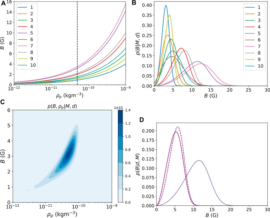
FIGURE 4. (A) Curves obtained for each thread observed by Lin et al. (2009). (B) Posterior distributions of magnetic field strength (B) for each considered thread obtained with Bayesian methods. (C) Global posterior computed for the fifth thread, considering a Gaussian prior of the internal density (ρ_i) centred in a value equal to ρ_p = 5 × 10⁻¹¹ kg m⁻³ and given an uncertainty of 50%. (D) Comparison of posterior distributions of the magnetic field strength in a totally filled tube (purple line), partially filled tube (magenta line), and partially filled tube considering a Gaussian prior for the proportion of thread length centred in L_p/L = 0.5 with 50% of uncertainty (dashed magenta line). From Montes-Solís and Arregui (2019).

In contrast to the case of coronal loops, prominence threads do not occupy the entire length of the magnetic flux tube. We only observe the cold and dense plasma occupying a fraction of a longer but unobservable structure. Soler et al. (2010) constructed a model that provides us with an approximate analytical expression for the phase speed of kink modes in partially filled tubes

$v_{\text{ph}}^{\text{par}}=\frac{2}{\pi \sqrt{\frac{L_{\text{p}}}{L}\left(1-\frac{L_{\text{p}}}{L}\right)}}{v}_{\text{ph}}^{\text{tot}}(8)$

in terms of the phase speed in a totally filled tube, $v_{\text{ph}}^{\text{tot}}=\sqrt{2}{v}_{\text{Ai}}$, with L_p the length of the thread and L the length of the flux tube. Figure 4D shows results for the inference of the magnetic field strength performed for different models for the density along the thread considering: a fully filled tube, a partially filled tube with a uniform prior distribution for L_p/L, and a partially filled tube with a Gaussian prior distribution for L_p/L. The results indicate the importance of having an approximate idea about the ratio L_p/L in order to obtain an accurate inference.

Even in the case of a fully filled tube, L_p = L, as in the case with coronal loops, the inferred posterior for the magnetic field strength is dependent on the amount of information we have on the value of plasma density. Figure 5 shows marginal posteriors for the magnetic field strength corresponding to thread # 5 in Table 2 of Montes-Solís and Arregui (2019). They were calculated with three different priors for the density. One considers a uniform prior. The other two Gaussian distributions centred at two different density values. The results indicate that the obtained posteriors clearly differ.

FIGURE 5

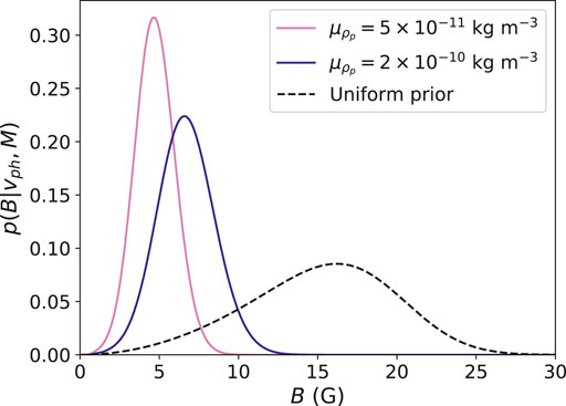
FIGURE 5. Posterior distributions of the magnetic field strength (B) in a fully filled magnetic thread considering a Gaussian prior for the internal density (ρ_i) with mean ${\mu }_{{\rho }_{\text{p}}}=5\times 10^{-11}$ kg m⁻³ (pink), a Gaussian prior with mean ${\mu }_{{\rho }_{\text{p}}}=2\times 10^{-10}$ kg m⁻³ (blue), and a uniform prior (black dashed line). Uncertainties in Gaussian priors are considered to be of 50%. From Montes-Solís and Arregui (2019).

One of the reasons why prominence seismology is in a less developed stage than coronal loop seismology is because there are fewer observations of transverse oscillations in these structures, but also because of the complexity in their modelling. As in prominence threads we only observe the cold and dense part of a longer but unobservable structure, the length of the flux tube cannot be directly estimated. However, using seismology diagnostics with multiple periods one can obtain posterior probability distributions for the ratio of the length of the thread to the length of the flux tube, L_p/L. Also, a number of observations show that threads oscillate and flow simultaneously. This affects the oscillation period which changes in time. By measuring the period at two different moments and using theoretical developments by Soler and Goossens (2011) a number of parameters, such as the flow speed, the length of the thread and the length of the flux tube can be inferred. Applications of these principles can be found in the study by Montes-Solís and Arregui (2019).

3.3 Assessing Damping Mechanisms for Coronal Loop Oscillations

The damping of magnetohydrodynamic waves has been a matter of interest since the first imaging observations of transverse coronal loop oscillations (Aschwanden et al., 1999; Nakariakov et al., 1999). Of particular interest in explaining the observations are the mechanisms based on the cross-field inhomogeneity of the waveguides, such as phase mixing and resonant absorption (Heyvaerts and Priest, 1983; Goossens et al., 2002; Ruderman and Roberts, 2002; Goossens et al., 2006), or those involving lateral or foot-point leakage of wave energy (Spruit, 1982; Roberts, 2000; De Pontieu et al., 2001; Cally, 2003).

Attempts to discriminate between alternative mechanisms were initially focused on the computation of the damping time scales predicted by each mechanism for plausible values of the unknown relevant physical parameters. This approach enables for instance to discard viscous or resistive processes because of the too long timescales they predict. Ofman and Aschwanden (2002) proposed a method based on the comparison between theoretically predicted and fitted power-law indexes between periods and damping times to assess the plausibility of alternative damping mechanisms. This suggestion is based on the assumption that each mechanism is characterised by a particular power-law index, a premise that was shown to be questionable by Arregui et al. (2008). For instance, resonant absorption is able to generate data realisations leading to different scaling laws with different power-law indexes.

A Bayesian approach to comparing the relative plausibility among several proposed damping mechanisms for coronal loop oscillations was followed by Montes-Solís and Arregui (2017). They considered the mechanisms of resonant absorption in the Alfvén continuum (Goossens et al., 2002), phase mixing of Alfvén waves (Heyvaerts and Priest, 1983), and wave leakage of the principal leaky mode (Cally, 2003).

For resonant damping, the theoretically predicted damping time τ_d over the period P, under the thin tube and thin boundary approximations, reads (Goossens et al., 2002; Ruderman and Roberts, 2002)

$\frac{{\tau }_{\text{d}}}{P}=\frac{2}{\pi }\frac{R}{l}\frac{\zeta +1}{\zeta -1},(9)$

with l the thickness of the non-uniform layer at the boundary of the loop and ζ = ρ_i/ρ_e the density contrast between the internal and external densities. Plausible ranges of variation for the unknown parameters are ζ ∈ (1, 10] and l/R ∈ (0, 2]. They are capable of producing the observed fast damping.

For phase mixing, an analytical expression for the damping ratio was derived by Roberts (2000).

$\frac{{\tau }_{\text{d}}}{P}={\left(\frac{3}{{\pi }^2\nu }\right)}^{1/3}{w}^{2/3}{P}^{-1/3}.(10)$

Here ν = 4 × 10³ km² s⁻¹ is the coronal kinematic shear viscosity coefficient and w the transverse inhomogeneity length scale. Considering values of the unknown parameter in the range w ∈ [0.5, 6], the required observed damping times scales can be well reproduced.

The third considered mechanism, wave leakage, consist of the presence of a wave that radiates part of its energy to the background medium while oscillating with the kink mode frequency. An analytical expression for the damping ratio was derived by Cally (2003),

$\frac{{\tau }_{\text{d}}}{P}=\frac{4}{{\pi }^4}{\left(\frac{R}{L}\right)}^{-2},(11)$

with R and L the radius and length of the loop, respectively. A plausible range for their ratio is R/L ∈ [10⁻⁴, 0.3], which leads to predicted damping ratio values as low as 0.5 or as high as 10⁵.

In Montes-Solís and Arregui (2017), the three damping mechanisms were compared by considering how well they are able to reproduce the observed period and damping timescales, taking into account the observations and their associated uncertainty. Figure 6 shows the results from the computation of Bayes factors for the one-to-one comparison between damping mechanisms in the plane of observables damping time vs oscillation period. The subscripts 0, 1, and 2, are used to identify resonant absorption, phase mixing, and wave leakage, respectively. The first apparent result is that the evidence distribution in the plane of observables in favour of any of the models in comparison to another depends on the combination of observed periods and damping times. For instance, in the comparison between resonant absorption and phase mixing, Figure 6A shows strong and very strong evidence for resonant damping in the upper-left corner of the plane of observables. For low damping ratios, at the lower-right corner, the evidence supports the phase-mixing model. In the area in between, differently coloured bands denote different levels of evidence. Figure 6B shows the comparison between resonant absorption and wave leakage. In most of the observable plane, there is a lack of evidence supporting either of the two mechanisms. Only for the lowest damping ratio values there is evidence in favour of resonant damping. Finally, Figure 6C shows the results from the comparison between phase mixing and wave leakage. For combinations of period and damping time leading to large damping ratios, the evidence in favour of wave leakage is larger. For low damping ratios, the evidence strongly supports the mechanism of phase mixing.

FIGURE 6

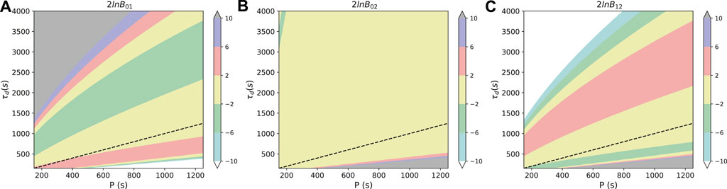
FIGURE 6. Bayes factors in the one-to-one comparison between resonant absorption, phase mixing, and wave leakage mechanisms as a function of the observables period and damping time with uncertainties of 10% for each. The dashed lines indicate τ_d = P. The different levels of evidence are indicated in the colour bars. Not Worth a bare mention (NWM, yellow), Positive (PE, green/red), Strong (SE, blue/purple), Very strong (VSE, white/grey). Adapted from Montes-Solís and Arregui (2017).

The results discussed so far were obtained by application of Bayesian model comparison methods to synthetic hypothetical data in the plane of observables of period and damping time. Montes-Solís and Arregui (2017) also considered the computation of Bayes factors for a selection of 89 loop oscillation events listed in the databases by Verwichte et al. (2013) and Goddard et al. (2016). The results are displayed in Figure 7. The colours indicate the level of evidence, based on the magnitude of the corresponding Bayes factor. It is clear that the events in blue colour, which correspond to evidence that is not worth a bare mention, dominate in all three panels. In the comparison between resonant absorption and phase mixing (left panel), in approximately 78% of the events the evidence is not strong enough to favour one model or the other. The evidence is positive for resonant absorption in 8% of the events and for phase mixing in about 14% of the events. In the middle panel, the comparison between resonant absorption and wave leakage is shown. The evidence is not large enough to support any of the two mechanisms. The panel in the right shows the evidence assessment between phase mixing and wave leakage. In this case, the evidence is inconclusive for 79% of the events. There is positive evidence in favour of wave leakage in 3% of the events, those corresponding to oscillations with very strong damping. For the remaining 18%, the evidence is positive in favour of phase mixing.

FIGURE 7

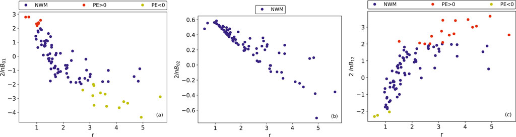
FIGURE 7. Representation of the Bayes factors computed for the 89 events selected from Verwichte et al. (2013) and Goddard et al. (2016). The different panels correspond to the three one-to-one comparisons between resonant absorption, phase mixing, and wave leakage, here represented with the subscripts 0, 1, and 2 respectively. Adapted from Montes-Solís and Arregui (2017).

The results presented by Montes-Solís and Arregui (2017) do not allow us to identify a unique mechanism as responsible for the quick damping of coronal loop oscillations. However, the method makes use of all the available information in the models, observed data with their uncertainty, and prior information in a consistent manner.

3.4 Evidence for Resonant Damping of Coronal Waves With Foot-point Wave Power Asymmetry

Waves propagating in extended regions of the solar corona offer another opportunity to test our models for the damping of waves and oscillations. Their existence was first demonstrated by Tomczyk et al. (2007) and, although first interpreted as Alfvén waves, theoretical arguments by Goossens et al. (2012) showed that an interpretation in terms of kink waves damped by resonant absorption offers a more accurate description. The observed waves show signatures of in situ wave damping in the form of a discrepancy between the outward and the inward wave power. This led Verth et al. (2010) to produce a theoretical model connecting the average power ratio for inward and outward propagating waves with their damping rate. This expression is

${⟨P\left(f\right)⟩}_{\text{ratio}}=R_0\exp \left(\frac{2L}{v_{\text{ph}}{\xi }_{\text{E}}}f\right),(12)$

with R₀ = P_out(f)/P_in(f) the ratio of powers generated at the two foot-points. The exponential factor contains wave propagation and damping properties: the wave travel time along the full wave path of length L, 2L/v_ph, the frequency f and the damping ratio, ξ_E. In the absence of damping, ξ_E → ∞ and ⟨P(f)⟩_ratio = R₀, thus the average power ratio equals the ratio of powers at the two foot-points.

The model by Verth et al. (2010) predicts an exponential dependence of the average power ratio with frequency. A least squares fit to a set of data from the Coronal Multi-channel Polarimeter (CoMP) performed by these authors shows a good qualitative agreement and enabled them to infer a value for the damping ratio ξ_E. However, one must bear in mind that a fitting procedure consists of adopting a model M and obtaining the set of so-called best fit parameters θ. As explained above, Bayesian inference aims at obtaining a solution in terms of a probability distribution of the parameters conditional on the model and on the data, p(θ|M, D). There is no room for absolute statements concerning model evidence because the evidence in favour of a model is always relative to the evidence in favour of another.

Montes-Solís and Arregui (2020) performed a Bayesian analysis to quantify the evidence in favour of resonant damping using CoMP. Instead of considering an alternative damping mechanism the focus was on trying to quantify the evidence in favour of resonant damping in front of the other possible source of discrepancy between the inward and outward power ratio in the corona, namely, an asymmetry in the wave power ratio at the foot-points, i.e., R₀ ≠ 1 in Eq. 12. We note that if P_out(f) > P_in(f), foot-point driving asymmetry will increase the contribution of resonant damping. Conversely, for P_out(f) < P_in(f), the asymmetry will decrease the contribution of resonant damping to the average power ratio.

In their analysis, Montes-Solís and Arregui (2020) first consider the inference of the two parameters of interest, ξ_E and R₀, from a set of CoMP data points for average power ratio as a function of frequency in the range 0.05–4 mHz. The resulting marginal posteriors are shown in Figure 8. The set of CoMP observations is equally well explained by a reduced model, M_R, with parameter distribution p(ξ_E|M_R, D) that considers resonant damping as the sole contributor to the average power ratio and by the larger model, M_A, with parameter distributions p(ξ_E|M_A, D) and p(R₀|M_A, D), which additionally considers foot-point asymmetry. The full posterior for R₀ is within the region below one. This means that P_out < P_in and there is asymmetry in the power generated at both foot-points. The corresponding inference for ξ_E is shifted towards the region corresponding to stronger damping (smaller values of ξ_E) to counterbalance the decreasing factor due to the asymmetry at the foot-points.

FIGURE 8

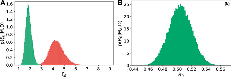
FIGURE 8. (A) Marginal posterior distributions for ξ_E conditional on data D and models M_R (red) and M_A (green). (B) Marginal posterior distribution for R₀ conditional on data D and model M_A. The data D consist of the collective use of the CoMP data set analysed by Verth et al. (2010). The posterior summaries are ${\widehat{\xi }}_{\text{E}}^{\text{MAP}}=4.3_{-0.6}^{+0.7}$ for p(ξ_E|M_R, D), ${\widehat{\xi }}_{\text{E}}^{\text{MAP}}=1.9_{-0.2}^{+0.3}$ for p(ξ_E|M_A, d), and ${\widehat{R}}_0^{\text{MAP}}=0.5\pm 0.02$ for p(R₀|M_A, D), with uncertainty given at the 68% credible interval. The posteriors are computed by Markov Chain Monte Carlo (MCMC) sampling using the Python emcee package (Foreman-Mackey et al., 2013). Adapted from Montes-Solís and Arregui (2020).

Observations can therefore be equally well explained by two models, with or without foot-point asymmetry. To quantify the relative merit of the two explanations, Montes-Solís and Arregui (2020) perform model comparison using the Bayes factor

$B_{\text{RA}}=\frac{p\left(\mathcal{D}|M_{\text{R}}\right)}{p\left(\mathcal{D}|M_{\text{A}}\right)}.(13)$

The Bayes factor is computed in the two-dimensional plane of synthetic data $\mathcal{D}$, covering the full ranges in frequency and average power ratio of CoMP observations, $\mathcal{D}=(f,{⟨P(f)⟩}_{\text{ratio}})$. To this end, Eq. 12 is used to generate theoretical predictions over a grid of points in f and ⟨P(f)⟩_ratio.

Figure 9 shows the distribution of Bayes factor values over the two-dimensional synthetic data space. It is clear that the evidence distribution is inhomogeneous and three different regions, can be identified. They are delimited by the boundaries where the marginal likelihoods are equal and therefore the Bayes factor is zero. In the central region, within the solid boundary lines, model M_R is in principle more plausible than model M_A, because the marginal likelihood for this model is larger. The level of relative plausibility depends on the Bayes factor value, B_RA. In the white area, the evidence in favour of M_R is inconclusive and then varies from positive to very strong in the blue to green areas. Above and below the solid lines, model M_A is more plausible, because the marginal likelihood for this model is larger. However, based on the numerical value for the Bayes factor B_AR, the evidence is inconclusive in the white areas and varies from positive to very strong as we move further towards the upper and lower areas in the plane of observables.

FIGURE 9

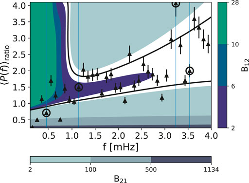
FIGURE 9. Filled contour with the distribution of Bayes factors, B_RA and B_AR, over the two-dimensional data space $\mathcal{D}$. Solid lines connect points with $p(\mathcal{D}|M_{\text{R}})=p(\mathcal{D}|M_{\text{A}})$ (Bayes factor zero). The computations are performed over a grid of points (N_f = 80, $N_{{⟨P(f)⟩}_{\text{ratio}}}$ = 155) over the ranges f ∈ [0.05, 4] and ⟨P(f)⟩_ratio ∈ [0.25, 4.1]. The priors are $p({\xi }_{\text{E}})\sim \mathcal{G}(1.9,0.3)$ for M_R and $p({\xi }_{\text{E}})\sim \mathcal{G}(4.3,0.6)$; $p(R_0)\sim \mathcal{G}(0.5,0.02)$ for M_A. Triangles represent CoMP data. Following Kass and Raftery (1995), the evidence in favour of a model i in front of an alternative j is inconclusive for values of 2log(B_ij) from 0 to 2; positive from 2 to 6; strong from 6 to 10; and very strong for values above 10. Adapted from Montes-Solís and Arregui (2020).

Superimposed over the distribution of Bayes factors in Figure 9 are observed CoMP data with assumed error bars. We can see that in most of the cases, data fall over regions where the marginal likelihood for model M_R is larger. A fraction of them are located over areas where the evidence in favour of model M_R is conclusive. Interestingly, some of them fall into the two regions where the marginal likelihood for model M_A is larger. In some cases, they are over areas where the evidence supports model M_A in front of model M_R.

These results indicate that CoMP measurements of integrated average power ratio for propagating coronal waves cannot exclude an explanation in terms of asymmetry in the wave power generated at the foot-points. Some observations are equally or even better explained by larger models with foot-point wave power asymmetry than by the reduced models with identical power at the two foot-points and resonant damping as the only contributor to the observed average power ratio.

3.5 Evidence for a Nonlinear Damping Model for Waves in the Corona

Recent observational and theoretical studies have shown that the damping of transverse loop oscillations depends on the oscillation amplitude (Goddard et al., 2016; Magyar and Van Doorsselaere, 2016). The increase in the number and quality of observations has led to the creation of catalogs with a large number of events (Anfinogentov et al., 2015; Goddard et al., 2016; Nechaeva et al., 2019; Tiwari et al., 2021). When the damping time over the period is plotted against the oscillation amplitude, the data are scattered forming a cloud with a triangular shape (see e.g., Figure 6 in Nechaeva et al., 2019). In general, larger amplitudes correspond to smaller damping ratio values and vice versa. In a recent study, Arregui (2021) considered the mechanisms of linear resonant absorption, in the formulation given by Ruderman and Roberts (2002) and Goossens et al. (2002) and of nonlinear damping, in the formulation given by Van Doorsselaere et al. (2021). Their analytical developments provide us with two analytical expressions for the damping ratio in cylindrically symmetric waveguides.

For linear resonant absorption, model M_RA, the damping ratio is given by

$\frac{{\tau }_{\text{d}}}{P}{\Vert }_{M_{\text{RA}}}=\mathcal{F}\frac{\zeta +1}{\zeta -1}\frac{R}{l},(14)$

with ζ = ρ_i/ρ_e the ratio of internal to external density, l/R the length of the non-uniform layer at the boundary of the waveguide with radius R, and $\mathcal{F}=2/\pi$ for a sinusoidal variation of density over the non-uniform layer. The predictions from the damping model M_RA given by Eq. 14 for the observable damping ratio are determined by the parameter vector θ_RA = {ζ, l/R}.

For the nonlinear damping of standing kink waves, due to the energy transfer to small scales in the radial and azimuthal directions, the damping ratio is given by

$\frac{{\tau }_{\text{d}}}{P}{\Vert }_{M_{\text{NL}}}=40\sqrt{\pi }\frac{1}{2\pi a}\frac{1+\zeta }{\sqrt{{\zeta }^2-2\zeta +97}},(15)$

with a = η/R the ratio of the displacement η to the loop radius. The predictions from the damping model M_NL given by Eq. 15 for the observable damping ratio, for known oscillation amplitude, are determined by the parameter vector θ_NL = {R, ζ}.

Theoretical predictions from these two models can be confronted by computing the marginal likelihood of the data in the plane of observables defined by the damping ratio and the oscillation amplitude, $\mathcal{D}=\{\eta ,{\tau }_{\text{d}}/P\}$. The ratio of marginal likelihoods leads to the Bayes factor distributions over $\mathcal{D}$-space shown in Figure 10. The two panels show that there is a clear separation between the regions over synthetic data space over which evidence in favour of one or the other model dominates. The evidence supports the nonlinear damping model in a particular region corresponding to combinations with small amplitude and large damping ratio values in the upper-left region of the plane and extending towards the lower-right region corresponding to combinations with smaller damping ratio and larger oscillation amplitude values in a broader range. On the other hand, the evidence supports resonant damping in two regions. The first one extends towards the right-hand side of the domain. The second consists of a small region corresponding to combinations of very small amplitude and strong damping. Overall, the observed data fall within the regions with the largest Bayes factor values for the nonlinear damping model.

FIGURE 10

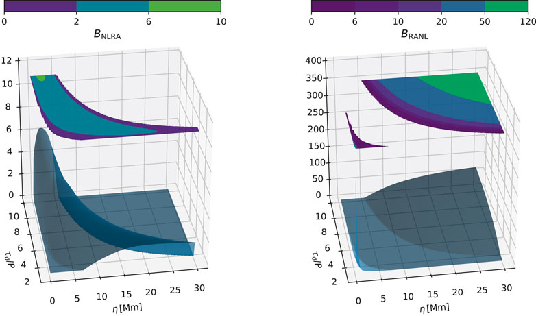
FIGURE 10. Surface and filled contour representations of the Bayes factors B_NLRA (left panel) and B_RANL (right panel) in the synthetic data space $\mathcal{D}=(\eta ,{\tau }_{\text{d}}/P)$. The Bayes factors were computed using the marginal likelihood calculations for each model. Adapted from Arregui (2021).

The analysis using synthetic data over prescribed ranges for the observable amplitude and damping ratio offers a birds-eye view of the distribution of the evidence. The application to observed data offers a better informed result on the level of evidence for or against each damping model. The catalog by Nechaeva et al. (2019) contains 223 loop oscillating loops observed with SDO/AIA in the period 2010–2018. In 101 cases, they contain information about the damping and the oscillation amplitude. Arregui (2021) applied a Bayesian evidence analysis to these data to assess the strength of the evidence for nonlinear damping relative to that for resonant absorption.

Figure 11 displays the results obtained for all 101 cases, regardless of the conclusive or inconclusive nature of the evidence. The red colour indicates evidence in favour of nonlinear damping. The full red dots indicate positive evidence. The edge coloured circles are cases with marginal likelihood for nonlinear damping larger than the marginal likelihood for resonant damping, but inconclusive evidence because the Bayes factor is below 2. The blue colour indicates evidence in favour of resonant damping. The full blue dots indicate positive evidence. The edge coloured circles are cases with marginal likelihood for resonant damping larger than the marginal likelihood for nonlinear damping, but inconclusive evidence because the Bayes factor is below 2. The marginal likelihood in favour of nonlinear damping is larger in the majority of cases. The events with conclusive evidence for nonlinear damping largely outnumber those in favour of linear resonant absorption. The evidence for the nonlinear damping model relative to linear resonant absorption is therefore appreciable to a reasonable degree of Bayesian certainty.

FIGURE 11

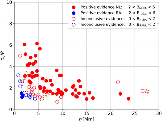
FIGURE 11. Scatter plot of the 101 loop oscillation events in the Nechaeva et al. (2019) catalog with information about both the oscillation amplitude and the damping ratio. In the Bayesian evidence analysis by Arregui (2021), colour filled circles represent cases with conclusive evidence. Edge coloured circles represent cases with either $p(\mathcal{D}|M_{\text{NL}})>p(\mathcal{D}|M_{\text{RA}})$ or vice versa, yet inconclusive evidence. Red is for M_NL and blue for M_RA. Adapted from Arregui (2021).

4 Summary

Bayesian analysis tools are increasingly being used in seismology of the solar corona. In parameter inference, they led to the inference of relevant information on the structure of coronal loops or prominence plasmas, such as the magnetic field strength or the plasma density. Model comparison techniques have been used to assess the damping mechanism operating in coronal loop oscillations. In a comparison between a particular linear and a particular nonlinear damping mechanism, the latter seems to be more plausible in explaining observations. Note that we might have left out important alternative physical processes that could be more plausible instead. This could be assessed by performing additional one-to-one comparisons. Because of our inability to directly measure the physical conditions in the structures of interest, the Bayesian approach offers the best solution to inference problems under uncertain and incomplete information. It uses principled ways to combine the information from data, theoretical models and previous knowledge. The grow in the number of dedicated computing tools to sample multidimensional posterior and marginal likelihood spaces will enable us to apply these methods to additional phenomena related to the structure, dynamics and heating of the solar atmosphere.

Author Contributions

The author confirms being the sole contributor of this work and has approved it for publication.

Funding

Funding provided under project PGC2018-102108-B-I00 from Ministerio de Ciencia, Innovación y Universidades (Spain) and FEDER funds.

Conflict of Interest

The author declares that the research was conducted in the absence of any commercial or financial relationships that could be construed as a potential conflict of interest.

Publisher’s Note

All claims expressed in this article are solely those of the authors and do not necessarily represent those of their affiliated organizations, or those of the publisher, the editors and the reviewers. Any product that may be evaluated in this article, or claim that may be made by its manufacturer, is not guaranteed or endorsed by the publisher.

Acknowledgments

I am grateful to Andrés Asensio Ramos, Marcel Goossens, and María Montes-Solís for years of fruitful collaboration. Calculations and figures were implemented with numpy (Harris et al., 2020) and matplotlib (Hunter, 2007). This research has made use of NASA’s Astrophysics Data System Bibliographic Services.

References

Anfinogentov, S. A., Antolin, P., Inglis, A. R., Kolotkov, D., Kupriyanova, E. G., McLaughlin, J. A., et al. (2021a). Novel Data Analysis Techniques in Coronal Seismology. arXiv e-prints. arXiv:2112.13577.

Google Scholar

Anfinogentov, S. A., Nakariakov, V. M., and Nisticò, G. (2015). Decayless Low-Amplitude Kink Oscillations: a Common Phenomenon in the Solar corona? Astron. Astrophysics 583, A136. doi:10.1051/0004-6361/201526195

CrossRef Full Text | Google Scholar

Anfinogentov, S. A., Nakariakov, V. M., Pascoe, D. J., and Goddard, C. R. (2021b). Solar Bayesian Analysis Toolkit-A New Markov Chain Monte Carlo IDL Code for Bayesian Parameter Inference. ApJS 252, 11. doi:10.3847/1538-4365/abc5c1

CrossRef Full Text | Google Scholar

Arregui, I., and Asensio Ramos, A. (2011). Bayesian Magnetohydrodynamic Seismology of Coronal Loops. Astrophysical J. 740, 44. doi:10.1088/0004-637x/740/1/44

CrossRef Full Text | Google Scholar

Arregui, I., and Asensio Ramos, A. (2014). Determination of the Cross-Field Density Structuring in Coronal Waveguides Using the Damping of Transverse Waves. Astron. Astrophysics 565, A78. doi:10.1051/0004-6361/201423536

CrossRef Full Text | Google Scholar

Arregui, I., Asensio Ramos, A., and Díaz, A. J. (2013a). Bayesian Analysis of Multiple Harmonic Oscillations in the Solar Corona. Astrophysical J. 765, L23. doi:10.1088/2041-8205/765/1/l23

CrossRef Full Text | Google Scholar

Arregui, I., Asensio Ramos, A., and Pascoe, D. J. (2013b). Determination of Transverse Density Structuring from Propagating Magnetohydrodynamic Waves in the Solar Atmosphere. Astrophysical J. 769, L34. doi:10.1088/2041-8205/769/2/l34

CrossRef Full Text | Google Scholar

Arregui, I., Ballester, J. L., and Goossens, M. (2008). On the Scaling of the Damping Time for Resonantly Damped Oscillations in Coronal Loops. Astrophysical J. 676, L77–L80. doi:10.1086/587098

CrossRef Full Text | Google Scholar

Arregui, I. (2018). Bayesian Coronal Seismology. Adv. Space Res. 61, 655–672. doi:10.1016/j.asr.2017.09.031

CrossRef Full Text | Google Scholar

Arregui, I. (2021). Bayesian Evidence for a Nonlinear Damping Model for Coronal Loop Oscillations. ApJL 915, L25. doi:10.3847/2041-8213/ac0d53

CrossRef Full Text | Google Scholar

Arregui, I., and Goossens, M. (2019). No Unique Solution to the Seismological Problem of Standing Kink Magnetohydrodynamic Waves. Astron. Astrophysics 622, A44. doi:10.1051/0004-6361/201833813

CrossRef Full Text | Google Scholar

Arregui, I., Montes-Solís, M., and Asensio Ramos, A. (2019). Inference of Magnetic Field Strength and Density from Damped Transverse Coronal Waves. Astron. Astrophysics 625, A35. doi:10.1051/0004-6361/201834324

CrossRef Full Text | Google Scholar

Arregui, I., Soler, R., and Asensio Ramos, A. (2015). Model Comparison for the Density Structure across Solar Coronal Waveguides. Astrophysical J. 811, 104. doi:10.1088/0004-637X/811/2/104

CrossRef Full Text | Google Scholar

Arregui, I., and Soler, R. (2015). Model Comparison for the Density Structure along Solar Prominence Threads. Astron. Astrophysics 578, A130. doi:10.1051/0004-6361/201525720

CrossRef Full Text | Google Scholar

Arregui, I. (2015). Wave Heating of the Solar Atmosphere. Phil. Trans. R. Soc. A. 373, 20140261. doi:10.1098/rsta.2014.0261

PubMed Abstract | CrossRef Full Text | Google Scholar

Aschwanden, M. J., Fletcher, L., Schrijver, C. J., and Alexander, D. (1999). Coronal Loop Oscillations Observed with theTransition Region and Coronal Explorer. Astrophysical J. 520, 880–894. doi:10.1086/307502

CrossRef Full Text | Google Scholar

Asensio Ramos, A., and Arregui, I. (2013). Coronal Loop Physical Parameters from the Analysis of Multiple Observed Transverse Oscillations. Astron. Astrophysics 554, A7. doi:10.1051/0004-6361/201321428

CrossRef Full Text | Google Scholar

Asensio Ramos, A., Martínez González, M. J., and Rubiño-Martín, J. A. (2007). Bayesian Inversion of Stokes Profiles. Astron. Astrophysics 476, 959–970. doi:10.1051/0004-6361:20078107

CrossRef Full Text | Google Scholar

Bayes, M., and Price, M. (1763). An Essay towards Solving a Problem in the Doctrine of Chances. By the Late Rev. Mr. Bayes, F. R. S. Communicated by Mr. Price, in a Letter to John Canton, A. M. F. R. S. R. Soc. Lond. Philos. Trans. Ser. 53, 370–418.

Google Scholar

Cally, P. S. (2003). Coronal Leaky Tube Waves and Oscillations Observed with Trace. Solar Phys. 217, 95–108. doi:10.1023/A:1027326916984

CrossRef Full Text | Google Scholar

De Pontieu, B., Martens, P. C. H., and Hudson, H. S. (2001). Chromospheric Damping of Alfven Waves. Astrophysical J. 558, 859–871. doi:10.1086/322408

CrossRef Full Text | Google Scholar

Duckenfield, T. J., Goddard, C. R., Pascoe, D. J., and Nakariakov, V. M. (2019). Observational Signatures of the Third Harmonic in a Decaying Kink Oscillation of a Coronal Loop. Astron. Astrophysics 632, A64. doi:10.1051/0004-6361/201936822

CrossRef Full Text | Google Scholar

Foreman-Mackey, D., Hogg, D. W., Lang, D., and Goodman, J. (2013). Emcee: The MCMC Hammer. Publications Astronomical Soc. Pac. 125, 306–312. doi:10.1086/670067

CrossRef Full Text | Google Scholar

Gates, E., Krauss, L. M., and White, M. (1995). Treating Solar Model Uncertainties: A Consistent Statistical Analysis of Solar Neutrino Models and Data. Phys. Rev. D 51, 2631–2643. doi:10.1103/PhysRevD.51.2631

PubMed Abstract | CrossRef Full Text | Google Scholar

Goddard, C. R., Antolin, P., and Pascoe, D. J. (2018). Evolution of the Transverse Density Structure of Oscillating Coronal Loops Inferred by Forward Modeling of EUV Intensity. Astrophysical J. 863, 167. doi:10.3847/1538-4357/aad3cc

CrossRef Full Text | Google Scholar

Goddard, C. R., Nisticò, G., Nakariakov, V. M., and Zimovets, I. V. (2016). A Statistical Study of Decaying Kink Oscillations Detected Using SDO/AIA. Astron. Astrophysics 585, A137. doi:10.1051/0004-6361/201527341

CrossRef Full Text | Google Scholar

Goddard, C. R., Pascoe, D. J., Anfinogentov, S., and Nakariakov, V. M. (2017). A Statistical Study of the Inferred Transverse Density Profile of Coronal Loop Threads Observed with Sdo/aia. Astron. Astrophysics 605, A65. doi:10.1051/0004-6361/201731023

CrossRef Full Text | Google Scholar

Goossens, M., Andries, J., and Arregui, I. (2006). Damping of Magnetohydrodynamic Waves by Resonant Absorption in the Solar Atmosphere. Phil. Trans. R. Soc. A. 364, 433–446. doi:10.1098/rsta.2005.1708

PubMed Abstract | CrossRef Full Text | Google Scholar

Goossens, M., Andries, J., and Aschwanden, M. J. (2002). Coronal Loop Oscillations. Astron. Astrophysics 394, L39–L42. doi:10.1051/0004-6361:20021378

CrossRef Full Text | Google Scholar

Goossens, M., Andries, J., Soler, R., Van Doorsselaere, T., Arregui, I., and Terradas, J. (2012). Surface Alfvén Waves in Solar Flux Tubes. Astrophysical J. 753, 111. doi:10.1088/0004-637X/753/2/111

CrossRef Full Text | Google Scholar

Harris, C. R., Millman, K. J., van der Walt, S. J., Gommers, R., Virtanen, P., Cournapeau, D., et al. (2020). Array Programming with NumPy. Nature 585, 357–362. doi:10.1038/s41586-020-2649-2

PubMed Abstract | CrossRef Full Text | Google Scholar

Heyvaerts, J., and Priest, E. R. (1983). Coronal Heating by Phase-Mixed Shear Alfven Waves. Astron. Astrophys. 117, 220.

Google Scholar

Hunter, J. D. (2007). Matplotlib: A 2d Graphics Environment. Comput. Sci. Eng. 9, 90–95. doi:10.1109/MCSE.2007.55

CrossRef Full Text | Google Scholar

Kass, R. E., and Raftery, A. E. (1995). Bayes Factors. J. Am. Stat. Assoc. 90, 773–795. doi:10.1080/01621459.1995.10476572

CrossRef Full Text | Google Scholar

Lin, Y., Soler, R., Engvold, O., Ballester, J. L., Langangen, Ø., Oliver, R., et al. (2009). Swaying Threads of a Solar Filament. Astrophysical J. 704, 870–876. doi:10.1088/0004-637x/704/1/870

CrossRef Full Text | Google Scholar

Magyar, N., and Van Doorsselaere, T. (2016). Damping of Nonlinear Standing Kink Oscillations: a Numerical Study. Astron. Astrophysics 595, A81. doi:10.1051/0004-6361/201629010

CrossRef Full Text | Google Scholar

Marsh, M. S., Ireland, J., and Kucera, T. (2008). Bayesian Analysis of Solar Oscillations. Astrophysical J. 681, 672–679. doi:10.1086/588751

CrossRef Full Text | Google Scholar

Montes-Solís, M., and Arregui, I. (2017). Comparison of Damping Mechanisms for Transverse Waves in Solar Coronal Loops. Astrophysical J. 846, 89. doi:10.3847/1538-4357/aa84b7

CrossRef Full Text | Google Scholar

Montes-Solís, M., and Arregui, I. (2019). Inferring Physical Parameters in Solar Prominence Threads. Astron. Astrophysics 622, A88. doi:10.1051/0004-6361/201834406

CrossRef Full Text | Google Scholar

Montes-Solís, M., and Arregui, I. (2020). Quantifying the Evidence for Resonant Damping of Coronal Waves with Foot-point Wave Power Asymmetry. Astron. Astrophysics 640, L17. doi:10.1051/0004-6361/201937237

CrossRef Full Text | Google Scholar

Nakariakov, V. M., Ofman, L., DeLuca, E. E., Roberts, B., and Davila, J. M. (1999). TRACE Observation of Damped Coronal Loop Oscillations: Implications for Coronal Heating. Science 285, 862–864. doi:10.1126/science.285.5429.862

PubMed Abstract | CrossRef Full Text | Google Scholar

Nakariakov, V. M., and Ofman, L. (2001). Determination of the Coronal Magnetic Field by Coronal Loop Oscillations. Astron. Astrophysics 372, L53–L56. doi:10.1051/0004-6361:20010607

CrossRef Full Text | Google Scholar

Nechaeva, A., Zimovets, I. V., Nakariakov, V. M., and Goddard, C. R. (2019). Catalog of Decaying Kink Oscillations of Coronal Loops in the 24th Solar Cycle. ApJS 241, 31. doi:10.3847/1538-4365/ab0e86

CrossRef Full Text | Google Scholar

Ofman, L., and Aschwanden, M. J. (2002). Damping Time Scaling of Coronal Loop Oscillations Deduced from [ITAL]Transition Region and Coronal Explorer[/ITAL] Observations. Astrophys. J. Lett. 576, L153–L156. doi:10.1086/343886

CrossRef Full Text | Google Scholar

Pascoe, D. J., Anfinogentov, S. A., Goddard, C. R., and Nakariakov, V. M. (2018). Spatiotemporal Analysis of Coronal Loops Using Seismology of Damped Kink Oscillations and Forward Modeling of EUV Intensity Profiles. Astrophysical J. 860, 31. doi:10.3847/1538-4357/aac2bc

CrossRef Full Text | Google Scholar

Pascoe, D. J., Anfinogentov, S., Nisticò, G., Goddard, C. R., and Nakariakov, V. M. (2017a). Coronal Loop Seismology Using Damping of Standing Kink Oscillations by Mode Coupling. Astron. Astrophysics 600, A78. doi:10.1051/0004-6361/201629702

CrossRef Full Text | Google Scholar

Pascoe, D. J., Goddard, C. R., Anfinogentov, S., and Nakariakov, V. M. (2017b). Coronal Loop Density Profile Estimated by Forward Modelling of EUV Intensity. Astron. Astrophysics 600, L7. doi:10.1051/0004-6361/201730458

CrossRef Full Text | Google Scholar

Pascoe, D. J., Goddard, C. R., and Van Doorsselaere, T. (2020a). Oscillation and Evolution of Coronal Loops in a Dynamical Solar corona. Front. Astron. Space Sci. 7, 61. doi:10.3389/fspas.2020.00061

CrossRef Full Text | Google Scholar

Pascoe, D. J., Hood, A. W., and Van Doorsselaere, T. (2019). Coronal Loop Seismology Using Standing Kink Oscillations with a Lookup Table. Front. Astron. Space Sci. 6, 22. doi:10.3389/fspas.2019.00022

CrossRef Full Text | Google Scholar

Pascoe, D. J., Russell, A. J. B., Anfinogentov, S. A., Simões, P. J. A., Goddard, C. R., Nakariakov, V. M., et al. (2017c). Seismology of Contracting and Expanding Coronal Loops Using Damping of Kink Oscillations by Mode Coupling. Astron. Astrophysics 607, A8. doi:10.1051/0004-6361/201730915

CrossRef Full Text | Google Scholar

Pascoe, D. J., Smyrli, A., and Van Doorsselaere, T. (2020b). Tracking and Seismological Analysis of Multiple Coronal Loops in an Active Region. Astrophysical J. 898, 126. doi:10.3847/1538-4357/aba0a6

CrossRef Full Text | Google Scholar

Richardson, W. H. (1972). Bayesian-Based Iterative Method of Image Restoration*. J. Opt. Soc. Am. 62, 55. doi:10.1364/josa.62.000055

CrossRef Full Text | Google Scholar

Roberts, B., Edwin, P. M., and Benz, A. O. (1984). On Coronal Oscillations. Astrophysical J. 279, 857. doi:10.1086/161956

CrossRef Full Text | Google Scholar

Roberts, B. (2000). Waves and Oscillations in the corona - (Invited Review). Solar Phys. 193, 139–152. doi:10.1023/a:1005237109398

CrossRef Full Text | Google Scholar

Ruderman, M. S., and Roberts, B. (2002). The Damping of Coronal Loop Oscillations. Astrophysical J. 577, 475–486. doi:10.1086/342130

CrossRef Full Text | Google Scholar

Soler, R., Arregui, I., Oliver, R., and Ballester, J. L. (2010). Seismology of Standing Kink Oscillations of Solar Prominence fine Structures. Astrophysical J. 722, 1778–1792. doi:10.1088/0004-637x/722/2/1778

CrossRef Full Text | Google Scholar

Soler, R., and Goossens, M. (2011). Kink Oscillations of Flowing Threads in Solar Prominences. Astron. Astrophysics 531, A167. doi:10.1051/0004-6361/201116536

CrossRef Full Text | Google Scholar

Spruit, H. C. (1982). Propagation Speeds and Acoustic Damping of Waves in Magnetic Flux Tubes. Sol. Phys. 75, 3–17. doi:10.1007/BF00153456

CrossRef Full Text | Google Scholar

Sturrock, P. A. (1973). Evaluation of Astrophysical Hypotheses. Astrophysical J. 182, 569–580. doi:10.1086/152165

CrossRef Full Text | Google Scholar

Tiwari, A. K., Morton, R. J., and McLaughlin, J. A. (2021). A Statistical Study of Propagating MHD Kink Waves in the Quiescent Corona. Astrophysical J. 919, 74. doi:10.3847/1538-4357/ac10c4

CrossRef Full Text | Google Scholar

Tomczyk, S., McIntosh, S. W., Keil, S. L., Judge, P. G., Schad, T., Seeley, D. H., et al. (2007). Alfvén Waves in the Solar Corona. Science 317, 1192–1196. doi:10.1126/science.1143304

PubMed Abstract | CrossRef Full Text | Google Scholar

Uchida, Y. (1970). Diagnosis of Coronal Magnetic Structure by Flare-Associated Hydromagnetic Disturbances. Pub. Astron. Soc. Jpn. 22, 341.

Google Scholar

Van Doorsselaere, T., Goossens, M., Magyar, N., Ruderman, M. S., and Ismayilli, R. (2021). Nonlinear Damping of Standing Kink Waves Computed with Elsässer Variables. Astrophysical J. 910, 58. doi:10.3847/1538-4357/abe630

CrossRef Full Text | Google Scholar

Verth, G., Terradas, J., and Goossens, M. (2010). Observational Evidence of Resonantly Damped Propagating Kink Waves in the Solar Corona. Astrophysical J. 718, L102–L105. doi:10.1088/2041-8205/718/2/L102

CrossRef Full Text | Google Scholar

Verwichte, E., Van Doorsselaere, T., White, R. S., and Antolin, P. (2013). Statistical Seismology of Transverse Waves in the Solar corona. Astron. Astrophysics 552, A138. doi:10.1051/0004-6361/201220456

CrossRef Full Text | Google Scholar

Wheatland, M. S. (2004). A Bayesian Approach to Solar Flare Prediction. Astrophysical J. 609, 1134–1139. doi:10.1086/421261

CrossRef Full Text | Google Scholar