Jovian Planets and Lunar Nodal Cycles in the Earth’s Climate Variability

Introduction

Studies using climate models have observed global multidecadal variation originating from an unknown source (Mann et al., 2020). Kravtsov et al. (2018) found that current climate models fail to explain a substantial amount of global climate variation. The unexplained variation can be up to 0.3°C. Multidecadal temperature variations on Earth may be deterministic or random; deterministic variations originating from known sources can be used to predict future variations, whereas random (nondeterministic) variations originating from unknown sources can only explain past events. Stationary cycles in time series are deterministic if the cycles have deterministic external sources. Deterministic variation from an external source may serve as a reference for climate variation. Some possible external sources of deterministic stationary climate cycles include stationary cycles in total solar irradiance (TSI) cycles, originating from planet cycles, and stationary lunar-forced temperature variations, originating from the Earth’s axis nutation. When phase relations between the stationary cycles are known, it opens new possibilities for estimating past and future events.

Records have shown correlation between solar variations and global temperatures (Suess 1980). Cycles featuring solar variations, as identified from Greenland ice cores, have stimulated a discussion about the possible planetary modulation of solar irradiation in the solar system. Jose (1965) identified a correlation among planets, i.e., solar barycenter motion with a 179-year cycle. Zhenqiu and Zhisen (1980) analyzed planetary conjunctions and climate in China and estimated minimum temperatures for the years 1982, 2163 and 2344 A.D. Numerous other investigations have elucidated the relationships among planetary cycles, solar irradiance, and climate variations (Fairbridge and Sanders, 1987; Hoyt and Schatten 1993; Satterley, A. K. 1996; Charvátová 2000; Liu et al., 2011; Abreu et al., 2012; Scafetta 2012, 2016; McCracken et al., 2014; Scafetta et al., 2016: Steinhilber and Beer (2013)) studied solar irradiance over a cycle of 9400 years and identified long cycles of 150, 208, 350, 500, 1000, 1450, and 2200 years; the authors also computed a Dalton-type minimum at 2100 A.D. Wavelet spectrum analyses of time series of the TSI, sunspots and solar position have revealed close relations among the TSI variation, solar position oscillation and elliptical orbits of the Jovian planets (Jupiter, Saturn, Uranus, and Neptune) (Yndestad and Solheim 2017).

The oscillation of gravitational forces within the Earth-Moon-Sun system introduces a spectrum of tides that influence the redistribution of heat in the large-scale oceanic thermohaline system. Tidal forcing in the ocean’s thermohaline system introduces vertical temperature mixing in the oceans, which influences sea surface temperatures and atmospheric climate. Studies have revealed that approximately 1 TW (25–30%) of the total dissipation of energy occurs in the deep oceans (Egbert and Ray 2000). The estimated mixing energy required to maintain large-scale thermohaline circulation is approximately 2 TW. Therefore, half of this amount could be provided by tides. The relationship between the temperature variations of the Atlantic Ocean and lunar tides has been discussed for decades. In 1907, Otto Pettersson studied the relationship between herring catches and tides along the west coast of Sweden and concluded that the long-cycle (18- and 111-year) tidal cycles of climate variations were caused by vertical mixing (Pettersson 1905, 1914, 1915). Russian scientists Maksimov and Smirnov (1964, 1967) and Currie (1981) identified an 18.6-year lunar nodal tide as a standing tide between the Earth’s poles and equator. Since the 1960 s, several studies have confirmed the 18.6-year cycle through spectrum analyses (Keeling and Whorf 1997; Gratiot et al., 2008; Hansen et al., 2015; Gustavo et al., 2018). Wavelet spectrum analyses of the water inflows from the North Atlantic into the Norwegian Sea and Barents Sea have identified that this 18.6-year lunar nodal tide introduces surface temperature cycles of 18.6/2, 18.6, 3*18.6 and 4*18.6 years (Yndestad et al., 2008). The same cycles have been identified in the North Atlantic Oscillation (NAO) index, the Arctic Sea ice extent (Yndestad 2021), the Arctic Ocean circulation, and the oscillations of the Earth’s axis (Yndestad 2006). Nevertheless, the cycle- and phase-relations among planetary cycles, TSI variation, lunar-forced ocean temperature variation and global temperature variation are poorly understood. Using known cycle periods and cycle phase relations from Jovian planets and Earth´s axis nutation, this study investigates solar forced temperature variations and lunar forced temperature variations in Earth temperature variation.

Materials and Methods

Theory

This study investigates the relation between cycle periods, cycle phase and cycle amplitude in a chain of events, from the Jovian planets and the Earth’s nutation, to climate variations. Cycle properties and notations are explained in the Nomenclature section.

Jovian Planet Oscillations

The Jovian planets, Jupiter, Saturn, Uranus, and Neptune (JSUN), have elliptic orbital cycles in time-variant distances from the Sun. The elliptic orbital cycles have maximum speeds and minimum distances from the Sun when the orbital phase position is at perihelion and minimum speeds and maximum distances at aphelion. The JSUN elliptic orbital cycles represent an oscillating spectrum, Sjsun (Tjsun, (θjsun (t-t_per)). The Jovian planets have cycle periods (in years) Tjsun = (Tju, Tsa, Tur, Tne) = (11.862, 29.447, 84.02, 164.79) (yr.), and θjsun (t-t_per) represents references to perihelion coincidences. JSUN planets have perihelion position phase coincidences, θjsun (t = t_per), at the year t_per = (t_per-ju, t_per-sa, t_per-ur, t_per-ne) = (1714.69, 1709.00, 1714.32, 1711.88) (yr). (Astronomical Almanac, USNO, Governmental Printing Office). The mean perihelion coincidence occurs in 1712 A.D. JSUN elliptic orbital cycles have aphelion coincidences in the following years: t_aph = ((t_per-ju-187.5Tju), (t_per-sa-75.5Tsa), (t_per-ur -26.5Tur), (t_per-ne-13.5Tne)) = (-509.43, -514.25, -512.21, -512.79) (yr.). The mean aphelion coincidence occurs in 512.17 B.C. The mean envelope time period of JSUN cycle phase coincidences is 4449.28 years. The 4450-year envelope period has phase shifts at Ajsun-en(t) = ((-0, -1624.49), (aper, −512), (+0, 600), (per, 1712), (−0, 2825)).

Solar Position Oscillations

The Sun moves in a closed orbit around the barycenter of the solar system. The solar system oscillation is caused by the mutual gravity dynamics between the planet system oscillation and the solar position oscillation (SPO). The SPO has oscillations in the x, y, and z directions; they are represented by data series SPOx, SPOy, and SPOz, respectively. A wavelet spectrum analysis of SPO time-series in the (x, y, z)-direction revealed a coincidence between JSUN mean perihelion coincidences in 1712 A.D. (Yndestad and Solheim 2017). The coincidence between SPOs and JSUN cycles at the perihelion may be represented as a linear spectrum transform of JSUN cycle periods to SPO oscillations and solar dynamo oscillations. The total solar irradiation spectrum, Stsi, may be represented as a spectrum transformation from JSUN oscillation TSI oscillations.

Total Solar Irradiation Oscillation

Total solar irradiation (TSI) oscillations are represented as a spectrum: Stsi (Ttsi, θtsi (t-t_tsi)), where Ttsi represents TSI cycle periods and θtsi (t = t_tsi) represents the years when TSI periods have a maximum amplitude. TSI amplitude variations, Atsi(t), experience minima when the Jovian planet cycles, Tjsun, experience perihelion coincidences at θjsun (t = t_per) (Yndestad and Solheim 2017). The total solar irradiation spectrum, Stsi (Ttsi, (θtsi (t-t_tsi)), may be computed as a linear spectrum transformation of the JSUN cycle periods into a TSI cycle spectrum by the simplified model:

$\text{Stsi}\left(\text{Ttsi},\mathrm{\theta }\text{tsi}\left(\text{t}-{\text{t}}_{\text{tsi}}\right)\right)=\text{Hsol}\left(\text{Tsol},\text{θsol}\left({\text{t}}_{\text{sol}}\right)\text{Sjsun}\left(\text{Tjsun},\mathrm{\theta }\text{jsun}\left(\text{t}-{\text{t}}_{\text{per}}\right)\right)\right),(1)$

where Hsol (Tsol, θsol (t_sol) represents the Sun´s transformation of JSUN cycles and phase-relation periods into a TSI spectrum Stsi (Ttsi, θtsi (t-t_tsi)). In this transformation, the cycle period transform Tsol = 1 and the phase lag t_sol = 0 (yr.). The transformed spectrum has cycle periods Ttsi = Tsol*Tjsun = Tjsun, and cycle phase shifts θtsi (t_tsi) = θjsun (t_per) + θsol (t_sol) = θjsun (t_per). The 4450-year TSI envelope period has phase shifts in the years: Atsi-en(t) = ((-0, -1624.49), (max, -512), (+0, 600), (min, 1712), (−0, 2825)).

Solar Forced Sea Temperature Oscillations

The solar-forced sea surface temperature (SST) in Earth’s oceans is represented by a spectrum Ssst (Tsst, θsst (t-t_sst)), where Tsst represents the solar-forced SST cycle periods and the phase state, θsst (t_0-sst), represents the years when Tsst cycle periods have amplitude maxima. The accumulation of TSI forced heat cycle periods in Earth’s oceans is expected to have a cycle phase lag of π/2 (rad), or Ttsi/4, from the Sun´s JSUN cycle periods. The solar forced sea temperature spectrum is computed by the simplified model:

$\text{Ssst}\left(\text{Tsst},\text{θsst}\left(\text{t}-{\text{t}}_{\text{sst}}\right)\right)=\text{Hsea}\left(\text{Tsea},\mathrm{\theta }\text{sea}\left({\text{t}}_{\text{sea}}\right)\text{Stsi}\left(\text{Ttso},\mathrm{\theta }\text{tsi}\left(\text{t}-{\text{t}}_{\text{tsi}}\right)\right)\right),(2)$

where Hsea (Tsea, θsea (t_sea) represents the sea surface transformation of TSI cycles and phase-relation periods into an SST spectrum Ssst (Tsst, θsst (t-t_sst)), where Tsol = 1 and t_sea = Tjsun/4. The transformed spectrum has cycle periods Tsst = Tsol^∗Ttsi = Tsol*Tjsun = Tjsun, and cycle phase shifts θsst (t_sst) = θjsun (t_tsi + t_sea) = θjsun (t_per + Tjsun/4). The new 4450-year SST envelope period has phase shifts in the years: Asst-en(t) = ((min, -1624.49), (-0, -512), (max, 600), (-0, 1712), (min, 2825)). Solar-forced SST variations have a maximum speed in the negative direction when solar-forced irradiation has a minimum in 1712.

Lunar Forced Sea Temperature Oscillations

The Earth axis tilt (obliquity of the ecliptic) is approximately 23°27′. Mutual gravity among the Earth-Moon-Sun oscillations introduces a nutation in Earth’s axial tilt and precession. The Earth nutation has amplitude variations of approximately 9.2 s of arc in a cycle period of 18.6134 years. The amplitude variation influences the cross-point between the Moon’s plane cycle and the ecliptic plane to the Sun in a lunar nodal cycle of Tln = 18.61 years. The Earth’s axis nutation spectrum, Sln (Tln, θln (t-t_ln)), has harmonic periods Tln = (1, 2, 3, 4, … )18.61 (yr.) and reached a major standstill maximum in the year t_ln = 1932.3. The nutation spectrum, Sln (Tln, θln (t-t_ln)), introduces a global lunar nodal tide spectrum, Slnt (Tlnt, θlnt (t-t_lnt)), as a standing wave in oceans. The global lunar nodal tide introduces vertical mixing and lunar forced sea surface temperature (LST) variations. The lunar forced sea temperature spectrum is computed by the simplified model:

$\text{Slst}\left(\text{Tlst},\mathrm{\theta }\text{lst}\left(\text{t}-{\text{t}}_{\text{lst}}\right)\right)=\text{Hoce}\left(\text{Toce},\mathrm{\theta }\text{osc}\left({\text{t}}_{\text{oce}}\right)\text{S}\ln \left(\text{T}\ln ,\mathrm{\theta }\ln \left(\text{t}-{\text{t}}_{\text{In}}\right)\right)\right),(3)$

where Hoce(Tose, θoce (t_oce) represents a transformation of Earth’s axis nutation cycles and cycle phase relations into a lunar forced sea surface spectrum Slst (Tlst, θlst (t-t_lst)), where Tose = 1 and t_oce represents the phase lag in oceans. The transformed spectrum has cycle periods of Tlst = Tose*Tln = Tln. The phase lag t_lst = t_ln - t_ose is period dependent and position dependent and must be estimated.

Solar-Lunar-Forced Temperature Oscillations on Earth

The effect of Jovian planets and lunar nodal cycles on the Earth’s climate variation may be represented as a sum of solar lunar forced temperature variations by the simplified model:

$\text{Sslt}=\text{Stsi}+\text{Ssst}+\text{Slst}+\text{Serr},(4)$

where Serr represents a spectrum from an unknown source. The direct solar-forced TSI spectrum, Stsi, the solar-forced sea surface temperature spectrum, Ssst, and the lunar-forced spectrum, Slst, have known cycle periods and cycle phase relations Eqs. 2, 3. The total solar-lunar-forced amplitude variations, Aslt(t) = Atsi(t) + Asst(t) + Alst(t) + Aerr(t), are controlled by constructive and destructive interference between cycle periods and the cycle phase relations.

Materials

This study uses the HadCRUT4 time series, which covers the interval from 1850 to 2020, as a representative proxy of Earth’s global mean temperature. These time series are based on sea surface and land-air temperature estimates (Morice et al., 2012). The sea surface temperature time series (HadSST3) consists of anomalies on a 5°-by-5° global grid, while the land-air temperature time series (CRUTEM4) consists of anomalies on a 5°-by-5° grid and is supported by the Climatic Research Unit (http://www.metoffice.gov.uk/hadobs/hadcrut4/). The Greenland temperatures are represented by the GISP2 time series covering the time periods from 1000 A.D. to 1993 A.D. and from 2000 B.C. to 1993 A.D.; these time series were estimated from nitrogen and argon isotope data extracted from air bubbles in Greenland ice cores at 72°36’N, 38°30’W, 3203 m above sea level. These series are supported by the World Data Center for Paleoclimatology in Boulder, Colorado, United States, and the NOAA Paleoclimatology Program (https://www.ncdc.noaa.gov/data-access/paleoclimatology-data) (Kobashi et al., 2011).

Methods

Cycle periods and cycle phase relations in Earth’s temperature variation are identified in the wavelet spectra of Earth’s temperature time series by the wavelet transform:

$W_{a,b}\left(t\right)=\frac{1}{\sqrt[ ]{a}}{\displaystyle \underset{R}{\int }x\left(t\right)\text{Ψ}\left(\frac{t-b}{a}\right)dt}(5)$

where x(t) is the analyzed temperature time series after being transformed to a zero mean value and scaled by variance. Ψ() is a coif3 wavelet impulse function. $W_{a,b}\left(t\right)$ is a set of wavelet cycles, b is the translation in time, and a is the time-scaling parameter in the wavelet transformation (Daubechies 1992; MATLAB, 2020). In this analysis, the time translation b = 0, and the computed wavelet transformation, $W_a\left(t\right)$, a moving correlation between x(t) and the impulse function Ψ() over the entire time-series x(t). The moving correlated wavelets, s(t), are collected into a wavelet spectrum, W (s, t), for t = (first … last) (yr.) and s = (1 … (last-first)/2) (yr.). A wavelet power spectrum can be defined as:

$WP\left(s, t\right)={\left[W\left(s,t\right)\right]}^2(6)$

In this study, the wavelet power spectrum (Torrence and Compo 1998) estimates the most dominant wavelet amplitude variations. Stationary cycles in the wavelet spectrum, W (s, t), coincide with stationary cycles, T, in the Earth’s temperature spectrum Sest.

Stationary Cycle Periods

Stationary cycles, T, in the Earth’s temperature variability spectrum, Sest(t), are identified by computing the autocorrelation of the wavelet specter W (s, t), as follows:

$\text{W}\left(\text{R}\left(\text{s}\right),\text{m}\right)=\text{E}\left[\text{W}\left(\text{s},\text{t}\right)\text{W}\left(\text{s},\text{t}+\text{m}\right)\right],(7)$

where WR (R, T) represents a set of maximum correlations R = (max 1 … max n) to the stationary cycles T = (T1 … Tn) (yr.).

Source of Stationary Cycles

The effects of Jovian planets and lunar nodal cycles on the Earth’s climate variability are identified by computing the coincidence differences between the estimated spectrum, (S (T, θ(t₀)), from Earth temperature data series and the deterministic solar-lunar forced spectra Stsi (Ttsi, θtsi (t_0-tsi)), Ssst (Tsst, θsst (t_0-sst)) and Slnt (lnt, θlnt (t_0-lnt)).

Results

Total Solar Irradiation Oscillations

The total solar irradiation spectrum, Stsi (Ttsi, (θtsi (t-t_tsi))), may be computed as a linear spectrum transformation of the JSUN cycle periods into a TSI cycle spectrum Eq. 1. The transformed spectrum TSI spectrum has the computed amplitude variations:

$\text{Atsi}\left(\text{jsun},\text{t}\right)={\text{Ktsi}}^{\ast }\cos \left(2\pi \left(\text{t}-{\text{t}}_{\text{tsi}}\right)/\text{Ttsi}\right),(8)$

where Atsi(jsun, t) = (Atsi(ju, t), Atsi(sa, t), Atsi(ur, t), and Atsi(ne, t)) represent TSI amplitude variations from JSUN cycles and the transformed cycle periods Ttsi = Tjsun. TSI cycles have minima when JSUN periods have perihelion phase coincidences for t_tsi = t_per and Kjsun = (Kju, Ksa, Kur, Kne) = (−1, −1, −1, −1). Total amplitude variations are represented by the TSI index Atsi(t) = (Atsi(ju, t) + Atsi(sa, t) + Atsi(ur, t) + Atsi(ne, t)). Atsi(t) has a maximum in 512 B.C. and a minimum in 1712 A.D. The 4450-year TSI envelope period, Atsi-en(t), has phase shifts in the years: Atsi-en(t) = ((−0, −1624.49), (max, −512), (+0, 600), (min, 1712), (−0, 2825)).

The temporary Uranus and Neptune (UN) period coincidences in the envelope period cause temporary TSI minima and maxima. UN cycle periods have the following period coincidences: Tun-co = [(2Tur, Tne), (4Tur, 2Tne), (6Tur, 3Tne), (12Tur, 6Tne), (23Tur, 12Tne), (29Tur, 15Tne), (51Tur, 26Tne), (53Tur, 27Tne)] (yr.), with mean period coincidences of Tun-mco = [166.42, 332.83, 499.70, 998.49, 1954.97, 2454.22, 4284.78, 4451.20] (yr.). Figure 1 shows the computed Eq. 8 amplitude variations, Atsi(un, t) = Atsi(ur, t) + Atsi(ne, t), for the years t = (−2000, … 3000). From 1000 to 3000 A.D. TSI index values, Atsi(nu, t) < −1.90, have a minimum at Atsi(un, t) = ((−1.97, 1212), (−1.98, 1379), (−1.99, 1546), (−2.00, 1713), (−1.98, 1882), (−1.95, 2049), (−1.92, 2216)). “The Little Ice Age” covers five deep minima from 1379 to 2049 and an upcoming computed minimum in 2216.

FIGURE 1

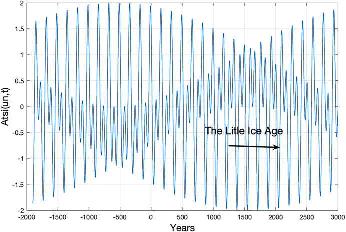
FIGURE 1. Constructive and destructive interference between Uranus-Neptune forced TSI index values, Atsi(un, t) = Atsi(ur, t) + Atsi(ne, t), for the years t = (−2000 … 3000). “The Little Ice Age” covers the six deepest Uranus-Neptune minima coincidences.

Saturn, Uranus, and Neptune (SUN) cycle periods (Tsa, Tur, Tun) have mean coincidences with the cycle periods: Tsun-mco = (169.84, 499.70, 999.39, 1960.96, 2450.84, 4289.61 4449.63) (yr.). From 1000 to 3000 A.D., the TSI index, Atsi(t) = (Atsi(sa, t) + Atsi(ur, t) + Atsi(ne, t)), experienced computed Eq. 8 deep minima: (Atsi(t) < −2.8 for Atsi(t) = ((−2.90, 1210), (−2.87, 1385), (−2.92, 1710), (−2.92, 1885), (−2.79, 2211)).

Deep Solar Minima Coincidences

Real solar data from 1000 A.D. (Usoskin 2005) onward yield the following classified deep solar minima: (Oort (1010–1070), Wolf (1270–1340), Spörer (1390–1550), Maunder (1640–1720), and Dalton (1790–1820)). The ACRIM TSI time series from 1000 A.D. has estimated deep minima at Oort (1013–1074), Wolf (1263–1326), Spörer (1510–1571), Maunder (1636–1706), Dalton (1773–1833), and Next (2002–2063) (Velasco et al., 2015). Solar variations are related to destructive and constructive interference between the SUN cycles.

Solar minima are correlated with a negative constructive interference when SUN cycles have amplitude minima Eq. 8. Oort (UN min, for t = 1020–1070), Wolf 1 (SUN min, for t = 1197–1294), Wolf 2 (SUN min, for t = 1350–1398), Spörer (UN min, for t = 1523–1571), Maunder (SUN min, for t = 1696–1744), Dalton (SU min, for t = 1791–1804), Modern (SUN min, for t = 1850–1899), Next (UN min, for t = 2024–2072), Next deep (SUN min, for t = 2197–2245). Wolf, Spörer and Maunder have the SUN cycle constructive negative interference, while Oort and Next have the UN cycle constructive negative interference. Dalton has SU cycle constructive negative interference. SUN cycles have positive constructive interference in the modern warm time period of 1981–2024.

Solar Forced Sea Temperature Oscillations

The accumulation of heat in oceans transforms the solar forced spectrum Stsi Eq. 1 into a solar-forced sea surface temperature (SST) spectrum Ssst Eq. 2. The solar-forced sea surface amplitude variations are computed using the following simplified sea surface temperature model:

$\text{Asst}\left(\text{jsun},\text{t}\right)={\text{Ksst}}^{\ast }\cos \left(2\pi \left(\text{t}‐{\text{t}}_{\text{sst}}\right)/\text{Tsst}\right),(9)$

where Asst (jsun, t) = (Asst (ju, t), Asst (sa, t), Asst (ur, t), and Asst (ne, t)) represent solar-forced sea surface temperature amplitude variations. Ksst = (Kju, Ksa, Kur, Kne) = (−1, −1, −1, −1). The cycle periods Tsst = Ttsi, where Ttsi = Tjsun. The cycle phase reference t_sst = t_tsi - Tjsun/4. The SST amplitude index Asst(t) = (Asst (ju, t) + Asst (sa, t) + Asst (ur, t) + Asst (ne, t)) covers an envelope period controlled by constructive and destructive interference between Tsst cycle periods.

The SST index, Asst(t), has a maximum in year 600 and a minimum in 2825 A.D. The new 4450-year SST envelope period has phase shifts in the years: Asst-en(t) = ((min, −1624.49), (-0, −512), (max, 600), (−0, 1712), (min, 2825)). From t = 1000 … 3000. the SST index Eq. 9, Asst(t) = (Asst (sa, t) + Asst (ur, t) + Asst (ne, t), experienced sea temperature deep minima: (Asst(t) = < −2.3, for Asst(t) = ((−2,48, 1069), (−2.39, 1244), (−2.73, 1375), (−2.73, 1570), (−2.70, 1745), (−2.37, 1896), (−2.88, 2070), (−2.88, 2246)), and SST index maxima at (Asst(t) > 2.4, for Asst(t) = ((2.86, 1024), (2.76, 1379), (2.75, 1525), (2.47, 1850), (2.53, 2025)). From t = 1850 … 2100, the SST index Eq. 9 experienced the following minima and maxima: Asst(t) = ((1.35, 1875), (−2.37, 1896), (−2.19, 1921), (−1.14, 1981), (2.53, 2025), (−2.88, 2070)).

The modern SST index maximum Asst(t) = (2.53, 2025) is a 500-year event after the maximum Asst(t) = (2.75, 1525) and a 1000-year event from the SST index maximum Asst(t) = (2.86, 1024). The SST index deep minimum at Asst(t) = (-2.88, 2070) is the deepest SST index minimum since 1375 B.C. The amplitude shift from a 500-year Asst(t) maximum to a 3000-year Asst(t) minimum in only 45 years is caused by SUN cycle period phase shifts from constructive positive interference to constructive negative interference.

Lunar Forced Sea Temperature Oscillations

Earth Nutation Oscillations

There is a chain of events from the Earth´s axis nutation oscillations to lunar forced sea surface temperature (LST) oscillations. The Earth’s axis nutation spectrum, Sln (Tln, θln (t-t_ln)), has a harmonic period spectrum Tln = (1, 2, 3, 4, … )18.61 (yr.). The dominant 18.61-year cycle reached a major standstill maximum at the year t_ln = 1932.3 and a minimum at the year t_ln = 1932.3 + 18.61/2 = 1941.6. A wavelet spectrum analysis of Earth´s position in the y-direction identified the harmonic Earth nutation cycle period spectrum Tln = (1/15, 1/3, 1, 4)18.61 = (1.24, 6.31, 18.61, 74.42) (yr.) from 1845 to 2000 A.D. The unstable 1.24-year cycle is known as the Chandler cycle. The dominant cycles Tln = (18.61, 74.44) (yr.) have estimated maxima in the years t_ln = (1943, 1979) and minima in the years (1933, 1942) (Yndestad 2004).

Lunar Nodal Tide Oscillations

The nutation spectrum, Sln (Tln, θln (t-t_ln)), introduces a global lunar nodal tide spectrum, Slnt (Tlnt, θlnt (t-t_lnt)), as a standing wave between the pole and Equator. The vertical component follows the Earth nutation amplitude variations. The horizontal component influences the tidal current, which has maximum and minimum amplitudes at approximately 30° from the equator. The horizontal tide current has a phase lag of approximately π/2 (rad). A wavelet spectrum analysis of the annual Aberdeen Sea level in North Atlantic water identified the lunar spectrum of Tlnt = (1/2, 1, 4)18.61 = (9.31, 18.61, 74.44) (yr.) in vertical amplitude variations. The estimated lunar nodal tide periods (18.61, 74.44) have minima in (1942, 1963) (Yndestad, 2006).

North Atlantic Water Oscillations

The stationary 18.61-year vertical and horizontal tide introduces a mix of warm surface sea temperatures with cold bottom temperatures; thus, heat is redistributed as a Tlnt = 18.6-year sea surface temperature cycle throughout the large-scale oceanic thermohaline system. A wavelet spectrum time-series analysis of the North Atlantic water temperature anomaly on the Scottish side of the Faroe-Shetland Channel from 1900 to 2005 revealed dominant periods of approximately (9, 18, 27, 36, 55, 75) years and indicated a strong harmonic cycle of approximately 9 years. The temperature cycle periods coincide with the lunar forced sea temperature period spectrum Tlst = (1/2, 2/2, 3/2, 4/2, 6/2, 8/2)18.61 years. The dominant periods (9, 18, 74) have maxima in (1940, 1942, 1943) (Yndestad, 2006).

Lunar Forced Sea Surface Amplitude Variations

Lunar forced sea surface temperature (LST) variations are represented as a transformation Eq. 3 of the Earth’s nodal spectrum, Tln, into a lunar forced sea surface temperature spectrum Slst (Alst(t), Tlst, Flst(t)). LST amplitude variations are computed using the following simplified sea surface temperature model:

$\text{Alst}\left(\text{t}\right)=\cos \left(2\pi \left(\text{t}-{\text{t}}_{\text{lst}}\right)/\text{Tlst}\right),(10)$

where the temperature variations are Alst(t) = (Alst (1, t), Alst (2, t), Alst (3, t)...). The cycle periods represent a harmonic spectrum: Tlst = (1/2, 2/2, 3/2, 4/2 … )18.61 = (9.31, 18.61, 27.92, 37.22, … ) (yr.). The lunar forced sea surface temperature cycle periods Tlst = (9.31, 18.61, 74.44) (yr.) has estimated maxima at the years t_lst = (1940, 1942, 1943) and minima in the years (1949, 1933, 1980). The 18.61-year cycle coincides with the Earth nutation in the y-direction, and the 74.44-year cycle period has a reversed-phase. (Yndestad, 2006).

Solar Lunar Cycle Coincidences

The solar-lunar-forced sea surface temperature spectrum, Sslt = Ssst + Slst, has amplitude variations, Aslt(t), controlled by cycle period coincidences and cycle phase coincidences. Sola forced cycle periods, Tsst, and lunar forced cycle period, Tln, have coincidences of ((Tsa, 3Tln/2), (Tur, 9Tln/2), (2Tsa, 6Tln/2), (Tne, 18Tln/2)) = ((29.44, 27.92), (58.88, 55.83), (84.02, 83.76), (164.79, 167.52)) (yr.).

Solar forced sea temperature amplitude variations, Asst(t), Eq. 9 has minima and maxima at Asst(t) = ((min, 1890), (max, 2025), (min, 2070). Lunar forced amplitude variations, Alst(t), Eq. 10 has minima and maxima at Alst(t) = ((min, 1905), (max, 2017), (min, 2079), (min, 2054). The solar-lunar-forced temperature variations have a negative constructive interference from Asst(t) = (min, 1890) to Alst(t) = (min, 1905), constructive positive interference from Alst(t) = (max, 2017) to Asst(t) = (max, 2025), and negative constructive interference from Asst(t) = (min, 2070) to Alst(t) = (min, 2079).

The solar forced spectrum, Tsst, and the lunar forced spectrum have different properties. The solar forced spectrum, Tsst, is a coincidence spectrum of JSUN cycle periods. The lunar forced spectrum Tlst is a harmonic spectrum from the 18.61-year lunar cycle. The phase relation between solar forced cycle periods and lunar cycle periods is a time-variant process, which is never repeated. This means that global temperature variations, controlled by constructive and destructive interference between solar-forced and lunar-forced sea temperature variations, are time-variant coincidences, which are never repeated. Solar forced temperature variations and lunar forced temperature variations must therefore be estimated as single events. The single events may still be deterministic because JSUN cycles and lunar nodal cycles have deterministic cycle periods and phase relations.

Earth Temperature Oscillations From 1850 A.D.

The Earth’s global mean temperature increased by approximately 1.0°C from 1850 to 2020. The temperature underwent a cold time period from 1850 to 1920, increased from 1920 to 1940, cooled from 1940 to 1978 and then increased again from 1978 to 2020 (Figure 2). Figure 2 illustrates the close relation between the Earth’s global mean temperature and the global sea surface temperature since 1850. The sea surface temperature exhibits a pattern similar to that of the global mean temperature. The global land surface temperature time series reveals a different trend, exhibiting a cycle with temperatures colder than the global temperature from 1850 to 1910 and a cycle with temperatures warmer than the global temperature from 1980 to 2015, indicating that heat accumulates in the sea. Wavelet analyses show correlations among global temperature, solar variation, lunar forcing, and a yet unidentified source. Thus, Earth’s temperature variability spectrum may have a solar-forced temperature spectrum, a lunar-forced temperature spectrum or a spectrum from an unknown source Sert(t).

FIGURE 2

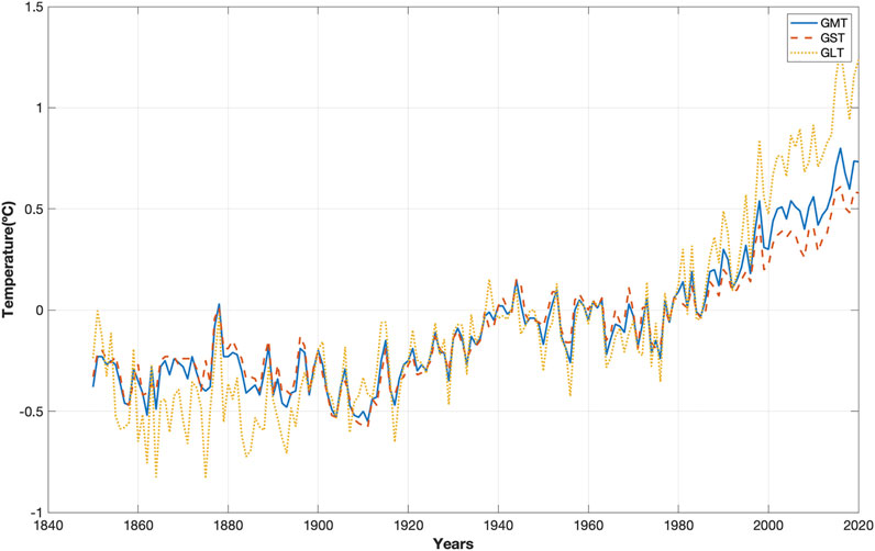
FIGURE 2. Earth’s global mean temperature, (GMT), (HadCRUT4), global sea surface mean temperature, (GST), (HadSST3) and global land surface mean temperature, (GLT), (CRUTEM4) from 1850 to 2020 (Climate Research Unit).

Global Sea Surface Temperature Oscillations

The global sea surface temperature (GST) (HadSST3) variability spectrum, Sgst (Tgst, θgst (t-t₀)), is transformed Eq. 5 into a wavelet spectrum Wgst (s, t). The wavelet spectrum, Wgst (s, t), is then computed for s = (1 … 85) and t = (1850 … 2020) (yr.), as shown in Figure 3. The computed GST wavelet spectrum, Wgst (s, t), has minima and maxima Wgst (s = min/max, t = (t₁,t₀)) = ((-2.2, 1860), (2.2, 1883), (-3.1, 1912), (3.0, 1943), (-3.9, 1977), (5.1, 2008)), at distances of (23, 29, 30, 34, 31) (yr.), and a mean cycle period of 58.8 years. The identified 58.8-year cycle in sea surface variability from 1850 coincides with the lunar forced cycles 3Tln = 55.83 years.

FIGURE 3

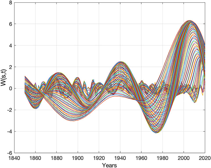
FIGURE 3. Global sea surface temperature (HadSST3) wavelet spectrum, Wgst (s, t), for s = (1 … 85) and t = (1850 … 2020) (yr.).

The stationary cycle periods in the wavelet spectrum Wgst (s, t) (Figure 4) are estimated by computing wavelet autocorrelations Eq. 7. The computed autocorrelations, WRgst (Rgst(s), m), of the wavelet spectrum, Wgst (s, t), have maximum correlations, Rgst = (0.20, 0.23, 0.20, 0.24, 0.30, 0.20, 0.12, 0.50, 0.23) with the stationary sea cycle surface periods Tgst = (9, 18, 28, 29, 37, 48, 57, 64, 74) (yr.) (Figure 5).

FIGURE 4

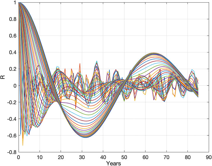
FIGURE 4. Global sea surface temperature wavelet autocorrelations: WRgst (Rgst(s), m) for s = (1 … 85) and m = (0 … 85) (yr.).

FIGURE 5

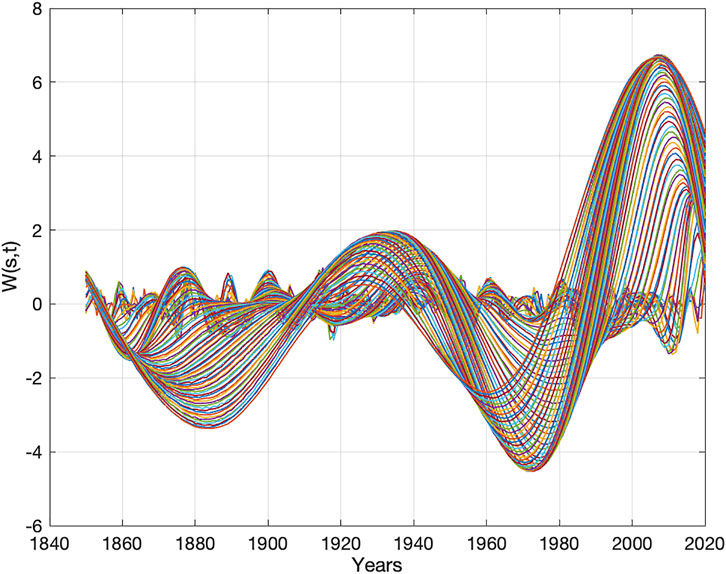
FIGURE 5. Global mean land temperature wavelet spectrum, Wglt (s, t), for s = (1 … 85) and t = (1850 … 2020) (yr.).

Solar Lunar Coincidences

The global sea surface temperature wavelet spectrum has a coincidence with the interference between deterministic solar forced cycle periods and lunar forced cycle periods. The estimated global sea surface temperature wavelet spectrum, Wgst (s, t), has coincidences with the deterministic lunar-forced sea surface spectrum, Slst, and the deterministic solar-forced sea surface temperature spectrum. Lunar-forced sea surface temperature spectrum Tlst = (9.3, 18.6, 27.9, 37.2, 46.5, 55.8, 65.1, 74.4) (yr.) has a coincidence with the identified stationary sea surface temperature periods Tgst = (9, 18, 28, 29, 37, 48, 57, 64, 74) (yr.), which confirms lunar-forced sea surface temperature variability. The identified 29-year cycle has a coincidence with the 29.44-year, Tsa, solar forced period.

The computed Eq. 5 global sea temperature wavelet spectrum, Wgst (s, t), has maximum and minimum at Wgst (s = max, min, t), = ((3.0, 1943), (-3.9, 1977)). The deterministic 74.44-year lunar forced temperature period has computed Eq. 10 maximum and minimum at Alst (74, t = (t₀, t₁)) = (1.0, 1942), (-1.0, 1979). The phase differences between the estimated sea surface temperature cycles and the deterministic lunar forced cycles are (1, 2) (yr.).

Lunar forced cycle periods Tlst = (18.61, 74.44) have minima at the years t = (1895, 1905, 1914) and a coincidence maximum at the year t = 2016. The solar forced SUN cycles have a minimum and maximum at Asst (t = (t₁, t₀)) = ((-2.37, 1896), (2.52, 2025)). The solar-forced minimum in 1896 has a coincidence with the lunar-forced minimum in 1895. The solar-forced SUN cycle has a maximum in 2025. The computed phase difference is one year. The lunar forced temperature cycles Tlst = (18.61, 74.44) have maxima in the time period 2007 to 2025 and coincidences with the solar forcing maximum in the year 2025.

Global Warming and Cooling

Global warming from 1895 to 2024 coincides with interference between solar-forced SST amplitude variations Eq. 9. The solar forced cycle SST index, Asst(t), has a minimum in 1895, the SST index, Asst(t), has a maximum in 2025, and coincides with sea temperature growth (Figure 2) and the wavelet spectrum, Wgst (s, t), amplitude minima and maxima (Figure 3). The solar forced cycles, Tsst, and lunar forced cycles, Tlst, show constructive negative interference in 1895 and positive constructive interference in 2025. The upcoming solar forcing SST index minimum is at Asst (t = t₁) = (−2.88, 2070), the deepest minimum since 1375 B.C., and has a destructive interference with the lunar forcing sea surface temperature at Alst (t = t₀) = (1.00, 2072).

Global Mean Temperature Oscillations

The Earth’s global mean temperature (GMT) time-series (HadCRUT4) variation is represented by the wavelet spectrum Wgmt (s, t). The wavelet spectrum, Wgmt (s, t), is computed for s = (1 … 85) and t = (1850 … 2020) (yr.). The computed wavelet spectrum, Wgmt (s, t), has the following minima and maxima: (Wgmt (s = min, max, t = (t₁, t₀)) = ((-2.0, 1860), (1.62, 1882), (-2.0, 1910), (2.4, 1941), (-4.0, 1974), (5.8, 2008)). These coincide with the global sea surface temperature, GST, and wavelet spectrum Wgst (s, t).

The autocorrelation spectrum, WRgmt (Rgmt(s), m), obtained from the wavelet spectrum, Wgmt (s, t), has maxima correlations, Rgmt (max) = (0.22, 0.23, 0.15, 0.27, 0.30, 0.20, 0.12, 0.38, 0.16), to the stationary global mean temperature cycle periods: Tgmt = (9, 18, 28, 29, 37, 46, 57, 64, 74) (yr.). The identified global mean temperature cycle spectrum, Tgmt, coincides with the identified global sea temperature cycles, Tgst, revealing that the global mean temperature variation is greatly influenced by the sea surface temperature variation.

Global Land Surface Temperature Oscillations

The global land surface temperature (GLT) (CRUTEM4) (Figure 2) variation is estimated from the wavelet spectrum Wglt (s, t). The wavelet spectrum, Wglt (s, t), is computed Eq. 5 for s = (1, … 85) and t = (1850, … 2020) (yr.). The computed GLT wavelet spectrum, Wglt (s, t), (Figure 5) has minima and maxima in (Wglt (s = (max, min)), Fglt) = ((−4.0, 1884), (2.0, 1934), (−4.5, 1972), (6.5, 2005)).

The computed autocorrelations Eq. 7, WRglt (Rglt(s), m), of the wavelet spectrum (Figure 6), Wglt (s, t), have maximum correlations, Rglt = (0.23, 0.18, 0.15, 0.20, 0.27, 0.13, 0.13, 0.23, 0.15, 0.28), to the identified stationary global land temperature cycle periods: Tglt = (9, 19, 28, 29.37, 47, 57, 64, 74, 81) (yr.).

FIGURE 6

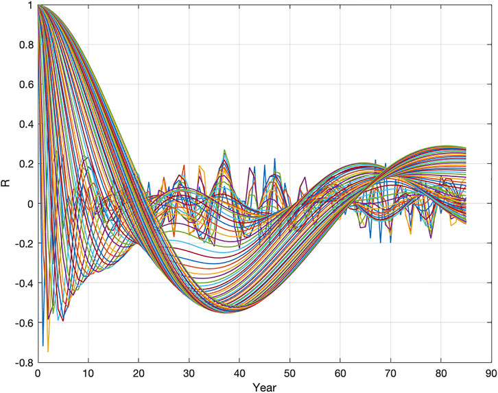
FIGURE 6. Autocorrelations of the global land temperature wavelet spectrum, WRglt (Rglt(s), m), for s = (1 … 85) and m = (1 … 85) (yr.).

Solar Lunar Coincidences

The identified stationary global land temperature spectrum, Tglt, coincides with the lunar forcing sea surface cycle periods, Tlst, and the solar forcing cycles (Tsa, Tur). Global land temperature variation and lunar-forced amplitude variations have reversed-phase coincidences. Lunar forced cycle periods have minima and maxima in the following years: Aglt (t = (t₀, t₁)) = ((−4.0, 1884), (1.0, 1885.8), (2.0, 1934), (−1.0, 1932.3)). Global land temperature cycles have minima and maxima in the following years: Alst (t = (t₁, t₀)) = ((−4.5, 1972), (1.0, 1978.8)), ((6.5, 2005), (−1.0, 2006.7)). The mean phase difference is only 2 years from 1884 to 2005.

After 1850, the TSI amplitude variation, Atsi(t), Eq. 8 has minima and maxima in Atsi(t = (t₁, t₀)) = ((−2.95, 1885), (2.36, 1930), (−1.00, 1974), (1.21, 2017), (−2.40, 2061)). The cycle-phase shift difference between global land temperature variations, Aglt(t), and the deterministic solar forcing amplitude variations, Atsi(t), Eq. 5 are as follows: Aglt (t = (t₁, t₀))—Atsi(t = (t₁, t₀)) = (1, 4, 2, 12) (yr.),with a mean phase difference of 2.3 years. The Saturn, Uranus (SU) cycles, (Tsa, Tur), show positive constructive interference in 2017 with a maximum of the GLT index, Aglt(t). Predictions of upcoming events show a deep minimum in 2061, when SUN forcing TSI cycles have negative constructive interference.

Greenland´S Temperature Oscillations From 2000 B.C.

The Greenland temperatures (GRT) are represented by the GISP2 time series (Figure 7), which covers the time period from 2000 B.C. to 1993 A.D. The mean Greenland temperature decreased from 1100 to 1750 A.D. and then began to increase. The temperatures also exhibit large fluctuations that appear to be random. These fluctuation properties are studied by transforming the time series into a wavelet power spectrum.

FIGURE 7

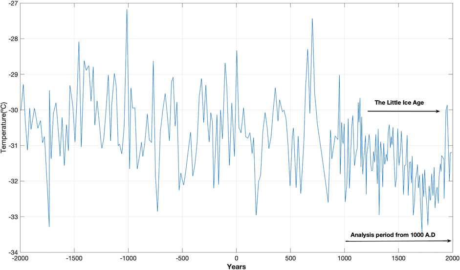
FIGURE 7. Greenland temperature (GISP2) time series spanning t = (−2000 … 1993) (yr.) and from t = (1000 … 1993) (yr.). “The Little Ice Age” is shown from approximately t = (1200 … 1850) (yr.).

Figure 8 depicts the Greenland temperature (GISP2) autocorrelation spectrum Eq. 7, WRgrt (Rgrt(s), m), of the wavelet spectrum Wgrt (s, t) for s = (1 … 500) and m = (1 … 500). The autocorrelation spectrum, WRgrt (Rgrt(s), m), starting in 1000 A.D., has maxima correlations, Rgrt = ((0.46, 0.43, 0.28, 0.21, 0.20, 0.26, 0.45), with stationary Greenland temperature cycle period: Tgrt = (18, 76, 147, 296, 334, 375, 446) (yr.).

FIGURE 8

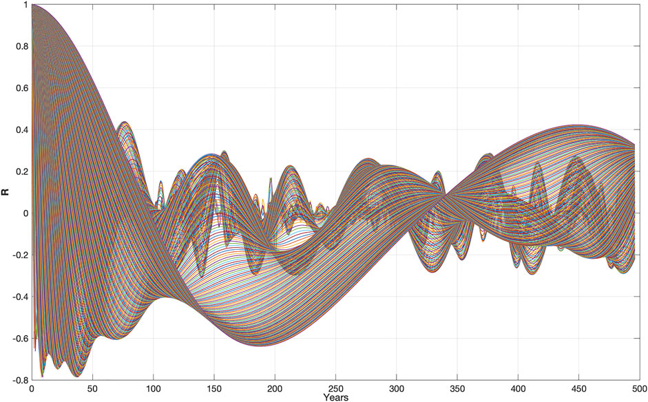
FIGURE 8. Greenland’s temperature (GISP2) wavelet autocorrelation spectrum, WRgrt (Rgrt(s), m), for s = (1 … 500) and m = (1...500) (yr.).

Solar Lunar Coincidences

Lunar-forced cycle periods have a spectrum: Tlst = (1, 4, 2*4, 4*4, 5*4, 6*4)Tln = (18.6, 74.4, 148.9, 297.8, 372.2, 446) (yr.). The coincident difference Terr = (Tgrt—Tlst) = (0, 1, 2, 3, 0) (yr.). The mean difference of one year confirms lunar-forced temperature variations have been occurring in Greenland for up to 446 years, controlled by the lunar nodal cycle period 4Tln = 74.44 years. The identified 334-year Greenland temperature cycle period has a coincidence with the solar-forced interference cycle Tun-mco (2) = 332.83 years.

Figure 9 shows the Greenland temperature (GISP2) wavelet power spectrum Eq. 6 for s = (1 … 500) and t = (1000 … 1993) (yr.). The wavelet power spectrum reveals the most dominant cycle in the wavelet spectrum, starting from 1000 A.D. The identified wavelet power spectrum has computed maxima of WPgrt (s = max, t = t₀) = ((71, 1129), (71, 1290), (93, 1502), (285, 1750), (124, 1979)), where the years 1290 and 1750 represent maxima in cold climate periods. A mean cycle period of 440 years confirms a stationary 446-year lunar forcing cycle in Greenland temperature variation. The computed wavelet power maximum, WPgrt (s = max, t = t₀) = (285, 1750) (Figure 9), reveals the deepest negative temperature event between 1000 and 2000 A.D. The 4450-year TSI envelope period, Atsi-en(t), has phase shifts in the years: Atsi-en(t) = ((−0, -1624.49), (max, −512), (+0, 600), (min, 1712), (−0, 2825)). The phase lag from the deterministic TSI envelope minimum in 1712 to the estimated Greenland temperature minimum in 1750 is 38 years.

FIGURE 9

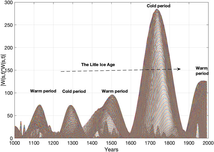
FIGURE 9. Greenland’s GISP2 temperature wavelet power spectrum, WPgrt (s, t), for s = (1...500) and t = (1000 … 1993) (yr.). The wavelet power spectrum shows dominant warm cycles and cold cycles from 1000 A.D., and the “The Little Ice Age” from approximately t = (1200 … 1850) (yr.).

Solar Lunar-Forced Interference From 1000 A.D.

The identified lunar-forced 446-year Greenland temperature cycle and the solar-forced SST cycle Eq. 9, Tun-mco (2) = 332.83, has a (3, 4) cycle coincidence interference in a total cycle of 1320 years. The 333-year solar-forced sea surface temperature cycle Eq. 9 and the 446-year lunar-forced sea surface temperature cycle experience computed positive constructive interference in (590–500) B.C., destructive interference in (1000–1160), negative constructive interference in (1330–1420) and (1660–1825), positive constructive interference in (1864–1995) and negative constructive interference in (2085–2160). The solar-forced sea temperature index, Asst(t), Eq. 9 has a minimum at Asst (t = t₁) = (−2.70, 1745), which coincides with the Greenland temperature minimum in 1750 (Figure 9) (Figure 11). The positive constructive interference time period 1864–1995 is known as a “modern warm time period”. The negative constructive interference occurring from (2085–2160) represents a computed upcoming cold time period.

Solar Lunar-Forced Interference From 2000 B.C.

From 2000 B.C., Greenland’s temperature wavelet power spectrum Eq. 6, WPgrt (s, t), for t = (-2000 … 1993) (yr.) and s = (1...2000) has maxima of WPgrt (s = max, t = t₀) = ((200, −1300), (120, −513), (147, 585), (392, 1620)), where the years 513 B.C. and 1620 A.D. represent maxima in cold climate periods. (Figure 10). The time period spanning from 513 B.C. to 1620 A.D. covers a total time period of 2133 years. The stationary temperature cycle, Tgrt (7), has computed phase shifts in the years: Agrt(t = (t₁, t₀)) = ((min, −513), (max, 554), (+0, 1086), (min, 1620), (−0, 2153), (max, 2686)).

FIGURE 10

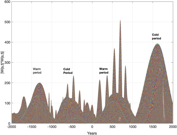
FIGURE 10. Greenland’s GISP2 temperature wavelet power spectrum, WPgrt (s, t), for t = (−2000 … 1993) (yr.) and s = (1...2000). The wavelet power spectrum shows dominant warm time periods and cold time periods from 2000 B.C.

The identified stationary 2133-year Greenland temperature cycle period from 2000 B.C. has a (2, 1) interference with the solar-forced envelope period Tun-mco (7) = 4285 years. The 2133-year Greenland temperature cycle and the 4285-year solar-forced cycle, Tun-mco (7), show destructive interference in 512 B.C. and negative constructive interference in 1620 A.D.

Solar Lunar-Forced Coincidences to “the Little Ice Age”

The Greenland temperature variation from 1000 A.D. (Figures7, 9) is controlled by the solar-forced UN sea surface temperature periods, (Tsst-mco (8), Tsst-mco (7)/2, Tsst-mco (2) = (4450, 2142, 333) (yr.), and the lunar forced sea temperature period, Tlst () = 446 years (Figure 11). The 332-year solar forced cycle and the 446-year lunar forced cycle have positive constructive interference in the years 165–320, destructive interference in 600–1160, and negative constructive interference in 1330–1420 and 1660–1825. The solar-lunar cycle periods have a computed upcoming negative constructive interference from 2085 to 2150 A.D. (Figure 11). Temporary negative constructive interference between the identified solar-lunar cycles indicates that “The Little Ice Age” covers a total time period of 820 years from 1330 to 2150 A.D.

FIGURE 11

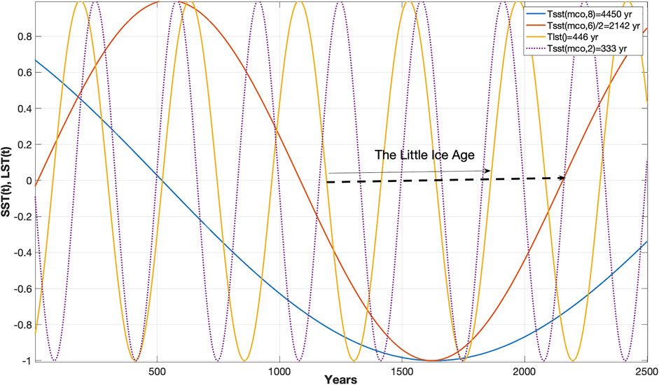
FIGURE 11. Stationary solar forced sea temperature cycler [Tsst (mco, 8], Tsst-mco (7)/2, Tsst-mco (2) = (4450, 2142, 333) (yr.) and lunar forced temperature period, Tlst, of 446 years in the time period t = (0 … 2500).

Discussion

Solar Forced Oscillations

The origin of total solar irradiation variation is not well understood. Mörth and Schlamminger (1979) investigated the relation between planetary motion, sunspots and climate and assumed that the transmission of gravitational torque in the solar system causes changes in the solar photosphere. This study of solar irradiation variation is based on a deterministic JSUN cycle spectrum model. The study reveals that TSI oscillation may be computed by the simple linear spectrum transform from JSUN cycle period oscillations to TSI cycle period oscillations. The TSI amplitude variations have minima when the JSUN cycles have perihelion coincidences and maxima when the JSUN cycles have aphelion coincidences. The total envelope time period covers a cycle period of 4450 years.

The computed TSI index Eq. 8 has minima coincidences to known deep solar minima from 1000 A.D. (Usoskin 2005), (Velasco et al., 2015). The new information from this study is deep solar minima coincidences with negative constructive interference between SUN cycles. Wolf, Spörer and Maunder have SUN cycle constructive interference, Oort has UN cycle constructive interference, and Dalton has SU cycle constructive interference. SUN cycles have negative constructive interference in the cold time period 1850–1899 and positive constructive interference in the modern warm time period 1981–2025. Solar deep minima amplitude variations are controlled by SUN perihelion coincidences in distances of Tsun-mco years. The Maunder minimum is a one-time event in the SUN envelope time period of 4450 years. The TSI envelope time period has a JSUN cycle minimum in 1712 A.D. coincident with the “Deep Freeze” year in 1709, when the winter temperature in Europe dropped to −15°C. (Sánchez Arreseigor, 2019).

Computed TSI variations coincide with solar activity (Kremliovsky 1994), (Bhowmik and Nandy 2018), (Velasco et al., 2021). Courtillot et al. (2021) identified Jovian cycles in solar activity and estimated an upcoming Solar Cycle 25 maximum in 2026. In upcoming events, SUN cycles have positive constructive interference in 1980–2000, and SU cycles have positive constructive interference in 2007–2025. The upcoming computed Eq. 8, the next solar minima have UN-type negative constructive interference from 2025 to 2072 and SUN-type negative constructive interference from 2197 to 2245. Stationary cycles in the ACRIM TSI time series from 1700 reveal a computed Next Dalton-type TSI minimum in 2035–2065 and a deep solar minimum in 2049 A.D. (Yndestad and Solheim 2017). Zharkova (2020) estimated an upcoming Maunder-type solar minimum time period from 2020 to 2053 A.D. (Velasco et al., 2022).

Solar-Forced Accumulation of Heat in Oceans

The study reveals a direct relation between the computed solar-forced sea temperature spectrum and the estimated global sea surface spectrum (Table 1 and Table 2). The direct relation confirms the linear spectrum transform Eq. 2, where the solar forced cycle periods coincide with the TSI cycles and Jovian planet cycles. A π/2 (rad) phase lag in the accumulation of heat from solar-forced TSI cycles introduces a new constructive and destructive interference between solar-forced sea surface temperature cycles.

TABLE 1

TABLE 1. Cycle- and phase-coincidences between Jovian planet oscillations (JSUN), total solar irradiation oscillations (TSI) and lunar nodal forced sea temperature oscillations (LST).

TABLE 2

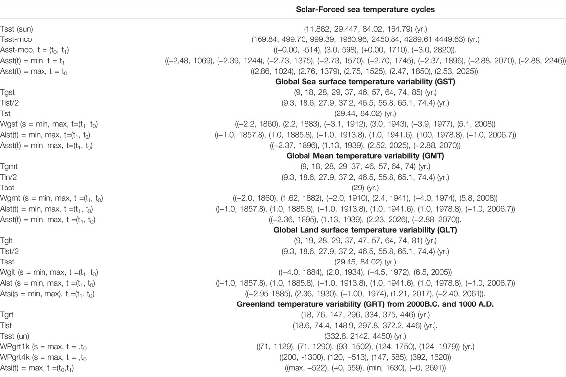
TABLE 2. Cycle- and phase-coincidences between stationary solar-forced sea temperature cycles (GST), global sea surface temperature cycles (GST), global mean temperature cycles (GMT), global land temperature cycles (GLT) and Greenland temperature cycles (GRT).

New phase relations between Jovian planet cycles have unexpected influences on climate variations. The modern warm cycle in 1920–2050 coincides with positive UN cycles Eq. 9. SUN cycles have positive constructive interference in 2025. The computed SST index (2.53, 2025) has the highest sea surface temperature index in 500 years, which reveals that the modern warm time period is a rare event controlled by the solar forced accumulation of heat in oceans. The 45-year SST index shift, from a 500-year maximum in 2025 to a 3000-year index minimum in 2070, is caused by a rare phase shift relation between the SUN cycles. The computed solar-forced deep minimum in 2070 indicates an upcoming deep cold climate period.

A wavelet spectrum analysis of the Arctic ice edge position from 1579 to 2020 revealed a computed upcoming maximum ice extent in 2073 (Yndestad 2021). A.D. Yu et al. (2011) published a study of variations in Earth temperatures over the past 2485 years. The study was based on a power spectrum analysis of temperature variations based on tree rings and predicted that temperatures will decrease in the future until 2068 A.D. and then increase again.

Lunar Forced Oscillations

The lunar-forced temperature variability is explained by a lunar-forced tidal vertical mixing process in oceans and interference between lunar-forced temperature cycles in the thermohaline circulation flow. Maksimov and Smirnov (1967) estimated a global standing 19-year tide in the Atlantic Ocean. The identified standing lunar node tide had a maximum amplitude at the Arctic pole, a 50% maximum amplitude at the equator and a zero-amplitude node at 35 degrees latitude. This study has revealed cycle period- and cycle phase coincidences between the Earth axis nutation spectrum in the y-direction, the lunar nodal tide, North Atlantic water temperature variations, Earth’s global temperature variations from 1850 and Greenland temperature variations from 2000 B.C. This close relation confirms the simplified lunar forced sea surface spectrum model. Greenland temperature variation reveals lunar-forced temperature cycles of up to 446 years and controlled subharmonic periods from the 74.44-year lunar cycle. The 74.44-year cycle is confirmed in the NAO index and Arctic data series (Yndestad 2006).

Global Temperature Oscillations

Global sea surface variability is controlled by the interreference between the solar-forced spectrum and the lunar-forced spectrum. The wavelet spectrum analysis of global temperature variations from 1850 confirms the hypothesis from Eq. 4 (Table 2). The global temperature variations from 1850 to 2020 have coincides with constructive and destructive interference between solar forced cycle periods and lunar forced cycle periods. Solar lunar forced coincidence to Greenland temperature variations from 2000 B.C. indicate that global sea surface temperature is period- and phase-locked to the 4450-year solar forced envelope period. The implication of interference is temporary warm and cold climate periods. The solar-forced sea temperature index computes a 500-year modern temperature maximum in 2025 and an upcoming 3000-year deep minimum temperature in 2070. The implication of this deep minimum is unclear.

Global Mean Temperature Variability

Global mean temperature variation coincides with the global sea temperature variation spectrum, revealing a major influence from the latter. Solar-lunar-forced interference in the oceans explains the origin of Earth’s climate variation, with multidecadal cycles as a major cause of the global temperature variations that occurred from 1850 to 2020. The global sea surface temperature has approximately the same variation in the Northern and Southern Hemispheres. This confirms lunar forced cycles as a global standing wave and a coherent source of heat distribution in the oceans and solar forced TSI cycles as a coherent source of accumulated heat in the oceans (Table 2). Solar-forced temperature cycles and lunar-forced temperature cycles have different properties in the global temperature grid. Coherent solar forced cycles accumulate, while lunar forced cycles have phase variations in the global grid. This difference explains why lunar forced cycles have correlation R-values of 0.2–0.5 to the global temperature time series.

In this study, global sea surface temperature has an estimated amplitude maximum in 1941. Kravstov et al. (2018) suggested that the North Atlantic Ocean is the major center of the Global Multidecadal Oscillation. The Atlantic Multidecadal Oscillation index has a maximum in 1942. The North Atlantic Water (NAW) inflows to the Norwegian Sea and has a maximum in 1943 (Yndestad et al., 2008).

Global Land Temperature Variability

The identified global land surface temperature spectrum has a TSI forced spectrum and a lunar forced spectrum. A direct relation to the TSI spectrum explains why the global land surface temperature time series reveals a different trend, exhibiting a time period with temperatures colder than the global temperature from 1850 to 1910 and a warmer period from 2000 to 2020 (Figure 2). The lunar-forced spectrum in the global land surface spectrum may be explained by the wind-driven heat from global sea surface temperature variation. The lunar-forced land surface temperature variations and lunar force sea surface temperature variations have reversed-phase relations. A possible explanation is a π/2 (rad) phase lag from sea surface temperature to air temperature and a new π/2 (rad) phase lag in the integration of heat into land surface temperature.

Greenland Temperature Oscillations

Greenland’s temperature variation is controlled by the NAW temperature and the North Atlantic Oscillation (NAO) (Vinther 2006; Vinther et al., 2003, 2010). The NAO winter index variation has a lunar-forced cycle spectrum that coincides with the North Atlantic Water inflows to the Norwegian Sea, the Barents Sea and the Arctic Sea ice extent (Yndestad 2006). These close relations among the global temperature variation, North Atlantic water temperature and Greenland temperature confirm the close relation between Greenland’s temperature variation and the global sea surface temperature variation.

Greenland temperature variation coincides with solar- and lunar-forced sea temperature variability. Lunar forced temperature periods are subharmonic periods from the 74.44-year lunar period up to 446 years. Long cycle periods in Greenland temperature variations (Figure 9, Figure 10) have cycle periods and cycle phase coincidences to solar-forced sea surface periods of 333, 2142 and 4450 years (Figure 11). Negative constructive interference between the solar-lunar-forced sea temperature period explains temporary cold and warm climate periods from 1330 to 2150 A.D. (Figure 11). The next upcoming cold period has negative constructive interference from 2085 to 2150 A.D. Longer cycle periods continue the computed solar forced minimum in 2072. A wavelet spectrum analysis of Arctic ice extent from 1579 confirms a 223-year lunar forced cycle and a computed upcoming maximum ice extent in 2073 A.D. (Yndestad 2021).

Ljungqvist (2010) reconstructed temperature variability in the Northern Hemisphere (30–90°N) based on 30 proxy records during the last two millennia and identified a warm time period in the years 1–300, a cold time period 300–800, a warm time period 800–1300 and a cold time period in the years 1300–1900. The Briksdal glacier in the western part of Norway began to grow in 500 B.C. and reached its maximum extent in 1755 A.D. (Burki et al., 2009). The Greenland temperature power spectrum has a deep minimum in 1750 A.D. (Figure 9).

Conclusions

This study suggests that Earth’s global temperature variabilities starting in 1850 and Greenland temperature variabilities starting in 2000 B.C. have solar-lunar-forced stationary temperature cycles up to 4450 years. The primary causes of the identified multidecadal temperature variation is the stationary orbital cycles from the Jovian planets (Jupiter, Saturn, Uranus, Neptune) and the 18.6-year lunar nodal cycle from the Earth’s axis nutation.

Solar Lunar Spectrum Transformations

The chain of events from Jovian planet oscillations and the Earth’s axis nutation oscillations may be represented as linear spectrum transformations of cycle periods and cycle period phase relations. The Jovian planet oscillation spectrum may be transformed into a solar irradiation spectrum and a solar forced sea surface temperature spectrum. The Earth’s nutation oscillation spectrum may be transformed into a lunar forced sea surface temperature spectrum.

Solar Lunar Cycle Interference

This study has revealed the importance of cycle period phase relations in climate variations. TSI amplitude variations coincide with constructive and destructive interference between Jovian planet cycles in an envelope period of 4450 years. The TSI envelope period has a minimum when JSUN periods have perihelion coincidences and a maximum when JSUN periods have aphelion coincidences. The accumulation of solar-forced heat in oceans introduces a π/2 (rad) phase lag in solar-forced sea temperature cycles and a new envelope cycle of solar-forced minima and maxima temperatures. Temperature variations from 2000 B.C. coincide with constructive and destructive interference between solar-forced and lunar-forced temperature variations. Solar lunar-forced global temperature cycles have time-variant phase relations and time-variant interference. The time-variant climate variations are never repeated. Climate variation may still be deterministic because the Jovian planet cycles and the Earth nutation cycles have approximately deterministic period and phase relations.

Sola Lunar-Forced Global Earth Temperature Variations Since 1850

Global temperature variations from 1850 to 2020 (Climate Research Unit) coincide with interference between solar lunar forced cycles. The global sea surface temperature (HadSST3) variability spectrum coincides with interference between solar-forced and lunar-forced sea temperature variations. The sea temperature variations from 1890 to 2020 coincide with a solar forced sea temperature minimum in 1896 and a solar forced sea temperature maximum in 2025. In terms of upcoming events, computations suggest the sea surface temperature will have a deep minimum in 2070.

Sea surface temperature and global mean temperature (HadCRUTE4) have cycle period coincidences and cycle phase coincidences. The spectrum coincidence confirms that sea surface temperature has a major influence on global temperature variations. Global land temperature (CRUTEM4) variation coincides with interference between solar forced irradiation cycles and lunar forced temperature cycles. The solar forced irradiation spectrum has a direct influence on Earth’s global land surface temperature variations. The lunar forced temperature variations are explained by wind-driven heat from sea surface temperature variations.

Solar Lunar Forced Temperature Variations in Greenland From 2000 B.C.

Greenland’s temperature (GISP2) variations and North Atlantic temperature variations are closely related to global sea surface temperature variations. The variation in Greenland’s temperature, beginning in 2000 B.C., reflects solar-lunar-forced interference cycles up to 4450 years. The Greenland temperature variation has lunar forced cycle periods up to 446 years, solar forced sea temperature cycles of 333 and 2142 years and a 4450-year TSI envelope cycle. The 4450-year envelope cycle has a minimum in 1745 when the identified Greenland temperature variation is at a minimum. Negative constructive interference between the identified solar-lunar cycles indicates that “The Little Ice Age” covers temporary cold periods from 1330 to 2150 A.D. The next upcoming negative constructive interference period covers the computed time period from 2070 to 2150.

Data Availability Statement

Publicly available datasets were analyzed in this study. This data can be found here: and; Climatic Research Unit (http://www.metoffice.gov.uk/hadobs/hadcrut4/). Paleoclimatology Program (https://www.ncdc.noaa.gov/data-access/paleoclimatology-data) (Kobashi et al. 2011).

Author Contributions

The author confirms being the sole contributor of this work and has approved it for publication.

Conflict of Interest

The authors declare that the research was conducted in the absence of any commercial or financial relationships that could be construed as a potential conflict of interest.

Publisher’s Note

All claims expressed in this article are solely those of the authors and do not necessarily represent those of their affiliated organizations, or those of the publisher, the editors and the reviewers. Any product that may be evaluated in this article, or claim that may be made by its manufacturer, is not guaranteed or endorsed by the publisher.

References

Abreu, J. A., Beer, J., Ferriz-Mas, A., McCracken, K. G., and Steinhilber, F. (2012). Is There a Planetary Influence on Solar Activity? Astron. a Astrophysics 548, A88. doi:10.1051/0004-6361/201219997

CrossRef Full Text | Google Scholar

Bhowmik, P., and Nandy, D. (2018). Prediction of the Strength and Timing of sunspot Cycle 25 Reveal Decadal-Scale Space Environmental Conditions. Nat. Commun. 9 (5209), 5209–5210. doi:10.1038/s41467-018-07690-0

PubMed Abstract | CrossRef Full Text | Google Scholar

Burki, V., Eiliv, L., Ola, F., and Nesje, A. (2009). Glacial Remobilization Cycles as Revealed by Lateral Moraine Sediment, Bødalsbreen Glacier Foreland, Western Norway. The Holocene 19 (3), 415–426.

CrossRef Full Text | Google Scholar

Charvátová, I. (2000). Can Origin of the 2400-year Cycle of Solar Activity Be Caused by Solar Inertial Motion? Ann. Geophysicae 18, 399–405.

Google Scholar

Courtillot, V., Lopes, F., and Le Mouël, J. L. (2021). On the Prediction of Solar Cycles. Sol. Phys. 296, 21. doi:10.1007/s11207-020-01760-7

CrossRef Full Text | Google Scholar

Currie, R. G. (1981). Evidence for 18.6 Year (Sic) Signal in Temperature and Drought Conditions in North America since A. D. 1800. J. Geophys. Res. 86 (11), 055. doi:10.1029/jc086ic11p11055

CrossRef Full Text | Google Scholar

Daubechies, I. (1992). Ten Lectures of Wavelet. SIAM J. Math. Anal. 24, 499–519.

Google Scholar

Egbert, G. D., and Ray, R. D. (2000). Significant Dissipation of Tidal Energy in the Deep Ocean Inferred from Satellite Altimeter Data. Nature 405, 775–778. doi:10.1038/35015531

PubMed Abstract | CrossRef Full Text | Google Scholar

Fairbridge, R. W., Sanders, J. E., et al. (1987). “The Sun’s Orbit, AD 250–2050: Basis for New Perspectives on Planetary Dynamics and Earth-Moon Linkage.” in Bibliography 475–541, editor M. R. Rampino, 446–471.

Google Scholar

Gratiot, N., Anthony, E. J., Gardel, A., Gaucherel, C., Proisy, C., and Wells, J. T. (2008). Significant Contribution of the 18.6 Year Tidal Cycle to Regional Coastal Changes. Nat. Geosci 1 (3), 169–172. doi:10.1038/ngeo127

CrossRef Full Text | Google Scholar

Gustavo, R., Ernesto, J., Esther, N., and Soon, W. W. (2018). Lunar Fingerprints in the Modulated Incoming Solar Radiation: In Situ Insolation and Latitudinal Insolation Gradients as Two Important Interpretative Metrics for Paleoclimatic Data Records and Theoretical Climate Modeling. New Astron. 58, 96–106. doi:10.1016/j.newast.2017.08.003

CrossRef Full Text | Google Scholar

Hansen, J. M., Aagaard, T., and Kuijpers, A. (2015). Sea-Level Forcing by Synchronization of 56- and 74-Year Oscillations with the Moon's Nodal Tide on the Northwest European Shelf (Eastern North Sea to Central Baltic Sea). J. Coastal Res. 315, 1041–1056. doi:10.2112/JCOASTRES-D-14-00204.1

CrossRef Full Text | Google Scholar

Hoyt, D. V., and Schatten, K. H. (1993). A Discussion of Plausible Solar Irradiance Variations, 1700-1992. J. Geophys. Res. 98, 18895–18906. doi:10.1029/93ja01944

CrossRef Full Text | Google Scholar

Jose, P. D. (1965). Sun's Motion and Sunspots. Astron. J. 70, 193–200. doi:10.1086/109714

CrossRef Full Text | Google Scholar

Keeling, C. D., and Whorf, T. P. (1997). Possible Forcing of Global Temperature by the Oceanic Tides. Proc. Natl. Acad. Sci. U.S.A. 94, 8321–8328. doi:10.1073/pnas.94.16.8321

PubMed Abstract | CrossRef Full Text | Google Scholar

Kobashi, T., Kawamura, K., Severinghaus, J. P., Barnola, J.-M., Nakaegawa, T., Vinther, B. M., et al. (2011). High Variability of Greenland Surface Temperature over the Past 4000 Years Estimated from Trapped Air in an Ice Core. Geophys. Res. Lett. 38 (21), a–n. doi:10.1029/2011GL049444

CrossRef Full Text | Google Scholar

Kravtsov, S., Grimm, C., and Gu, S. (2018). Global-scale Multidecadal Variability Missing in State-Of-The-Art Climate Models. Npj Clim. Atmos. Sci. 1, 34. doi:10.1038/s41612-018-0044-6

CrossRef Full Text | Google Scholar

Kremliovsky, M. N. (1994). Can We Understand Time Scales of Solar Activity? Sol. Phys. 151, 351–370. doi:10.1007/bf00679081

CrossRef Full Text | Google Scholar

Liu, Y., Cai, Q. F., Song, H. M., An, Z. S., and Linderholm, H. W. (2011). Amplitudes, Rates, Periodicities and Causes of Temperature Variations in the Past 2485 Years and Future Trends over the central-eastern Tibetan Plateau. Chin. Sci. Bull. 56, 28–29. doi:10.1007/s11434-011-4713-7

CrossRef Full Text | Google Scholar

Ljungqvist, F. C. (2010). A New Reconstruction of Temperature Variability in the Extra‐tropical Northern Hemisphere during the Last Two Millennia. Geogra!ska Annaler: Ser. A, Phys. Geogr. 92 (3), 339–351. doi:10.1111/j.1468-0459.2010.00399.x

CrossRef Full Text | Google Scholar

Maksimov, I. V., and Smirnov, N. P. (1967). A Long-Term Circumpolar Tide and its Significance for the Circulation of Ocean and Atmosphere. Oceanology 7, 173–178. (English edition).

Google Scholar

Maksimov, I. V., and Smirnov, N. P. (1964). Long-range Forecasting of Secular Changes of the General Ice Formation of the Barents Sea by the Harmonic Component Method. Murmansk Polar Sci. Res. Inst. Sea Fish. 4, 75–87.

Google Scholar

Mann, M. E., Steinman, B. A., and Miller, S. K. (2020). Absence of Internal Multidecadal and Interdecadal Oscillations in Climate Model Simulations. Nat. Commun. 11, 49. doi:10.1038/s41467-019-13823-w

PubMed Abstract | CrossRef Full Text | Google Scholar

MATLAB (2020). MATLAB. Wavelet Toolbox. Users Guide. Portola Valley, CA, USA: The Math Works Inc.

Google Scholar

McCracken, K. G., Beer, J., and Steinhilber, F. (2014). Evidence for Planetary Forcing of the Cosmic Ray Intensity and Solar Activity throughout the Past 9400 Years. Sol. Phys. 289 (8), 3207–3229. doi:10.1007/s11207-014-0510-1

CrossRef Full Text | Google Scholar

Morice, C. P., Kennedy, J. J., Rayner, N. A., and Jones, P. D. (2012). Quantifying Uncertainties in Global and Regional Temperature Change Using an Ensemble of Observational Estimates: The HadCRUT4 Data Set. J. Geophys. Res. 117, a–n. doi:10.1029/2011JD017187

CrossRef Full Text | Google Scholar

Mörth, H. T., and Schlamminger, L. (1979). Planetary Motion, Sunspots and Climate, Solar-Terrestrial Influences on Weather and Climate. Dordrecht: Springer.

Google Scholar

Pettersson, O. (1914). Climatic Variations in Historic (Sic) and Prehistoric Time: Svenska Hydrogr. Biol. Kommissiones Skrifter 5, 26.

Google Scholar

Pettersson, O. (1915). Long Periodical (Sic) Variations of the Tide- Generating Force. Publ. Circular Conseil Permanent Int. pour l’Exploration de la Mer 65, 2e23.

Google Scholar

Pettersson, O. (1905). On the Probable Occurrence in the Atlantic Current of Variations Periodical, and Otherwise, and Their Bearing on Metrological and Biological Phenomena. Rapports Proce’s- Verbaux des Re’unions de Conseil Permanent Int. pour l’Exploration de la Mer 42, 221e240.

Google Scholar

Sánchez Arreseigor, J. S. (2019). Winter Is Coming: Europe's Deep Freeze of 1709 Published on July 8, 2019 National Geographic.

Google Scholar

Satterley, A. (1996). The Interpretation of Cyclic Successions of the Middle and Upper Triassic of the Northern and Southern Alps. Earth-Science Rev. 40, 181–207. doi:10.1016/0012-8252(95)00063-1

CrossRef Full Text | Google Scholar

Scafetta, N. (2016). High Resolution Coherence Analysis between Planetary and Climate Oscillations. Adv. Space Res. 57 (10), 2121–2135. doi:10.1016/j.asr.2016.02.029

CrossRef Full Text | Google Scholar

Scafetta, N., Milani, F., Bianchini, A., and Ortolani, S. (2016). On the Astronomical Origin of the Hallstatt Oscillation Found in Radiocarbon and Climate Records throughout the Holocene. Earth-Science Rev. 162, 24–43. doi:10.1016/j.earscirev.2016.09.004

CrossRef Full Text | Google Scholar

Scafetta, N. (2012). Multi-scale Harmonic Model for Solar and Climate Cyclical Variation throughout the Holocene Based on Jupiter-Saturn Tidal Frequencies Plus the 11-year Solar Dynamo Cycle. J. Atmos. Solar-Terrestrial Phys. 80, 296–311. doi:10.1016/j.jastp.2012.02.016

CrossRef Full Text | Google Scholar

Steinhilber, F., and Beer, J. (2013). Prediction of Solar Activity for the Next 500 Years. J. Geophys. Res. Space Phys. 118, 1861–1867. doi:10.1002/jgra.50210

CrossRef Full Text | Google Scholar

Suess, H. E. (1980). The Radiocarbon Record in Tree Rings of the Last 8000 Years. Radiocarbon 22, 200–209. doi:10.1017/s0033822200009462

CrossRef Full Text | Google Scholar

Torrence, C., and Compo, G. P. (1998). A Ptactical Guide to Wavele Analysis. Boulder, CO 80307-3000: National Center for Atmospheric Research, P.O. Box 3000.

Google Scholar

Usoskin, I. G. (2005). A History of Solar Activity over Millennia. Living Rev. Solar Phys. 5 (1), 1–88. doi:10.12942/lrsp-2013-1

CrossRef Full Text | Google Scholar

Velasco Herrera, V. M., Mendoza, B., and Velasco Herrera, G. (2015). Reconstruction and Prediction of the Total Solar Irradiance: from the Medieval Warm Period to the 21st century. New Astron. 34, 221–233. doi:10.1016/j.newast.2014.07.009

CrossRef Full Text | Google Scholar

Velasco Herrera, V. M., Soon, W., Hoyt, D. V., and Muraközy, J. (2022). Group Sunspot Numbers: A New Reconstruction of Sunspot Activity Variations from Historical Sunspot Records Using Algorithms from Machine Learning. Sol. Phys. 297, 8. doi:10.1007/s11207-021-01926-x

CrossRef Full Text | Google Scholar

Velasco Herrera, V. M., Soon, W., and Legates, D. R. (2021). Does Machine Learning Reconstruct Missing Sunspots and Forecast a New Solar Minimum? Adv. Space Res. 68, 1485.

Google Scholar

Vinther, B. M. (2006). Greenland and North Atlantic Climatic Conditions - as Seen in High Resolution Stable Isotope Data, (August).

Google Scholar

Vinther, B. M., Johnsen, S. J., Andersen, K. K., Clausen, H. B., and Hansen, A. W. (2003). NAO Signal Recorded in the Stable Isotopes of Greenland Ice Cores. Geophys. Res. Lett. 30 (7), 1–4. doi:10.1029/2002GL016193

CrossRef Full Text | Google Scholar

Vinther, B. M., Jones, P. D., Briffa, K. R., Clausen, H. B., Andersen, K. K., Dahl-Jensen, D., et al. (2010). Climatic Signals in Multiple Highly Resolved Stable Isotope Records from Greenland. Quat. Sci. Rev. 29 (3–4), 522–538. doi:10.1016/j.quascirev.2009.11.002

CrossRef Full Text | Google Scholar

Yndestad, H. (2021). Barents Sea Ice Edge Position Variability 1579-2020. Ålesund, Norway: NTNU-Ålesund. Mai 2010. doi:10.13140/RG.2.2.16122.41928

CrossRef Full Text | Google Scholar

Yndestad, H., and Solheim, J.-E. (2017). The Influence of Solar System Oscillation on the Variability of the Total Solar Irradiance. New Astron. 51, 135–152. doi:10.1016/j.newast.2016.08.020

CrossRef Full Text | Google Scholar

Yndestad, H. (2006). The Influence of the Lunar Nodal Cycle on Arctic Climate. ICES J. Mar. Sci. 63 (3), 401–420. doi:10.1016/j.icesjms.2005.07.015

CrossRef Full Text | Google Scholar

Yndestad, H., Turrell, W. R., and Ozhigin, V. (2008). Lunar Nodal Tide Effects on Variability of Sea Level, Temperature, and Salinity in the Faroe-Shetland Channel and the Barents Sea. Deep Sea Res. Oceanographic Res. Pap. 55 (10), 1201–1217. doi:10.1016/j.dsr.2008.06.003

CrossRef Full Text | Google Scholar

Zharkova, V. (2020). Modern Grand Solar Minimum Will lead to Terrestrial Cooling. Temperature (Austin) 7 (3), 217–222. doi:10.1080/23328940.2020.1796243

PubMed Abstract | CrossRef Full Text | Google Scholar

Zhenqiu, R., and Zhisen, L. (1980). Effect of Motions of Planets of Climate Changes in China Kexue Tongbao. Vol. 25 No. 5 May 1980. Beijing.

Google Scholar

Nomenclature

JSUN jupiter, Saturn, Uranus, Neptune

SUN saturn, Uranus, Neptune

UN uranus, Neptune

SU saturn, Uranus

SPO solar position oscillations

TSI total solar irradiation

SST solar forced sea temperature

LST lunar forced sea surface temperature

NAO north Atlantic Oscillation

Cycle is a series of events that lead back to the starting point y(t) = y(t + T)

Cycle period is the time taken to complete one cycle of an oscillation T = [t₀ … t_n]

Oscillation is a periodic variation for y(t) = y(t + kT) for k = 0, 1, 2, 3,…

Frequency is the number of occurrences of a repeating event per unit time f = 1/T

Angular frequency is the rate of change of angular displacement, θ (theta), or the rate of the change of the argument of the sine function or a cosine function y(t) = cos(θ(t)) = cos(ωt) = cos(2πft) = cos(2πt/T)

Cycle phase reference is the time when the cycle period has a maximum y(t) = cos(θ(t)-θ(t₀) = cos(ωt-ωt₀) = cos(2πft-2πft₀) = cos(2πt/T-2πt₀/T) = cos(2π(t-t₀)/T)

Cycle maximum and minimum reference y(t = (t₀, t₁))

Cycle phase shifts y(t) = (max, +0, min, -0), for t = (t₀, t₀+T/4, t₀+T/2, t₀+3T/4)

Interference two cycle periods [T₁, T₂] have constructive interference, y₁(t)+y₂(t) = max, when the cycle periods have phase coincidences θ₁(t₀) = θ₂(t₀) and destructive interference, y₁(t)+y₂(t) = 0, when the periods have reversed-phase coincidences θ₁(t₀) =-θ₂(t₀)

Cycle envelope period, of two cycle periods [T₁, T₂], is a smooth curve outlining its extremes y(t) = y₁(t)+y₂(t)

Spectrum is a classification on a scale between two extreme points

Cycle spectrum S(T, (θ(t-t₀)), where T = (T₁ … T_n), and θ(t-t₀) = (θ(t-t₀)₁ … θ(t-t₀)_n)

Cycle period k in a spectrum T(k) = (T₁ … T_k … T_n)

Harmonic cycle spectrum T_har = (T, 2T, 3 T … )

Cycle coincidence spectrum T_co = (A∗T₁ = B∗T₂ = C∗T₁)

Sjsun(Tjsun, θjsub(t-t₀)) jovian planets (Jupiter, Saturn, Uranus, Neptune) cycle spectrum

Ssst(Tsst, θsst(t-t₀)) solar forced Sea surface (SST) cycle spectrum

Sln(Tln, θln(t-t₀)) lunar Nodal (LN) cycle spectrum

Slst(Tlst, θlst(t-t₀)) lunar forced Sea surface (LST) cycle spectrum

Sglt(Tglt, θglt(t-t₀)) global Land surface temperature (GLT) cycle spectrum

Sgst(Tgst, θgst(t-t₀)) global Sea surface temperature (GST) cycle spectrum

Sgmt(Tgmt, θgmt(t-t₀)) global Mean Temperature (GMT) cycle spectrum

Sgrt(Tgrt, θgrt(t-t₀)) Greenland Temperature (GRT) cycle spectrum

Serr(Terr, θerr(t-t₀)) temperature cycle spectrum from an unknown source

Spectrum transfer function H(T_h, θ_h(t_h)) = H(T₂/T₁, θ_h(t_h))= θ₁(t₁)-θ₂(t₂))

Spectrum transformation S₂(T₂, = T_h∗T₁, θ₂(t₁-t_h)) = H(T_h, θ₁(t_h))S₁(T₁, θ₁(t₁))

Hsun(Tsun, θsun(t_sun)) linear transform of JSUN cycles to TSI cycles

Hoce(Toce, θoce(t_oce)) linear transform of Earth nutation cycles to LSR cycles

Wglt(s, t)) global land surface temperature wavelet spectrum

Wgst(s, t)) global sea surface temperature wavelet spectrum

Wgms(s, t)) global mean surface temperature wavelet spectrum

Wgrt(s, t)) greenland temperature wavelet spectrum

WPgrt(s, t)) greenland temperature wavelet power spectrum

WAglt(R, m)) global land surface temperature wavelet autocorrelation spectrum

WAgst(R, m)) global sea surface temperature wavelet autocorrelation spectrum

WAgms(R, m)) global mean surface temperature wavelet autocorrelation spectrum

WAgrt(R, m)) greenland temperature wavelet autocorrelation spectrum