Pseudo-Maxwellian Velocity Distribution Formed by the Pickup-like Process in Magnetic Reconnection

1 Introduction

Magnetic reconnection is a fundamental process in a plasma through which stored magnetic energy is rapidly released to plasma kinetic and thermal energies (Yamada, 2007). Magnetic reconnection is thought to be involved with various active phenomena in astrophysical and laboratory plasmas (Yamada et al., 2014; Burch et al., 2016) such as solar flares, substorms in the geomagnetosphere, and tokamak disruptions, and it is utilized as one of the initial heating methods in spherical tokamaks (Tanabe et al., 2017; Inomoto et al., 2019; Ono et al., 2019; Tanabe et al., 2021). In addition, magnetic reconnection has attracted the extensive attention and has been explored by many researchers for long periods of history, mainly because it contains a wide variety of research topics, such as topology change on global scale, acceleration, heating, and chaotic motions (Zenitani et al., 2017; Yoon and Bellan, 2021). In order to investigate physical processes associated with magnetic reconnection, particle velocity distributions are analyzed in many cases of satellite observations and simulation studies (Ishizawa and Horiuchi, 2005; Cheng et al., 2015; Bessho et al., 2016; Burch et al., 2016; Zenitani and Nagai, 2016; Zenitani et al., 2017; Hesse et al., 2018; Pucci et al., 2018; Horiuchi et al., 2019). In plasma physics, in particular, in cases of collisionless plasmas, velocity distributions have large amounts of information to enable us to grasp the mechanism of energy conversion and kinetic effects containing individual particle behaviors. It can be said that velocity distributions play a remarkable role in bridging macroscopic dynamics and individual particle motions.

The analysis of velocity distributions is utilized as a powerful tool, in particular, to elucidate the mechanism of plasma heating during magnetic reconnection, including effective heating (Drake et al., 2009; Drake and Swisdak, 2014; Usami et al., 2017; Usami et al., 2019a; Usami et al., 2019b). Non-Maxwellian velocity distributions themselves are the smoking gun demonstrating effective heating based on kinetic effects. In 2009, Drake et al. showed that only heavy ions as minor ion components behave nonadiabatically and are effectively heated in magnetic reconnection, presuming that the proton is the main ion component (Drake et al., 2009; Drake and Swisdak, 2014). In 2017, we have demonstrated that a large part of protons as the main ion component behave nonadiabatically and have discovered ring-shaped velocity distributions of protons in particle simulations (Usami et al., 2017; Usami et al., 2019a; Usami et al., 2019b). Although Drake et al. called the above process “the pickup,” it is different from the classic pickup, which was directly discovered by Möbius et al. (Möbius et al., 1985). In the classical pickup, newly ionized particles create a ring velocity distribution, while in the “novel” pickup of Drake et al., heavy ions (not newly ionized) are nonadiabatic upon crossing the separatrix and they are equivalent to the freshly ionized particles in the aspect of behaviors. In this paper, let us call our process “the pickup-like process.” The relationship among the classical pickup, the novel pickup, and the pickup-like process is so complicated that more details have been summarized in Ref. (Usami et al., 2019b).

On the other hand, from a different perspective, ring-shaped velocity distributions have been investigated by theories and numerical analysis, since a ring-shaped velocity distribution is unstable and generates various waves. Wu and Davidson derived the dispersion relation and the growth rate of an excited wave in the presence of a ring velocity distribution, assuming a negligible spread in velocities (Wu and Davidson, 1972). This case corresponds to a ring-shaped distribution with no width. As a general case of rings, many researchers, for instance, Ashour-Abdalla et al., Thorne et al., and Wu et al., addressed a ring-shaped distribution with a finite width (Ashour-Abdalla and Kennel, 1978; Thorne and Summers, 1989; Wu et al., 1989). After that, Mithaiwala et al. discussed a ring velocity distribution in a multi-ion component plasma (Mithaiwala et al., 2010), and Winske et al. explored a ring distribution not only from theories but also by using simulations (Winske and Daughton, 2012). Because they focused on the nature of instabilities generated from ring distributions, they assumed specific shapes of a ring with a width and invented model functions to fit the assumed shape; the formation mechanism of the model functions was not up for discussion. As model functions of a ring with a width, Ashour-Abdalla et al. chose “the subtracted Maxwellian” $\exp (-v_{\perp }^2/a_{\perp }^2)-\exp (-v_{\perp }^2/{(\beta a_{\perp })}^2)$ (Ashour-Abdalla and Kennel, 1978), Thorne et al. adopted a function of ${(v_{\perp }/a_{\perp })}^{2l}\exp (-v_{\perp }^2/a_{\perp }^2)$ (Thorne and Summers, 1989), and Wu et al. employed a function of $\exp (-{(v_{\perp }-v_0)}^2/a_{\perp }^2)$ (Wu et al., 1989). These model functions would be sufficiently accurate, under the condition that the ring’s radius is much larger than the width.

In contrast, in this work we theoretically derive a function which exactly expresses ring-shaped velocity distributions with a finite width created through the pickup-like process, assuming a steady feeding of Maxwellian populations and a mixing of gyration phases. Moreover, the most remarkable conclusion to emerge from this work is that when the width of a ring, which is defined as the standard deviation of the fed Maxwellian populations, is larger than a criterion, the distribution shape changes from a ring into a mountain. We name such a mountain-shaped distribution “a pseudo-Maxwellian velocity distribution,” because the mountain shape is so similar to the shape of a Maxwellian distribution that the two shapes are almost indistinguishable from each other.

The organization of this paper is as follows. In Section 2, we analytically obtain a function which exactly expresses a ring-shaped velocity distribution with a finite width. It is shown that under a certain condition, the local minimum of a ring’s center is changed to be the maximum, that is, the peak of a mountain-like structure. Consequently a pseudo-Maxwellian velocity distribution is formed. In Section 3, we introduce our particle simulation model in an open system for magnetic reconnection in the presence of a guide magnetic field. In Section 4, as results of the particle simulation, we show ion velocity distributions and the dependence of the distribution shape on the guide magnetic field. Furthermore, we discuss physics contributing to the formation of a ring’s width. In Section 5, we carry out test particle simulations, in which the motions of ions are calculated in an electromagnetic field given by a particle simulation run. It is confirmed in Section 4.2 and in Section 5 that the ion velocity distributions found in the above particle simulation are surely pseudo-Maxwellian distributions. As discussion and suggestion, in Section 6, we explain an unsolved issue in the formation of pseudo-Maxwellian distributions. In addition, we suggest that our findings have a potential to affect existing knowledge based on simulation or observation data and to be applicable to other phenomena. Section 7 provides a summary of this work.

2 Theory

Before describing this work, we review the formation theory of circle-shaped and circular-arc-shaped velocity distributions in magnetic reconnection, which is the foundation for the theory of pseudo-Maxwellian velocity distributions. Recently, by particle simulation we have discovered a circle-shaped velocity distribution of ions as shown in Figure 1A for B_g = 2.0 and an arc-shaped distribution as shown in Figure 1B for B_g = 3.0 (Usami et al., 2017; Usami et al., 2019b), where B_g is the ratio of the guide magnetic field to the antiparallel magnetic field in the far upstream. We have found a basic understanding of the formation process of such velocity distributions. A large part of ions enter the downstream from the upstream across the separatrix not passing through regions near the reconnection point. The width of the separatrix is thin for ions, and hence the ion behavior is nonadiabatic when crossing the separatrix. When the ions enter the downstream, their velocities are much less than the reconnection outflow speed u_out (in the x-direction), because the ions, whose velocities are quite small in the upstream, are not sufficiently accelerated in the separatrix. Thus we regard the entry velocity as zero in an ideal case. For simplification, we assume that in the downstream, the guide magnetic field in the z direction B_z and the convective electric field in the y direction E_y are uniform, and we ignore the other components of the electromagnetic field. Under this situation, u_out is expressed as u_out = cE_y/B_z, where c is the speed of light. Considering an initial state that ions with the zero velocity are located in the above simplified downstream, we can easily grasp the motion of the ions. The ions move in the x direction owing to the E_y × B_z drift while in gyromotion around the guide magnetic field in the downstream. The drift speed is equal to u_out, and the gyration speed is also equal to u_out. The above explanation is based on the Lagrangian point of view. From the Eulerian point of view, there exist particles having various gyration phases in the downstream at some instant. Hence as a velocity distribution inside a small area, we can observe a circle (It is noted that the general shape is a circular-arc as shown in Figure 1B (Usami et al., 2019b)).

FIGURE 1

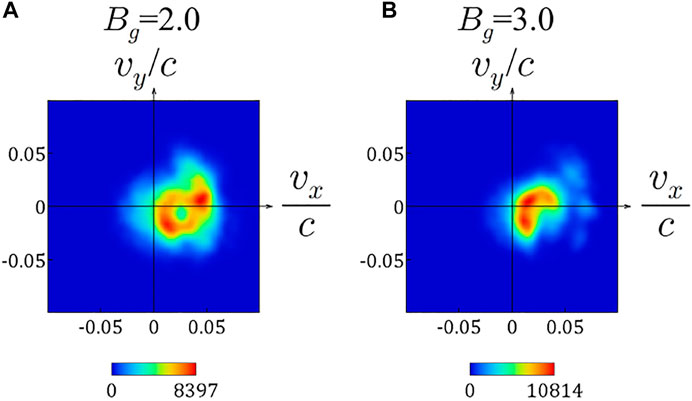
FIGURE 1. Ion velocity distributions obtained by particle simulations in previous works (A): a circle -shaped structure is formed in a B_g = 2.0 case (B): a circular-arc-shaped structure is formed in a B_g = 3.0 case.

Here in short we compare our previous works and this work, and clearly state the difference. In the previous works (Usami et al., 2017; Usami et al., 2019a; Usami et al., 2019b), we have ignored a ring’s width as drawn in Figure 2A. In this work, we consider a ring-shaped velocity distribution with a finite width, as illustrated in Figure 2B.

FIGURE 2

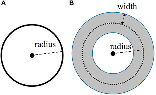
FIGURE 2. Schematic diagrams of (A): a circle, i.e., a ring with no width and (B): an annulus, i.e., a ring with a finite width. Here, the radius of the dotted circle is conventionally regarded as the radius of the annulus.

For the purpose of use in the following theory and simulation, we extend the concept of thermal velocity and temperature to be applicable to non-Maxwellian distributions as effective thermal velocity and effective temperature. We define the effective thermal velocity of j-component v_Teff,j as the standard deviation of particle velocities,

$v_{T\mathrm{e}\mathrm{ff},j}^2=\frac{\int {\left(v_j-⟨v_j⟩\right)}^{2}f{d}^{3}v}{\int f{d}^{3}v},(1)$

where f is a velocity distribution function, v_j represents the j-component of a particle velocity, and ⟨v_j⟩ is the j-component of the averaged velocity. A ring (no matter if it has a width or not) is a two-dimensional structure. Thus, taking, for example, the x- and y-components as the two components in two dimensions, we define the effective thermal velocity of a ring velocity distribution as

$v_{T\mathrm{e}\mathrm{ff}}^2=\frac{1}{2}\left(v_{T\mathrm{e}\mathrm{ff},x}^2+v_{T\mathrm{e}\mathrm{ff},y}^2\right).(2)$

Also, the effective ion temperature is defined as $T_i=m_i{v}_{T\mathrm{e}\mathrm{ff}}^2$, where m_i is the ion mass. In the case of a circle, i.e., a ring with no width as illustrated in Figure 2A, the effective temperature is $1/2m_i{u}_{\text{out}}^2$, where say the radius is u_out. In the case of an annulus, i.e., a ring with a width, as drawn in Figure 2B, the effective temperature is clearly larger than $1/2m_i{u}_{\text{out}}^2$, Here, it is noted that the width has the same length on the both sides of the dotted circle and conventionally the annulus’s radius u_out is defined to be the averaged value of the outer circle’s and the inner circle’s radii.

The width of a ring is caused predominantly by velocity variations of ions entering the downstream, which will be discussed in Section 4.3. In the theories of the previous works, Refs. (Usami et al., 2017), (Usami et al., 2019a), and (Usami et al., 2019b), we have ignored the velocity variations and have supposed that all the ions have the same entry velocity (0, 0). In this work in contrast, we incorporate velocity variations of the entry velocity around (0, 0) into the theory. Here, let us point out an important key point in treatment of the width of a circle. Assuming again the uniform B_z and E_y, the orbits of the ions are circles whose center is (u_out, 0) in the velocity space (u_out = cE_y/B_z). The key point is that the ions have the same gyroperiod, not depending on each ion velocity, while the circle size in the velocity space depends on each ion velocity. It is obvious that as an ion has higher speed perpendicular to the magnetic field, the circumference along which the ion traces is larger. This means that the density in the velocity space is inverse-proportional to the distance from (u_out, 0), if the same number of ions are assigned on each circumference of various concentric circles. We need always to take into account the so-called inverse-proportional effect.

Now we consider a specific case of a ring’s width, in which ions satisfying a Maxwellian velocity distribution $\exp [-(v_x^2+v_y^2)/(2v_{\text{width}}^2)]$ continuously enter the downstream and rotate around the center (u_out, 0) as illustrated in Figure 3A. The velocity distribution newly created in the downstream is a ring with a width, as shown in Figure 3B. The effective thermal speed v_Teff in this case is analytically derived as

$v_{T\mathrm{e}\mathrm{ff}}^2=\frac{1}{2}{u}_{\text{out}}^2+v_{\text{width}}^2.(3)$

FIGURE 3

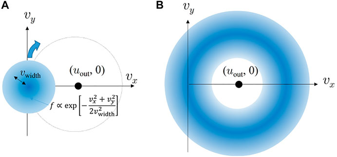
FIGURE 3. Schematic diagrams showing that (A): an initial Maxwellian distribution begins to rotate around the center (u_out, 0) and that (B): a ring-shaped distribution with a width is newly created as a result of the rotation of the initial Maxwellian distribution.

(In Appendix of Ref. (Usami et al., 2019b), we have analyzed a case of a one-dimensional Maxwellian distribution $\exp [-v_x^2/(2v_{\text{width}}^2)]$, where $v_{T\mathrm{e}\mathrm{ff}}^2=1/2u_{\text{out}}^2+1/2v_{\text{width}}^2$ has been derived).

Next, we calculate the new velocity distribution G (v_x, v_y) created as a result of the process that particles satisfying a Maxwellian distribution $\exp [-(v_x^2+v_y^2)/(2v_{\text{width}}^2)]$ are continuously supplied and the particles are rotated once around the point (u_out, 0). The function G (v_x, v_y) is obtained by integrating $\exp [-(v_x^2+v_y^2)/(2v_{\text{width}}^2)]$ on each circumference whose radius is $V=\sqrt{{(v_x-u_{\text{out}})}^2+v_y^2}$ and dividing the value by each circumferential length, because we can interpret the above situation to be equivalent to the following one. Initially a part of the ions were located non-uniformly on a circumference, whose radius is taken to be V. Let these ions be the Group V. If we distribute the ions of the Group V uniformly on the circumference whose radius is V for each value of V (0 < V < ∞), we obtain a new function depending only on V. The new function is G (v_x, v_y) to be derived. Hence, the following equation holds:

$G\left(v_x,v_y\right)=\frac{1}{2\pi V}{\int }_0^{2\pi }\frac{1}{2\pi v_{\text{width}}^2}\exp \left[-\frac{v_x^2+v_y^2}{2v_{\text{width}}^2}\right]Vd\theta .(4)$

By using the polar representation with the center (u_out, 0), v_x = u_out + V cos θ and v_y = V sin θ,

$\begin{array}{ccc}\hfill G\left(v_x,v_y\right)& =\hfill & \frac{1}{{\left(2\pi v_{\text{width}}\right)}^2}\exp \left[-\frac{V^2+u_{\text{out}}^2}{2v_{\text{width}}^2}\right]{\int }_0^{2\pi }\exp \left[-\frac{u_{\text{out}}V}{v_{\text{width}}^2}\cos \theta \right]d\theta ,\hfill \end{array}(5)$

$\begin{array}{ccc}\hfill & =\hfill & \frac{1}{2\pi v_{\text{width}}^2}\exp \left[-\frac{V^2+u_{\text{out}}^2}{2v_{\text{width}}^2}\right]I_0\left(\frac{u_{\text{out}}V}{v_{\text{width}}^2}\right),\hfill \end{array}(6)$

is derived, where I_n is the modified Bessel function of the first kind. It is noted that G (v_x, v_y) is dependent only on V, but G (v_x, v_y) is a probability density function of the velocity vector (v_x, v_y), i.e., G (v_x, v_y) is a distribution function on two-dimensional space (v_x, v_y). On the other hand, by virtue of the axisymmetric structure of G (v_x, v_y), the cross-sections of G (v_x, v_y) have the same profile for any line crossing the center (u_out, 0). In the following discussion, thus, we use the cross-section function of the newly formed distribution

$F\left(v\right)=\frac{1}{2\pi v_{\text{width}}^2}\exp \left[-\frac{v^2+u_{\text{out}}^2}{2v_{\text{width}}^2}\right]I_0\left(\frac{u_{\text{out}}v}{v_{\text{width}}^2}\right),(7)$

where − ∞ < v < ∞.

By analyzing Eq. 7, we show that the shape of the newly formed velocity distribution significantly changes depending on u_out and v_width and derive necessary conditions for the distribution to be a pseudo-Maxwellian distribution. For this purpose, we investigate whether the profile has a dip¹, in other words, a local minimum in the center. It can be said that if F(v) has a dip in the center, it is not a pseudo-Maxwellian distribution, while if F(v) does not have a dip, it is a pseudo-Maxwellian one. We treat F(v) only for v > 0, because F(v) is an even function. We can find that F → 0 for v → ∞ and F monotonically decreases in the regime of v ≫ v_width. Hence, whether F has a dip or not depends on the sign of dF/dv in the vicinity of v = 0. If dF/dv is positive at v ≃ 0, F has a dip. Differentiating F with respect to v, we have

$\frac{dF}{dv}=\exp \left[-\frac{v^2+u_{\text{out}}^2}{2v_{\text{width}}^2}\right]\left[-\frac{v}{v_{\text{width}}^2}{I}_0\left(\frac{u_{\text{out}}v}{v_{\text{width}}^2}\right)+\frac{d{I}_0}{dv}\left(\frac{u_{\text{out}}v}{v_{\text{width}}^2}\right)\right].(8)$

By using formulas of the modified Bessel function of the first kind, dI₀(x)/dx = I₁(x), and the following approximation by Taylor expansion in the vicinity of x = 0, I₀(x) = 1 + (dI₀/dx) (0)x + ⋯ ≃ 1 and I₁(x) = 0 + (dI₁/dx) (0)x + ⋯ ≃ 1/2x, we obtain

$\frac{dF}{dv}\simeq -\exp \left[-\frac{v^2+u_{\text{out}}^2}{2v_{\text{width}}^2}\right]\left(\frac{v}{v_{\text{width}}^4}\right)\left(v_{\text{width}}^2-\frac{1}{2}{u}_{\text{out}}^2\right).(9)$

This equation clearly indicates that if the condition

$v_{\text{width}}>\frac{u_{\text{out}}}{\sqrt{2}},(10)$

is satisfied, dF/dv is negative in the vicinity of v = 0, that is, F does not have a dip in the center. Accordingly, we can expect that the newly created distribution is a pseudo-Maxwellian distribution. In contrast, when $v_{\text{width}}<u_{\text{out}}/\sqrt{2}$, dF/dv is positive in the vicinity of v = 0. The velocity distribution has a dip, and hence a pseudo-Maxwellian distribution is not formed.

In Figure 4, we depict a bird’s eye view of the distribution function G (v_x, v_y) in the left panels and the cross-section function F(v) in the right panels. We set v_width = 0.5, 0.7, and 1.0, for cases of Figures 4A–C, respectively, while we assign u_out = 1.0 for all the cases. In each right panel, the solid line represents F(v), and the dotted line indicates a Maxwellian distribution function which has the standard deviation equal to the one of F(v). In Figure 4A, we can find that the profile has a dip, and thus a ring-shaped distribution holds. In Figure 4B, there is not a dip, but there is a plateau in the center of the profile. This is because v_width is nearly equal to $u_{\text{out}}/\sqrt{2}$ and hence the gradient in the vicinity of the center is nearly equal to zero, as predicted by Eq. 9. In the case of Figure 4C, we can see that the shape becomes a mountain-like structure, which almost fits with a Maxwellian distribution. In what follows, we call such distributions with no dip for $v_{\text{width}}>u_{\text{out}}/\sqrt{2}$ pseudo-Maxwellian velocity distributions. One likely can not distinguish a pseudo-Maxwellian distribution and a genuine-Maxwellian distribution, alone by observing the shapes.

FIGURE 4

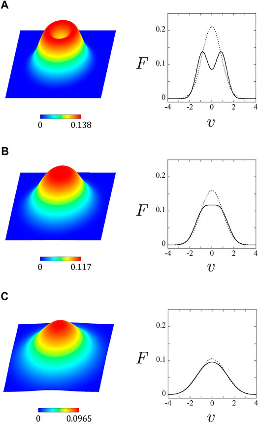
FIGURE 4. The left panels depict a bird’s eye view of the function G (v_x, v_y) and the right panels plot graphs of the function F(v) expressing the cross-section of G (v_x, v_y) (A): v_width = 0.5 (B): v_width = 0.7, and (C): v_width = 1.0 are assigned, while keeping u_out = 1.0.

Lastly in this section, we excuse a slight lack of precision in the discussion of the newly created velocity distribution. This is responsible for complexity in explaining the bridge of the Lagrangian point of view (the individual particle motion) and the Eulerian point of view (the velocity distribution). From the Lagrangian viewpoint, the particle motion is E × B drift while in gyromotion, and the orbits in the velocity space (v_x, v_y) are circles. From the Eulerian viewpoint, we focus on a small local area whose size is much smaller than the Larmor radius of particles whose gyration speed is u_out. Thus, not the entire trajectory of a certain particle is contained inside the small area. We have stated as if the newly formed distribution is composed of the entire orbits of particles, but this physical picture is not correct in a precise sense. The exact physical picture is that the velocity distribution is composed of particles inside a local area at a certain moment, which particles have various gyration phases, because of a mixing of gyration phases. For the sake of convenience, we have described the formation process of a velocity distribution from the Lagrangian point of view, but the essential part of the theory has been maintained.

3 Particle Simulation Method

We search for pseudo-Maxwellian velocity distributions in collisionless driven magnetic reconnection in the presence of a guide magnetic field by means of two-dimensional electromagnetic particle-in-cell (PIC) simulations, using “PASMO” (Horiuchi and Sato, 1997; Pei et al., 2001a; Pei et al., 2001b; Ohtani and Horiuchi, 2009).

In PASMO, an open boundary condition is employed. At the upstream boundary (y = ±y_b), in order to generate plasma inflows and magnetic fluxes, an external driving electric field E_d is imposed in the direction perpendicular to the magnetic field (The terms of “perpendicular” and “parallel” indicate perpendicular and parallel to the magnetic field at each position, not to the averaged or initial magnetic field.) The driving electric field E_d is set to zero at the initial time and begins to grow first near the center of the upstream boundary (x = 0, y = ±y_b). The inflow region where E_d is imposed expands in the ± x directions with a speed of 1.2v_A,up, where v_A,up is the Alfvén speed for the antiparallel magnetic field at the upstream boundary. Eventually E_d develops to reach E_dz = −0.04B_x0 in the entire upstream boundary, where E_dz is the z-component of E_d. As E_d grows, the magnetic field at the upstream boundary rises according to Faraday’s law. In addition, E_x = 0 and ∂E_y/∂y = 0 are applied at the upstream boundary. At the upstream boundary, every time step, all the particles are removed and particles are freshly set which satisfy a shifted Maxwellian velocity distribution, whose averaged velocity is equal to the E × B drift velocity. The plasma density at the upstream boundary is adjusted to be proportional to the magnetic field strength so that the frozen-in constraint holds at the upstream boundary. By this procedure, particles are continuously supplied from the upstream boundary into the simulation domain. In contrast, the downstream boundary (x = ±x_b) is taken to be free, across which particles can freely go in and out. Some technical methods are implemented into PASMO in order for particles with a distribution to continuously and smoothly cross the downstream [for detail, see (Ohtani and Horiuchi, 2009)]. On the following components of the electromagnetic field, the conditions ∂E_x/∂x = ∂B_y/∂x = ∂B_z/∂x = 0 are imposed. The other components of the electromagnetic field are derived by solving Maxwell’s equations at the downstream boundary.

As the initial condition, we take a one-dimensional Harris-type equilibrium with an antiparallel magnetic field in the x direction B_x and a uniform guide magnetic field in the z direction B_z. Thus, the initial state is expressed as

$B_x\left(y\right)=B_{x0}\tanh \left(y/L\right),(11)$

$B_z\left(y\right)=B_{z0},(12)$

$P\left(y\right)=P_0+B_{x0}^2/\left(8\pi \right){\mathrm{s}\mathrm{e}\mathrm{c}\mathrm{h}}^2\left(y/L\right),(13)$

where P represents the plasma pressure. The quantities B_x0, B_z0, and P₀ are constants, and L is a spatial scale in the y-axis. The initial particle velocity distribution is a shifted Maxwellian distribution with spatially uniform temperature. The initial ion temperature is taken to be equal to the initial electron temperature.

The simulation parameters are as follows. The simulation domain size is 2x_b × 2y_b = (15.81 × 2.63)c/ω_pi, where ω_pi is the ion plasma frequency. The plasma frequency is defined by the use of the initial number density at the neutral line y = 0, n₀. The initial number of electrons and the initial number of ions are 28 182 528, respectively. The ion-to-electron mass ratio is taken to be m_i/m_e = 100, i.e., a reduced mass ratio is used (The influence of the mass ratio on the pickup-like process has been discussed in Ref. (Usami et al., 2019b). In a short conclusion, it is theoretically predicted that the pickup-like process works better under the real mass ratio.) The ratio of the electron plasma frequency to the electron gyrofrequency is ω_pe/ω_ce = 6.0, where we define ω_ce = eB_x0/(m_ec). The Alfvén speed for B_x0 and n₀ is v_A0/c = 0.017. The time step is ω_piΔt = 0.0052, and the grid spacing is Δ_g/(c/ω_pi) = 0.010.

4 Particle Simulation Result

4.1 Pseudo-Maxwellian Velocity Distribution

We perform a particle simulation run under the conditions of B_g = B_z0/B_x0 = 1.0, L/(c/ω_pi) = 0.66, and $P_0/(B_{x0}^2/8\pi )=0.35$. In Figures 5A–C, we display simulation results in the region of −5.27 < x/(c/ω_pi) < 5.27 at ω_pit = 775 and in Figure 5D we show a simulation result at the initial time, where the electromagnetic field, the velocity, and the temperature are normalized to B_x0, c, and m_ec², respectively. By ω_pit = 775 the reconnection electric field is balanced with the driving electric field E_dz imposed at the upstream boundary, and the reconnection system is in a quasi-steady state. Figure 5A shows the spatial profile of the out-of-plane component of the magnetic field B_z as color contours and magnetic field lines. Magnetic reconnection is driven by plasma inflows and magnetic fluxes supplied from the upstream boundary, and the reconnection point, the X-point, is located at the center of the simulation domain (0, 0). The out-of-plane component of the magnetic field consists of the initial guide field B_z0 and the quadrupole magnetic field generated by the Hall current. As a result, B_z is positive in the main part of the downstream, although B_z is negative in small parts. Figure 5B shows the ion bulk velocity vectors as arrows and the y-component of the electric field E_y as color contours. From the velocity vectors, we can see that bipolar reconnection outflows emanate from the X-point, and from the E_y profile, we can find that E_y is produced in the entire downstream as the dominant component of the convective electric field. Figures 5C,D depict the spatial profiles of the ion temperature perpendicular to the magnetic field T_i⊥ at ω_pit = 775 and at ω_pit = 0, respectively. It is clearly seen that the ion temperature rises mainly in the downstream at ω_pit = 775, comparing Figure 5C with Figure 5D.

FIGURE 5

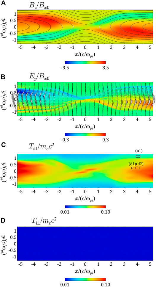
FIGURE 5. Spatial profiles of (A): B_z and the magnetic field lines (B): the ion bulk velocity vectors and E_y (C) and (D): the ion temperature perpendicular to the magnetic field. The panels (A)–(C) display results at ω_pit = 775, and the panel (D) shows a result at the initial time.

In Figures 6A,B, we show ion velocity distributions taken at the boxed areas (d1) and (d2) designated in Figure 5C, respectively. Unlike the cases of B_g = 2.0 and 3.0 introduced in Figure 1, we can see that instead of a circle-shaped or an arc-shaped structure, mountain-shaped velocity distributions, which are the central part near (v_x, v_y) = (0, 0), are formed. These velocity distributions are too similar to a Maxwellian distribution to be distinguishable in shape, and thus we interpret them to be pseudo-Maxwellian distributions as described in Section 2. Here, Figure 6 indicates that an additional structure is attached to the right part of each pseudo-Maxwellian distribution. It is a horn-shaped distribution discussed in Ref. (Usami et al., 2019a), which is a kind of circular-arc-shaped velocity distribution. The formation process of horn-shaped velocity distributions is explained by an extended theory of the pickup-like process. For details, refer to Ref. (Usami et al., 2019a).

FIGURE 6

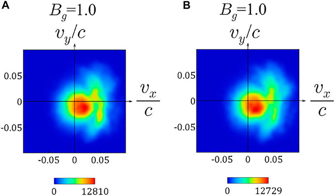
FIGURE 6. Ion velocity distributions (A): in the boxed area (d1) and (B): in the boxed area (d2) indicated in Figure 5C. In both panels, pseudo-Maxwellian distributions are seen at the central part near (v_x, v_y) = (0, 0).

We almost conclude that the mountain-like distributions shown in Figure 6 are pseudo-Maxwellian distributions, i,e., ring-shaped distributions with an extremely large width, based on the existing of an additional horn-shaped structure, which also is created by the pickup-like process. However, an intriguing property of the pseudo-Maxwellian distributions, that the shape is quite similar to the genuine-Maxwellian shape, acts as a negative aspect, when rigorously determining whether a mountain-like distribution is a pseudo-Maxwellian or a genuine-Maxwellian distribution in particle simulations. Although pseudo-Maxwellian and genuine-Maxwellian distributions are theoretically expressed by obviously different functions, it is practically impossible for particle simulations to directly detect the deference so as to distinguish the two. In particle (particle-in-cell) simulations, including PASMO, employing the super-particle method (Birdsall and Langdon, 1991), the number of particles are much less than that in actual plasmas. Thus, statistical fluctuations are inevitably contained in velocity distributions. In addition, other physical effects could affect the shape of velocity distributions for this case, which will be shortly described in Section 6. Accordingly, alone by using the simulation results shown in Section 4.1, we can not completely deny that the distributions shown in Figure 6 might be genuine-Maxwellian distributions. In Section 4.2 and in Section 5, we demonstrate two kinds of evidence to conclude that the distributions in Figure 6 are pseudo-Maxwellian distributions, and furthermore to lead to implication that pseudo-Maxwellian distributions would be frequently formed in some cases of magnetic reconnection with a guide field.

4.2 Guide Field Dependence (Evidence 1)

In order to more definitely demonstrate that the distributions found in Figure 6 are pseudo-Maxwellian distributions, we carry out a series of particle simulations and investigate the dependence of the shape of ion velocity distributions on the guide magnetic field. We show velocity distributions in the (v_x, v_y) plane and in the $(v_{\tilde{x}},v_{\tilde{y}})$ plane, where $\tilde{x}$ and $\tilde{y}$ are two directions which are mutually perpendicular and are perpendicular to the magnetic field. The reason is as follows. If a ring-shaped velocity distribution is formed, it is clearly observed in the $(v_{\tilde{x}},v_{\tilde{y}})$ plane, because a ring is created as a result of the gyration. If the out-of-plane component of the magnetic field is dominant, the (x, y) plane is nearly perpendicular to the magnetic field so that the (v_x, v_y) plane is almost equal to the $(v_{\tilde{x}},v_{\tilde{y}})$ plane. In Refs. (Usami et al., 2017) and (Usami et al., 2019b), we have displayed velocity distributions in the (v_x, v_y) plane for cases of high guide-field such as B_g = 2–4. In this work, however, we show results mainly for B_g = 1–2, and thus add velocity distributions in the $(v_{\tilde{x}},v_{\tilde{y}})$ plane. Let us define $v_{\tilde{x}}=\mathit{v}\cdot ({\mathit{E}}_{\perp }\times \mathit{B})/(E_{\perp }B)$, $v_{\tilde{y}}=\mathit{v}\cdot {\mathit{E}}_{\perp }/E_{\perp }$, and $v_{\tilde{z}}=\mathit{v}\cdot \mathit{B}/B$, where E_⊥ is the perpendicular component of E to B, i.e., E_⊥ = E − [E⋅B/B]B/B.

Figures 7A–D show ion velocity distributions for cases of B_g = 1.2, 1.4, 1.6, and 1.8, respectively. The upper and lower panels represent velocity distributions in the (v_x, v_y) plane and in the $(v_{\tilde{x}},v_{\tilde{y}})$ plane, respectively. The locations of the area for the panels (A)-(D) are the same as the one for Figure 6B. It is found from the panel (A) that a ring-shaped structure is not seen, but a mountain-like structure is seen in the case of B_g = 1.2. In contrast, according to the panels (B)-(D), as B_g is larger, we can observe a clearer ring. To quantify the clearness of rings, we extract each one-dimensional profile along the v_y-axis crossing the center of a mountain or a ring from the panels (A)-(D) and obtain each best-fit Gaussian (Maxwellian distribution) curve based on regression analysis. The values of the coefficient of determination R² for the panels (A)-(D) are 0.987, 0.952, 0.945, and 0.889, respectively, which indicates that the shape is close to the Maxwellian function in the order of (A) (B) (C), and (D). It can be said that the clearness of rings is in the order of (D) (C) (B), and (A). Next, we can find that the rings are clear in the $(v_{\tilde{x}},v_{\tilde{y}})$ plane, compared with in the (v_x, v_y) plane, as we predict. From the velocity distributions seen in the $(v_{\tilde{x}},v_{\tilde{y}})$ plane, we can surely grasp that ring-shaped structures are formed only for B_g = 1.4, 1.6, and 1.8. (Note that horn-shaped distributions overlap ring-shaped or pseudo-Maxwellian structures. As a consequence, the density is extensively increased only in the overlapping part. If the upper limit of the color contours is taken to be the maximum value for each panel as displayed in Figure 7, the ring sharpness is no longer in the order of the panel (D) (C) and (B), which leads to misunderstanding. We, therefore, use a common upper limit among the upper panels and a common upper limit among the lower panels, respectively.)

FIGURE 7

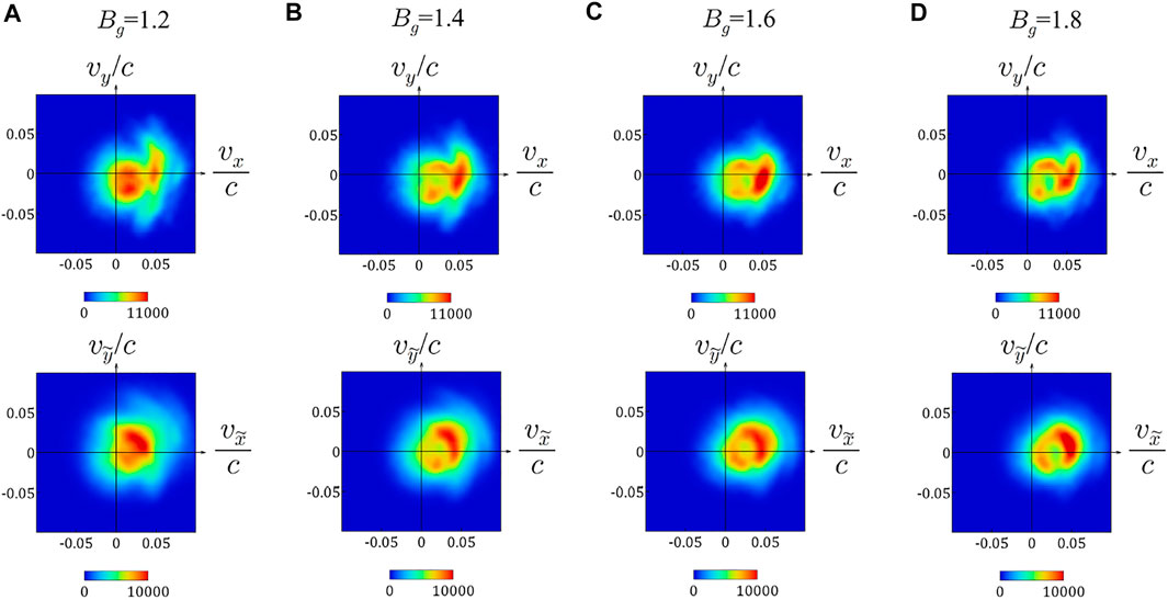
FIGURE 7. Ion velocity distributions for various values of the guide field ratio B_g (A): B_g = 1.2 (B): B_g = 1.4 (C): B_g = 1.6, and (D): B_g = 1.8. The upper panels are taken in the (v_x, v_y) plane, and the lower panels are taken in the $(v_{\tilde{x}},v_{\tilde{y}})$ plane.

Described from the opposite viewpoint, as B_g is decreased, the ring-shaped structure gradually becomes ambiguous. In other words, it is not sudden that the ring disappears when B_g = 1.0. Hence, the following interpretation is plausible. The pickup-like ion motion, which forms a ring-shaped velocity distribution, does work for B_g = 1.0. In Figure 6, rings exist, but the width is so large that the dip of the ring’s center is plugged and the peak of a mountain is formed in the center. Therefore in conclusion, the velocity distributions in Figure 6 are pseudo-Maxwellian distributions.

4.3 Physics of a Ring’s Width

We discuss what kind of process causes the width of ring-shaped velocity distributions. The initial thermal velocity surely plays a role, and in addition it is believed that compressional heating inside the upstream predominantly contributes to the formation of a ring’s width. In what follows, we demonstrate that v_width corresponds to (genuine) thermal velocity in the upstream v_T,up, which depends on the guide magnetic field. In the following description, we use Eq. 10 substituting v_T,up into v_width.

Let us compare the spatial profiles of the ion temperature at ω_pit = 775 and at the initial time in Figures 5C,D. We can see that at ω_pit = 775, the ion temperature is increased not only in the downstream but also in the upstream, although the temperature increment in the upstream is much less than that in the downstream. Figures 8A,B show ion velocity distributions at ω_pit = 775 and at the initial time, respectively, in the boxed area (u1), which is in the upstream. In both cases, Maxwellian distributions are satisfied, while the thermal speed is clearly larger at ω_pit = 775 than that at the initial time. This indicates that in terms of fluid dynamics, compressional heating occurs in the upstream, because plasmas and magnetic fluxes are continuously injected from the upstream in our particle simulations. Furthermore, in Figure 8C we depict an ion velocity distribution at the same position at ω_pit = 775 in a case of B_g = 2.0. Comparing Figures 8A,C, we can find that the ion thermal speed for B_g = 2.0 is smaller than that for B_g = 1.0. In the upstream, the ion thermal speed is $\sqrt{B_{\mathrm{u}\mathrm{p}}/B_0}$ times larger than the initial one, where B_up and B₀ are the magnetic field at a certain time and at the initial time, because the conservation of the magnetic moment approximately holds. Thus, we infer that as the initial magnetic field B_z0 is larger, that is, as the guide magnetic field is larger, the compressional heating tends to be weaker.

FIGURE 8

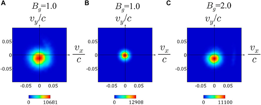
FIGURE 8. Ion velocity distributions (A): in the boxed area (u1) designated in Figure 5C at ω_pit = 775 for B_g = 1.0 (B): at the initial time, and (C): in the area (u1) at ω_pit = 775 for a different simulation run of B_g = 2.0.

In Figure 9, we plot the values of the ion thermal speed in the upstream v_T,up (the blue solid line) and the reconnection outflow speed u_out (the black solid line) observed in the particle simulations for various values of B_g. In order to refer to velocity distributions in the areas (d1) and (d2) of Figure 5C, we observe the value of u_out around the areas (d1) and (d2), because the outflow speed depends to some extent on the position in the downstream. Here, we regard that u_out is the x-component of the ion bulk velocity averaged over the region of 3.5 < x/(c/ω_pi) < 5.0 and 0.0 < y/(c/ω_pi) < 0.5 inside the downstream, and as v_T,up we use the ion thermal velocity averaged over the region of |x/(c/ω_pi)| < 6.0 and |y/(c/ω_pi)| > 1.0 inside the upstream. As B_g is larger, v_T,up becomes smaller. In contrast, as B_g is larger, u_out become larger, because the change in B_g affects the density and the reconnection magnetic field in the upstream. For comparison, we plot $u_{\text{out}}/\sqrt{2}$ as the black dashed line. When B_g = 1.0, v_T,up is greater than $u_{\text{out}}/\sqrt{2}$, and when B_g = 1.2, v_T,up is very close to $u_{\text{out}}/\sqrt{2}$, although v_T,up is slightly less than $u_{\text{out}}/\sqrt{2}$. Hence, as shown in Figure 6 and Figure 7A, ring-shaped velocity distributions are not seen. In contrast, because $v_{T,\mathrm{u}\mathrm{p}}<u_{\text{out}}/\sqrt{2}$ is sufficiently satisfied for B_g > 1.4, we can see ring-shaped velocity distributions, as shown in Figures 7B–D.

FIGURE 9

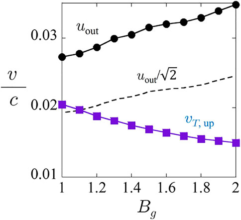
FIGURE 9. Reconnection outflow velocity u_out (the black solid line) and ion thermal velocity in the upstream v_T,up (the blue solid line) for various values of the guide field ratio B_g. For comparison, $u_{\text{out}}/\sqrt{2}$ (the black dashed line) is added.

5 Test Particle Simulation (Evidence 2)

In order to further prove that the mountain structures shown in Figure 6 are rings with a large width, i.e., pseudo-Maxwellian distributions, we perform a test particle simulation (Usami et al., 2019a). The method of the test particle simulation is as follows. Before the test particle simulation, we perform a particle simulation run by using the above particle simulation model, PASMO and obtain data of an electromagnetic field at some instant, which corresponds to magnetic reconnection in a quasi-steady state. In the test particle simulation, the equations of motion for test particles are solved in the electromagnetic field given by the particle simulation. In the following run of the test particle simulation, as the given field, we use the electromagnetic field at ω_pit = 775 for B_g = 1.0, as displayed in Figures 5A,B.

We demonstrate the positions of the ion particles at various times (A) ω_piτ = 0 (B) 90, and (C) 240 in Figure 10. For distinguishing the time in the test particle simulation from the time in the particle simulations, we use τ as the time in the test particle simulation. The panel (A) shows that the test ions are set in the area of 0 < x/(c/ω_pi) < 7.91 on the upstream boundary y/(c/ω_pi) = ±1.31. The number of test ions is 60 000, and we set 30 000 ions on the line y/(c/ω_pi) = 1.31 and 30 000 ions on the line y/(c/ω_pi) = −1.31. Initially, each test ion is set to have a velocity equal to the ion fluid velocity at each position. At ω_piτ = 90 (the panel (B)), the ions have entered the downstream from the upper- and lower-sides of the upstream boundary. After that, the ions move in the x direction, and then at ω_piτ = 240 (the panel (C)), some ions have already escaped from the simulation domain across the downstream boundary x/(c/ω_pi) = 7.91. The test particle simulation run is terminated at ω_piτ = 300.

FIGURE 10

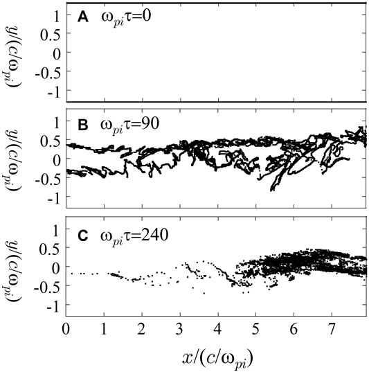
FIGURE 10. Positions of the ions calculated by a test particle simulation (A): at ω_piτ = 0 (B): at ω_piτ = 90, and (C): at ω_piτ = 240.

Under a steady state of reconnection, particles continuously flow inward from the upstream with a constant flux. In the test particle simulation, however, we do not assign new particles at the upstream boundary after the initial time. Instead of a continuous supply of particles, we accumulate the temporal sequence data of the particles during ω_piτ = 0–300 in order to mimic particles continuously supplied under a steady state. Thus, when we plot the velocities of particles in Figure 11, we display not only the particles which are in a certain area at the instance of ω_piτ = 300, but the particles which were and are in the area by ω_piτ = 300. We record the particle data every ω_piΔτ = 3, and treat an identical particle at a past time as a different particle. This means that some particles are displayed in Figure 11 multiple times.

FIGURE 11

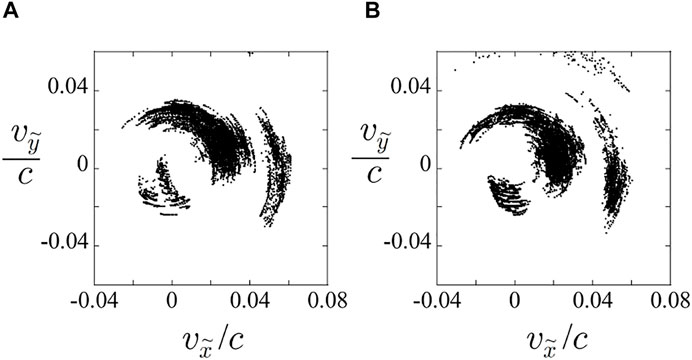
FIGURE 11. Velocities $(v_{\tilde{x}},v_{\tilde{y}})$ of the ions inside small areas whose locations are the same as (A): the boxed area (d1) and (B): the boxed area (d2) represented in Figure 5C, respectively.

The fact that the test ions have initial velocities equal to the ion fluid velocity means that ions with zero temperature are hypothetically set. Consequently, we can significantly reduce the ring’s width v_width. In Figures 11A,B, we plot velocities $(v_{\tilde{x}},v_{\tilde{y}})$ of the ions inside the boxed areas (d1) and (d2) designated in Figure 5C, where the velocity distributions in Figure 6 are observed. In the both cases, we can clearly see a ring-shaped structure (with an additional horn-shaped structure), which can not be seen by means of particle simulations.

On the basis of the result that in a test particle simulation run for B_g = 1.0, ring-shaped structures are created at the positions corresponding to Figure 6, we can derive a plausible interpretation as follows. In the velocity distributions shown in Figure 6, ring-shaped structures with a finite width surely exist, but the width is so large that they are observed as pseudo-Maxwellian distributions. Therefore, it is definitely confirmed that the velocity distributions of Figure 6 are pseudo-Maxwellian distributions.

6 Discussion and Suggestion

As we described in Section 5, we hypothetically treat cold ions with zero temperature in the test particle simulation run, by assigning the initial velocities equal to the ion fluid velocity at each position. Nevertheless, the ring-shaped structures shown in Figure 11 have a finite width. The fluid velocity slightly depends on the position in the upstream boundary, and ions which exist in a small area of the downstream are ones which have come from different positions in the upstream. Hence, the ions in a small area of the downstream have slightly different velocities, which contribute to the width of a ring. In addition, if some adiabatic ions, which are not responsible for the pickup-like process, exist, they will affect the shape of a velocity distribution. Furthermore, the electromagnetic field is not completely uniform in the downstream. This non-uniformity enhances variation of ion velocities. Chaotic motions of ions might play a role in producing variations of their velocities (Zenitani et al., 2017). These topics are beyond the current work, and will be discussed as a future work.

Let us suggest that pseudo-Maxwellian distributions would have been misidentified as genuine-Maxwellian distributions in particle simulations and satellite observations, since the two kinds of distributions are almost indistinguishable in shape from each other. A pseudo-Maxwellian velocity distribution is a kind of ring-shaped distribution, and it is an indicator showing that particles behave as nonadiabatic and are effectively heated through the pickup or the pickup-like process. Although effective heating events by the pickup or the pickup-like process occur in various situations more frequently or more universally than expected, they would have been overlooked so far.

Though the motivation of the present work stems from magnetic reconnection, the application of the theory of the pseudo-Maxwellian distribution will not be limited to magnetic reconnection. Let us generalize the situation as follows. Seed charged particles satisfy shifted Maxwellian distribution $\exp [-{(\mathit{v}-{\mathit{v}}_d)}^2/(2v_{T0}^2)]$, and the seed particles are continuously supplied to a region where a magnetic field B and an electric field E are imposed. Under this generalized situation, u_out on the right-hand side of Eq. 10 should be the relative velocity between the averaged velocity of the seed particles and the E × B drift velocity in the region. We do not need the existence of a plasma flow corresponding to the reconnection outflow, and all we need is E and B causing E × B drift motion. Based on the above arguments, we can derive the necessary condition to pseudo-Maxwellian distributions as

$v_{T0}>\frac{1}{\sqrt{2}}\left|\frac{cE\times B}{B^2}-{\mathit{v}}_{d\perp }\right|,(14)$

where v_d⊥ is the perpendicular component of v_d to B, i.e., v_d⊥ = v_d − [v_d ⋅B/B]B/B. The effective thermal velocity for the newly created velocity distribution is

$v_{T\mathrm{e}\mathrm{ff}}^2=\frac{1}{2}{\left(\frac{cE\times B}{B^2}-{\mathit{v}}_{d\perp }\right)}^2+{\mathit{v}}_{T0}^2.(15)$

7 Summary

By means of theory and simulations, we have explored the feature of a ring-shaped velocity distribution with a finite width, which is newly formed as a result of the pickup-like process during magnetic reconnection in the presence of a guide magnetic field.

On the basis of a steady feeding of particles which satisfy a Maxwellian velocity distribution and a mixing of gyration phases, we have analytically derived a function which exactly expresses rings with a finite width. Moreover, the formulated function indicates that if the width is larger than $1/\sqrt{2}$ of the radius, the dip of a ring’s center, i.e., the central local minimum is transformed into the peak of a mountain shape, i.e., the maximum. The mountain-like velocity distribution is almost indistinguishable in shape from a Maxwellian velocity distribution. We have named such a distribution a pseudo-Maxwellian distribution.

We have carried out particle simulations of magnetic reconnection with a guide magnetic field, and demonstrated that mountain-like velocity distributions of ions are formed in the downstream. On the basis of the existing of additional horn-shaped distributions, which is a signature showing that the pickup-like process does work, we have almost concluded that the mountain-like distributions are pseudo-Maxwellian velocity distributions. Alone by the above results, however, we could not completely disprove that they are genuine-Maxwellian, because the pseudo-Maxwellian and genuine-Maxwellian distributions are almost indistinguishable in shape from each other.

Hence, we have shown two types of evidence for pseudo-Maxwellian distributions. First, we have clarified the dependence of velocity distributions on the guide magnetic field, by performing a series of particle simulation runs. It has been found that as the guide field is larger, a ring-shaped structure with a finite width gradually becomes clearer in velocity distributions. It is because a ring’s width, which is caused by velocity variations mainly due to the genuine thermal speed in the upstream, and the ring’s radius, which corresponds to the reconnection outflow speed, depend on the guide field. Next, we have performed a test particle simulation, in which the motions of test ion particles with an artificial zero temperature are calculated in an electromagnetic field given by a particle simulation run. The artificial zero temperature considerably contributes to reducing the ring width. As the given field, we have employed one which has formed mountain-like velocity distributions in the particle simulation run. In the test particle simulation, we have observed clear structures of ring-shaped velocity distributions, which have not been seen in the particle simulation run. From the two types of evidence, it has been confirmed that the mountain-like velocity distributions found in the particle simulations are pseudo-Maxwellian distributions. Furthermore, the findings suggest that pseudo-Maxwellian distributions would be formed in various cases of magnetic reconnection with a guide field.

Data Availability Statement

The raw data supporting the conclusions of this article will be made available by the authors, without undue reservation.

Author Contributions

SU constructed the theory, carried out particle simulations and test particle simulations by using supercomputers, analyzed the simulation data, and wrote the paper. RH developed and improved the simulation code “PASMO,” and revised the manuscript.

Funding

This work was supported by JSPS KAKENHI (Grant Numbers 16K17847, 15H05750, 20H00136), the General Coordinated Research at the National Institute for Fusion Science (NIFS21KNSS154), “Joint Usage/Research Center for Interdisciplinary Large-scale Information Infrastructures,” and “High Performance Computing Infrastructure” in Japan (Project ID: jh210005-NAH).

Conflict of Interest

The authors declare that the research was conducted in the absence of any commercial or financial relationships that could be construed as a potential conflict of interest.

Publisher’s Note

All claims expressed in this article are solely those of the authors and do not necessarily represent those of their affiliated organizations, or those of the publisher, the editors, and the reviewers. Any product that may be evaluated in this article, or claim that may be made by its manufacturer, is not guaranteed or endorsed by the publisher.

Acknowledgments

One of the authors (SU) appreciates advice from S. Zenitani so as to construct the theory in Section 2. This simulation work was performed on the supercomputers “Plasma Simulator” (NEC SX-Aurora TSUBASA) at the National Institute for Fusion Science, Japan and “Flow” (FUJITSU PRIMEHPC FX1000) at the Information Technology Center, Nagoya University, Japan.

Footnotes

¹If v_width = 0, F = 0 at v = 0, and the ring center is “a hole.” In genera cases of v_width ≠ 0, F > 0 at v = 0, and thus we call the ring center “a dip.”

References

Ashour-Abdalla, M., and Kennel, C. F. (1978). Nonconvective and Convective Electron Cyclotron Harmonic Instabilities. J. Geophys. Res. 83, 1531–1543. doi:10.1029/JA083iA04p01531

CrossRef Full Text | Google Scholar

Bessho, N., Chen, L. J., and Hesse, M. (2016). Electron Distribution Functions in the Diffusion Region of Asymmetric Magnetic Reconnection. Geophys. Res. Lett. 43, 1828–1836. doi:10.1002/2016GL067886

CrossRef Full Text | Google Scholar

Birdsall, C. K., and Langdon, A. B. (1991). Plasma Physics via Computer Simulation. London: IoP Publishing Ltd.

Google Scholar

Burch, J. L., Torbert, R. B., Phan, T. D., Chen, L.-J., Moore, T. E., Ergun, R. E., et al. (2016). Electron-scale Measurements of Magnetic Reconnection in Space. Science 352, aaf2939. doi:10.1126/science.aaf2939

PubMed Abstract | CrossRef Full Text | Google Scholar

Cheng, C. Z., Inoue, S., Ono, Y., and Horiuchi, R. (2015). Physical Processes of Driven Magnetic Reconnection in Collisionless Plasmas: Zero Guide Field Case. Phys. Plasmas 22, 101205. doi:10.1063/1.4932337

CrossRef Full Text | Google Scholar

Drake, J. F., Cassak, P. A., Shay, M. A., Swisdak, M., and Quataert, E. (2009). A Magnetic Reconnection Mechanism for Ion Acceleration and Abundance Enhancements in Impulsive Flares. ApJ 700, L16–L20. doi:10.1088/0004-637X/700/1/L16

CrossRef Full Text | Google Scholar

Drake, J. F., and Swisdak, M. (2014). The Onset of Ion Heating during Magnetic Reconnection with a strong Guide Field. Phys. Plasmas 21, 072903. doi:10.1063/1.4889871

CrossRef Full Text | Google Scholar

Hesse, M., Norgren, C., Tenfjord, P., Burch, J. L., Liu, Y.-H., Chen, L.-J., et al. (2018). On the Role of Separatrix Instabilities in Heating the Reconnection Outflow Region. Phys. Plasmas 25, 122902. doi:10.1063/1.5054100

CrossRef Full Text | Google Scholar

Horiuchi, R., and Sato, T. (1997). Particle Simulation Study of Collisionless Driven Reconnection in a Sheared Magnetic Field. Phys. Plasmas 4, 277–289. doi:10.1063/1.872088

CrossRef Full Text | Google Scholar

Horiuchi, R., Usami, S., Moritaka, T., and Ono, Y. (2019). Particle Simulation Studies of Merging Processes of Two Spherical-tokamak-type Plasmoids. Phys. Plasmas 26, 092101. doi:10.1063/1.5104281

CrossRef Full Text | Google Scholar

Inomoto, M., Ushiki, T., Guo, X., Sugawara, T., Kondo, K., Mihara, T., et al. (2019). Effects of Reconnection Downstream Conditions on Electron Parallel Acceleration during the Merging Start-Up of a Spherical Tokamak. Nucl. Fusion 59, 086040. doi:10.1088/1741-4326/ab1e0f

CrossRef Full Text | Google Scholar

Ishizawa, A., and Horiuchi, R. (2005). Suppression of Hall-Term Effects by Gyroviscous Cancellation in Steady Collisionless Magnetic Reconnection. Phys. Rev. Lett. 95, 045003. doi:10.1103/PhysRevLett.95.045003

PubMed Abstract | CrossRef Full Text | Google Scholar

Mithaiwala, M., Rudakov, L., and Ganguli, G. (2010). Stability of an Ion-Ring Distribution in a Multi-Ion Component Plasma. Phys. Plasmas 17, 042113. doi:10.1063/1.3372842

CrossRef Full Text | Google Scholar

Möbius, E., Hovestadt, D., Klecker, B., Scholer, M., Gloeckler, G., and Ipavich, F. M. (1985). Direct Observation of He+ Pick-Up Ions of Interstellar Origin in the Solar Wind. Nature 318, 426–429. doi:10.1038/318426a0

CrossRef Full Text | Google Scholar

Ohtani, H., and Horiuchi, R. (2009). Open Boundary Condition for Particle Simulation in Magnetic Reconnection Research. Plasma Fusion Res. 4, 024. doi:10.1585/pfr.4.024

CrossRef Full Text | Google Scholar

Ono, Y., Inoue, S., Tanabe, H., Cheng, C. Z., Hara, H., and Horiuchi, R. (2019). Reconnection Heating Experiments and Simulations for Torus Plasma Merging Start-Up. Nucl. Fusion 59, 076025. doi:10.1088/1741-4326/ab14a4

CrossRef Full Text | Google Scholar

Pei, W., Horiuchi, R., and Sato, T. (2001). Ion Dynamics in Steady Collisionless Driven Reconnection. Phys. Rev. Lett. 87, 235003. doi:10.1103/PhysRevLett.87.235003

PubMed Abstract | CrossRef Full Text | Google Scholar

Pei, W., Horiuchi, R., and Sato, T. (2001). Long Time Scale Evolution of Collisionless Driven Reconnection in a Two-Dimensional Open System. Phys. Plasmas 8, 3251–3257. doi:10.1063/1.1375150

CrossRef Full Text | Google Scholar

Pucci, F., Usami, S., Ji, H., Guo, X., Horiuchi, R., Okamura, S., et al. (2018). Energy Transfer and Electron Energization in Collisionless Magnetic Reconnection for Different Guide-Field Intensities. Phys. Plasmas 25, 122111. doi:10.1063/1.5050992

CrossRef Full Text | Google Scholar

Tanabe, H., Tanaka, H., Cao, Q., Cai, Y., Akimitsu, M., Ahmadi, T., et al. (2021). Global Ion Heating/transport during Merging Spherical Tokamak Formation. Nucl. Fusion 61, 106027. doi:10.1088/1741-4326/ac217c

CrossRef Full Text | Google Scholar

Tanabe, H., Yamada, T., Watanabe, T., Gi, K., Inomoto, M., Imazawa, R., et al. The MAST Team (2017). Investigation of Merging/reconnection Heating during Solenoid-free Startup of Plasmas in the MAST Spherical Tokamak. Nucl. Fusion 57, 056037. doi:10.1088/1741-4326/aa6608

CrossRef Full Text | Google Scholar

Thorne, R. M., and Summers, D. (1989). Kinetic Instability of a Gyrating Ring Distribution with Application to Satellite Pickup in Planetary Magnetospheres. Planet. Space Sci. 37, 535–544. doi:10.1016/0032-0633(89)90094-9

CrossRef Full Text | Google Scholar

Usami, S., Horiuchi, R., and Ohtani, H. (2017). Effective Heating of Nonadiabatic Protons in Magnetic Reconnection with a Guide Field. Phys. Plasmas 24, 092101. doi:10.1063/1.4997453

CrossRef Full Text | Google Scholar

Usami, S., Horiuchi, R., and Ohtani, H. (2019). Horn-Shaped Structure Attached to the Ring-Shaped Ion Velocity Distribution during Magnetic Reconnection with a Guide Field. Plasma Fusion Res. 14, 3401137. doi:10.1585/pfr.14.3401137

CrossRef Full Text | Google Scholar

Usami, S., Horiuchi, R., Ohtani, H., Ono, Y., Inomoto, M., and Tanabe, H. (2019). Dependence of the Pickup-like Ion Effective Heating on the Poloidal and Toroidal Magnetic fields during Magnetic Reconnection. Phys. Plasmas 26, 102103. doi:10.1063/1.5099423

CrossRef Full Text | Google Scholar

Winske, D., and Daughton, W. (2012). Generation of Lower Hybrid and Whistler Waves by an Ion Velocity Ring Distribution. Phys. Plasmas 19, 072109. doi:10.1063/1.4736983

CrossRef Full Text | Google Scholar

Wu, C. S., and Davidson, R. C. (1972). Electromagnetic Instabilities Produced by Neutral-Particle Ionization in Interplanetary Space. J. Geophys. Res. 77, 5399–5406. doi:10.1029/JA077i028p05399

CrossRef Full Text | Google Scholar

Wu, C. S., Yoon, P. H., and Freund, H. P. (1989). A Theory of Electron Cyclotron Waves Generated along Auroral Field Lines Observed by Ground Facilities. Geophys. Res. Lett. 16, 1461–1464. doi:10.1029/GL016i012p01461

CrossRef Full Text | Google Scholar

Yamada, M. (2007). Progress in Understanding Magnetic Reconnection in Laboratory and Space Astrophysical Plasmas. Phys. Plasmas 14, 058102. doi:10.1063/1.2740595

CrossRef Full Text | Google Scholar

Yamada, M., Yoo, J., Jara-Almonte, J., Ji, H., Kulsrud, R. M., and Myers, C. E. (2014). Conversion of Magnetic Energy in the Magnetic Reconnection Layer of a Laboratory Plasma. Nat. Commun. 5, 4774. doi:10.1038/ncomms5774

PubMed Abstract | CrossRef Full Text | Google Scholar

Yoon, Y. D., and Bellan, P. M. (2021). How Hall Electric fields Intrinsically Chaotize and Heat Ions during Collisionless Magnetic Reconnection. Phys. Plasmas 28, 022113. doi:10.1063/5.0040374

CrossRef Full Text | Google Scholar

Zenitani, S., Hasegawa, H., and Nagai, T. (2017). Electron Dynamics Surrounding the X Line in Asymmetric Magnetic Reconnection. J. Geophys. Res. Space Phys. 122, 7396–7413. doi:10.1002/2017JA023969

CrossRef Full Text | Google Scholar

Zenitani, S., and Nagai, T. (2016). Particle Dynamics in the Electron Current Layer in Collisionless Magnetic Reconnection. Phys. Plasmas 23, 102102. doi:10.1063/1.4963008

CrossRef Full Text | Google Scholar