Listening to the Magnetosphere: How Best to Make ULF Waves Audible

1 Introduction

Ultra-low frequency (ULF) waves, with periods between seconds and tens of minutes, provide a mechanism for solar wind energy and momentum to be transferred into/around a planetary magnetosphere and couple the space environment to the body’s ionosphere. They are routinely recorded as time-series data both by ground-based instruments such as magnetometers or radar, as well as through in situ spacecraft observations of the magnetospheric environment. Dynamic pressure variations, either embedded in the large-scale solar wind or associated with meso-scale kinetic structures at the bow shock, may excite any of the three magnetohydrodynamic (MHD) waves—the surface, fast magnetosonic, and Alfvén modes—at locations within the magnetosphere (e.g. Sibeck et al., 1989; Hartinger et al., 2013). In addition, MHD or other plasma waves in the ULF range—such as electromagnetic ion cyclotron (EMIC) and mirror modes—may also be generated internally through fluid/kinetic instabilities or wave-particle interactions (e.g. Cornwall, 1965; Southwood et al., 1969; Hasegawa, 1975). All of these different waves may exist as incoherent broadband enhancements in wave power or at well-defined discrete, or even an entire spectrum, of coherent oscillations. Thus a zoo of ULF wave phenomena are known to occur within Earth’s magnetosphere (see the review of Nakariakov et al., 2016, for more).

Classification of magnetospheric ULF waves (Jacobs et al., 1964) has long been separated into whether pulsations qualitatively are quasi-sinusoidal (continuous pulsations, Pc) or more irregular (Pi). These two categories have then be subdivided into near-logarithmically spaced frequency bands. Unfortunately, such a classification scheme does not take into account the physical processes involved in the generation and propagation of the waves, nor how these may be reflected in their physical or morphological properties. Indeed, many studies simply consider the integrated power over one or several of these frequency bands (e.g. Mann et al., 2004), which will not distinguish between broadband, narrowband, or multi-harmonic signals. It is known, however, that the frequencies of physically different ULF waves may overlap and even occupy wildly different bands depending on the conditions present (e.g. Archer et al., 2015, 2017).

Beyond classification, even the analysis of ULF wave measurements can be quite challenging, since they are often highly nonstationary and may exhibit nonlinearity. Time-frequency analysis which can capture these variations are therefore required. Methods based on the linear Fourier transform are most commonly used, though these spectral estimators often result in a large amount of variance making it difficult to distinguish true spectral peaks to simply a realisation of an underlying stochastic process (Chatfield, 2019). While statistical tests have been developed to help address this (e.g. Di Matteo and Villante, 2018; Di Matteo et al., 2021), these are not immune to false positives (or indeed false negatives). The continuous wavelet transform (Torrence and Compo, 1998) offers some potential improvements to Fourier methods in self-consistent time-frequency analysis, e.g. enabling feature extraction. Wavelets are, like Fourier methods, still subject to the Gabor uncertainty principle in time-frequency space (${\sigma }_t{\sigma }_f\ge \frac{1}{2}$, where σ_t and σ_f represent standard deviations in time and frequency respectively) due to their linear nature. Similarly large variances in spectral power again occur, which can limit the identification of discrete frequency signals. Nonlinear time-frequency analysis methods, which are not constrained to the Gabor limit, exist including the Wigner-Ville distribution (Wigner, 1932; Ville, 1948) and Empirical Mode Decomposition (Huang et al., 1998). However, these are not currently widely used for the analysis of ULF waves and their associated artifacts, mode mixing, or stability in these applications are not fully understood (Chi and Russell, 2008; Piersanti et al., 2018). Ultimately, few studies employ fully automated detection, with visual inspection still often used either for identification or confirmation of ULF wave signals in real data (e.g. Takahashi et al., 2015). However, oscillatory time-series data naturally lends itself most to another of our senses—sound.

Sonification refers to the use of non-speech audio to convey information or perceptualise data (Kramer, 1994). The human auditory system has many advantages over visualization in terms of temporal, spatial, amplitude, and frequency resolution. For example, the human hearing range of 20–20,000 Hz spans three orders of magnitude in frequency and at least 13 orders of magnitude in sound pressure level (Suzuki, 2004), compared to the human visual system’s only a quarter order of magnitude in wavelengths and no more than 4 orders of magnitude in luminance (Kunkel and Reinhard, 2010). Human hearing is also highly nonlinear, hence is not subject to the Gabor limit, thus can identify the pitch and timing of sound signals much more precisely than linear methods (Oppenheim and Magnasco, 2013). Furthermore, the human auditory system’s ability to separate sounds corresponding to different sources far outperforms even some of the most sophisticated blind source separation algorithms developed (e.g. Qian et al., 2018).

The simplest method of converting an oscillatory time-series into sound is a one-to-one mapping of data samples to audio samples, known as audification (e.g. Alexander et al., 2011, 2014). The benefit of this technique is that no information is lost and the audio is therefore a true representation of the original data. Other highly-used sonification techniques require the mapping of data values (or the outputs of some analysis on them) to discrete synthesised musical notes (Bearman and Brown, 2012; Phillips and Cabrera, 2019). This necessarily loses some information in the process and may also impose the user’s desired aesthetics on the data, meaning that it is arguable whether the audio is truly representative of the underlying data. In direct audification the only free choices are the amplitude to normalise the original data (audio is stored as dimensionless values between −1 and +1) and the sampling rate with which to output the audio. There is a straightforward relationship between time durations in the audio and their corresponding durations in the original data, given by

$\mathrm{\Delta }\left(\mathrm{A}\mathrm{u}\mathrm{d}\mathrm{i}\mathrm{o}\mathrm{t}\mathrm{i}\mathrm{m}\mathrm{e}\right)=\mathrm{\Delta }\left(\mathrm{S}\mathrm{p}\mathrm{a}\mathrm{c}\mathrm{e}\mathrm{c}\mathrm{r}\mathrm{a}\mathrm{f}\mathrm{t}\mathrm{t}\mathrm{i}\mathrm{m}\mathrm{e}\right)\times \frac{\mathrm{S}\mathrm{p}\mathrm{a}\mathrm{c}\mathrm{e}\mathrm{c}\mathrm{r}\mathrm{a}\mathrm{f}\mathrm{t}\mathrm{s}\mathrm{a}\mathrm{m}\mathrm{p}\mathrm{l}\mathrm{i}\mathrm{n}\mathrm{g}\mathrm{r}\mathrm{a}\mathrm{t}\mathrm{e}}{\mathrm{A}\mathrm{u}\mathrm{d}\mathrm{i}\mathrm{o}\mathrm{s}\mathrm{a}\mathrm{m}\mathrm{p}\mathrm{l}\mathrm{i}\mathrm{n}\mathrm{g}\mathrm{r}\mathrm{a}\mathrm{t}\mathrm{e}}(1)$

, where the spacecraft time represents the actual time of the spacecraft observations (e.g. in UTC) when events took place. Since frequency is the reciprocal of the time period, audio and spacecraft frequencies are related by

$\mathrm{A}\mathrm{u}\mathrm{d}\mathrm{i}\mathrm{o}\mathrm{f}\mathrm{r}\mathrm{e}\mathrm{q}\mathrm{u}\mathrm{e}\mathrm{n}\mathrm{c}\mathrm{y}=\mathrm{S}\mathrm{p}\mathrm{a}\mathrm{c}\mathrm{e}\mathrm{c}\mathrm{r}\mathrm{a}\mathrm{f}\mathrm{t}\mathrm{f}\mathrm{r}\mathrm{e}\mathrm{q}\mathrm{u}\mathrm{e}\mathrm{n}\mathrm{c}\mathrm{y}\times \frac{\mathrm{A}\mathrm{u}\mathrm{d}\mathrm{i}\mathrm{o}\mathrm{s}\mathrm{a}\mathrm{m}\mathrm{p}\mathrm{l}\mathrm{i}\mathrm{n}\mathrm{g}\mathrm{r}\mathrm{a}\mathrm{t}\mathrm{e}}{\mathrm{S}\mathrm{p}\mathrm{a}\mathrm{c}\mathrm{e}\mathrm{c}\mathrm{r}\mathrm{a}\mathrm{f}\mathrm{t}\mathrm{s}\mathrm{a}\mathrm{m}\mathrm{p}\mathrm{l}\mathrm{i}\mathrm{n}\mathrm{g}\mathrm{r}\mathrm{a}\mathrm{t}\mathrm{e}}(2)$

Figure 1 demonstrates these relationships, indicating how various choices in the ratio of the audio to spacecraft sampling rates renders different frequency ranges in the original data audible. It is clear that for the Pc3–6 bands of ULF waves, where MHD waves largely fall, then an audio to spacecraft sampling rate ratio of order 10⁵ is required (corresponding to the thicker line in the figure). Since space plasma missions typically produce data with cadences of a few seconds, this means that typical audio sampling rates (such as 44,100 Hz) may be used. The large ratio means that timescales of the audio are dramatically reduced, which is advantageous as data navigation, mining and analysis will have a reduced processing time through listening (Hermann, 2002).

FIGURE 1

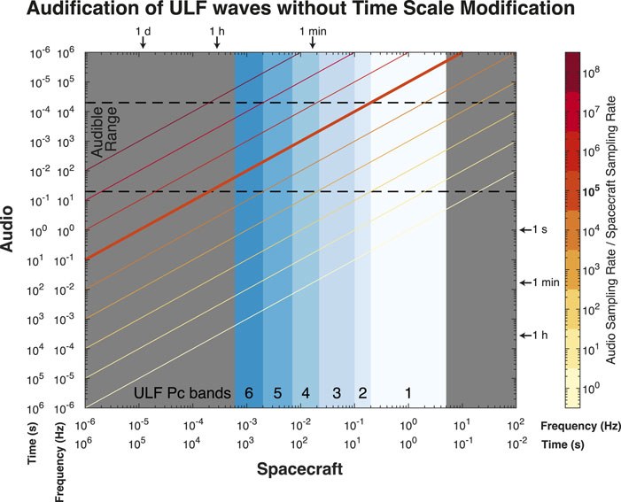
FIGURE 1. Relationship between spacecraft time and frequency to audio time and frequency in audification for different ratios of sampling rates. ULF wave bands are also highlighted.

Alexander et al. (2011, 2014) and Wicks et al. (2016) showed that researchers using audification applied to Wind magnetometer data in the solar wind aided in the identification of subtle features present that were not necessarily clear from standard visual analysis. Archer et al. (2018) similarly showed that audification of GOES magnetic field observations enabled high school students to identify numerous long-lasting decreasing-frequency poloidal field line resonances during the recovery phase of geomagnetic storms. Such events were previously thought to be rare, but through exploration of the audio they were in fact demonstrated to be relatively common. These preliminary studies into the use of audification of the ULF wave bands within heliophysics show promise in its potential scientific applications.

Direct audification may not, however, be suitable for all space plasma missions and/or ULF wave events. Figure 1 indicates that to make the ULF bands audible necessarily renders a day of data into about one second of audio. In geostationary orbit the background plasma and magnetic field conditions, which affect the eigenfrequencies of the ULF modes, are relatively stable across the orbit (Takahashi et al., 2010). This makes identifying the local time patterns in frequency and occurrence of ULF waves relatively straightforward (Archer et al., 2018). However, for more eccentric orbits with similar orbital periods the conditions, frequencies, and occurrence of ULF waves will rapidly change throughout the orbit (Archer et al., 2015, 2017). Therefore, the rate at which ULF waves’ properties may be changing in the audio will be very fast. This is demonstrated in the audio in Supplementary Data S1 of Archer et al. (2022), where audification is applied to idealised and real events from the THEMIS mission. It is clear from this audio that changes are occurring too quickly to effectively listen to and analyse. Another potential issue in audification is that ULF waves can be highly transient, occuring for only several oscillations due to intermittent driving and/or damping (e.g. Zong et al., 2009; Wang et al., 2015; Archer et al., 2019). This means that ULF wave events which persist for only $\sim 10\text{–}30\mathrm{m}\mathrm{i}\mathrm{n}$ will last only $\sim 60\text{–}200\mathrm{m}\mathrm{s}$ in the audio. Furthermore, effective pitch discrimination by the auditory system often requires several tens of (and even up to a hundred) oscillations (Fyk, 1987), which is not always the case with ULF waves. Thus, improvements to the sonification process over simple audification are clearly required for application to magnetospheric ULF waves more widely.

In this transdisciplinary paper we introduce several potential improved sonification methods for ULF waves, borrowing techniques from the fields of audio and music. The properties of the resulting audio from these different methods are assessed through a public dialogue with stakeholder groups to arrive at recommendations for ULF wave researchers on how best to render these waves audible. Finally, we discuss the scientific and educational possibilities that might be enabled by these new methods.

2 Sonification

Taking existing techniques from the fields of audio and music, we have developed new potential sonification methods for magnetospheric ULF waves which we detail throughout this section. In this work we focus on Alfvén waves (Southwood, 1974), arguably the most intensely studied mode of ULF waves (e.g. the review of Keiling et al., 2016). Further justifying this choice is the fact that significant coupling occurs within the magnetosphere from compressional to Alfvén modes due to plasma inhomogeneity, curvilinear magnetic geometry, and hot plasma effects (Southwood and Kivelson, 1984). However, this focus does not preclude that sonification might also render other types of ULF waves that also occupy the same Pc3–6 frequency bands, such as surface (e.g. Archer et al., 2019) or waveguide (e.g. Hartinger et al., 2013) modes, effectively audible, though these applications are beyond the scope of this paper. The natural frequencies of Alfvén waves vary with local time and L-shell, with the spectrum of frequencies with location being known as the Alfvén continuum. The typically reported trend is that, outside of the plasmasphere or plumes, Alfvén wave frequencies tend to decrease with radial distance from the Earth (Takahashi et al., 2015), hence spacecraft observations often show tones whose frequencies sweep from high to low as the probe follows its orbit from perigee to apogee (and vice versa as the orbit continues from apogee back to perigee). It is worth noting though that the Alfvén continuum can vary considerably, both in terms of absolute values and morphology, with solar wind and magnetospheric driving conditions (Archer et al., 2015, 2017).

The full sonification process developed here is outlined as a flow chart in Figure 2. Throughout we apply the methods to NASA THEMIS observations (Angelopoulos, 2008), chosen due to the highly eccentric equatorial orbits of its spacecraft with the inner three probes having apogees r ∼ 12–15 R_E and perigee r ∼ 1.5 R_E over the course of the mission. Spin-resolution data is used, with one data point every 3 s (any data gaps or irregular samples are regularised by interpolation). As with Archer et al. (2018) we focus only on waves in the magnetic field, using fluxgate magnetometer data (Auster et al., 2008; electron plasma data, McFadden et al., 2008, is also used for discriminating between magnetosphere and magnetosheath intervals). Other physical quantities such as the plasma velocity (e.g. Takahashi et al., 2015) or electric field (e.g. Hartinger et al., 2013) could also be used in the sonification of ULF waves—a prospect we leave to future work. How the different potential sonification methods affect the sound of the resulting audio is assessed in Section 3. The software developed incorporating all of these methods is available at https://github.com/Shirling-VT/HARP_sonification.

FIGURE 2

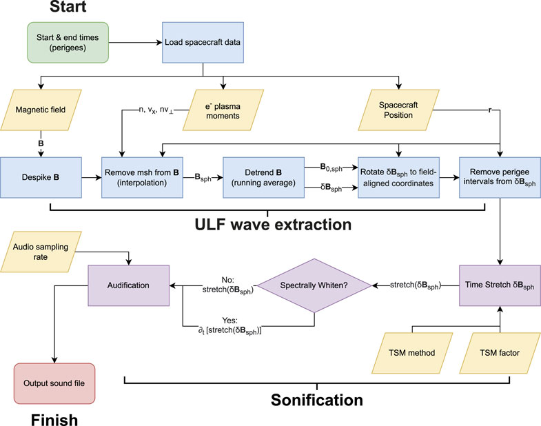
FIGURE 2. Flow chart of the sonification processes used.

2.1 ULF Wave Extraction

Before sonification, the magnetospheric ULF waves must be extracted from the data and transformed into an appropriate coordinate system. Non-physical spikes in the magnetometer data are first removed by identifying when ∂_tB > 3 nT s⁻¹ in any component and removing the 10 neighbour data points from all components. Next, since magnetospheric ULF waves are the focus of the sonification, magnetosheath intervals are also removed. These are flagged for r > 8 R_E when either the electron number density is greater than 10 cm⁻³, antisunward component of the electron velocity is greater than 200 km s⁻¹, or the perpendicular electron particle flux is greater than 2 × 10⁷ cm⁻² s⁻¹. The three nearest neighbour points to flagged data are also removed. Interpolation is applied to fill in the removed data, thereby preventing discontinuities in the data which might affect the sonification. For short magnetosheath intervals, less than the dominant ULF wave period present, the interpolation will fill in the gaps in phase effectively. In contrast, when the intervals are longer than ULF wave periodicities then the resulting audio during interpolated intervals will be silent, since frequencies associated with the interpolation will be below the audible range.

The background magnetospheric magnetic field is determined by a 30 min running average, with this trend being subtracted to arrive at the ULF waves. These are then rotated into a field-aligned coordinate system. The field-aligned component (representative of compressional waves) is along the previous running average, the radial component (representative of poloidal waves) is perpendicular to this pointing radially away from Earth, and the azimuthal component (representative of toroidal waves) is perpendicular to both of these pointing eastwards. Since close to Earth the instrument precision is reduced (Auster et al., 2008) and the dipole field as measured by the spacecraft changes more rapidly than the running average (Archer et al., 2013), we finally remove all data from geocentric distances r < 5 R_E setting these points to zero.

2.2 Time Scale Modification

Time scale modification (TSM) refers to speeding up or slowing down audio without affecting the frequency content, e.g. the pitch of any tones (Driedger and Müller, 2016). It therefore modifies the link between the time of events and frequency/periodicity of waves. This may be advantageous for the sonification of ULF waves compared to simple audification, since it allows the frequencies to still fall within the audible range as per Equation 2 but stretches the audio in time so that events do not occur so quickly for listening, i.e.

$\mathrm{\Delta }\left(\mathrm{A}\mathrm{u}\mathrm{d}\mathrm{i}\mathrm{o}\mathrm{t}\mathrm{i}\mathrm{m}\mathrm{e}\right)=\mathrm{T}\mathrm{S}\mathrm{M}\mathrm{f}\mathrm{a}\mathrm{c}\mathrm{t}\mathrm{o}\mathrm{r}\times \mathrm{\Delta }\left(\mathrm{S}\mathrm{p}\mathrm{a}\mathrm{c}\mathrm{e}\mathrm{c}\mathrm{r}\mathrm{a}\mathrm{f}\mathrm{t}\mathrm{t}\mathrm{i}\mathrm{m}\mathrm{e}\right)\times \frac{\mathrm{S}\mathrm{p}\mathrm{a}\mathrm{c}\mathrm{e}\mathrm{c}\mathrm{r}\mathrm{a}\mathrm{f}\mathrm{t}\mathrm{s}\mathrm{a}\mathrm{m}\mathrm{p}\mathrm{l}\mathrm{i}\mathrm{n}\mathrm{g}\mathrm{r}\mathrm{a}\mathrm{t}\mathrm{e}}{\mathrm{A}\mathrm{u}\mathrm{d}\mathrm{i}\mathrm{o}\mathrm{s}\mathrm{a}\mathrm{m}\mathrm{p}\mathrm{l}\mathrm{i}\mathrm{n}\mathrm{g}\mathrm{r}\mathrm{a}\mathrm{t}\mathrm{e}}(3)$

Here the TSM factor refers to the factor by which the audio has been stretched in time, where values greater than one result in longer audio (in some other sources the definition may refer to the reciprocal of this). Time stretching necessarily increases the number of oscillations present in each event, since the periodicities are maintained and thus Equation 2 remains unaffected. This has the consequence of also improving the audibility of short-lived waves for purposes such as pitch detection (Fyk, 1987).

One of the benefits of direct audification is that the resulting audio is identical in information content to the original data. While TSM methods necessarily modify their inputs, this is done in ways which are relatively easy to understand. In principle, it should be possible to reverse these procedures to arrive back at the original data, which we justify for each method in turn. However, in practice some additional artifacts may be present when attempting this reversal. Nonetheless, key properties of the original data are left invariant by each process and thus the time-stretched audio can still be treated as a representation of the original data. Because different TSM methods work differently though, it is expected that the methods will produce audio that sounds different.

In this subsection we briefly describe several widely used TSM methods, originally developed primarily for music, which we will apply to ULF wave observations. For further discussion of the details behind these methods see the review of Driedger and Müller (2016) and/or our provided software. Throughout this subsection the input refers to the extracted ULF waves from the original spacecraft time series, consisting of N data samples (the spacecraft time range used multiplied by the spacecraft sampling rate). Several of the methods are based on overlap–add procedures. These take analysis frames, highly overlapping windows spaced by the analysis hop, from the input data. Throughout we have set the length of the analysis frames to be 512 samples (25 min) as this is the closest power of two to the length of the running average used to extract the waves. The analysis frames are individually manipulated, depending on the TSM method used, and then relocated on the audio time axis as synthesis frames with corresponding synthesis hop. The slightly overlapping synthesis frames are then added together, essentially performing multiple copies of very similar parts of the original data, yielding the output. This gives the desired TSM of the input data by a stretch factor equal to the ratio of analysis to synthesis hops. The output thus contains more data samples but covers the same spacecraft time range in UTC, with the periodicities of oscillations (shorter than the frame length) in terms of data samples having been preserved. In general one has a freedom in what fraction of the frame length to use as the synthesis hop. This has been tested and we report which choices seemed to yield the best results when applied to magnetospheric ULF waves. Mathematically it is possible to reproduce the original signal following an overlap-add procedure with no modifications subject to some simple constraints on the windowing function (Sharpe, 2020). Therefore, if the modifications are also invertible then overlap-add based TSM methods should also be reversible. Supplementary Figure S1 shows an example of applying first stretching and then compression of time for each TSM method to an idealised chirp ULF wave signal with added noise.

2.2.1 Waveform Similarity Overlap-Add

Waveform Similarity Overlap-Add (WSOLA) is a TSM method that works in the time domain as outlined in Figure 3. The only modification between the analysis and synthesis frames are slight shifts in time to reduce any phase jumps present in the output, with these shifts being determined for each successive frame via cross correlation (Driedger and Müller, 2016). As a time-based procedure WSOLA is known to have issues with transients much shorter than the analysis frame length, causing these features to be repeated in the output. WSOLA is also known to struggle when multiple harmonic sources are present, with only the largest amplitude one being preserved in the output. For continuous functions with no noise, the cross-correlation function should be smooth with a well-defined peak. Therefore, the time-shifts applied in WSOLA are invertible in principle. However, in practice the discrete-time nature of digital data and the presence of substantial noise may hinder the invertibility of WSOLA. The WSOLA example in Supplementary Figure S1 (blue) shows that the original periodicities are recoverable, but amplitudes and longer-term trends may end up being rather different.

FIGURE 3

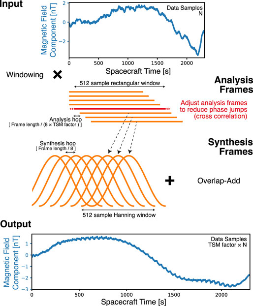
FIGURE 3. Illustration of the Waveform Similarity and Overlap Add (WSOLA) method.

2.2.2 Phase Vocoder

The phase vocoder TSM is a frequency domain overlap–add procedure that aims to preserve the periodicities of all signal components. Figure 4 depicts how it works through a Short Time Fourier Transform (STFT). Due to the coarse nature of this transform in both time and frequency, to maintain continuity in the output the STFT phases at each frequency need to be iteratively adjusted (based on the phase differences between frames) before inversion, known as phase propagation (Driedger and Müller, 2016). Therefore, the STFT spectrogram (absolute magnitude of the transform) remains invariant under the phase vocoder (note human hearing is relatively insensitive to phase; Meddia and Hewitt, 1991; Moore, 2002). Transient signals tend to get somewhat smeared out over timescales of around the frame length using this method. While locking the phase of frequencies near peaks in the spectrum can reduce phase artifacts, these nonetheless may still be present and are reported to have rather distinct sounding distortions. The STFT is known to have an inverse transform, however, again in practice the discrete application of this transform to noisy data can result in artifacts such as time-aliasing (Allen, 1977). The example of its invertibility in Supplementary Figure S1 (orange) demonstrates it performs slightly better than WSOLA at recovering the original data.

FIGURE 4

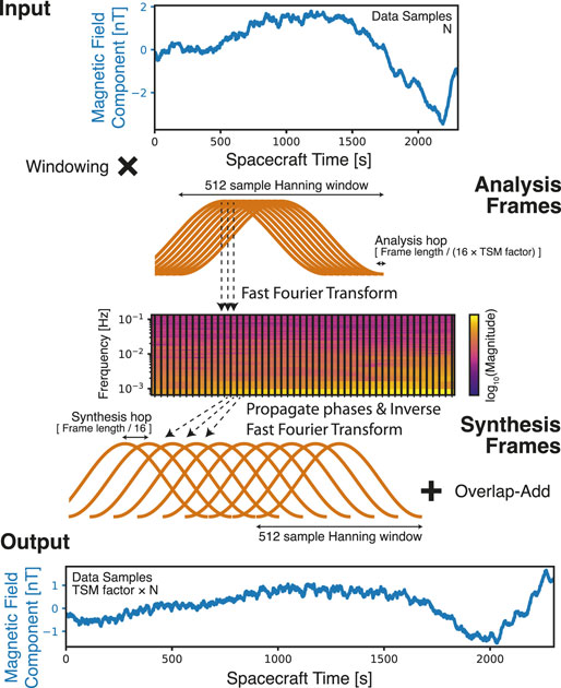
FIGURE 4. Illustration of the Phase Vocoder method.

2.2.3 PaulStretch

PaulStretch is an extreme sound stretching algorithm based on the phase vocoder (Nasca, 2006). Instead of propagating the phase, which becomes difficult for large TSM factors, the algorithm instead randomises all the STFT phases, as shown in Figure 5. This results in a more smooth sound than the phase vocoder method, with less repetition and distortion (Nasca, 2010). Unlike the other methods presented here, PaulStretch is not suitable for TSM factors less than unity (compression in time) as it will result in many phase jumps due to the randomisation. The method may also result in the introduction or modulation of amplitudes over timescales of the order of, or longer than, the frame length, which while visible in the waveforms are not noticeably audible typically. Since random numbers are applied to the phase, this method would only be invertible if those random numbers were saved as part of the process. Nonetheless, like the phase vocoder, PaulStretch leaves the STFT spectrogram invariant.

FIGURE 5

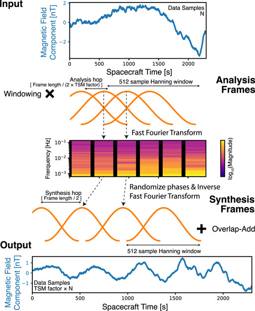
FIGURE 5. Illustration of the PaulStretch method.

2.2.4 Wavelet Phase Vocoder

The wavelet phase vocoder technique (henceforth simply wavelets) works rather differently to the previous overlap-add procedures, as illustrated in Figure 6. It utilises a complex continuous wavelet transform of the data (Torrence and Compo, 1998), a complete time-frequency (over) representation of the data which consistently scales these two dimensions with one another (unlike the STFT). This has the benefit that magnitude and phase are provided at each frequency for all sampling times, rather than only at a small number of specified analysis frames. The TSM procedure is simply an interpolation in time of the wavelet coefficients (essentially different bandpasses) followed by multiplying the unwrapped phase by the TSM factor (De Gersem et al., 1997). The interpolation step increases the number of samples, lowering the pitch of oscillations, which is subsequently corrected by rescaling the phases by the same factor. The modified wavelet coefficients are then inverted back to a time-series (Torrence and Compo, 1998). While wavelet reconstruction is possible mathematically for continuous functions, it has been noted that this is often not perfect in practice computationally (Lebedeva and Postnikov, 2014; Postnikov et al., 2016). The example of inversion in Supplementary Figure S1 (yellow) shows a constant phase offset has resulted, likely due to edge effects, but otherwise the wavelet phase vocoder performs somewat similarly to its STFT counterpart. The wavelet spectrogram is invariant under this TSM method.

FIGURE 6

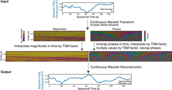
FIGURE 6. Illustration of the Wavelet phase vocoder method. Note the shorter time range presented due to the different method.

2.3 Spectral Whitening

The amplitudes of ULF wave magnetic field oscillations in general are largest at the lowest frequencies and tend to decrease rapidly with increasing frequency. This pattern is associated mostly with incoherent background noise, whose overall levels vary depending on driving and magnetospheric conditions, on top of which discrete resonances may also be present. However, because of this trend, spectrograms tend to show undue prominence to the lowest frequencies, making variations present at higher frequencies hard to discern. Therefore, it is common to pre-whiten ULF wave spectra so that the background spectrum is flat. A simple way to achieve this is through taking the time derivative of the time-series before calculating spectra, since the amplitudes approximately follow a 1/f Brownian/red noise relationship (e.g. Engebretson et al., 1986; Russell et al., 1999). Such spectral whitening may also be helpful for similar reasons in the sonification of ULF waves. Indeed, Archer et al. (2018) produced audifications of both the original and time-derivatives of the data. Here the whitening step is optionally undertaken after TSM, since it was found that applying it beforehand had adverse effects on the time stretching.

2.4 Audification

The final step is audification. To ensure that the audio waveforms are constrained to the dimensionless range −1 to +1, the data is normalised by the maximum absolute value. This normalised data is then written to audio using a standard audio sampling frequency of 44,100 Hz, which as discussed earlier renders most of the ULF wave bands audible since THEMIS measurements are made every 3 s (Figure 1). While Archer et al. (2018) produced separate mono tracks for each component of the magnetic field and a combined stereo file containing all three components, here we only produce the separate files, focusing in particular on the azimuthal component of the magnetic field as this is most relevant to the Alfvén continuum (Southwood, 1974). The audio is encoded in Waveform Audio File Format (WAV), an uncompressed and the most common audio format. Archer et al. (2018) had used Ogg Vorbis compression, which is near-lossless thereby reducing the file size efficiently, however, we found that not all applications were able to robustly work with this format (issues with the MP3 format introducing silence to the audio eliminating the ability to relate audio time to spacecraft time were highlighted by Archer et al., 2018).

3 Public Dialogue

It was felt that in order to provide recommendations to ULF wave researchers on the best method of rendering these waves audible that we should seek input from various stakeholder communities outside of the space sciences. This is because these communities either have expertise in audio and its usage, or form intended target audiences for the sonified ULF waves. We therefore undertook a public dialogue on the different sonification methods presented. The study gained ethical approval through Imperial College London’s Science Engineering Technology Research Ethics Committee process (reference 21IC7145).

3.1 Methods

An anonymous online survey was used for the public dialogue, where participants were asked to rank audio clips and explain their reasoning. Survey questions can be found in Supplementary Table S1. The audio clips in each question varied either the TSM method, TSM factor, or background noise spectrum. These were applied to three different THEMIS events. It was deemed that having more than three events would limit participation, due to the amount of time it would take to complete the survey, and that the events chosen provided a good range in ULF waves to apply the different methods to. Each event corresponds to 3 full orbits of the THEMIS-E spacecraft starting and ending at perigees, and thus are approximately 3 days in duration. They are shown in Figure 7. Event 1 corresponds to a synthetic Alfvén continuum—a constant amplitude chirp/sweep signal, i.e. $\sin \left(\mathrm{\Psi }\left[t\right]\right)$ with instantaneous frequency $f\left[t\right]={\partial }_t\mathrm{\Psi }\left[t\right]/2\pi$. The frequencies are taken from the statistical Alfvén continuum calculations of Archer et al. (2015, 2017) based on a large database of THEMIS density observations. The average frequencies in the dawn sector as a function of L-shell (neglecting plasmaspheric densities and assuming local azimuthal symmetry) have been constructed and then mapped to a representative orbit. The first orbit consists of the fundamental frequency plus low-level (standard deviation of 10% the chirp amplitude) Brownian noise (Gardiner, 2009); the second orbit is a superposition of the first and third harmonics (each at half the previous amplitude) plus more intense noise (3 times greater); and the third orbit is just the high-level of noise. The other two events correspond to real data under different conditions. Event 2 covers 17–20 March 2012, where THEMIS was in the dawn sector (05:40 MLT at apogee) and geomagnetic conditions were active (minimum Dst was −44 nT). Event 3 covers 21–24 July 2011, where THEMIS was in the dusk sector (19:55 MLT at apogee) and geomagnetic conditions were moderate (minimum Dst was −20 nT). All the audio clips used in the survey can be found in Supplementary Data 2 of Archer et al. (2022) or in the survey preview link provided.

FIGURE 7

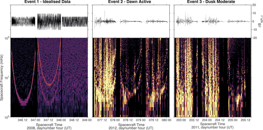
FIGURE 7. The three example THEMIS ULF wave events used in the survey. Top panels show the azimuthal component of the magnetic field with bottom panels showing its Short Time Fourier Transform spectrograms with a logarithmic colour scale, where the background has been spectrally whitened.

3.1.1 Participants

Participants were recruited by advertising the study to public email lists for those with relevant interests/expertise, such as music, citizen science, or science communication. Social media posts were also used. A total of 140 people completed the survey over the month it was open, all of whom indicated their consent as part of the survey itself. A breakdown of participants’ self-identified expertise, shown in Supplementary Figure S2, reveals we successfully targeted the survey outside of the space science community, with a good mix of interest groups.

3.1.2 Analysis

Both quantitative and qualitative analyses are employed, as the closed and open questions in the survey generate different types of data.

The quantitative data comes in the form of rankings, where a rank of 1 corresponds to the most liked/favoured (i.e. the highest ranked) and r_max corresponds to the least liked/favoured (i.e. the lowest ranked). The proportions of all responses p_i in each rank r_i is determined. Based on these, for each audio clip we construct a score calculated as

$\mathrm{S}\mathrm{c}\mathrm{o}\mathrm{r}\mathrm{e}=\sum _{i=1}^{r_{\mathit{max}}}\frac{r_{\mathit{max}}-2r_i+1}{r_{\mathit{max}}-1}{p}_i(4)$

where the fraction normalises each rank value to between −1 (least liked) and +1 (most liked), hence the score is also constrained to this range. The scores are then averaged over the three events to give an overall score for that option. 95% confidence intervals in these overall scores are estimated by bootstrapping the same calculations over the participants (Efron and Tibshirani, 1993), where 5,000 different random samples with replacement are employed.

Thematic analysis (Braun and Clarke, 2006) is used to analyse the meaning behind the open-text questions. This finds patterns, known as qualitative codes, in the data which are then grouped into broader related themes. The themes and codes are defined by induction, where they are iteratively determined by going through samples of the qualitative data rather than being pre-defined (Silverman, 2010; Robson, 2011). Once finalised, the themes and codes are applied to the full dataset by the primary coder and indicative quotes are identified. A second coder independently analysed a subset of the data (30 participants’ responses, corresponding to 21%) to check reliability. Average agreement across the different themes ranged from 73 to 95%. A typical measure of reliability in coding qualitative data is Cohen’s kappa, a statistic between 0 and 1, given by unity minus the ratio of observed disagreement to that expected by chance (McHugh, 2012). Average values between 0.5 and 0.6 were found across the themes, which correspond to 70–80% of the maximum achievable values given the uneven distributions of the data (Umesh et al., 1989). All these statistics therefore indicate good agreement and thus the qualitative analysis is reliable.

3.2 Results

All participants’ responses to the survey question can be found in Supplementary Data S3. The quantitative results of the survey are shown in Figure 8, depicting the proportions in each rank for the various options as well as their scores. No obvious trends were present in the quantitative results between different interest groups, hence we simply present all the data together in this paper. Table 1 summarises the themes and their underlying codes that were determined from the qualitative data, as well as which question topics these pertained to. The application of these qualitative codes to the open responses can be seen in Supplementary Data S4 of Archer et al. (2022). One of the main themes was timbre, which refers to the perceived quality of a sound. This theme encapsulates aspects of whether the sounds were pleasant to listen to or if potential issues around ear fatigue were raised. The codes in this theme thus are either positive, negative, or neutral. The second theme concerned signal-to-noise or the perceived information content within the sounds, i.e. whether the tones were discernible from the background. Again the codes ranged from positive, through to neutral, or negative. Issues around potential artifacts introduced by the processing were raised as another theme. Many respondents also commented with synonymous sounds, i.e. what they thought the audio “sounded like”. The final themes/codes concerned whether it was possible to hear the detail present, if listening to the sounds evoked a sense of boredom, and if the participants desired more context on the intended usage of the sounds. All these themes were present across the different interest groups. Not every participant answered all the open-text questions, with response rates between 88 and 94%. Some answers did not fit into all of the themes either, with the two main themes of timbre and signal-to-noise being discussed on average in 41% and 30% of responses respectively.

FIGURE 8

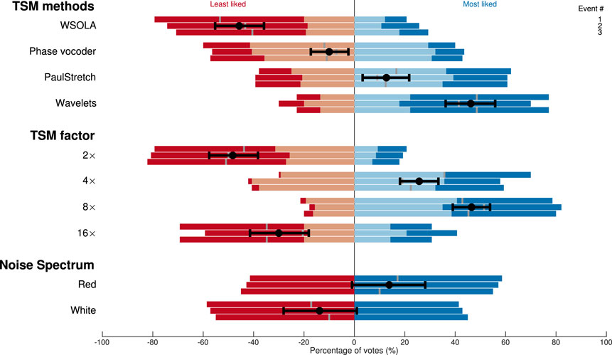
FIGURE 8. Quantitative results of the survey. Stacked bars show the proportions of each ranking from least liked (dark red, far left) to most liked (dark blue, far right). The score for each audio clip is indicated by the grey bars, with the overall score across all 3 clips for each group shown as the black marker along with its 95% confidence interval. Note that for TSM methods and TSM factors there were four possible options, and thus also four possible ranks, while for noise spectrum there were only two.

TABLE 1

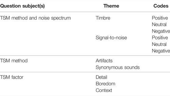
TABLE 1. Themes and codes from the qualitative data.

3.2.1 TSM Methods

Figure 8 indicates that the wavelets technique was by far the participants’ favourite TSM method. Its timbre was deemed to be the most pleasant to the ear, with 57 positive responses compared to only 5 neutral and 3 negative

“The best on all counts. Good depth, and richness in texture.” (Participant 3)

“This had a softer sound, easier to listen to.” (Participant 41)

Many participants (a total of 37) noted that the results of this method evoked the sounds of water. In terms of the signal-to-noise, 26 responses indicated that the tones were sufficiently clear

“Conveyed the frequencies effectively.” (Participant 6)

“Clearly isolates the components of the signals.” (Participant 56)

Only 7 expressed the wavelets method was too noisy, though 16 responses indicated more neutral responses within this theme

“Very ‘harmonic’ sounds, but occasionally hard to differentiate.” (Participant 45)

PaulStretch had the second highest overall score. Generally it’s timbre was thought of as positive (32 responses) but more neutral (14) and negative (13) comments were made than with wavelets

“I like it, makes sounds very smooth and kind of diffuse.” (Participant 15)

“This was also pleasing, but a little less than Wavelets.” (Participant 84)

“Kind of a middle ground between the watery feel of Wavelets and the glitchy techno of the other two” (Participant 14)

“Felt very static filled and hard to listen to.” (Participant 128)

The most common synonymous sounds were those of wind or “natural” sounds. The survey results were inconclusive on the signal-to-noise ratio present with PaulStretch.

The phase vocoder method was ranked only slightly below PaulStretch—several participants noted similarities in the sounds of the two, which is due to their related methods. However, open responses were more negative (36 responses) on how this method sounded

“Sounds like really terrible radio interference and is very jarring to the nerves.” (Participant 35)

“The metallic character made it less pleasant to listen to” (Participant 25)

Compared to 17 neutral and 6 positive comments. Results were again mixed on the information content, however, potential artifacts associated with this method were more commonly raised than before (12 responses)

“This sounds like heavily processed noise cancelling DSP (digital signal processing) which maybe good at recovering spoken words but heavily masks fundamental random signals.” (Participant 55)

“Most unpleasant; phasing is the culprit.” (Participant 88)

WSOLA was clearly the least liked TSM method in the rankings. Indeed, almost all comments on the sound quality were negative (70 responses)

“Too much distortion for my taste, hard for me to listen to.” (Participant 86)

“Totally unlistenable. It sounds like 4-bit digital audio.” (Participant 129)

“Lack of amplitude dynamic[s] makes it almost painful to listen.” (Participant 135)

Similar to with the phase vocoder, results on the signal-to-noise were inconclusive and processing artifacts were raised several times (17 responses)

“Distortion artifacts are probably not real” (Participant 56)

“Too much artificial noise sounds.” (Participant 103)

Therefore, the recommendation from our survey is that the wavelet phase vocoder method is the preferred TSM method for application to magnetospheric ULF waves. It may be possible to improve this method even further by compensating for the spreading effects in time-frequency due to the mother wavelet. Examples of this are the synchrosqueezed wavelet transform (Daubechies et al., 2011) which uses reassignment in frequency, or superlets (Moca et al., 2021) which is a geometric combination of sets of wavelets with different bandwidths. Further work into how one may apply these to TSM is required.

3.2.2 TSM Factor

The result of the rankings shown in Figure 8 shows that a TSM factor of 8× was favoured, with 4× somewhat close behind (this difference is statistically significant though). TSM factors of 2× and 16× were both ranked poorly and the confidence intervals in their overall scores overlap. The reason behind these scores could be gleaned from the open-text responses. Participants stated that larger TSM factors allowed more time to hear the detail of the signals within the clips, which was not possible with the shortest clips (44 responses)

“Length of audio clips coincided with perception of individual tones and increased clarity of sounds as the length increased.” (Participant 5)

“I much prefer the longer audio lengths, because it allows me to hear the nuances in the received sound.” (Participant 78)

“The 2x signal goes by too fast. Listener will miss small changes in the signal.” (Participant 59)

However, in contrast, it was felt that the longest clips may induce boredom in the listener (30 responses)

“While having a 30 second clip would be ideal, it feels tedious and boring and not ‘fun’ to listen to. It also can be quite painful to listen to some of the tracks at full length.” (Participant 5)

“Generally the 16× feels dragging too slow and information can be obtained from faster speeds.” (Participant 20)

Thus the consensus was that the two middle options provided a compromise to both these themes, though individuals’ preferences varied between 4× and 8×. 11 participants raised that to best answer the question on the TSM factor they would have preferred to know more about the context of the sounds, their intended uses, and any tasks associated with them. We intentionally did not provide this, however, as our aim was to arrive at broad recommendations on the sonification of magnetospheric ULF waves that may be applied in a variety of contexts and settings.

The recommendation on TSM factor from the survey would be to use a value of $\sim 6\times$, based on the average (either arithmetic or geometric) TSM factors for 4× and 8× using the overall scores as weights.

3.2.3 Noise Spectrum

Participants’ preferences in terms of the background noise spectrum of the audio were somewhat split, as shown in Figure 8, with overall 57% preferring red noise (audification of B) to white noise (∂_tB). The confidence intervals for the scores also are not constrained to simply positive or negative. Therefore, the quantitative results do not provide a clear recommendation. However, the qualitative data provides further insight. While opinions on which had the more pleasant timbre were again somewhat split, comments on the harshness of the white noise (23 responses) outweighed those of the red (8 responses) with many references to the higher frequencies present being the cause of this

“The white noise has higher frequencies, which is giving me some ear fatigue.” (Participant 19)

“This noise hurts my ears and gives me a headache. It is sharper and tinnier.” (Participant 26)

However, it was recognised that the spectral whitening made it easier to distinguish the signals (30 responses) whereas the red noise sounded somewhat “muffled” and less clear.

“The tones seemed clearer against this as a backdrop.” (Participant 21)

“This process provides a full spectrum appreciation of the underlying signals that are not bandwidth limited due to masking or filtering.” (Participant 55)

The spectral whitening of ULF waves is used to make signals over a wide range of frequencies clearer in spectrograms, since the background spectrum becomes approximately constant with frequency (Engebretson et al., 1986; Russell et al., 1999). The same power value in the spectrogram relative to the background at different frequencies therefore can be seen as the same colour on the chosen colourmap. However, the survey results highlight that the same level of intensity of sound at different frequencies are not perceived as the same loudness. Indeed, human hearing is most sensitive to higher frequencies in the range 2–5 kHz, which is likely the reason for the comments on the harshness of the white noise. Equal-loudness contours have been determined, which specify what sound pressure levels at different frequencies are perceived as being at the same loudness level (International Organization for Standardization, 1987; Suzuki, 2004). Therefore, rather than modifying the spectrum of the ULF waves for sonification to be flat in intensity they should be adjusted for equal-loudness, which should be possible through applying appropriate filtering (e.g. by modifying the magnitudes of the Fourier transform after stretching). This should then have the benefits of making tones discernible but not being too harsh on the ears.

4 Discussion

While time-series data of magnetospheric ultra-low frequency (ULF) waves are often still analysed visually (at least in part), this form of data lends itself more naturally to our sense of sound. Direct audification is the simplest sonification method, providing a true representation of the original data. When applied to ULF waves though this can result in changes occurring too rapidly for effective analysis by the human auditory system. Therefore, we detail several existing audio time scale modification (TSM) techniques which have been applied to ULF wave data. Through a public dialogue with stakeholder groups, we arrive at recommendations on which sonification methods should be used to best render the Alfvén waves present audible, which are summarised in Table 2. We have implemented these final recommendations, applying them to the three THEMIS example events yielding the audio in Supplementary Data S5 of Archer et al. (2022).

TABLE 2

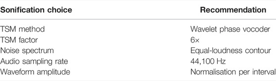
TABLE 2. Final recommendations on ULF wave sonification.

Figure 7 shows a typical spectrogram representation of ULF waves for the three examples, where the logarithmic colour scale has been spectrally whitened and the limits of the colour scale in each individual event have been set at the 50% (corresponding to the noise level) and 95% (corresponding to the peaks) percentiles in power in order to capture the range present. In the idealised data (event 1) the Alfvén continuum, with frequencies decreasing from perigee to apogee, is very clear. In contrast, in the real data (events 2–3) identifying discrete peaks even by visual inspection is much more difficult. Even in the dawn sector under active geomagnetic conditions, where standing toroidal Alfvén waves are more common and their frequency profiles should be simpler (i.e. similar to event 1; Takahashi et al., 2016; Archer et al., 2017), the continuum is still subtle, especially for the first orbit where significant incoherent broadband wave power is also clearly present. In contrast, the Alfvén continuum is clearly audible in Supplementary Data S5 (Archer et al., 2022) throughout portions of the orbits for all three events. The auditory system’s ability to identify these subtle sweeping frequency tones in the presence of significant noise and other potential signals is likely thanks to its nonlinear nature and impressive ability at blind source separation. It is well known that all wave analysis techniques have their advantages and drawbacks, which will depend on the nature of the precise oscillations present (Chi and Russell, 2008; Piersanti et al., 2018). Sonification can thus provide an additional supportive tool for researchers in identifying different ULF waves (Alexander et al., 2011, 2014; Wicks et al., 2016; Archer et al., 2018) that may complement other techniques. By maximising the audibility of ULF waves for more challenging orbits/environments/events, the methods presented here should hopefully improve further the utility of sonification in this science topic.

Another benefit to sonification is that it renders scientific data more accessible and lowers the barrier to entry for students and the public to contribute to space science through citizen science (Archer et al., 2018). With the growing number of space plasma spacecraft in orbit around Earth and the networks of ground magnetometers globally, we are continually producing big data that poses a challenge to efficiently navigate, mine, and analyse. Machine learning is typically the emerging solution to dealing with big data in general, with supervised machine learning techniques being applied to a variety of space physics tasks (e.g. Breuillard et al., 2020; Lenouvel et al., 2021). However, current challenges in ULF wave research mean that many simple tasks (e.g. classifying ULF wave events) are still not easily tackled by these methods due to the lack of good (e.g. classified) training sets of events. Until ULF wave research can be fully automated, clearly it is not feasible for a single researcher to visually inspect all the ULF wave data that is, being produced. The dramatically reduced analysis processing time associated with listening to sonified data (even with moderate TSM applied) certainly helps. However, any manual process applied by a single researcher is potentially subject to biases and concerns over reliability. On the other hand, mobilising citizen scientists en masse to cover these vast datasets and arrive at a statistical consensus for each interval/event may in fact be more robust (e.g. Barnard et al., 2014). Therefore, there is a lot of potential in applying the sonification methods presented here to arrive at new scientific results through citizen science. A simple example is that already discussed, identifying how the properties and excitation of the Alfvén continuum vary under different solar wind and geomagnetic driving conditions—an important and still unresolved issue (e.g. Rae et al., 2019). Another possibility is that citizen scientists collectively may be able to arrive at more data-driven classifications of ULF waves that take into account further properties of the waves than simply frequency, which may better distinguish between the different physical processes at play than the current scheme (Jacobs et al., 1964). Countless other scientific questions into the sources and propagation of ULF waves in planetary magnetospheres could be addressed through citizen science with sonified data. Indeed the pilot “Heliophysics Audified: Resonances in Plasmas” (HARP) citizen science project (http://listen.spacescience.org/) is already building on the work presented by Archer et al. (2018) in this area, developing more streamlined interfaces for citizen scientists to interact with the audible data and record scientific results. A result of increased citizen science in ULF wave research could be the very training sets required to be able to apply machine learning algorithms to the data, an approach which has successfully been done in other fields (e.g. Beaumont et al., 2014; Sullivan et al., 2014). Once trained, these machine learning algorithms would then be able to tie together multi-satellite and multi-station data of the same event at different locations, in ways which are not possible with a single audio stream, to improve our global understanding of system-scale magnetospheric dynamics under different driving regimes.

More work is required to understand the full scope of sonification in the identification, categorisation, and characterisation of the zoo of ULF waves present within Earth’s magnetosphere. The application of existing TSM methods from the field of music and audio in this paper was motivated by the short timescales associated with direct audification of ULF waves and limits in human’s pitch perception based on the number of oscillations in typical ULF wave events. While this work has certainly increased the audibility of ULF waves, the Alfvén continuum in particular, only through further work in applying sonification for the purposes of novel scientific results can the full benefits and limits of these tools be realised.

Beyond potential scientific benefits, there are also obvious uses of sonified ULF waves in education, engagement, and communication. Recently a number of high-profile ULF wave results have leveraged the methods presented in this paper within press releases for the media (National Centers for Environmental Information, 2018; European Space Agency, 2019; Johnson-Groh, 2019; Tran, 2021), which have gone on to successfully attract global attention. Therefore, sonification is a helpful tool in communicating our science. Archer et al. (2021a) showed that simply enabling public audiences to experience these sounds can spark innate associations and dispell common misconceptions simply through the act of listening, highlighting the power of the medium in its own right. This has similarly been reflected in many of the survey responses of synonymous sounds, e.g. the perceived water-like quality of the wavelets processed data may spark conversations about fluids and (magneto)hydrodynamics in space. More in-depth engagement projects that enable high school students to work with audible data as part of research projects (Archer et al., 2018; 2021b) have recently been shown to have immense benefits to students, teachers and schools from a variety of backgrounds (Archer, 2021; Archer and DeWitt, 2021). These include increased confidence, developed skills, raised aspirations, and greater uptake of science. Sonifications may also be used as creative elements in the production of art, thereby engaging those who might not actively seek out science otherwise (Archer, 2020; Energy et al., 2021). Therefore, the potential uses of these methods are vast.

Finally, the sonification methods beyond direct audification presented here could easily be applied to other forms of waves. Indeed, there is a long history of converting heliophysics data across different frequency bands into audible sounds. The terminology of ionospheric extremely-low frequency (ELF) and very-low frequency (VLF) radio waves, which already span the human hearing range, were largely based on their psychoacoustics when picked up by radio antenna, e.g. “whistlers” (Barkhausen, 1919) and “lion roars” (Smith et al., 1967). This tradition has continued with terms such as “tweaks,” “chorus,” “hiss” and “static” being commonly used across heliospheric research. Many examples of such higher (than ULF) frequency waves from across the Solar System, either already in the audible range or in fact pitched down to be rendered audible, are available online (e.g. http://space-audio.org/). While the specific recommendations (such as the TSM factor and audio sampling rate) made here are tailored for the Pc3–6 ULF wave bands, and the Alfvén continuum in particular, there is no reason why these choices could not be suitably adjusted for other waves/frequencies to improve their audibility also. For example, electromagnetic ion cyclotron (EMIC) waves typically are found in the Pc1–2 ULF wave bands and would require different choices of parameters to render them audible. Even electron cyclotron harmonic (ECH) waves, which already occupy the audible range, can benefit from some TSM (see an example in Phillips, 2021). There are clearly also applications to time-series data in general, not just within the space sciences. Therefore, there are potentially many ways that the scientific community and wider society can benefit from this work into sonification.

Data Availability Statement

The datasets presented in this study can be found in online repositories. The names of the repository/repositories and accession number(s) can be found below: 10.14469/hpc/10309, https://github.com/ Shirling-VT/HARP_sonification.

Ethics Statement

The studies involving human participants were reviewed and approved by Imperial College London Science Engineering Technology Research Ethics Committee. The patients/participants provided their written informed consent to participate in this study.

Author Contributions

MA and MH conceived of the study and supervised the project. MC, XS, SC, and EH contributed to the sonification method design and software development. MA, MH, XS, MF, and EM contributed to the survey design. MA and MF performed the analysis. MA wrote the manuscript. All authors contributed to manuscript revision, read, and approved the submitted version.

Funding

MA holds a UKRI (STFC/EPSRC) Stephen Hawking Fellowship EP/T01735X/1. MC was funded by The Ogden Trust physics education grant PEGSU21∖101 through Imperial College London’s Undergraduate Research Opportunity Programme. MH was supported by NASA grant 80NSSC21K0796 and NASA grant 80NSSC19K0907. XS is supported by NASA award 80NSSC19K0907.

Conflict of Interest

The authors declare that the research was conducted in the absence of any commercial or financial relationships that could be construed as a potential conflict of interest.

The reviewer PC declared a shared affiliation with the author(s) EM to the handling editor at the time of review.

Publisher’s Note

All claims expressed in this article are solely those of the authors and do not necessarily represent those of their affiliated organizations, or those of the publisher, the editors and the reviewers. Any product that may be evaluated in this article, or claim that may be made by its manufacturer, is not guaranteed or endorsed by the publisher.

Acknowledgments

MA would like to thank Sophia Laouici, Takudzwa Makoni, and Nivraj Chana, whose preliminary work through undergraduate summer internships funded by The Ogden Trust ultimately helped guide this study. We acknowledge NASA contract NAS5-02099 and V. Angelopoulos for use of data from the THEMIS Mission. Specifically: C. W. Carlson and J. P. McFadden for use of ESA data; K. H. Glassmeier, U. Auster and W. Baumjohann for the use of FGM data provided under the lead of the Technical University of Braunschweig and with financial support through the German Ministry for Economy and Technology and the German Center for Aviation and Space (DLR) under contract 50 OC 0302.

Supplementary Material

The Supplementary Material for this article can be found online at: https://www.frontiersin.org/articles/10.3389/fspas.2022.877172/full#supplementary-material

References

Alexander, R. L., Gilbert, J. A., Landi, E., Simoni, M., Zurbuchen, T. H., and Roberts, D. A. (2011). “Audification as a Diagnostic Tool for Exploratory Heliospheric Data Analysis,” in The 17th International Conference on Auditory Display.

Google Scholar

Alexander, R. L., O'Modhrain, S., Roberts, D. A., Gilbert, J. A., and Zurbuchen, T. H. (2014). The Bird's Ear View of Space Physics: Audification as a Tool for the Spectral Analysis of Time Series Data. J. Geophys. Res. Space Phys. 119, 5259–5271. doi:10.1002/2014JA020025

CrossRef Full Text | Google Scholar

Allen, J. (1977). Short Term Spectral Analysis, Synthesis, and Modification by Discrete Fourier Transform. IEEE Trans. Acoust. Speech, Signal Process. 25, 235–238. doi:10.1109/TASSP.1977.1162950

CrossRef Full Text | Google Scholar

Angelopoulos, V. (2008). The THEMIS Mission. Space Sci. Rev. 141, 5–34. doi:10.1007/s11214-008-9336-1

CrossRef Full Text | Google Scholar

Archer, M. O., Cottingham, M., Hartinger, M. D., Shi, X., Coyle, S., Hill, E. D., et al. (2022). Supplementary Data for ”listening to the Magnetosphere: How Best to Make Ulf Waves Audible”. doi:10.14469/hpc/10309

CrossRef Full Text | Google Scholar

Archer, M. O., Day, N., and Barnes, S. (2021a). Demonstrating Change from a Drop-In Space Soundscape Exhibit by Using Graffiti Walls Both before and after. Geosci. Commun. 4, 57–67. doi:10.5194/gc-4-57-2021

CrossRef Full Text | Google Scholar

Archer, M. O., and DeWitt, J. (2021). "Thanks for Helping Me Find My Enthusiasm for Physics": the Lasting Impacts "research in Schools" Projects Can Have on Students, Teachers, and Schools. Geosci. Commun. 4, 169–188. doi:10.5194/gc-4-169-2021

CrossRef Full Text | Google Scholar

Archer, M. O., DeWitt, J., Thorley, C., and Keenan, O. (2021b). Evaluating Participants' Experience of Extended Interaction with Cutting-Edge Physics Research through the PRiSE "research in Schools" Programme. Geosci. Commun. 4, 147–168. doi:10.5194/gc-4-147-2021

CrossRef Full Text | Google Scholar

Archer, M. O., Hartinger, M. D., Redmon, R., Angelopoulos, V., and Walsh, B. M. (2018). Eltham Hill School Year 12 Physics studentsFirst Results from Sonification and Exploratory Citizen Science of Magnetospheric ULF Waves: Long-Lasting Decreasing-Frequency Poloidal Field Line Resonances Following Geomagnetic Storms. Space weather. 16, 1753–1769. doi:10.1029/2018SW001988

CrossRef Full Text | Google Scholar

Archer, M. O., Hartinger, M. D., Walsh, B. M., and Angelopoulos, V. (2017). Magnetospheric and Solar Wind Dependences of Coupled Fast-Mode Resonances outside the Plasmasphere. J. Geophys. Res. Space Phys. 122, 212–226. doi:10.1002/2016JA023428

CrossRef Full Text | Google Scholar

Archer, M. O., Hartinger, M. D., Walsh, B. M., Plaschke, F., and Angelopoulos, V. (2015). Frequency Variability of Standing Alfvén Waves Excited by Fast Mode Resonances in the Outer Magnetosphere. Geophys. Res. Lett. 42, 10150–10159. doi:10.1002/2015GL066683

CrossRef Full Text | Google Scholar

Archer, M. O., Hietala, H., Hartinger, M. D., Plaschke, F., and Angelopoulos, V. (2019). Direct Observations of a Surface Eigenmode of the Dayside Magnetopause. Nat. Commun. 10, 615. doi:10.1038/s41467-018-08134-5

PubMed Abstract | CrossRef Full Text | Google Scholar

Archer, M. O., Horbury, T. S., Eastwood, J. P., Weygand, J. M., and Yeoman, T. K. (2013). Magnetospheric Response to Magnetosheath Pressure Pulses: A Low-Pass Filter Effect. J. Geophys. Res. Space Phys. 118, 5454–5466. doi:10.1002/jgra.50519

CrossRef Full Text | Google Scholar

Archer, M. O. (2021). Schools of All Backgrounds Can Do Physics Research - on the Accessibility and Equity of the Physics Research in School Environments (PRiSE) Approach to Independent Research Projects. Geosci. Commun. 4, 189–208. doi:10.5194/gc-4-189-2021

CrossRef Full Text | Google Scholar

Archer, M. O. (2020). Space Sound Effects Short Film Festival: Using the Film Festival Model to Inspire Creative Art-Science and Reach New Audiences. Geosci. Commun. 3, 147–166. doi:10.5194/gc-3-147-2020

CrossRef Full Text | Google Scholar

Auster, H. U., Glassmeier, K. H., Magnes, W., Aydogar, O., Baumjohann, W., Constantinescu, D., et al. (2008). The THEMIS Fluxgate Magnetometer. Space Sci. Rev. 141, 235–264. doi:10.1007/s11214-008-9365-9

CrossRef Full Text | Google Scholar

Barkhausen, H. (1919). Two Phenomena Uncovered with Help of the New Amplifiers. Z. Phys. 20, 401–403.

Google Scholar

Barnard, L., Scott, C., Owens, M., Lockwood, M., Tucker-Hood, K., Thomas, S., et al. (2014). The Solar Stormwatch CME Catalogue: Results from the First Space Weather Citizen Science Project. Space weather. 12, 657–674. doi:10.1002/2014SW001119

CrossRef Full Text | Google Scholar

Bearman, N., and Brown, E. (2012). “Who’s Sonifying Data and How Are They Doing it? a Comparison of ICAD and Other Venues since 2009,” in Proceedings of the 18th International Conference on Auditory Display, 231–232.

Google Scholar

Beaumont, C. N., Goodman, A. A., Kendrew, S., Williams, J. P., and Simpson, R. (2014). The Milky Way Project: Leveraging Citizen Science and Machine Learning to Detect Interstellar Bubbles. Astrophysical Journal Supplement Series 214, 3. doi:10.1088/0067-0049/214/1/3

CrossRef Full Text | Google Scholar

Braun, V., and Clarke, V. (2006). Using Thematic Analysis in Psychology. Qual. Res. Psychol. 3, 77–101. doi:10.1191/1478088706qp063oa

CrossRef Full Text | Google Scholar

Breuillard, H., Dupuis, R., Retino, A., Le Contel, O., Amaya, J., and Lapenta, G. (2020). Automatic Classification of Plasma Regions in Near-Earth Space with Supervised Machine Learning: Application to Magnetospheric Multi Scale 2016-2019 Observations. Front. Astron. Space Sci. 7, 55. doi:10.3389/fspas.2020.00055

CrossRef Full Text | Google Scholar

Chatfield, C. (2019). The Analysis of Time Series: An Introduction. 6 edn. New York, USA: Chapman & Hall. doi:10.4324/9780203491683

CrossRef Full Text | Google Scholar

Chi, P. J., and Russell, C. T. (2008). Use of the Wigner-Ville Distribution in Interpreting and Identifying ULF Waves in Triaxial Magnetic Records. J. Geophys. Res. 113, A01218. doi:10.1029/2007JA012469

CrossRef Full Text | Google Scholar

Cornwall, J. M. (1965). Cyclotron Instabilities and Electromagnetic Emission in the Ultra Low Frequency and Very Low Frequency Ranges. J. Geophys. Res. 70, 61–69. doi:10.1029/JZ070i001p00061

CrossRef Full Text | Google Scholar

Daubechies, I., Lu, J., and Wu, H.-T. (2011). Synchrosqueezed Wavelet Transforms: An Empirical Mode Decomposition-like Tool. Appl. Comput. Harmon. Analysis 30, 243–261. doi:10.1016/j.acha.2010.08.002

CrossRef Full Text | Google Scholar

De Gersem, P., De Moor, B., and Moonen, M. (1997). “Applications of the Continuous Wavelet Transform in the Processing of Musical Signals,” in Proceedings of 13th International Conference on Digital Signal Processing, Santorini, Greece. doi:10.1109/ICDSP.1997.628411

CrossRef Full Text | Google Scholar

Di Matteo, S., Viall, N. M., and Kepko, L. (2021). Power Spectral Density Background Estimate and Signal Detection via the Multitaper Method. J. Geophys. Res. Space Phys. 126, e2020JA028748. doi:10.1029/2020JA028748

CrossRef Full Text | Google Scholar

Di Matteo, S., and Villante, U. (2018). The Identification of Waves at Discrete Frequencies at the Geostationary Orbit: The Role of the Data Analysis Techniques and the Comparison with Solar Wind Observations. J. Geophys. Res. Space Phys. 123, 1953. doi:10.1002/2017ja024922

CrossRef Full Text | Google Scholar

Driedger, J., and Müller, M. (2016). A Review of Time-Scale Modification of Music Signals. Appl. Sci. 6, 57. doi:10.3390/app6020057

CrossRef Full Text | Google Scholar

Efron, B., and Tibshirani, R. (1993). An Introduction to the Bootstrap. Boca Raton, FL: Chapman & Hall/CRC.

Google Scholar

Energy, S., Archer, M. O., and Fellows, P. (2021). Beyond Visible Noise. Available at: https://www.youtube.com/watch?v=u1vBDLLLzVg (Accessed Jan 28, 2022).

Google Scholar

Engebretson, M. J., Zanetti, L. J., Potemra, T. A., and Acuna, M. H. (1986). Harmonically Structured ULF Pulsations Observed by the AMPTE CCE Magnetic Field Experiment. Geophys. Res. Lett. 13, 905–908. doi:10.1029/GL013i009p00905

CrossRef Full Text | Google Scholar

European Space Agency (2019). Earth’s Magnetic Song Recorded for the First Time during a Solar Storm. Paris, France: European Space Agency. Available at: https://www.esa.int/Science_Exploration/Space_Science/Earth_s_magnetic_song_recorded_for_the_first_time_during_a_solar_storm (Accessed Jan 26, 2022).

Google Scholar

Fyk, J. (1987). Duration of Tones Required for Satisfactory Precision of Pitch Matching. Bull. Counc. Res. Music Educ. 91, 33–44.

Google Scholar

Gardiner, C. (2009). Stochastic Methods: A Handbook for the Natural and Social Sciences. Springer Series in Synergetics. Berlin Heidelberg, Germany: Springer.

Google Scholar

Hartinger, M. D., Turner, D. L., Plaschke, F., Angelopoulos, V., and Singer, H. (2013). The Role of Transient Ion Foreshock Phenomena in Driving Pc5 ULF Wave Activity. J. Geophys. Res. Space Phys. 118, 299–312. doi:10.1029/2012JA018349

CrossRef Full Text | Google Scholar

Hasegawa, A. (1975). “Plasma Instabilities and Nonlinear Effects,” in Vol. 8 of Physics and Chemistry in Space (New York, USA: Springer). doi:10.1007/978-3-642-65980-5

CrossRef Full Text | Google Scholar

Hermann, T. (2002). Sonification for Exploratory Data Analysis. Master’s thesis (Bielefeld, Germany: Bielefeld University).

Huang, N. E., Shen, Z., Long, S. R., Wu, M. C., Shih, H. H., Zheng, Q., et al. (1998). The Empirical Mode Decomposition and the Hilbert Spectrum for Nonlinear and Non-stationary Time Series Analysis. Proc. R. Soc. Lond. A 454, 903–995. doi:10.1098/rspa.1998.0193

CrossRef Full Text | Google Scholar

International Organization for Standardization (1987). “Acoustics - Normal Equal-Loudness Contours,” in Tech. Rep. (Geneva: International Organization for Standardization), 226.

Google Scholar

Jacobs, J. A., Kato, Y., Matsushita, S., and Troitskaya, V. A. (1964). Classification of Geomagnetic Micropulsations. J. Geophys. Res. 69, 180–181. doi:10.1029/JZ069i001p00180

CrossRef Full Text | Google Scholar

Johnson-Groh, M. (2019). In Solar System’s Symphony, Earth’s Magnetic Field Drops the Beat. Available at: https://www.nasa.gov/feature/goddard/2019/in-solar-system-s-symphony-earth-s-magnetic-field-drops-the-beat (Accessed Jan 26, 2022).

Google Scholar

Kramer, G. (1994). “An Introduction to Auditory Display,” in Auditory Display: Sonification, Audification, and Auditory Interfaces (Reading, MA: Addison-Wesley).

Google Scholar

Kunkel, T., and Reinhard, E. (2010). “A Reassessment of the Simultaneous Dynamic Range of the Human Visual System,” in Proceedings of the 7th Symposium on Applied Perception in Graphics and Visualization, Los Angeles, CA, 17–24. doi:10.1145/1836248.1836251

CrossRef Full Text | Google Scholar

Lebedeva, E. A., and Postnikov, E. B. (2014). On Alternative Wavelet Reconstruction Formula: a Case Study of Approximate Wavelets. R. Soc. Open Sci. 1, 140124. doi:10.1098/rsos.140124

PubMed Abstract | CrossRef Full Text | Google Scholar

Lenouvel, Q., Génot, V., Garnier, P., Toledo-Redondo, S., Lavraud, B., Aunai, N., et al. (2021). Identification of Electron Diffusion Regions with a Machine Learning Approach on Mms Data at the Earth’s Magnetopause. Earth Space Sci. 8, e2020EA001530. doi:10.1029/2020EA001530

CrossRef Full Text | Google Scholar

Mann, I. R., O’Brien, T. K., and Milling, D. K. (2004). Correlations between ULF Wave Power, Solar Wind Speed, and Relativistic Electron Flux in the Magnetosphere: Solar Cycle Dependence. J. Atmos. Sol.-Terr. Phys. 66, 187–198. doi:10.1016/j.jastp.2003.10.002

CrossRef Full Text | Google Scholar

McFadden, J. P., Carlson, C. W., Larson, D., Ludlam, M., Abiad, R., Elliott, B., et al. (2008). The THEMIS ESA Plasma Instrument and In-Flight Calibration. Space Sci. Rev. 141, 277–302. doi:10.1007/s11214-008-9440-2

CrossRef Full Text | Google Scholar

McHugh, M. L. (2012). Interrater Reliability: the Kappa Statistic. Biochem. Med. 22, 276–282. doi:10.11613/bm.2012.031

CrossRef Full Text | Google Scholar

Meddis, R., and Hewitt, M. J. (1991). Virtual Pitch and Phase Sensitivity of a Computer Model of the Auditory Periphery. II: Phase Sensitivity. J. Acoust. Soc. Am. 89, 2883–2894. doi:10.1121/1.400726

CrossRef Full Text | Google Scholar

Moca, V. V., Bârzan, H., Nagy-Dăbâcan, A., and Mureșan, R. C. (2021). Time-frequency Super-resolution with Superlets. Nat. Commun. 12, 337. doi:10.1038/s41467-020-20539-9

PubMed Abstract | CrossRef Full Text | Google Scholar

Moore, B. C. J. (2002). Interference Effects and Phase Sensitivity in Hearing. Philosophical Trans. R. Soc. Lond. Ser. A Math. Phys. Eng. Sci. 360, 833–858. doi:10.1098/rsta.2001.0970

PubMed Abstract | CrossRef Full Text | Google Scholar

Nakariakov, V. M., Pilipenko, V., Heilig, B., Jelínek, P., Karlický, M., Klimushkin, D. Y., et al. (2016). Magnetohydrodynamic Oscillations in the Solar Corona and Earth's Magnetosphere: Towards Consolidated Understanding. Space Sci. Rev. 200, 75–203. doi:10.1007/s11214-015-0233-0

CrossRef Full Text | Google Scholar

Nasca, P. (2010). Basics of ZynAddSubFX. Available at: https://zynaddsubfx.sourceforge.io/doc_0.html (Accessed Jan 19, 2022).

Google Scholar

Nasca, P. (2006). Paulstretch Extreme Sound Stretching Algorithm. Available at: http://www.paulnasca.com/algorithms-created-by-me#TOC-PaulStretch-extreme-sound-stretching-algorithm (Accessed Jan 19, 2022).

Google Scholar

National Centers for Environmental Information (2018). Sounds of a Solar Storm. Asheville, NC: National Centers for Environmental Information. Available at: https://www.ncei.noaa.gov/news/sounds-solar-storm (Accessed Jan 28, 2022).

Google Scholar

Oppenheim, J. N., and Magnasco, M. O. (2013). Human Time-Frequency Acuity Beats the Fourier Uncertainty Principle. Phys. Rev. Lett. 110, 044301. doi:10.1103/PhysRevLett.110.044301

PubMed Abstract | CrossRef Full Text | Google Scholar

Phillips, S., and Cabrera, A. (2019). “Sonification Workstation,” in The 25th International Conference on Auditory Display, 184–190. doi:10.21785/icad2019.056

CrossRef Full Text | Google Scholar

Phillips, T. (2021). Earth Can Make Auroras without Solar Activity. Available at: https://spaceweatherarchive.com/2021/09/20/earth-can-makes-its-own-auroras/ (Accessed Jan 26, 2022).

Google Scholar

Piersanti, M., Materassi, M., Cicone, A., Spogli, L., Zhou, H., and Ezquer, R. G. (2018). Adaptive Local Iterative Filtering: A Promising Technique for the Analysis of Nonstationary Signals. JGR Space Phys. 123, 1031–1046. doi:10.1002/2017JA024153

CrossRef Full Text | Google Scholar

Postnikov, E. B., Lebedeva, E. A., and Lavrova, A. I. (2016). Computational Implementation of the Inverse Continuous Wavelet Transform without a Requirement of the Admissibility Condition. Appl. Math. Comput. 282, 128–136. doi:10.1016/j.amc.2016.02.013

CrossRef Full Text | Google Scholar

Qian, Y.-M., Weng, C., Chang, X.-K., Wang, S., and Yu, D. (2018). Past Review, Current Progress, and Challenges Ahead on the Cocktail Party Problem. Front. Inf. Technol. Electron. Eng. 19, 40–63. doi:10.1631/FITEE.1700814

CrossRef Full Text | Google Scholar

Rae, I. J., Murphy, K. R., Watt, C. E. J., Sandhu, J. K., Georgiou, M., Degeling, A. W., et al. (2019). How Do Ultra‐Low Frequency Waves Access the Inner Magnetosphere during Geomagnetic Storms? Geophys. Res. Lett. 46, 10699–10709. doi:10.1029/2019GL082395

CrossRef Full Text | Google Scholar

Robson, C. (2011). Real World Research. Hoboken, New Jersey, USA: John Wiley & Sons.

Google Scholar

Russell, C. T., Chi, P. J., Angelopoulos, V., Goedecke, W., Chun, F. K., Le, G., et al. (1999). Comparison of Three Techniques for Locating a Resonating Magnetic Field Line. J. Atmos. Solar-Terrestrial Phys. 61, 1289–1297. doi:10.1016/S1364-6826(99)00066-8

CrossRef Full Text | Google Scholar

Sharpe, B. (2020). Invertibility of Overlap-Add Processing. Available at: https://gauss256.github.io/blog/cola.html (Accessed Mar 29, 2022).

Google Scholar

Sibeck, D. G., Baumjohann, W., and Lopez, R. E. (1989). Solar Wind Dynamic Pressure Variations and Transient Magnetospheric Signatures. Geophys. Res. Lett. 16, 13–16. doi:10.1029/GL016i001p00013

CrossRef Full Text | Google Scholar

Silverman, D. (2010). Doing Qualitative Research: A Practical Handbook. Thousand Oaks, California, USA: Sage Publications Ltd.

Google Scholar

Smith, E. J., Holzer, R. E., McLeod, M. G., and Russell, C. T. (1967). Magnetic Noise in the Magnetosheath in the Frequency Range 3-300 Hz. J. Geophys. Res. 72, 4803–4813. doi:10.1029/JZ072i019p04803

CrossRef Full Text | Google Scholar

Southwood, D. J., Dungey, J. W., and Etherington, R. J. (1969). Bounce Resonant Interaction between Pulsations and Trapped Particles. Planet. Space Sci. 17, 349–361. doi:10.1016/0032-0633(69)90068-3

CrossRef Full Text | Google Scholar

Southwood, D. J. (1974). Some Features of Field Line Resonances in the Magnetosphere. Planet. Space Sci. 22, 483–491. doi:10.1016/0032-0633(74)90078-6

CrossRef Full Text | Google Scholar

Sullivan, B. L., Aycrigg, J. L., Barry, J. H., Bonney, R. E., Bruns, N., Cooper, C. B., et al. (2014). The Ebird Enterprise: An Integrated Approach to Development and Application of Citizen Science. Biol. Conserv. 169, 31–40. doi:10.1016/j.biocon.2013.11.003

CrossRef Full Text | Google Scholar

Suzuki, Y., and Takeshima, H. (2004). Equal-loudness-level Contours for Pure Tones. J. Acoust. Soc. Am. 116, 918–933. doi:10.1121/1.1763601

PubMed Abstract | CrossRef Full Text | Google Scholar

Takahashi, K., Denton, R. E., Kurth, W., Kletzing, C., Wygant, J., Bonnell, J., et al. (2015). Externally Driven Plasmaspheric ULF Waves Observed by the Van Allen Probes. J. Geophys. Res. Space Phys. 120, 526–552. doi:10.1002/2014JA020373

CrossRef Full Text | Google Scholar

Takahashi, K., Denton, R. E., and Singer, H. J. (2010). Solar Cycle Variation of Geosynchronous Plasma Mass Density Derived from the Frequency of Standing Alfvén Waves. J. Geophys. Res. 115, A07207. doi:10.1029/2009JA015243

CrossRef Full Text | Google Scholar

Takahashi, K., Lee, D. H., Merkin, V. G., Lyon, J. G., and Hartinger, M. D. (2016). On the Origin of the Dawn‐dusk Asymmetry of Toroidal Pc5 Waves. J. Geophys. Res. Space Phys. 121, 9632–9650. doi:10.1002/2016JA023009

CrossRef Full Text | Google Scholar

Torrence, C., and Compo, G. P. (1998). A Practical Guide to Wavelet Analysis. Bull. Amer. Meteor. Soc. 79, 61–78. doi:10.1175/1520-0477(1998)079<0061:APGTWA>2.0.CO;2

CrossRef Full Text | Google Scholar

Tran, L. (2021). With Nasa Data, Researchers Find Standing Waves at Edge of Earth’s Magnetic Bubble. Available at: https://www.nasa.gov/feature/goddard/2021/themis-researchers-find-standing-waves-at-edge-of-earth-magnetic-bubble (Accessed Jan 26, 2022).

Google Scholar

Umesh, U. N., Peterson, R. A., and Sauber, M. H. (1989). Interjudge Agreement and the Maximum Value of Kappa. Educ. Psychol. Meas. 49, 835–850. doi:10.1177/001316448904900407

CrossRef Full Text | Google Scholar

Ville, J. (1948). Théorie et applications de la notion de signal analytique. Câbles Transm. 2, 61–74.

Google Scholar

Wang, C., Rankin, R., and Zong, Q. (2015). Fast Damping of Ultralow Frequency Waves Excited by Interplanetary Shocks in the Magnetosphere. J. Geophys. Res. Space Phys. 120, 2438–2451. doi:10.1002/2014JA020761

CrossRef Full Text | Google Scholar

Wicks, R. T., Alexander, R. L., Stevens, M., Wilson, L. B., Moya, P. S., aas, A. V., et al. (2016). A Proton-Cyclotron Wave Storm Generated by Unstable Proton Distribution Functions in the Solar Wind. Astrophys. J. 819. doi:10.3847/0004-637X/819/1/6

CrossRef Full Text | Google Scholar

Wigner, E. (1932). On the Quantum Correction for Thermodynamic Equilibrium. Phys. Rev. 40, 749–759. doi:10.1103/PhysRev.40.749

CrossRef Full Text | Google Scholar

Zong, Q.-G., Zhou, X.-Z., Wang, Y. F., Li, X., Song, P., Baker, D. N., et al. (2009). Energetic Electron Response to ULF Waves Induced by Interplanetary Shocks in the Outer Radiation Belt. J. Geophys. Res. 114, a–n. doi:10.1029/2009JA014393

CrossRef Full Text | Google Scholar