Existence and Stability of Equilibrium Points in the R3BP With Triaxial-Radiating Primaries and an Oblate Massless Body Under the Effect of the Circumbinary Disc

Introduction

There is no doubt that the restricted three-body problem (R3BP) is certainly the most known and studied problem in celestial mechanics as well as in dynamical astronomy since the age of Euler and Lagrange and still does, due to the fact that the study of this problem in its many variants has had important implications in several scientific fields, including galactic dynamics, chaos theory, molecular physics, and lunar theory, among others (see, for example, Szebehely, 1967; Prosmiti et al., 1996; Vrahatis et al., 2001; Contopoulos, 2002; Marsden and Ross, 2005; Douskos et al., 2007; Sano, 2007; Musielak and Quarles, 2017; Voyatzis and Antoniadou, 2018; Zotos et al., 2020). The circular R3BP models the motion of an infinitesimal mass m₃ which moves under the gravitational attraction of two massive bodies m₁ and m₂, which are called primaries. We refer to these bodies as the bigger and smaller primaries, respectively. The primaries revolve in circular orbits around their common center of mass, and their motion is not affected by the massless body. The classical circular R3BP admits five equilibrium points denoted as L_i,  i = 1, 2, ..., 5. Three of such points, L_i, i = 1, 2, 3, lie on the line connecting the two massive bodies m₁ and m₂, and they are called collinear equilibrium points which are unstable, while the other two points form an equilateral triangle with the two massive bodies, called the triangular equilibrium points L₄ and L₅, and are stable for 0 < μ < μ_c = 0.03852…, where μ is the mass parameter, and μ_c is the critical mass parameter (see, for e.g., Valtonen and Karttunen, 2006). These points and their stability are among the most characteristic features of any dynamical system not only due to their immediate applications in real systems but also due to their theoretical importance since the nature of these points characterizes the behavior of nearby orbits (Markellos et al., 1996; Hou and Liu, 2008; Capdevila and Howell, 2018).

During the past, several variants of this classical problem have been proposed in order to make it more applicable to real systems of dynamical astronomy. These modifications include the consideration of one or both primaries being sources of radiation pressure and/or oblateness of the third body and/or triaxial rigid bodies or even some more simplified versions such as the well-known Hill’s problem (see, for e.g., Voyatzis et al., 2012; Singh, 2013; Elshaboury et al., 2016; Amuda et al., 2021; Gao and Wang, 2020; Kalantonis, 2020; Singh et al., 2018; Saeed and Zotos, 2021), among others. Another interesting modification of the R3BP is the Chermnykh’s problem which can be considered a generalization of the Euler’s problem of two fixed gravitational centers and the R3BP when the massless body moves in the orbital plane of a dumbbell which is rotating with constant angular velocity around the center of mass (Chermnykh, 1987; Goździewski and Maciejewski, 1998; Perdios and Ragos, 2004; Papadakis, 2005; Perdiou et al., 2013). In Yeh and Jiang (2006) and Jiang and Yeh (2006), the authors studied the Chermnykh-like problem analytically and numerically, in which an additional gravitational potential from the belt is included in the model. Other works that took into account the gravitational potential from the belt/disc under different assumptions have been presented and studied by Kishor and Kushvah (2013), Abouelmagd et al. (2014), Singh and Leke (2014), Perdios et al. (2015), Singh and Amuda (2019), Kalantonis et al. (2021), Leke and Singh (2021), among others.

In the case of a triaxial rigid primary body, Saeed and Zotos (2021) revealed the way numerically in which the triaxiality parameters affect the existence and linear stability of the libration points and explored the entire range of values of the triaxiality parameters that control the shape of the primary body. It was observed that the number of collinear and noncollinear equilibrium points depends on the triaxiality parameters of the primary. They also showed that the equilibria are always linearly unstable for all possible values of the parameters of the primary body. Recently, Gyegwe et al. (2022) have studied the positions and stability of the triangular equilibrium points in the framework of the R3BP when the primaries are triaxial-radiating rigid bodies, while the third body of infinitesimal mass is an oblate spheroid. They found that the parameters of the problem play a significant role on the regions of stability and in particular that the comprehensive effects of the perturbations have destabilizing tendencies.

In the present work, we aim to extend the work of Gyegwe et al. (2022) by considering not only the radiation pressure and asphericity of the primaries but also the gravitational potential of the belt. Moreover, taking into account these perturbing forces, we investigate the existence, location, and stability of both the collinear and triangular equilibrium points of this system. New equilibrium points, zero-velocity surfaces, and allowed regions of motion make a qualitative difference to the dynamical features of the model. In our study, the triaxiality factors of the primaries are of small quantities, and therefore we choose arbitrary values that are far less than one (see, for e.g., Singh, 2013; Elshaboury et al., 2016, and references therein). Our goal in this article was to study important aspects of the dynamics of the restricted problem with the involved parameters from both numerical and analytical points of view. Several results concerning the equilibrium points and stability are proved analytically, and the study is completed numerically in some cases.

The content of this article is organized as follows: in Equations and Integral of Motion section, we define the mathematical model and the governing equations of motion that we use for our study. In Equilibrium Points and Zero-Velocity Surfaces section, we determine the existence and locations of the equilibrium points as well as the geometric structure of the zero-velocity surfaces and curves. The linear stability of the equilibria is analyzed in Stability of Collinear and Triangular Points section, while in Numerical Application section, numerical and graphical simulation is made by using the physical data of the binary HD155876 system for various values of the parameters under consideration. Finally, Discussion and Conclusion section summarizes the discussion and conclusion of our study.

Equations and Integral of Motion

We adopt the usual barycentric, rotating, and dimensionless coordinate system Oxyz, in which its origin is located at the center of mass of the two primary bodies with masses m₁ = 1 − μ and m₂ = μ, μ = m₂/(m₁+m₂) ∈ (0, 1/2], have fixed positions at the Ox-axis. Then, the coordinates of the bigger and smaller primaries are (−μ, 0) and (1 − μ, 0), respectively, while the coordinates of the third body of negligible mass are (x, y, z). Following Gyegwe et al. (2022) and Singh and Leke (2014), the equations of motion of the massless body under the influence of its shape, forces of radiation pressure, and triaxiality coupled with gravitational potential from a belt around the stars are:

$\ddot{x}-2n\dot{y}=\frac{\partial U}{\partial x}=U_x;\ddot{y}+2n\dot{x}=\frac{\partial U}{\partial y}=U_y(1)$

where

$\begin{array}{l}\begin{array}{ll}{U}_x=\hfill & n^{2}x-\frac{(1-\mu )(x+\mu )q_1}{r_1^3}-\frac{\mu (x+\mu -1)q_2}{r_2^3}-\frac{3(1-\mu )(2{\sigma }_1-{\sigma }_2)(x+\mu )q_1}{2r_1^5}\hfill \\ -\frac{3\mu (2{\sigma }_1^{\prime }-{\sigma }_2^{\prime })(x+\mu -1)q_2}{2r_2^5}+\frac{15(1-\mu )({\sigma }_1-{\sigma }_2)(x+\mu )y^2{q}_1}{2r_1^7}\hfill \\ +\frac{15\mu ({\sigma }_1^{\prime }-{\sigma }_2^{\prime })(x+\mu -1)y^2{q}_2}{2r_2^7}-\frac{3(1-\mu )(x+\mu )A_3}{2r_1^5}-\frac{3\mu (x+\mu -1)A_3}{2r_2^5}-\frac{M_{b}x}{{(r^2+T^2)}^{\frac{3}{2}}},\hfill \end{array}\\ \begin{array}{ll}{U}_y=\hfill & n^{2}y-\frac{(1-\mu )y{q}_1}{r_1^3}-\frac{\mu y{q}_2}{r_2^3}-\frac{3(1-\mu )({\sigma }_1-{\sigma }_2)y{q}_1}{r_1^5}-\frac{3\mu ({\sigma }_1^{\prime }-{\sigma }_2^{\prime })y{q}_2}{r_2^5}\hfill \\ -\frac{3(1-\mu )(2{\sigma }_1-{\sigma }_2)y{q}_1}{2r_1^5}-\frac{3\mu (2{\sigma }_1^{\prime }-{\sigma }_2^{\prime })y{q}_2}{2r_2^5}+\frac{15(1-\mu )({\sigma }_1-{\sigma }_2)y^3{q}_1}{2r_1^7}\hfill \\ +\frac{15\mu ({\sigma }_1^{\prime }-{\sigma }_2^{\prime })y^3{q}_2}{2r_2^7}-\frac{3(1-\mu )y{A}_3}{2r_1^5}-\frac{3\mu y{A}_3}{2r_2^5}-\frac{M_{b}y}{{(r^2+T^2)}^{\frac{3}{2}}},\hfill \end{array}\end{array}(2)$

are the partial derivatives of the potential function,

$\begin{array}{ll}U=\hfill & \frac{n^2}{2}(x^2+y^2)+\frac{(1-\mu )q_1}{r_1}+\frac{\mu q_2}{r_2}+\frac{(1-\mu )(2{\sigma }_1-{\sigma }_2)q_1}{2r_1^3}+\frac{\mu (2{\sigma }_1^{\prime }-{\sigma }_2^{\prime })q_2}{2r_2^3}\hfill \\ -\frac{3(1-\mu )({\sigma }_1-{\sigma }_2)q_1{y}^2}{2r_1^5}-\frac{3\mu ({\sigma }_1^{\prime }-{\sigma }_2^{\prime })q_2{y}^2}{2r_2^5}+\frac{(1-\mu )A_3}{2r_1^3}+\frac{\mu A_3}{2r_2^3}+\frac{M_b}{{(r^2+T^2)}^{\frac{1}{2}}},\hfill \end{array}(3)$

with

$\begin{array}{l}n=\sqrt{1+\frac{3}{2}(2{\sigma }_1-{\sigma }_2)+\frac{3}{2}(2{\sigma }_1^{\prime }-{\sigma }_2^{\prime })+\frac{2M_b{r}_c}{{(r_c^2+T^2)}^{\frac{3}{2}}}},0<{\sigma }_i,{\sigma }_i^{\prime },M_b,T<<1,i=\mathrm{1,2},\\ r_1={\left[{(x+\mu )}^2+y^2\right]}^{\frac{1}{2}},r_2={\left[{(x+\mu -1)}^2+y^2\right]}^{\frac{1}{2}},r={\left(x^2+y^2\right)}^{\frac{1}{2}},r_c={\left(1-\mu +{\mu }^2\right)}^{\frac{1}{2}}.\end{array}(4)$

Here, we denote by r_i, i = 1, 2, the distances of the third body from the bigger and smaller primaries, respectively, by 0 < q _i= 1 − δ_i ≤ 1, i = 1,   2, the radiation factor of each primary, where δ₁ and δ₂ are the ratios of the radiation force F_ri to the gravitational force F_gi which results from the gravitation due to the primary bodies m₁ and m₂, respectively, by A₃, the oblateness coefficient of the test body defined by the formula A₃ = (A_E²−A_P²)/5R² << 1, where A_E and A_P are the equatorial and polar radii of the said third body, respectively, and R is the dimensionless distance between the primaries. The triaxiality of the bigger and smaller primaries is defined with the help of the parameters ${\sigma }_i,{\sigma }_i^{\prime }<<1,\text{i}=\mathrm{1,2}$, where

${\sigma }_1=\frac{h^2-f^2}{5R^2},{\sigma }_2=\frac{b^2-f^2}{5R^2},{\sigma }_1^{\prime }=\frac{h^{\prime 2}-f^{\prime 2}}{5R^2},{\sigma }_2^{\prime }=\frac{b^{\prime 2}-f^{\prime 2}}{5R^2},$

with h, b, f as lengths of the semiaxis of the bigger primary and h^′, b^′, f^′ as those of the smaller primary. Also, 0 < M_b << 1 is the total mass of circular cluster of material points, and r is the radial distance of the test body while r_c is that in the classical case. T = a + b is the density profile of the accumulated materials chosen to the value T = 0.01 (Jiang and Yeh, 2006), while a and b are the flatness and core parameters, respectively, while n is the mean motion of the primaries. We assume that the admissible region for A₃ in this study is [0, 0.1], whereas we restrict the triaxiality coefficients ${\sigma }_i,{\sigma }_i^{\prime },i=\mathrm{1,2}$, to the interval [0, 0.12], while the radiation factors q₁ and q₂ vary in the interval q_i ∈ (0, 1], i = 1, 2, and the region of M_b is [0, 0.15]. Such a region should be enough to show the influence of the parameter on the equilibria in which the upper boundary can be found in that given in Yeh and Jiang (2006). The Jacobian-type integral of this problem has the following expression:

$C=2U-\left({\dot{x}}^2+{\dot{y}}^2\right),(5)$

where C is the Jacobian constant. Since the square of the particle velocity must be positive or at least zero, relation (Eq. 5) may provide the following equation:

$C=2U\left(x,y\right),(6)$

where its plots are known as zero-velocity curves (ZVC), and they separate the (x, y) plane in regions in which the particle motion is allowed and in regions in which this is not allowed to take place. If we consider a third dimension that counts the Jacobian constant C, then we obtain the so-called zero-velocity surface (ZVS). Here, we note that the aforementioned model reduces to Gyegwe et al. (2022) when M_b = 0, while for M_b = 0 and A₃ = 0 some of the results can be found in Singh (2013).

Equilibrium Points and Zero-Velocity Surfaces

To find the positions of the equilibrium points of Eq. 1, we have to set $\dot{x}=\dot{y}=\ddot{x}=\ddot{y}=0$ in the equations of motion. Precisely, we have the following results:

Collinear Equilibrium Points (y = 0)

The collinear (or Eulerian) equilibrium points lie on the Ox-axis and in this case y = 0 which can be determined by solving the nonlinear equation numerically for x:

$\begin{array}{l}g(x,0)=n^{2}x-\frac{(1-\mu )(x+\mu )q_1}{r_1^3}-\frac{\mu (x+\mu -1)q_2}{r_2^3}-\frac{3(1-\mu )(2{\sigma }_1-{\sigma }_2)(x+\mu )q_1}{2r_1^5}\\ -\frac{3\mu (2{\sigma }_1^{\prime }-{\sigma }_2^{\prime })(x+\mu -1)q_2}{2r_2^5}-\frac{3(1-\mu )(x+\mu )A_3}{2r_1^5}-\frac{3\mu (x+\mu -1)A_3}{2r_2^5}-\frac{M_{b}x}{{(r^2+T^2)}^{\frac{3}{2}}}=0,\end{array}(7)$

with r₁ = |x + μ| and r₂ = |x + μ − 1| for certain values of the parameters of the problem A₃, M_b, q_i, σ_i, ${\sigma }_i^{\prime },\text{i}=\mathrm{1,2},$ and μ. It has been known that there may be five collinear equilibrium points for the case of mass of disc (Yeh and Jiang, 2006) or triaxiality parameters of the massive primary body (Saeed and Zotos, 2021). In this article, such investigations will be extended to the case of both primaries with radiation, triaxiality, mass of disc, and oblate infinitesimal body.

In Figure 1, we present the exact locations of the collinear equilibrium points of the problem, for two different values of M_b, which have been obtained by solving numerically Eq. 7. In particular, Figure 1A illustrates the position of the three classical collinear points L_i, i = 1, 2, 3, for the case where M_b = 0.00005. For M_b = 0.05, we observe in Figure 1B that the problem has two more collinear points located between the primaries to be referred to as L_ni, i = 1, 2 (the first either for x > 0 or x < 0 depending on the relative values of q₁, q₂, while the second one is for x < 0 regardless of the values of the parameters q₁, q₂). In both cases, we have fixed the remaining parameters to μ = 0.455, σ₁ = 4 × 10⁻⁵, σ₂ = 3 × 10⁻⁵, ${\sigma }_{\mathrm{1}}^{\prime }=2\times {10}^{-5}$, ${\sigma }_{\mathrm{2}}^{\prime }={10}^{-5}$, A₃ = 0.02, T = 0.01, q₂ = 0.99, and q₁ = 0.8. Figure 1C shows the case of seven collinear points (including the two collinear points L_n3 and L_n4 on either side of the bigger primary body m₁ between L_n2 and L₃), similar to panel (B) but for σ₁ = 0.01, σ₂ = 0.03, σ₃ = 0.05, σ₄ = 0.07, and A₃ = 0.001. From these figures (Figures 1A,B), we can observe that for some values of the system parameters, the additional equilibria do not in general exist even in the presence of the circular cluster of material points, indicating that such equilibria only exist depending on the mass parameter and mass of the enclosed material points. Additionally, the mass parameter does not affect significantly the existence of the new collinear equilibria L_n3 and L_n4 but due to the triaxiality of the primaries. As a summary of Figure 1C, the corresponding locations of the seven libration points using the special values of the parameters of the problem mentioned previously can be identified as follows:

$\begin{array}{l}{L}_1\left(0.139966,0\right),L_2\left(1\text{.}19480\text{,0}\right),L_3\left(-1.08861,0\right),\\ L_{n1}\left(-4.05331\times {10}^{-6},0\right),L_{n2}\left(-0.133979,0\right),L_{n3}\left(-0.339265,0\right),L_{n4}\left(-0.569789,0\right).\end{array}$

FIGURE 1

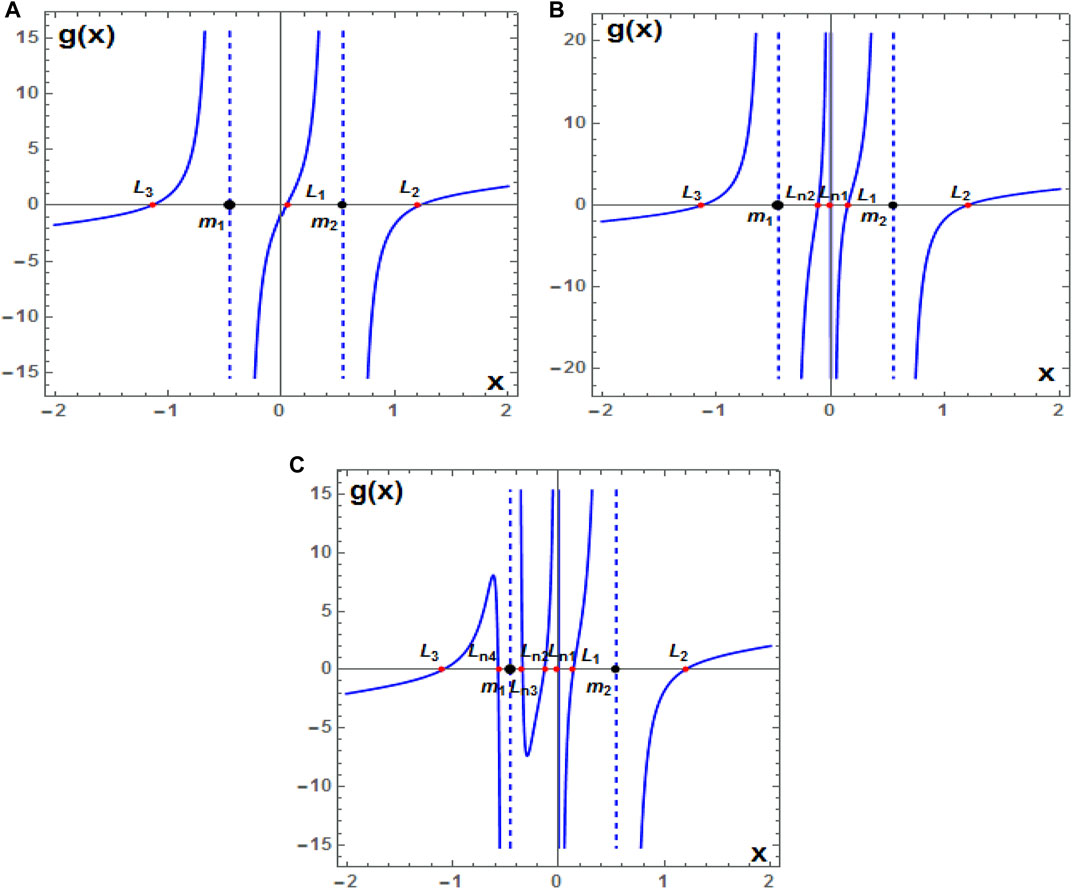
FIGURE 1. (A) Positions of the three collinear equilibrium points (red dots) L_i i = 1, 2, 3, for M_b = 0.00005. (B) Five collinear points L_i, i = 1, 2, 3, L_ni, i = 1, 2, for M_b = 0.05. In both frames, we have fixed μ = 0.455, σ₁ = 4 × 10⁻⁵, σ₂ = 3 × 10⁻⁵, σ₃ = 2 × 10⁻⁵, σ₄ = 10⁻⁵, A₃ = 0.02, T = 0.01, q₂ = 0.99, and q₁ = 0.8. (C) similar to panel (B), but for the case of seven collinear points in which σ₁ = 0.01, σ₂ = 0.03, σ₃ = 0.05, σ₄ = 0.07, and A₃ = 0.001. The positions of the primary bodies, m_i, i=1,2, are denoted by black dots.

We note that the triaxiality of the primaries has a high degree of complexity in a dynamical system, and any subtle changes in different parameters may substantially change the third body’s dynamic behavior (see, for e.g., Saeed and Zotos, 2021). The stability of the system equilibria is a significant problem for the understanding of the dynamical behaviors around these points. Based on the results given by Saeed and Zotos (2021), it can be predicted that the equilibria L_n3 and L_n4 are unstable. As a preliminary study, the discussions about these new equilibria resulting from triaxiality of the primaries will be ended by only examining the existence and stability of these points. Further studies can be made if needed, especially when these parameters are “pushed” at their limits.

Triangular Equilibrium Points (y ≠ 0)

For zero velocity and acceleration components in the equations of motion (Eq. 1) with y ≠ 0, the positions of the equilibria are the solutions of the nonlinear algebraic system U_x = U_y = 0, which yields:

$\begin{array}{l}{n}^{2}x-\frac{(1-\mu )(x+\mu )q_1}{r_1^3}-\frac{\mu q_2(x+\mu -1)}{r_2^3}-\frac{3(1-\mu )(2{\sigma }_1-{\sigma }_2)(x+\mu )q_1}{2r_1^5}\\ -\frac{3\mu q_2(2{\sigma }_1^{\prime }-{\sigma }_2^{\prime })(x+\mu -1)}{2r_2^5}+\frac{15(1-\mu )({\sigma }_1-{\sigma }_2)y^2{q}_1(x+\mu )}{2r_1^7}+\frac{15\mu ({\sigma }_1^{\prime }-{\sigma }_2^{\prime })y^2{q}_2(x+\mu -1)}{2r_2^7}\\ -\frac{3(1-\mu )(x+\mu )A_3}{2r_1^5}-\frac{3\mu (x+\mu -1)A_3}{2r_2^5}-\frac{M_{b}x}{{(r^2+T^2)}^{\frac{3}{2}}}=0,\end{array}(8)$

$\begin{array}{l}{n}^{2}y-\frac{\left(1-\mu \right)q_{1}y}{r_1^3}-\frac{\mu q_{2}y}{r_2^3}-\frac{3\left(1-\mu \right)\left(2{\sigma }_1-{\sigma }_2\right)q_{1}y}{2r_1^5}-\frac{3\left({\sigma }_1-{\sigma }_2\right)\left(1-\mu \right)q_{1}y}{r_1^5}-\frac{3\mu \left(2{\sigma }_1^{\prime }-{\sigma }_2^{\prime }\right)q_{2}y}{2r_2^5}\\ -\frac{3\left({\sigma }_1^{\prime }-{\sigma }_2^{\prime }\right)\mu q_{2}y}{r_2^5}+\frac{15\left(1-\mu \right)\left({\sigma }_1-{\sigma }_2\right)q_1{y}^3}{2r_1^7}\\ +\frac{15\mu \left({\sigma }_1^{\prime }-{\sigma }_2^{\prime }\right)q_2{y}^3}{2r_2^7}-\frac{3\left(1-\mu \right)A_{3}y}{2r_1^5}\\ -\frac{3\mu y{A}_3}{2r_2^5}-\frac{M_{b}y}{{\left(r^2+T^2\right)}^{\frac{3}{2}}}=0.\end{array}(9)$

The real solutions (x, y) of Eqs 8, 9 for those parameter values for which they exist provide the coordinates of the equilibrium points. Notice that

$U_x\left(x,-y;\mu ,q_1,q_2,{\sigma }_1,{\sigma }_2,{\sigma }_1^{\prime },{\sigma }_2^{\prime },A_3,M_b,T\right)=U_x\left(x,y;\mu ,q_1,q_2;{\sigma }_1,{\sigma }_2,{\sigma }_1^{\prime },{\sigma }_2^{\prime },A_3,M_b,T\right)$

and

$U_y\left(x,-y;\mu ,q_1,q_2,{\sigma }_1,{\sigma }_2,{\sigma }_1^{\prime },{\sigma }_2^{\prime },A_3,M_b,T\right)=-U_y\left(x,y;\mu ,q_1,q_2,{\sigma }_1,{\sigma }_2,{\sigma }_1^{\prime },{\sigma }_2^{\prime },A_3,M_b,T\right),$

and thus for each solution (x, y) of the equations with y > 0, (x, − y) is also a solution. So, the triangular equilibrium points come in pairs. Using the perturbation technique as that in Gyegwe et al. (2022), Eqs 8, 9 yield:

$\begin{array}{l}x=\frac{1}{2}-\mu -\frac{(1-q_1)}{3}+\frac{(1-q_2)}{3}-\frac{1}{2}(\frac{1}{\mu }-\frac{1}{4}){\sigma }_1+\frac{1}{2}(\frac{1}{\mu }+\frac{3}{4}){\sigma }_2+\frac{1}{2}(\frac{\mu }{1-\mu }+\frac{3}{4}){\sigma }_1^{\prime }-\frac{1}{2}(\frac{\mu }{1-\mu }+\frac{7}{4}){\sigma }_2^{\prime };\\ y=\pm \frac{\sqrt{3}}{2}\left[\begin{array}{l}1-\frac{2(1-q_1)}{9}-\frac{2(1-q_2)}{9}-\frac{4M_b(2rc-1)}{9{(r_c^2+T^2)}^{\frac{3}{2}}}+\\ \frac{1}{3}((\frac{-23}{4}+\frac{1}{\mu }){\sigma }_1+(\frac{19}{4}-\frac{1}{\mu }){\sigma }_2+(\frac{\mu }{1-\mu }-\frac{19}{4}){\sigma }_1^{\prime }+(\frac{15}{4}-\frac{\mu }{1-\mu }){\sigma }_2^{\prime }+2A_3)\end{array}\right],\end{array}(10)$

$0\mathrm{<}{M}_b,T,A_3,{\sigma }_i,{\sigma }_i^{\prime }\ll 1,i=\mathrm{1,2},$ Hence, Eq. 10 are the required coordinates of the triangular equilibrium points denoted by L_4,5 (x, ± y). It follows directly that the positions of the triangular points depend on the mass parameter μ and the perturbing forces involved in the equations of motion.

Moreover, we have verified these positions through numerical computations in which we plot in common diagram by making zero the equations of motion Eq. 1 in order to obtain the equilibria which appear as the intersection points of the curves on the xy–plane. In Figure 2, we show as a matter of interest, the location of the collinear and triangular equilibrium points as well as the fixed location of the primaries resulting from the solutions of Eq. 1 for the parameter values μ = 0.4583, M_b = 0.05, σ₁ = 4 × 10⁻⁵, σ₂ = 3 × 10⁻⁵, σ₃ = 2 × 10⁻⁵, σ₄ = 10⁻⁵, A₃ = 0.02, T = 0.01, q₂ = 0.99, and q₁ = 0.8. Black dots represent primaries, red dots stand for the equilibrium points, and blue curves and orange curves represent the curves U_x = 0 and U_y = 0, respectively. Moreover, our numerical computations (not shown here for latter studies) suggest the influence of triaxiality parameters of the primaries by revealing additional cases, regarding the total number of noncollinear equilibria, especially when these parameters are “pushed” at their limits. Detailed discussions can be made in terms of the variation of such parameters in further studies if needed.

FIGURE 2

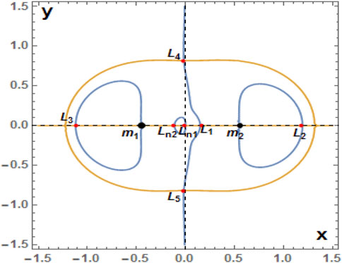
FIGURE 2. Plots of U_x = 0 (blue curves) and U_y = 0 (orange curves) depicting the locations of the seven equilibrium points (red dots) on the x y–plane for μ = 0.4583, M_b = 0.05, σ₁ = 4 × 10⁻⁵, σ₂ = 3 × 10⁻⁵, σ₃ = 2 × 10⁻⁵, σ₄ = 10⁻⁵, A₃ = 0.02, T = 0.01, q₂ = 0.99, and q₁ = 0.8.

The Jacobian integral given by Eq. 6 for μ = 0.455 and ${\sigma }_i\mathrm{=}{\sigma }_i^{\prime }=0,i=\mathrm{1,2},M_b=A_3=0,q_1=q_2=1$ (gravitational case) provides the ZVCs and the corresponding surface shown in Figure 3A,B, respectively, in which the equilibria appear either as intercrossing points between two or more branches of the equipotential curves for a given C or as reducing points after a process of shrinking of closed zero-velocity curves when C varies. The infinitesimal particle is permitted to move inside the “chimney”-like infinitely high peaks at m₁ and m₂ where C tends to infinity and below it (Figure 3B).

FIGURE 3

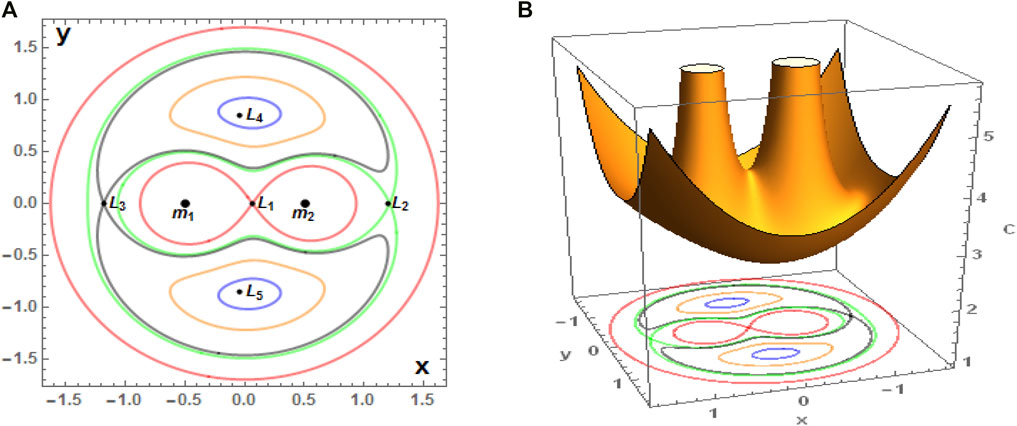
FIGURE 3. (Color figure online) (A) Zero-velocity curves for μ = 0.455, ${\sigma }_i={\sigma }_i^{\prime }=0$, i = 1, 2, M_b = A₃ = 0, q₁ = q₂ = 1, and Jacobi constant values: $C=C_{L_1}$ (red line), $C=C_{L_2}$ (green line), C = C_L3 (black line), C = 3 (yellow line), and C = 2.8 (blue line). The two primary bodies are denoted by m_i i = 1, 2, while the five equilibrium points L_i, i = 1,...,5, are indicated by small circles. (B) Surface and the corresponding zero-velocity curves of the problem in the gravitational case.

Stability of Collinear and Triangular Points

We investigate the linear stability of the infinitesimal motions when small displacements ξ and η are given to the coordinates of an equilibrium point (x₀, y₀) such that:

$\xi =x-x_0,\eta =y-y_0.(11)$

Substituting these values in system Eq. 1, we obtain the linearized system:

$\begin{array}{l}\ddot{\xi }-2n\dot{\eta }=U_{xx}^{\left(0\right)}\xi +U_{xy}^{\left(0\right)}\eta ,\\ \ddot{\eta }+2n\dot{\xi }=U_{xy}^{\left(0\right)}\xi +U_{yy}^{\left(0\right)}\eta .\end{array}(12)$

Here, only linear terms in ξ and η have been taken. The second partial derivatives of U are denoted by subscripts, while the superscript “0” indicates that the derivatives are to be evaluated at the equilibrium point (x₀, y₀). Now, the characteristic equation of the linearized system Eq. 12 is:

${\lambda }^4+\left(4n^2-U_{xx}^{\left(0\right)}-U_{yy}^{\left(0\right)}\right){\lambda }^2+U_{xx}^{\left(0\right)}{U}_{yy}^{\left(0\right)}-{\left[U_{xy}^{\left(0\right)}\right]}^2=0.(13)$

For the collinear equilibrium points $U_{xy}^{\left(0\right)}=U_{yx}^{\left(0\right)}=0$, and stability occurs when all four roots of the characteristic equation for λ are pure imaginary or complex roots all of which have negative real parts. This happens if the following three necessary as well as sufficient conditions are satisfied simultaneously:

${\left[4n^2-U_{xx}^{\left(0\right)}-U_{yy}^{\left(0\right)}\right]}^2-4U_{xx}^{\left(0\right)}{U}_{yy}^{\left(0\right)}>0,4n^2-U_{xx}^{\left(0\right)}-U_{yy}^{\left(0\right)}>0,U_{xx}^{\left(0\right)}{U}_{yy}^{\left(0\right)}>0.(14)$

In all other cases, the equilibrium points are unstable. In the present problem, the collinear points L_{1,2,3,n2,n3,n4} with respect to mass parameter μ and relative to involved perturbing forces are unstable since Eq. 13 has two real eigenvalues λ_1,2 = ±a and two imaginary eigenvalues λ_3,4 = ±ib, while the point L_n1 is stable since the conditions (Eq. 14) are satisfied simultaneously, i.e., Eq. 13 has four purely imaginary eigenvalues of the form λ_1,2 = ±ia, λ_3,4 = ± ib. Studying the stability of the collinear equilibria for the specific values μ = 0.455, σ₁ = 0.01, σ₂ = 0.03, σ₃ = 0.05, σ₄ = 0.07, A₃ = 0.001, T = 0.01, M_b = 0.05, q₂ = 0.99, and q₁ = 0.8, we found that all the collinear equilibria are unstable except point L_n1, which is stable.

For the triangular equilibrium points, the characteristic equation is also given by Eq. 13 but now $U_{xy}^{\left(0\right)}=U_{yx}^{\left(0\right)}\ne 0,$ so the corresponding inequalities for purely imaginary roots are given by:

${\left(4n^2-U_{xx}^{\left(0\right)}-U_{yy}^{\left(0\right)}\right)}^2-4\left[U_{xx}^{\left(0\right)}{U}_{yy}^{\left(0\right)}-{\left(U_{xy}^{\left(0\right)}\right)}^2\right]>0,4n^2-U_{xx}^{\left(0\right)}-U_{yy}^{\left(0\right)}>0,U_{xx}^{\left(0\right)}{U}_{yy}^{\left(0\right)}-{\left[U_{xy}^{\left(0\right)}\right]}^2>0.(15)$

Now, at the triangular points which are given by Eq. 10, we have the following analytical formulas depending only on the parameters of the problem:

$\begin{array}{l}{U}_{xy}^{\left(0\right)}=U_{yx}^{\left(0\right)}=\frac{3\sqrt{3}}{2}\left\{\begin{array}{l}\frac{1}{2}-\mu -\left[\frac{1}{9}+\frac{\mu }{9}\right]\left(1-q_1\right)+\left[\frac{2}{9}-\frac{\mu }{9}\right]\left(1-q_2\right)+\left[\frac{47}{24}-\frac{89\mu }{24}-\frac{1}{3\mu }\right]{\sigma }_1+\left[-\frac{3}{8}+\frac{37\mu }{24}+\frac{1}{3\mu }\right]{\sigma }_2+\\ \left[\frac{25}{12}-\frac{85\mu }{24}+\frac{\mu }{6\left(1-\mu \right)}+\frac{{\mu }^2}{6\left(1-\mu \right)}\right]{\sigma }_1^{\prime }+\left[-\frac{3}{2}+\frac{11\mu }{8}-\frac{\mu }{6\left(1-\mu \right)}-\frac{{\mu }^2}{6\left(1-\mu \right)}\right]{\sigma }_2^{\prime }+A_3\left(\frac{1}{3}-\frac{2\mu }{3}\right)\\ +\frac{M_b}{2}\left[\frac{11\left(2r_c-1\right)}{9{\left(r_c^2+T^2\right)}^{\frac{3}{2}}}+\frac{1}{{\left(r_c^2+T^2\right)}^{\frac{5}{2}}}\right]-\mu M_b\left[\frac{11\left(2r_c-1\right)}{9{\left(r_c^2+T^2\right)}^{\frac{3}{2}}}+\frac{1}{{\left(r_c^2+T^2\right)}^{\frac{5}{2}}}\right]\end{array}\right\},\\ U_{xx}^{\left(0\right)}=\frac{3}{4}-\left[\frac{1}{2}-\frac{3\mu }{2}\right](1-q_1)+\left[1-\frac{3\mu }{2}\right]\left(1-q_2\right)+\left[\frac{57}{16}+\frac{45\mu }{16}-\frac{3}{2\mu }\right]{\sigma }_1+\left[-\frac{3}{16}-\frac{93\mu }{16}+\frac{3}{2\mu }\right]{\sigma }_2\\ +\left[\frac{39}{8}-\frac{69\mu }{16}-\frac{3{\mu }^2}{2(1-\mu )}\right]{\sigma }_1^{\prime }+\left[-\frac{9}{2}+\frac{117\mu }{16}+\frac{3{\mu }^2}{2\left(1-\mu \right)}\right]{\sigma }_2^{\prime }+\frac{5M_b\left(2r_c-1\right)}{4{\left(r_c^2+T^2\right)}^{\frac{3}{2}}}+\frac{3M_b\left(\frac{1}{4}-\mu +{\mu }^2\right)}{{\left(r_c^2+T^2\right)}^{\frac{5}{2}}}\\ U_{yy}^{\left(0\right)}=\frac{9}{4}+3A_3+\left[\frac{1}{2}-\frac{3\mu }{2}\right]\left(1-q_1\right)-\left[1-\frac{3\mu }{2}\right]\left(1-q_2\right)+\left[\frac{87}{16}-\frac{45\mu }{16}+\frac{3}{2\mu }\right]{\sigma }_1+\left[-\frac{21}{16}+\frac{45\mu }{16}-\frac{3}{2\mu }\right]{\sigma }_2\\ +\left[\frac{33}{8}+\frac{135\mu }{16}-\frac{33\mu }{8\left(1-\mu \right)}+\frac{45{\mu }^2}{8\left(1-\mu \right)}\right]{\sigma }_1^{\prime }+\left[-\frac{135\mu }{16}+\frac{33\mu }{8\left(1-\mu \right)}-\frac{45{\mu }^2}{8\left(1-\mu \right)}\right]{\sigma }_2^{\prime }\\ +\frac{7M_b\left(2r_c-1\right)}{4{\left(r_c^2+T^2\right)}^{\frac{3}{2}}}+\frac{9M_b}{4{\left(r_c^2+T^2\right)}^{\frac{5}{2}}}\end{array}(16)$

Substituting these values in Eq. 13, the characteristic equation after normalizing becomes:

${\lambda }^4+b_1{\lambda }^2+b_2=0,(17)$

where we have abbreviated,

$b_1=4n^2-U_{xx}^{\left(0\right)}-U_{yy}^{\left(0\right)},b_2=U_{xx}^{\left(0\right)}{U}_{yy}^{\left(0\right)}-U_{yx}^{\left(0\right)}{U}_{xy}^{\left(0\right)},(18)$

with

$b_1=1-3A_3+3{\sigma }_1+\left(-\frac{9}{2}+3\mu \right){\sigma }_2+3{\sigma }_1^{\prime }-3\left(\mu +\frac{1}{2}\right){\sigma }_2^{\prime }+\frac{M_b\left(2r_c+3\right)}{{\left(r_c^2+T^2\right)}^{\frac{3}{2}}}-\frac{3M_b{r}_c^2}{{\left(r_c^2+T^2\right)}^{\frac{5}{2}}},$

$\begin{array}{l}{b}_2=\mu (1-\mu )\left[\frac{27}{4}+\frac{3}{2}(1-q_1)+\frac{3}{2}(1-q_2)+9A_3\right]-\left[\frac{45}{8}-\frac{891\mu }{16}+\frac{801{\mu }^2}{16}\right]{\sigma }_1\\ +\left[\frac{45}{8}-\frac{423\mu }{16}+\frac{333{\mu }^2}{16}\right]{\sigma }_2+\left[\frac{711\mu }{16}-\frac{801{\mu }^2}{16}\right]{\sigma }_1^{\prime }-\left[\frac{243\mu }{16}-\frac{333{\mu }^2}{16}\right]{\sigma }_2^{\prime }\\ +\frac{33\mu (1-\mu )(2r_c-1)M_b}{2{(r_c^2+T^2)}^{\frac{3}{2}}}+\frac{27\mu (1-\mu )M_b}{4{(r_c^2+T^2)}^{\frac{5}{2}}}.\end{array}$

Its roots are:

${\lambda }^2=\frac{-b_1\pm \sqrt{\mathrm{\Delta }}}{2},(19)$

where the discriminant Δ which defines the nature of roots is expressed as:

$\begin{array}{l}\mathrm{\Delta }=b_1^2-4b_2\\ ={\mu }^2\left(27+36A_3+6\left(1-q_1\right)+6\left(1-q_2\right)+\frac{801}{4}\left({\sigma }_1+{\sigma }_1^{\prime }\right)-\frac{333}{4}\left({\sigma }_2+{\sigma }_2^{\prime }\right)+\frac{66M_b(2r_c-1)}{{\left(r_c^2+T^2\right)}^{\frac{3}{2}}}+\frac{27M_b}{{\left(r_c^2+T^2\right)}^{\frac{5}{2}}}\right)\\ -\mu \left(27+36A_3+6\left(1-q_1\right)+6\left(1-q_2\right)+\frac{891}{4}{\sigma }_1-\frac{447}{4}{\sigma }_2+\frac{711}{4}{\sigma }_1^{\prime }-\frac{219}{4}{\sigma }_2^{\prime }+\frac{66M_b\left(2r_c-1\right)}{{\left(r_c^2+T^2\right)}^{\frac{3}{2}}}+\frac{27M_b}{{\left(r_c^2+T^2\right)}^{\frac{5}{2}}}\right)\\ +1-6A_3+\frac{57}{2}{\sigma }_1-\frac{63}{2}{\sigma }_2+6{\sigma }_1^{\prime }-3{\sigma }_2^{\prime }+\frac{2M_b\left(2r_c+3\right)}{{\left(r_c^2+T^2\right)}^{\frac{3}{2}}}-\frac{6M_b{r}_c^2}{{\left(r_c^2+T^2\right)}^{\frac{5}{2}}}\end{array}$

Now

${\left(\mathit{\Delta }\right)}_{\mu =0}=1-6A_3+\frac{57}{2}{\sigma }_1-\frac{63}{2}{\sigma }_2+6{\sigma }_1^{\prime }-3{\sigma }_2^{\mathit{\text{'}}}+\frac{2M_b\left(2r_c+3\right)}{{\left(r_c^2+T^2\right)}^{\frac{3}{2}}}-\frac{6M_b{r}_c^2}{{\left(r_c^2+T^2\right)}^{\frac{5}{2}}}>0,$

and

$\begin{array}{l}{\left(\mathit{\Delta }\right)}_{\mu =\frac{1}{2}}=-\frac{23}{4}-15A_3-\frac{3}{2}\left(1-q_1\right)-\frac{3}{2}\left(1-q_2\right)-\frac{565}{16}{\sigma }_1+\frac{57}{16}{\sigma }_2-\frac{525}{16}{\sigma }_1^{\mathit{\text{'}}}+\frac{57}{16}{\sigma }_2^{\mathit{\text{'}}}-\frac{33M_b\left(2r_c-1\right)}{2{\left(r_c^2+T^2\right)}^{\frac{3}{2}}}\\ +\frac{2M_b\left(2r_c+3\right)}{{\left(r_c^2+T^2\right)}^{\frac{3}{2}}}-\frac{27M_b}{4{\left(r_c^2+T^2\right)}^{\frac{5}{2}}}-\frac{6M_b{r}_c^2}{{\left(r_c^2+T^2\right)}^{\frac{5}{2}}}<0.\end{array}$

Evidently, the values of Δ when $\mu =0$ and $\mu =\frac{1}{2}$ have opposite signs. Hence, there is a value of $\mu$ in the interval $0\le \mu \le \frac{1}{2}$ at which Δ = 0 is called the critical mass parameter denoted by μ_crit. Hence, we solve Δ = 0 for $\mu$ and simplify to finally get:

${\mu }_{crit}={\mu }_o+{\mu }_b+{\mu }_r+{\mu }_t+{\mu }_d,(20)$

with

$\begin{array}{l}{\mu }_o=\frac{1}{2}\left(1-\sqrt{\frac{23}{27}}\right);{\mu }_b=-\frac{22A_3}{9\sqrt{69}};{\mu }_r=-\frac{2}{27\sqrt{69}}\left[\left(1-q_1\right)+\left(1-q_2\right)\right],\\ {\mu }_t=\left(\frac{5}{12}+\frac{59}{18\sqrt{69}}\right){\sigma }_1-\left(\frac{19}{36}+\frac{85}{18\sqrt{69}}\right){\sigma }_2-\left(\frac{5}{12}-\frac{59}{18\sqrt{69}}\right){\sigma }_1^{\prime }+\left(\frac{19}{36}-\frac{85}{18\sqrt{69}}\right){\sigma }_2^{\prime },\\ {\mu }_d=\frac{\left(76-8r_c\right)M_b}{27\sqrt{69}{\left(r_c^2+T^2\right)}^{\frac{3}{2}}}-\frac{\left(1+6r_c^2\right)M_b}{3\sqrt{69}{\left(r_c^2+T^2\right)}^{\frac{5}{2}}}.\end{array}(21)$

Equation 20 represents the perturbed critical mass ratio with five parts (i.e., in terms of all the perturbing parameters). The first part μ₀ represents the classical case without perturbation, the second part μ_b is related to the oblate infinitesimal body, the third part μ_r is related to radiation pressure of the primaries, and the fourth part μ_t is connected to the triaxiality of the primaries, while the fifth part μ_d is related to the circular cluster of material points. Therefore, it is clearly observed that stability regions depend on the perturbing forces of our model. We remark that for M_b = 0, the results agree fully with previously published results (see Gyegwe et al., 2022 and references therein), while in case where ${\sigma }_i\mathrm{=}{\sigma }_i^{\prime }=0,i=1,2,$ our results coincide with those by Amuda et al. (2021).

There are three cases (1–3) to determine the linear stability of the triangular equilibrium points. 1) When 0 < μ <μ_crit, Δ > 0, the roots Eq. 19 are distinct pure imaginary numbers, and the solution is bounded. Hence, the triangular points are stable in this region. 2) When ${\mu }_{crit}<\mu \le \frac{1}{2},$ Δ < 0, then the real parts of two of the roots (Eq. 19) are positive and the triangular points are unstable. 3) When μ = μ_crit, Δ = 0, then the roots in Eq. 19 are double which leads to instability of the triangular points. Therefore, we established that the triangular points are stable only for 0 < μ < μ_crit and unstable for μ_crit ≤ μ ≤ = 1/2. Hence, the stability region is:

$\begin{array}{l}0<\mu <{\mu }_{crit}={\mu }_o-\frac{22A_3}{9\sqrt{69}}-\frac{2}{27\sqrt{69}}[(1-q_1)+(1-q_2)]+\left(\frac{5}{12}+\frac{59}{18\sqrt{69}}\right){\sigma }_1-\left(\frac{19}{36}+\frac{85}{18\sqrt{69}}\right){\sigma }_2\\ -\left(\frac{5}{12}-\frac{59}{18\sqrt{69}}\right){\sigma }_1^{\prime }+\left(\frac{19}{36}-\frac{85}{18\sqrt{69}}\right){\sigma }_2^{\prime }+\frac{(76-8r_c)M_b}{27\sqrt{69}{\left(r_c^2+T^2\right)}^{\frac{3}{2}}}-\frac{(1+6r_c^2)M_b}{3\sqrt{69}{\left(r_c^2+T^2\right)}^{\frac{5}{2}}},\end{array}$

where ${\mu }_o=\frac{1}{2}\left(1-\sqrt{\frac{23}{27}}\right)\approx 0.03852089$ is Routh’s critical value.

This critical mass parameter value gives the measure of the size of the stability region. Computations of Eq. 20 clearly reveal that the critical mass ratio decreases with the increase in the values of the radiation pressure, triaxiality, and oblate infinitesimal body, as shown in Gyegwe et al. (2022); however, it increases with the increase in the value of mass of the disc. It is noticed that all three of the former and the latter one possess destabilizing and stabilizing behavior, respectively. Moreover, under the combined effect of the parameters, the size of the region of stability decreases with a simultaneous increase in the values of the parameters. Remarkably, the present results of the triangular points are in conformity with Yeh and Jiang (2006) for q_i = 1,  i = 1, 2, A₃ = 0, and ${\sigma }_i\mathrm{=}{\sigma }_i^{\prime }=0,i=\mathrm{1,2},$ in the present work and for M_b = 0, also agree with those of Gyegwe et al. (2022) and references therein; the difference in configuration of the primary bodies is responsible for the difference in sign.

Numerical Application

In this section, we apply the data of the binary HD155876 system given in Table 1 to the results obtained in our previous sections (Singh et al., 2018). The influence of the involved perturbations on the zero-velocity surface and the positions of the collinear and triangular points will be studied in this section. The numbering of the equilibrium points and the relative positions of the primaries are illustrated according to the diagram shown in Figure 2 for the same mass ratio (μ = 0.4583) of the primaries. Eq. 10 has been used to compute the coordinates of the triangular points.

TABLE 1

TABLE 1. Numerical data for the binary HD155876 system (Singh et al., 2018).

Effects of the Perturbations on the Zero -Velocity Surfaces

We plot in Figure 4 the zero-velocity surface Eq. 6 for the HD155876 binary system for the purely gravitational case and five different cases of the involved parameters: Panel (A) is for the gravitational case, panel (B) shows the oblateness effect of the third body, panel (C) shows the effect of enclosed material points in which the immediate formation of a new “chimney” around the bigger primary is obvious, panel (D) shows the effect of triaxiality of the bigger primary, panel (E) shows the effect of triaxiality of the smaller primary, and panel (F) shows the effect of the radiation coefficients of the binary system, while panel (G) shows the combine effects of triaxiality and radiation pressure of both primaries, oblateness of the third body, and enclosed material points of the primaries. From these frames, we can observe two main results. The first is a change of the Jacobian constants, which correspond to all equilibrium points with or without involved parameters due to which results of zero-velocity surfaces show the chaotic behavior. Note the different values of the Jacobian constant C of the panels (B)–(G) w.r.t panel (A). The second is a shrinking or enlargement of the “chimneys” around each primary which limit the area of the permitted third body’s motion in the neighborhood of the two primaries for each of the panels (B)–(G) w.r.t panel (A). We note two collinear equilibria which emerge on side of primary body $m_1,$ in addition to the three classical points [see panels (C) and (G)]. It is also remarkable that for a given value of the Jacobian constant C and as the involved parameters increase, the allowed regions of the third body motion around the two bodies expand [panel (G)]. This means that the third body can move freely around the primaries for bigger and bigger values of the Jacobian constant C as the parameters increase.

FIGURE 4

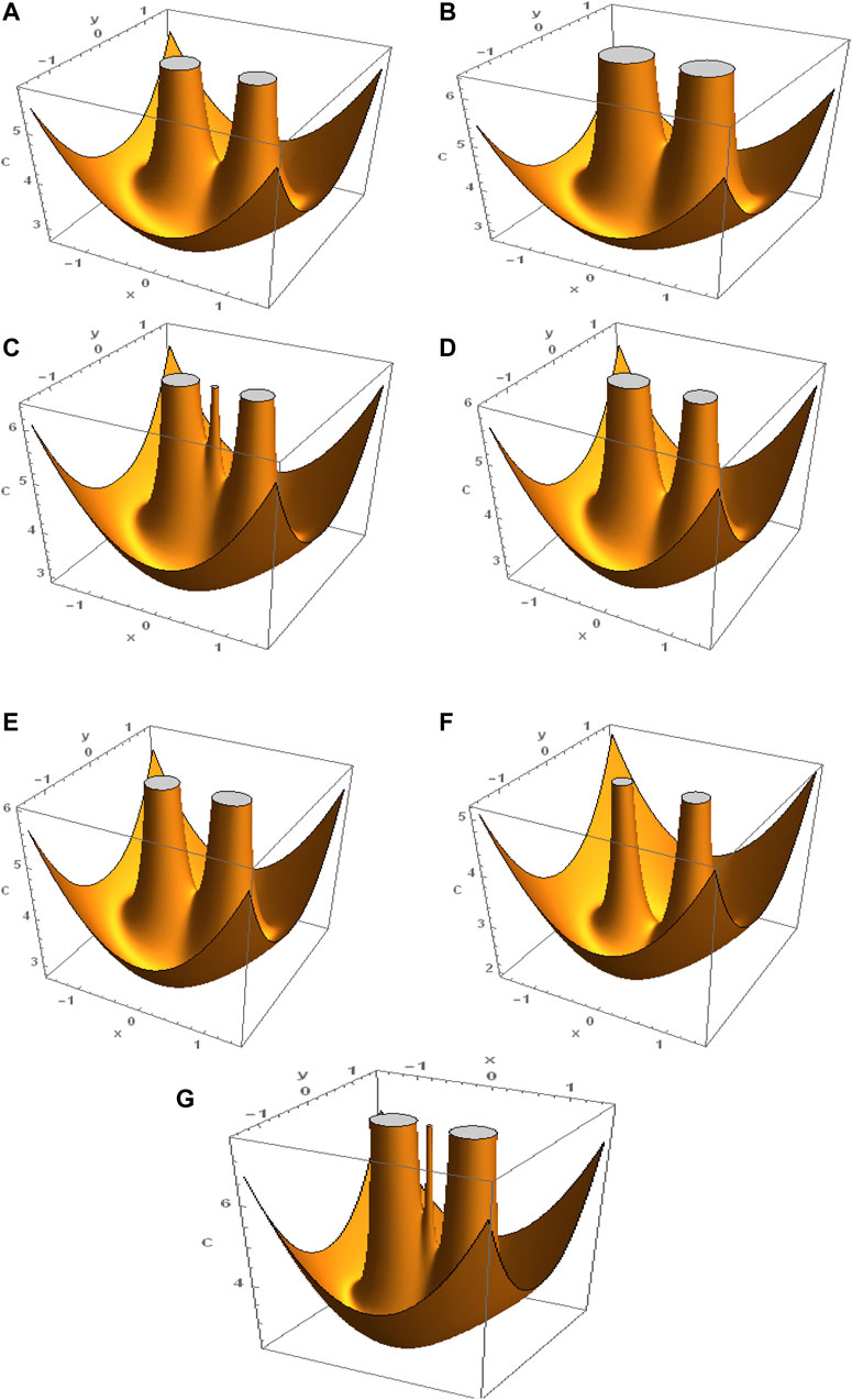
FIGURE 4. (Color figure online) Zero-velocity surfaces of the HD155876 (μ = 0.4583) binary system for (A) A₃ = 0, σ₁ = σ₂ = 0, ${\sigma }_1^{\prime }={\sigma }_2^{\prime }=0$, M_b = 0, and q₁ = q₂ = 1 (classical case); (B) A₃ = 0.09, σ₁ = σ₂ = 0, ${\sigma }_1^{\prime }={\sigma }_2^{\prime }=0$, M_b = 0, and q₁ = q₂ = 1 case; (C) M_b = 0.05, T = 0.01, A₃ = 0, σ₁ = σ₂ = 0, ${\sigma }_1^{\prime }={\sigma }_2^{\prime }=0$, and q₁ = q₂ = 1 case; (D) σ₁ = 0.02, σ₂ = 0.01, ${\sigma }_1^{\prime }={\sigma }_2^{\prime }=0$, A₃ = 0, M_b = 0, and q₁ = q₂ = 1 case; (E) ${\sigma }_1^{\prime }=0.02$, ${\sigma }_2^{\prime }=0.01$, σ₁ = σ₂ = 0, A₃ = 0, M_b = 0, and q₁ = q₂ = 1 case; (F) q₁ = 0.5, q₂ = 0.8, A₃ = 0, σ₁ = σ₂ = 0, ${\sigma }_1^{\prime }={\sigma }_2^{\prime }=0$, and M_b = 0 case; (G) q₁ = 0.45, q₂ = 0.75, A₃ = 0.1, σ₁ = 0.07, σ₂ = 0.05, ${\sigma }_1^{\prime }=0.03$, ${\sigma }_2^{\prime }=0.02$, M_b = 0.055, and T = 0.01 case. The presence of the new collinear points is obvious in panels (C) and (G). Motion is permitted inside the chimneys and below it. Note the different scales of Jacobian constant C in the first and the next frames.

It is obvious from these figures that the perturbing forces under consideration have a significant effect in which the motion of the test particle is allowed or forbidden in the vicinity of the HD155876 binary system, comparing the first frame with the six last ones. Remarkably, the cluster of material points of the primaries provides a new observation of its topological structure resulting in the neighborhood of $m_1$ primary a pair of new collinear equilibrium points. Here, we note that since the two primaries have unequal masses and unequal assumed model parameters, the two “chimneys” are asymmetric with respect to both (C, y) and (C, x) planes.

Influence of [q₁, q₂] on the Equilibria

For the arbitrary chosen values of the model parameters $A_3,{\sigma }_i,{\sigma }_i^{\prime },i=\mathrm{1,2},$ and M_b, the locations of the collinear and triangular equilibrium points are, respectively, presented in Tables 2 and 3 as a function of q₂ w.r.t. different values of q₁. Evidently, for fixed values of q₁ and increasing values of q₂, the coordinates x and y of the equilibria decrease or increase. Here, the increase or decrease is a measure of the deviation from the classical estimations. Specifically, with the increase of q₂, the collinear equilibrium positions L₂ and L₃ constantly shift their distance and move closer to the position where primary bodies $m_1$ and $m_2$ are located, correspondingly. L₁ and L_n1 go closer to $m_2$ and $m_1$, correspondingly, while at the same time collinear point L_n2 moves closer to the origin. At the same time, the two triangular points L₄ and L₅ decrease with the line connecting the two primaries.

TABLE 2

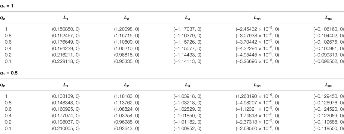
TABLE 2. Positions (x₀, 0) of the collinear points of the binary HD155876 system for the fixed values M_b = 0.05, T = 0.01, σ₁ = 4 × 10⁻⁵, σ₂ = 3 × 10⁻⁵, ${\sigma }_1^{\prime }=2\times {10}^{-5}$, ${\sigma }_2^{\prime }={10}^{-5}$, A₃ = 0.02, and for two fixed values of q₁ when q₂ radiates.

TABLE 3

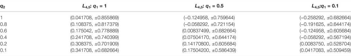
TABLE 3. Positions (x₀, ± y₀) of the triangular points of the binary HD155876 system for three fixed values of q₁ when q₂ radiates. The disc, oblateness, and triaxiality parameters are kept as constants as in the collinear case (Table 2).

Such a variational trend can also be seen from Figures 5 and 6 in which the equilibria positions have been marked with curves corresponding to the cases with q₁ = 1, q₁ = 0.5, and q₁ = 0.1 for the increasing values of radiation factor q₂ of the smaller primary. Here, we note from the tables and figures that the positions of L_n1, L₄, and L₅ are decreasing and increasing functions of q₂. A similar phenomenon is observed under the combined effects of q₁ and q₂ in which the positions of L_n1, L₄, and L₅ are monotonic functions of q₁ and q₂.

FIGURE 5

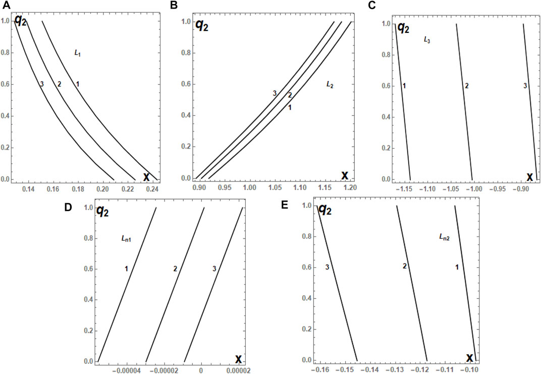
FIGURE 5. (A–E) Positions of the collinear equilibrium points L_i, i = 1, 2, 3, L_nj, j = 1, 2, of the HD11565 system, as a function of q₂, which varies in the interval (0, 1] for fixed values of q₁ equal to 1 (1), 0.5 (2), and 0.1 (3). The disc, oblateness, and triaxiality parameters are kept as constants as given in Table 2. The numbering of equilibrium points is according to the diagram shown in Figure 2.

FIGURE 6

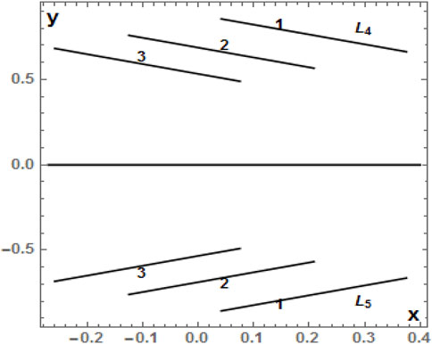
FIGURE 6. Positions of the two triangular equilibrium points L₄ and L₅ on the xy–plane as a function of q₂, which varies in the interval (0, 1] for fixed values of q₁ equal to 1 (1), 0.5 (2), and 0.1 (3). The disc, oblateness, and triaxiality parameters are kept as constants as given in Table 3.

Similarly, the locations of the collinear and triangular points are shown in Tables 4 and 5, respectively, as a function of q₁ with respect to different values of q₂. We observe that as the radiation coefficient q₂ increases for varying q₁, collinear equilibrium positions L₂ and L₃ decrease and move closer to the primaries $m_2$ and $m_1$, correspondingly, and points L_n1 and L_n2 both tend to $m_2$ and $m_1$, respectively, while point L₁ moves toward the origin. At the same time, the two triangular equilibria L₄ and L₅ go toward the line connecting the primaries as q₁ tends to zero for fixed values of q₂.

TABLE 4

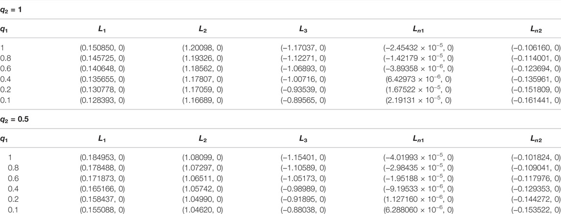
TABLE 4. Positions (x₀, 0) of the collinear points of the binary HD155876 system for fixed values M_b=0.05, T = 0.01, σ₁ = 4 × 10⁻⁵, σ₂ = 3 × 10⁻⁵, ${\sigma }_1^{\prime }=2\times {10}^{-5}$, ${\sigma }_2^{\prime }={10}^{-5}$, A₃ = 0.02, and for two fixed values of q₂ when q₁ radiates.

TABLE 5

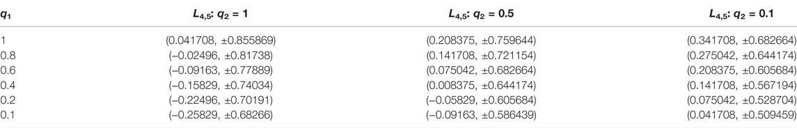
TABLE 5. Positions (x₀, ± y₀) of the triangular points of the binary HD155876 system for three fixed values of q₂ when q₁ radiates. The disc, oblateness, and triaxiality parameters are kept as constants as in the collinear case (Table 4).

Such a variational trend can also be seen from Figures 7 and 8 in which the equilibria positions have been marked with curves corresponding to the cases with q₂ = 1, q₂ = 0.5, and q₂ = 0.1 for values of the radiation factor of the bigger primary q₁ ∈ (0, 1]. We also observe from the tables and figures that the positions of L_n1, L₄, and L₅ are decreasing functions of q₁. A similar phenomenon is observe under the combined effects of q₁ and q₂ in which the positions of L_n1, L₄, and L₅ are monotonic functions of q₁ and q₂. It is also remarkable that under the combined effects of the radiation factors q₁ and q₂, the position (x, 0) of the equilibrium points L₁ and L_n2 is an increasing function and that of L₂ and L₃ is a decreasing function, while the x coordinate of L_n1, L₄, and L₅ is a monotonic function of q₁ and q₂ (Tables 4, 5 and Figures 7, 8).

FIGURE 7

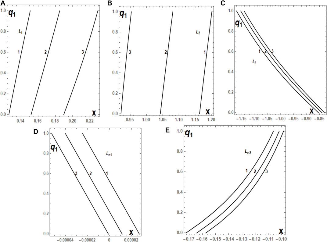
FIGURE 7. (A–E) Positions of the collinear equilibria L_i, i = 1, 2, 3, L_nj, j = 1, 2, of the HD11565 system, as a function of q₁, which varies in the interval (0, 1] for fixed values of q₂ equal to 1 (1), 0.5 (2), and 0.1 (3), respectively. The disc, oblateness, and triaxiality parameters are kept as constants as given in Table 4. The numbering of equilibrium points is according to the diagram shown in Figure 2.

FIGURE 8

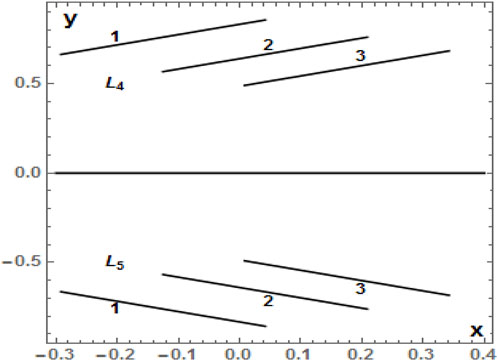
FIGURE 8. Positions of the two triangular equilibrium points L₄ and L₅ on the xy–plane as a function of q₁, which varies in the interval (0, 1] for fixed values of q₂ equal to 1 (1), 0.5 (2), and 0.1 (3). The disc, oblateness, and triaxiality parameters are kept as constants as given in Table 5.

Influence of [A₃, M_b] on the Equilibria

In order to analyze the effects of oblate infinitesimal mass A₃ and mass of the disc M_b, we have obtained the coordinates of the five collinear and the two triangular equilibria for varying oblateness and varying mass of the disc at fixed values of q₁, q₂, σ₁, σ₂, ${\sigma }_1^{\prime }$, and ${\sigma }_2^{\prime }$ (Tables 6, 7). From the results presented in Table 6, it is clear that with an increase in the value of A₃ for fixed values of M_b, points L₂ and L₃ tend to infinity (L₂ → ∞, L₃ → − ∞), and L₁ and L_n2 tend closest to the origin, while the inner point L_n1 tends to the position of $m_1,$ correspondingly. On the other hand, with an increase in the value of A₃ for fixed values of M_b, the two triangular points L₄ and L₅ both tend to infinity (L₄ → ∞, L₅ → − ∞) (Table 7).

TABLE 6

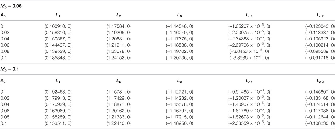
TABLE 6. Positions (x₀, 0) of the collinear points of the binary HD155876 system for fixed values q₁ = 0.979950, q₂ = 0.983912, T = 0.01, σ₁ = 4 × 10⁻⁵, σ₂ = 3 × 10⁻⁵, ${\sigma }_1^{\prime }=2\times {10}^{-5}$, ${\sigma }_2^{\prime }={10}^{-5}$, and for two fixed values of M_b when the value of A₃ varies.

TABLE 7

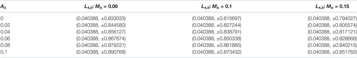
TABLE 7. Positions (x₀, ±y₀) of the two triangular points L₄ and L₅ of the binary HD155876 system for three fixed values of M_b when A₃ varies. The radiation pressure and triaxiality parameters are kept as constants as in the collinear case (Table 6).

Such variational trends for graphical solutions of the collinear and triangular equilibria are shown in Figures 9 and 10, respectively. From Tables 6 and 7, it is clearly seen that for fixed values of A₃ and varying values of M_b, points L₁ and L₂ move closest to the position of $m_2,$ L₃ and L₁ tend to the position of $m_1,$ and L₁ moves closer to the origin, while L₄ and L₅ tend to the line joining the primaries. Due to the limiting space of the article, we do not present here this case as the presentation is obvious with regard to the previous case. Moreover, in the absence and presence of the remaining parameters, changes in the value of M_b or A₃ do not influence the x-coordinates of the triangular points analytically (Table 7 and Figure 10). However, under the joint action of both parameters, the situation is analogous for variation of M_b and fixed values of A₃. This indicates that the presence of the disc plays a certain degree of “correction” to the two primaries’ dynamic behavior, so that they can maintain regular motion as much as possible.

FIGURE 9

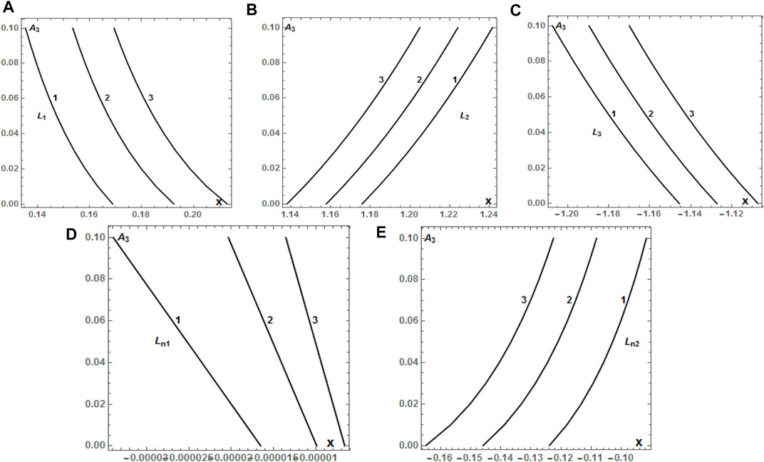
FIGURE 9. (A–E) Positions of the collinear equilibrium points L_i, i = 1, 2, 3, L_nj, j = 1, 2, of the HD155876 system, as a function of A₃, which varies in the interval (0, 0.1] for fixed values of M_b equal to 0.06 (1), 0.1 (2), and 0.15 (3), respectively. The radiation pressure and triaxiality parameters are kept as constants as in the previous case (Table 6). The numbering of equilibrium points is according to the diagram shown in Figure 2.

FIGURE 10

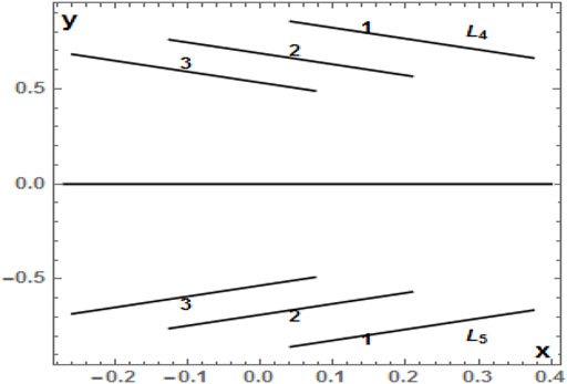
FIGURE 10. Positions of the two triangular equilibrium points L₄ and L₅ on the xy–plane as a function of A₃, which varies in the interval (0, 0.1) for fixed values of M_b equal to 0.06 (1), 0.1 (2), and 0.15 (3). The radiation pressure and triaxiality parameters are kept as constants as in Table 7.

Influence of Triaxiality of the Bigger Primary (σ₁, σ₂) on the Equilibria

Tables 8 and 9 evaluate triaxiality effects of the bigger primary in the binary system on the collinear and triangular equilibrium points, respectively, while in Figures 11 and 12, we summarize these effects on their positions, respectively. Evidently, an increase in the value of σ₁ for fixed values of σ₂, points L₁ and L₂ tend toward the smaller primary m₂, L_n1 and L_n2 approach each other, while L₃ tends to minus infinity, whereas the two triangular points L₄ and L₅ both tend to the Ox–axis.

TABLE 8

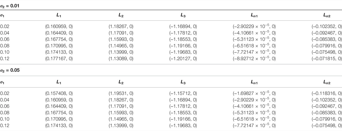
TABLE 8. Positions (x₀, 0) of the collinear points of the binary HD155876 system for fixed values q₁ = 0.979950, q₂ = 0.983912, A₃ = 0.02, M_b = 0.06, T = 0.01, ${\sigma }_1^{\prime }=2\times {10}^{-5}$, ${\sigma }_2^{\prime }={10}^{-5}$, and for two fixed values of ${\sigma }_2$ when ${\sigma }_1$ varies.

TABLE 9

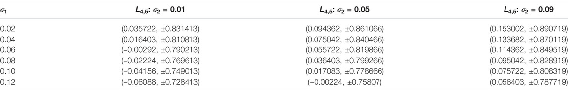
TABLE 9. Positions (x₀, ± y₀) of the two triangular points L₄ and L₅ of the binary HD155876 system for three fixed values of σ₂ when σ₁ varies. The radiation pressure, oblateness, mass of the disc, and triaxiality parameters of the smaller primary are kept as constants as in the collinear case (Table 8).

FIGURE 11

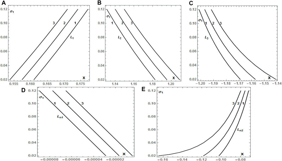
FIGURE 11. (A–E) Positions of the collinear equilibrium points L_i, i = 1, 2, 3, L_nj, j = 1, 2, of the HD155876 system, as a function of σ₁, which varies in the interval (0.02, 0.12) for fixed values of σ₂ equal to 0.01 (1), 0.05 (2), and 0.09 (3), respectively. The radiation pressure, oblateness, mass of the disc, and triaxiality parameters of the smaller primary are kept as constants as in the previous case (Table 8). The numbering of equilibrium points is according to the diagram shown in Figure 2.

FIGURE 12

FIGURE 12. Positions of the two triangular equilibrium points L₄ and L₅ on the xy–plane as a function of σ₁, which varies in the interval (0.02, 0.12) for fixed values of σ₂ equal to 0.01 (1), 0.05 (2) and 0.09 (3). The radiation pressure, oblateness, mass of the disc, and triaxiality parameters of the smaller primary are kept as constants as in the previous case (Table 9).

Influence of Triaxiality of the Smaller Primary (${\mathit{\sigma }}_1^{\prime },{\mathit{\sigma }}_2^{\prime }$) on the Equilibria

Tables 10 and 11evaluate triaxiality effects of the smaller primary in the binary system on the collinear and triangular equilibrium points, respectively, while in Figures 13 and 14, we summarize these effects on their positions, respectively. Evidently, an increase in the value of ${\sigma }_1^{\prime }$ for fixed values of ${\sigma }_2^{\prime }$, points L₁ and L_n1 both tend toward the origin, L₃ and L_n2 both approach the bigger primary m₁, while L₂ tends to plus infinity, whereas the two triangular points L₄ and L₅ both move toward the Ox–axis.

TABLE 10

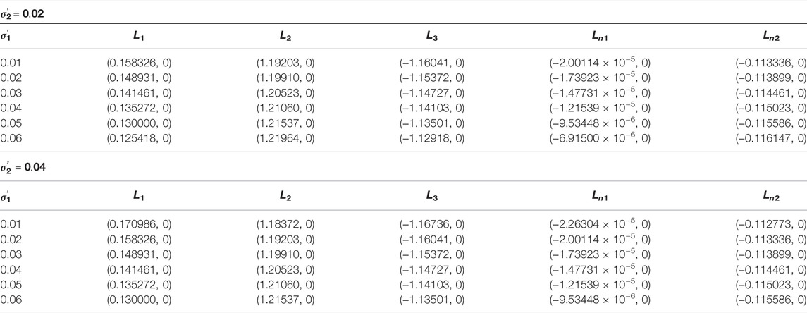
TABLE 10. Positions (x₀, 0) of the collinear points of the binary HD155876 system for fixed values q₁ = 0.979950, q₂ = 0.983912, A₃ = 0.02, M_b = 0.06, T = 0.01, σ₁ = 4 × 10⁻⁵, σ₂ = 3 × 10⁻⁵, and for two fixed values of ${\sigma }_2^{\prime }$ when ${\sigma }_1^{\prime }$ varies.

TABLE 11

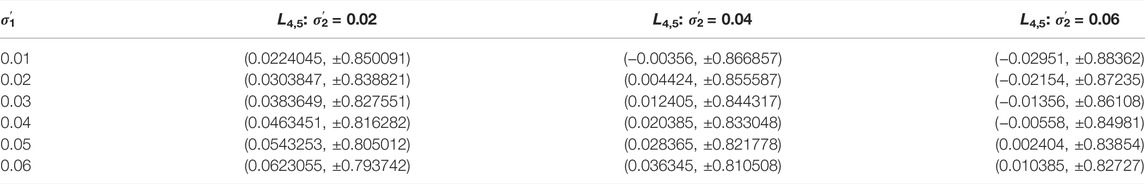
TABLE 11. Positions (x₀, ±y₀) of the two triangular points L₄ and L₅ of the binary HD155876 system for three fixed values of ${\sigma }_2^{\prime }$ when ${\sigma }_1^{\prime }$ varies. The radiation pressure, oblateness, mass of the disc, and triaxiality parameters of the bigger primary are kept as constants as in the collinear case (Table 10).

FIGURE 13

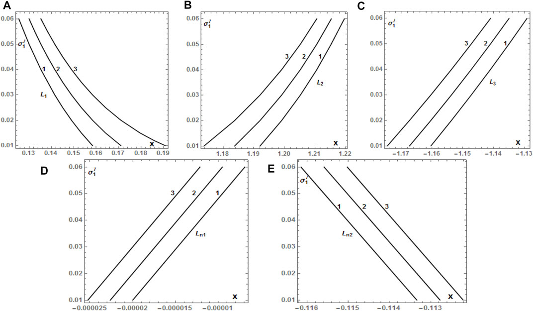
FIGURE 13. (A–E) Positions of the collinear equilibrium points L_i, i = 1, 2, 3, L_nj, j = 1, 2, of the HD155876 system, as a function of ${\sigma }_1^{\prime }$, which varies in the interval (0.01, 0.06) for fixed values of ${\sigma }_2^{\prime }$ equal to 0.02 (1), 0.04 (2), and 0.06 (3), respectively. The radiation pressure, oblateness, mass of the disc, and triaxiality parameters of the bigger primary are kept as constants as in the previous case (Table 10). The numbering of equilibrium points is according to the diagram shown in Figure 2.

FIGURE 14

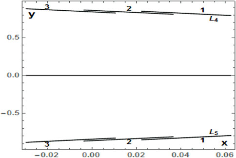
FIGURE 14. Positions of the two triangular equilibrium points L₄ and L₅ on the xy–plane as a function of ${\sigma }_1^{\prime }$, which varies in the interval (0.01, 0.06) for fixed values of ${\sigma }_2^{\prime }$ equal to 0.02 (1), 0.04 (2), and 0.06 (3). The radiation pressure, oblateness, mass of the disc, and triaxiality parameters of the bigger primary are kept as constants as in the previous case (Table 11).

Now, we shall analyze the linear stability of the collinear and triangular equilibrium points by looking at the eigenvalues of the characteristic Eq. 13. In this article, for a particular example, we compute the stability of the collinear and triangular points under the joint effect of oblate infinitesimal body and mass of the disc of the binary system HD155876 when the remaining parameters q₁, q₂, σ₁, σ₂, ${\sigma }_1^{\prime }$, and ${\sigma }_2^{\prime }$ are fixed. The results are summarized in Table 12 in which the presence of positive real roots or positive real part in complex roots affirms the instability of L_1,2,3,n2 and L₄₍₅₎ of the problem when applied to the HD155876 system. However, for point L_n1, we get all purely imaginary roots implying that due to all imaginary roots at this point are stable.

TABLE 12

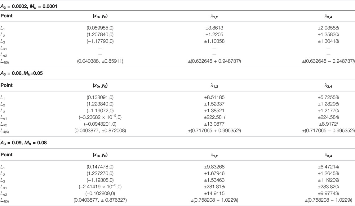
TABLE 12. Locations and eigenvalues λ_1,2, λ_3,4 of Eq. 13 in the HD155876 binary system with varying oblateness and mass of the disc for q₁ = 0.979950, q₂ = 0.983912, σ₁ = 4 × 10⁻⁵, σ₂ = 3 × 10⁻⁵, ${\sigma }_1^{\prime }=2\times {10}^{-5}$, and ${\sigma }_2^{\prime }={10}^{-5}$.

Discussion and Conclusion

Following the equations of motion of an oblate body with negligible mass moving under the gravitational attraction of radiating primaries coupled with triaxiality of the two stars together with a circular cluster of materials, we determined the positions of the collinear and triangular equilibrium points. The resulting equations of motion differ from those described by Gyegwe et al. (2022) due to the potential from the belt. It was observed that the positions of these points are affected by the mass parameter and perturbing forces involved in the equations of motion. Moreover, it was found that in addition to the collinear equilibrium points of the classical R3BP, there emerge four additional collinear points considering very small ranges of asphericity of the primaries and potential from the belt. It was also noted that if the potential from the belt is neglected, the obtained semi-analytical formulas which describe the coordinates of the triangular equilibrium points coincide with those presented by Gyegwe et al. (2022).

Despite the presence of the perturbing forces, all the collinear points remain unstable except L_n1. The triangular points are stable for 0 <μ < μ_crit and unstable for μ_crit ≤ μ ≤ 1/2, where μ_crit is the critical mass ratio which depends on the combined effect of the perturbing forces. The resultant Eq. 20 for the critical mass clearly describes the effects of the perturbing forces on it. Again, if the gravitational potential from the belt is neglected, μ_crit confirms the result of Gyegwe et al. (2022). Equation 20 indicates that the critical mass ratio decreases with the increase in the values of the radiation pressure, triaxiality, and oblate infinitesimal body, while it increases with the increase in the value of mass of the disc (namely the range of stability). Hence, all three of the former and the latter one possess destabilizing and stabilizing behavior, respectively.

Finally, a numerical exploration, using the binary HD155876 system, was performed to locate the collinear and triangular points of the system as well as the allowed regions of motion of the test body. These points were shown numerically and graphically, thus highlighting the effects of the involved parameters. It was found that the position of the collinear and triangular points is affected in presence of perturbations because it is deviated from the classical R3BP on the x–axis and out of the x–axis, respectively. Likewise, allowed regions of motion of the infinitesimal body are significantly affected with respect to the gravitational case. The collinear points L_{1,2,3,n2,n3,n4} remain unstable except L_n1, while triangular points L_4,5 are stable under certain conditions.

In conclusion, we would like to report that the mass parameter μ has a minor impact on the evolution of the equilibria, with respect to the influence of the triaxiality parameters contrary to the mass of the disc. The presented results may help to analyze more generalized problems of few bodies under the influence of different kinds of perturbations such as Stokes drag, Poynting–Robertson drag, and Yarkovsky or Albedo effects, which are in relevance to this study, in a general theoretical sense of studying nongravitational nature phenomena regarding nonclassical effects (see, for e.g., Ershkov, 2012; Abouelmagd and Sharaf, 2013; Idrisi and Ullah, 2020; Ershkov et al., 2021).

Data Availability Statement

The original contributions presented in the study are included in the article/Supplementary Material, further inquiries can be directed to the corresponding author.

Author Contributions

AV contributed to conception and investigation of the study as well as wrote the first draft of the manuscript. AP and EP contributed to formal analysis, validation, and supervision of the study. All authors contributed to manuscript revision and read and approved the submitted version.

Conflict of Interest

The authors declare that the research was conducted in the absence of any commercial or financial relationships that could be construed as a potential conflict of interest.

Publisher’s Note

All claims expressed in this article are solely those of the authors and do not necessarily represent those of their affiliated organizations, or those of the publisher, the editors, and the reviewers. Any product that may be evaluated in this article, or claim that may be made by its manufacturer, is not guaranteed or endorsed by the publisher.

References

Abouelmagd, E. I., Awad, M. E., Elzayat, E. M. A., and Abbas, I. A. (2014). Reduction the Secular Solution to Periodic Solution in the Generalized Restricted Three-Body Problem. Astrophys. Space Sci. 350, 495–505. doi:10.1007/s10509-013-1756-z

CrossRef Full Text | Google Scholar

Abouelmagd, E. I., and Sharaf, M. A. (2013). The Motion Around the Libration Points in the Restricted Three-Body Problem with the Effect of Radiation and Oblateness. Astrophys. Space Sci. 344, 321–332. doi:10.1007/s10509-012-1335-8

CrossRef Full Text | Google Scholar

Amuda, T. O., Singh, J., and Oni, L. (2021). Motion Around Equilibrium Points of an Oblate Body in the PR3BP with Disc. Indian J. Phys. 95, 1305–1315. doi:10.1007/s12648-020-01799-z

CrossRef Full Text | Google Scholar

Capdevila, L. R., and Howell, K. C. (2018). A Transfer Network Linking Earth, Moon, and the Triangular Libration point Regions in the Earth-Moon System. Adv. Space Res. 62, 1826–1852. doi:10.1016/j.asr.2018.06.045

CrossRef Full Text | Google Scholar

Chermnykh, S. V. (1987). Stability of Libration Points in a Gravitational Field. Leningradskii Universitet Vestnik Matematika Mekhanika Astronomiia 2, 73–77.

Google Scholar

Contopoulos, G. (2002). Order and Chaos in Dynamical Astronomy. Berlin: Springer-Verlag.

Google Scholar

Douskos, C., Kalantonis, V., and Markellos, P. (2007). Effects of Resonances on the Stability of Retrograde Satellites. Astrophys. Space Sci. 310, 245–249. doi:10.1007/s10509-007-9508-6

CrossRef Full Text | Google Scholar

Elshaboury, S. M., Abouelmagd, E. I., Kalantonis, V. S., and Perdios, E. A. (2016). The Planar Restricted Three-Body Problem when Both Primaries Are Triaxial Rigid Bodies: Equilibrium Points and Periodic Orbits. Astrophys. Space Sci. 361, 315. doi:10.1007/s10509-016-2894-x

CrossRef Full Text | Google Scholar

Ershkov, S., Leshchenko, D., and Abouelmagd, E. I. (2021). About Influence of Differential Rotation in Convection Zone of Gaseous or Fluid Giant Planet (Uranus) onto the Parameters of Orbits of Satellites. Eur. Phys. J. Plus 136, 387. doi:10.1140/epjp/s13360-021-01355-6

CrossRef Full Text | Google Scholar

Ershkov, S. V. (2012). The Yarkovsky Effect in Generalized Photogravitational 3-body Problem. Planet. Space Sci. 73, 221–223. doi:10.1016/j.pss.2012.09.002

CrossRef Full Text | Google Scholar

Gao, F., and Wang, R. (2020). Bifurcation Analysis and Periodic Solutions of the HD 191408 System with Triaxial and Radiative Perturbations. Universe 6, 35. doi:10.3390/universe6020035

CrossRef Full Text | Google Scholar

Goździewski, K., and Maciejewski, A. J. (1998). Nonlinear Stability of the Lagrangian Libration Points in the Chermnykh Problem. Celest. Mech. Dyn. Astron. 70, 41–58.

Google Scholar

Gyegwe, J. M., Vincent, A. E., and Perdiou, A. E. (2022). “On the Stability of the Triangular Equilibrium Points in the Photogravitational R3BP with an Oblate Infinitesimal and Triaxial Primaries for the Binary Lalande 21258 System,” in Approximation and Computation in Science and Engineering. Editors N. J. Daras, and Th. M. Rassias (Springer Optimization and Its Applications). to be published.

Google Scholar

Hou, X. Y., and Liu, L. (2008). Vertical Bifurcation Families from the Long and Short Period Families Around the Equilateral Equilibrium Points. Celest Mech. Dyn. Astr 101, 309–320. doi:10.1007/s10569-008-9147-4

CrossRef Full Text | Google Scholar

Idrisi, M. J., and Ullah, M. S. (2020). A Study of Albedo Effects on Libration Points in the Elliptic Restricted Three-Body Problem. J. Astronaut. Sci. 67, 863–879. doi:10.1007/s40295-019-00202-2

CrossRef Full Text | Google Scholar

Jiang, I.-G., and Yeh, L.-C. (2006). On the Chermnykh-like Problems: I. The Mass Parameter μ = 0.5. Astrophys. Space Sci. 305, 341–348. doi:10.1007/s10509-006-9065-4

CrossRef Full Text | Google Scholar

Kalantonis, V. S. (2020). Numerical Investigation for Periodic Orbits in the Hill Three-Body Problem. Universe 6, 72. doi:10.3390/universe6060072

CrossRef Full Text | Google Scholar

Kalantonis, V. S., Vincent, A. E., Gyegwe, J. M., and Perdios, E. A. (2021). “Periodic Solutions Around the Out-Of-Plane Equilibrium Points in the Restricted Three-Body Problem with Radiation and Angular Velocity Variation,” in Nonlinear Analysis and Global Optimization. Editors Th. M. Rassias, and P. M. Pardalos (Cham: Springer), 251–275. Springer Optimization and Its Applications. doi:10.1007/978-3-030-61732-5_11

CrossRef Full Text | Google Scholar

Kishor, R., and Kushvah, B. S. (2013). Linear Stability and Resonances in the Generalized Photogravitational Chermnykh-like Problem with a Disc. Mon. Not. R. Astron. Soc. 436, 1741–1749. doi:10.1093/mnras/stt1692

CrossRef Full Text | Google Scholar

Leke, O., and Singh, J. (2021). Exploring Effect of Perturbing Forces on Periodic Orbits in the Restricted Problem of Three Oblate Spheroids with Cluster of Material Points. Int. Astron. Astrophysics Res. J. 2 (4), 48–73.

Google Scholar

Markellos, V. V., Papadakis, K. E., and Perdios, E. A. (1996). Non-linear Stability Zones Around Triangular Equilibria in the Plane Circular Restricted Three-Body Problem with Oblateness. Astrophys. Space Sci. 245, 157–164. doi:10.1007/bf00637811

CrossRef Full Text | Google Scholar

Marsden, J., and Ross, S. (2005). New Methods in Celestial Mechanics and mission Design. Bull. Amer. Math. Soc. 43, 43–73. doi:10.1090/s0273-0979-05-01085-2

CrossRef Full Text | Google Scholar

Musielak, Z., and Quarles, B. (2017). “Three Body Dynamics and its Applications to Exoplanets,” in Springer Briefs in Astronomy (Cham, Switzerland: Springer). doi:10.1007/978-3-319-58226-9

CrossRef Full Text | Google Scholar

Papadakis, K. E. (2005). Numerical Exploration of Chermnykh's Problem. Astrophys. Space Sci. 299, 67–81. doi:10.1007/s10509-005-3070-x

CrossRef Full Text | Google Scholar

Perdios, E. A., Kalantonis, V. S., Perdiou, A. E., and Nikaki, A. A. (2015). Equilibrium Points and Related Periodic Motions in the Restricted Three-Body Problem with Angular Velocity and Radiation Effects. Adv. Astron 2015, 473–483. doi:10.1155/2015/473483

CrossRef Full Text | Google Scholar

Perdios, E. A., and Ragos, O. (2004). Asymptotic and Periodic Motion Around Collinear Equilibria in Chermnykh's Problem. A&A 414, 361–371. doi:10.1051/0004-6361:20031619

CrossRef Full Text | Google Scholar

Perdiou, A. E., Nikaki, A. A., and Perdios, E. A. (2013). Periodic Motions in the Spatial Chermnykh Restricted Three-Body Problem. Astrophys. Space Sci. 345, 57–66. doi:10.1007/s10509-013-1368-7

CrossRef Full Text | Google Scholar

Prosmiti, R., Farantos, S. C., Guantes, R., Borondo, F., and Benito, R. M. (1996). A Periodic Orbit Analysis of the Vibrationally Highly Excited LiNC/LiCN: A Comparison with Quantum Mechanics. J. Chem. Phys. 104, 2921–2931. doi:10.1063/1.471113

CrossRef Full Text | Google Scholar

Saeed, T., and Zotos, E. E. (2021). On the Equilibria of the Restricted Three-Body Problem with a Triaxial Rigid Body - I. Oblate Primary. Results Phys. 23, 103990. doi:10.1016/j.rinp.2021.103990

CrossRef Full Text | Google Scholar

Sano, M. M. (2007). Dynamics Starting from Zero Velocities in the Classical Coulomb Three-Body Problem. Phys. Rev. E Stat. Nonlin Soft Matter Phys. 75, 026203. doi:10.1103/PhysRevE.75.026203

PubMed Abstract | CrossRef Full Text | Google Scholar

Singh, J., and Amuda, T. O. (2019). Stability Analysis of Triangular Equilibrium Points in Restricted Three-Body Problem under Effects of Circumbinary Disc, Radiation and Drag Forces. J. Astrophys. Astron. 40, 5. doi:10.1007/s12036-019-9573-6

CrossRef Full Text | Google Scholar

Singh, J., and Leke, O. (2014). Analytic and Numerical Treatment of Motion of Dust Grain Particle Around Triangular Equilibrium Points with post-AGB Binary star and Disc. Adv. Space Res. 54, 1659–1677. doi:10.1016/j.asr.2014.06.031

CrossRef Full Text | Google Scholar

Singh, J., Perdiou, A. E., Gyegwe, J. M., and Perdios, E. A. (2018). Periodic Solutions Around the Collinear Equilibrium Points in the Perturbed Restricted Three-Body Problem with Triaxial and Radiating Primaries for Binary HD 191408, Kruger 60 and HD 155876 Systems. Appl. Maths. Comput. 325, 358–374. doi:10.1016/j.amc.2017.11.052

CrossRef Full Text | Google Scholar

Singh, J. (2013). The Equilibrium Points in the Perturbed R3BP with Triaxial and Luminous Primaries. Astrophys. Space Sci. 346, 41–50. doi:10.1007/s10509-013-1420-7

CrossRef Full Text | Google Scholar

Szebehely, V. (1967). Theory of Orbits. The Restricted Problem of Three Bodies. New York: Academic Press.

Google Scholar

Valtonen, M., and Karttunen, H. (2006). The Three-Body Problem. Cambridge: Cambridge University Press.

Google Scholar

Voyatzis, G., and Antoniadou, K. I. (2018). On Quasi-Satellite Periodic Motion in Asteroid and Planetary Dynamics. Celest. Mech. Dyn. Astr. 130, 59. doi:10.1007/s10569-018-9856-2

CrossRef Full Text | Google Scholar

Voyatzis, G., Gkolias, I., and Varvoglis, H. (2012). The Dynamics of the Elliptic Hill Problem: Periodic Orbits and Stability Regions. Celest. Mech. Dyn. Astr. 113, 125–139. doi:10.1007/s10569-011-9394-7

CrossRef Full Text | Google Scholar

Vrahatis, M. N., Perdiou, A. E., Kalantonis, V. S., Perdios, E. A., Papadakis, K., Prosmiti, R., et al. (2001). Application of the Characteristic Bisection Method for Locating and Computing Periodic Orbits in Molecular Systems. Comput. Phys. Commun. 138, 53–68. doi:10.1016/s0010-4655(01)00190-4

CrossRef Full Text | Google Scholar

Yeh, L.-C., and Jiang, I.-G. (2006). On the Chermnykh-like Problems: II. The Equilibrium Points. Astrophys. Space Sci. 306, 189–200. doi:10.1007/s10509-006-9170-4

CrossRef Full Text | Google Scholar

Zotos, E. E., Chen, W., Abouelmagd, E. I., and Han, H. (2020). Basins of Convergence of Equilibrium Points in the Restricted Three-Body Problem with Modified Gravitational Potential. Chaos, Solitons & Fractals 134, 109704. doi:10.1016/j.chaos.2020.109704

CrossRef Full Text | Google Scholar